Elevation Effects on Air Temperature in a Topographically Complex Mountain Valley in the Spanish Pyrenees

Abstract

Air temperature changes as a function of elevation were analyzed in a valley of the Spanish Pyrenees. We analyzed insolation, topography and meteorological conditions in order to understand how complex topoclimatic environments develop. Clustering techniques were used to define vertical patterns of air temperature covering more than 1000 m of vertical elevation change. Ten locations from the bottom of the valley to the summits were monitored from September 2016 to June 2019. The results show that (i) night-time lapse rates were between −4 and −2 °C km⁻¹, while in the daytime they were from −6 to −4 °C km⁻¹, due to temperature inversions and topography. Daily maximum temperature lapse rates were steeper from March to July, and daily minimum temperatures were weaker from June to August, and in December. (ii) Different insolation exposure within and between the two analyzed slopes strongly influenced diurnal air temperatures, creating deviations from the general lapse rates. (iii) Usually, two cluster patterns were found (i.e., weak and steep), which were associated with stable and unstable weather conditions, respectively, in addition to high-low atmospheric pressure and low-high relative humidity. The results will have direct applications in disciplines that depend on air temperature estimations (e.g., snow studies, water resources and sky tourism, among others).

1. Introduction

Near-surface air temperature (i.e., ≈2.0 m above the ground) is a key variable to understanding a multitude of environmental processes, also influencing human activities that are analyzed in agronomy [1,2], ecology [3], the tourism industry [4,5] and health [6]. In high-elevation mountain areas, the study of surface air temperature behavior is vital to understand and manage the available water resources [7,8], for forecasting weather [9], studying climatic refuges for flora species [10] or for snowmaking in ski resorts [11].

Therefore, studying regional and local spatiotemporal air temperature patterns has been common for decades. The main objective is to create regional climates, using datasets from a wide area but sparsely populated with station networks, which generally poorly represent high-elevation mountain areas. Studies like those of Ackerman [12] in North America, Villmow [13] in Europe and Capel Molina [14] in the Iberian peninsula are a few examples of this approach. However, regional and local factors and the complex climate of mountain regions are rather underrepresented as a heterogeneous mountain climate.

The study of air temperature distribution implies a different approach in topographically complex and small-scale environments. Specific factors such as elevation, topography, aspect and steepness, radiation, land cover, etc., cause highly complex spatiotemporal weather conditions and air temperature patterns [15,16]. Thus, air temperature modeling in mountain areas is a challenging task and, despite the advances in the field associated with high resolution numerical modelling [17,18] and remote sensing techniques [19,20], there is still a long way to go in improving temporal and spatial resolution.

Conventional networks of meteorological stations lack an appropriate density to capture the small-scale climate variability of mountain areas [21]. Therefore, detailed in situ monitoring of air temperature enables knowledge of these complex environments to advance. Some precursors were Geiger [22] and Whiteman, who, through his studies of cold air pools, investigated their formation and explanatory factors [15,23,24,25]. More recently, air temperature studies in mountain areas, made from self-recording and autonomous datalogger data, have been developing rapidly, as shown in the works of Lundquist and Lott [26], Hubbart et al. [27] and Minder et al. [28] in the United States; Pepin et al. [29] in Africa; Kattel et al. [30] in the Himalayas; Hanna et al. [31] in the Andes; Braun and Hock [32] in Antarctica; and also in the Iberian peninsula [33,34,35], to name but a few. The use of this type of measures has been previously tested, as Navarro-Serrano et al. [36] described. These devices allow the monitoring of a large number of new locations, due to their good performance and relative low cost.

Although there are different possible approaches, the use of elevational air temperature lapse rates is a method widely used in the literature as it easy to calculate and can be applied to various disciplines to model air temperature [8,37]. The elevational lapse rate (hereinafter, LR) is defined as the air temperature change for each elevation unit change (usually measured in °C km⁻¹). This approach is based on the fact that in most situations, air temperatures change mainly due to elevation, a mechanism that has been widely demonstrated [16,38]. Atmospheric conditions and topography can even reverse its behavior, generating cold air pools and downwelling cold air to low elevation valleys, especially under stable weather conditions and at night. Despite being aware of this dynamic relationship between air temperature and elevation, it is usual to use fixed LRs to roughly estimate temperature. For instance, the most well-known LR in the free atmosphere is the mean environmental lapse rate (MELR, −6.5 °C km⁻¹), not calculated for near-surface air temperature, but for the air column in the free atmosphere. Thus, these fixed LRs have been proved to be insufficient and inaccurate in estimating near-surface air temperature, since they are not able to represent the spatiotemporal variability of air temperature. Despite this evidence, this type of fixed LR is commonly used to estimate near-surface air temperature in different applications. The reality of near-surface air temperature is more complex, and this has been confirmed in several regions across the globe, such as the Rocky Mountains [28], the Himalayas [38], the Alps [39] and the Polar areas [40], as well as in the Iberian peninsula [9,41]. In fact, the ratio between elevation and near-surface air temperature is different between the summer and winter months [42], or between day and night [43,44]. Along with elevation, other local factors (such as insolation, topographic shading and vegetation cover, among others) play a key role in modifying fixed LRs [45], even in environments with smooth topography [46,47].

Air temperature is the result of an input (solar radiation) and the way in which that energy is distributed spatiotemporally throughout the territory [48]. Therefore, in complex environments such as a high-elevation mountain valley, the exchange of energy in vegetated versus bare ground areas can strongly modify the maximum and minimum air temperatures, mainly driven by long-wave emissions [49]. In addition, permanent shadows at the valley bottoms usually strengthen the persistence of cold air pools [50]. Moreover, air temperature patterns also vary depending on the atmospheric conditions, as e.g., Moron et al. [51] and Kirchner et al. [52] reported.

The Mediterranean mountains and basins are highly sensitive to climate change and the increase in air temperatures [53,54,55], since snow-ice melting is of major importance in water resource management [56]. This is due to the fact that the mid-latitude and elevation (<3500 m above sea level [a.s.l.]) of these mountains create very sensitive precipitation phase thresholds, as well as the presence of strong melting events, even in winter [57]. These events heavily affect water availability and the economy, which are directly dependent on winter and spring snowpacks [58]. Therefore, over complex mountain areas, assessing spatiotemporal air temperature patterns with high resolution is of great socioeconomic and environmental importance. There are some previous studies on this subject, such as López-Moreno et al. [11], Pagès et al. [33] and Miró et al. [34], focusing on the detection and analysis of cold air pools in the Spanish Pyrenees.

With this background, this study analyzes air temperature behavior in relation to elevation in the high mountains and steep valleys of the Spanish Pyrenees. Thus, we assess its relationship with seasonality, the time of day, the incidence of insolation and weather conditions (circulation weather type, atmospheric pressure, relative humidity and wind speed). In particular, we analyze (i) hourly and seasonal LRs in very steep south-southeast (SSE, sunny) and north-northwest (NNW, shady) facing slopes; (ii) the effect of differential insolation generated by the complex topography, which results in sheltered and exposed locations along the same slopes; and (iii) air temperature patterns along the slopes as a function of different environmental factors such as circulation weather types, wind speed, atmospheric pressure and relative humidity. This work advances the knowledge of air temperature distribution in mid-latitude and Mediterranean environments. The few local-scale works developed in this area have focused on the interesting night behavior. However, this work also aims to advance the knowledge of daytime patterns, where topographically complex terrains tend to present notable spatial differences.

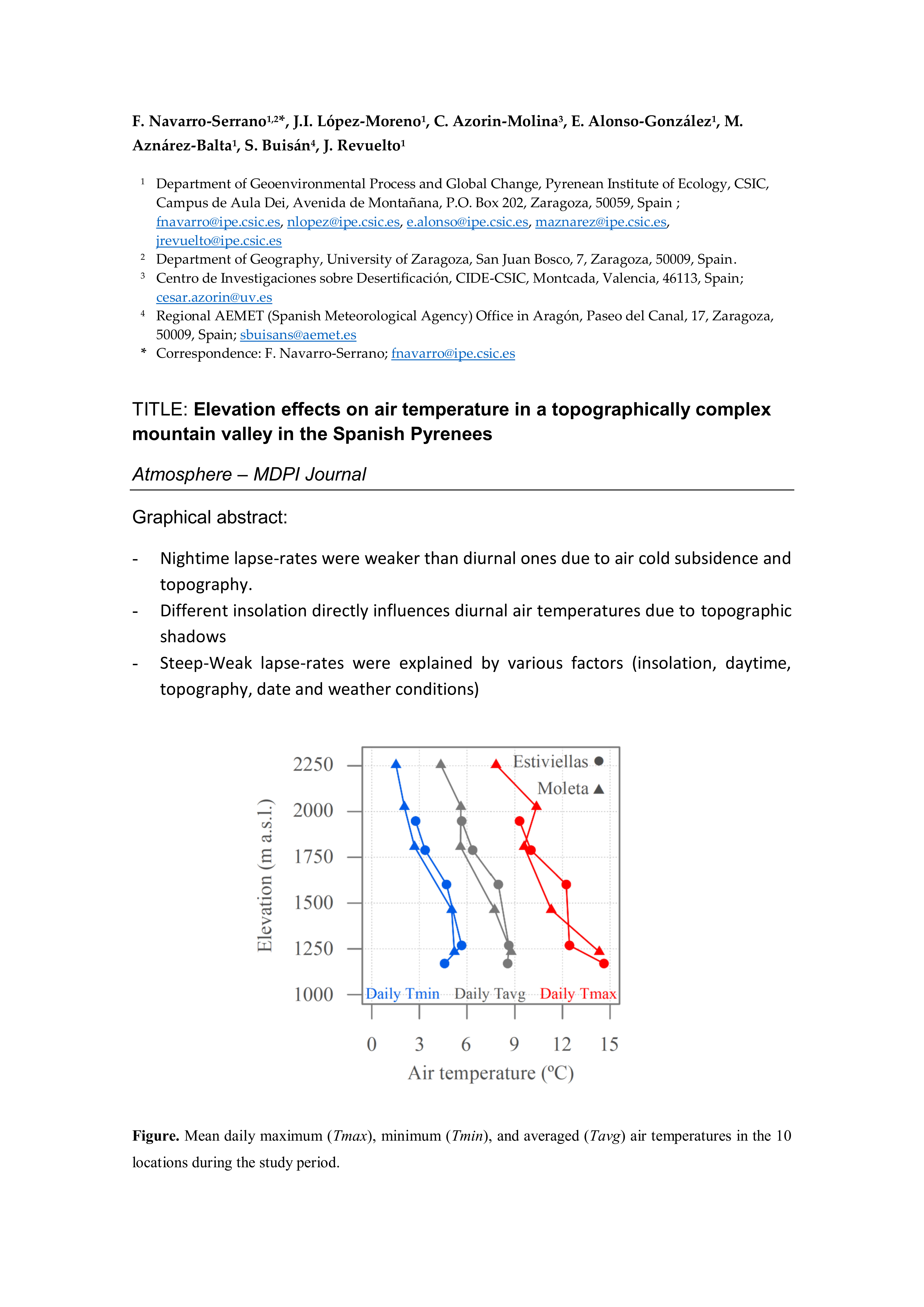
2. Study Area

The Pyrenees are a mountain range in southwestern Europe, separating the Iberian peninsula from the rest of the continent (Figure 1a). Its longitudinal distribution along more than 400 km from west to east causes large differences between the northern French and southern Spanish basins [59], and between the maritime western and Mediterranean eastern side. The highest summits are situated in the axial central Pyrenees (Aneto, 3404 m ASL) with large areas lying over 2000 m ASL, leading to a persistent annual snowpack [57,60]. The Pyrenees host the headwaters of the main tributaries of the Ebro River, contributing to more than 60% of the Ebro River’s total runoff [61]. The Ebro River basin covers areas of scant annual precipitation [62,63], so the water resources generated in the Pyrenees are essential for the entire Ebro basin [64,65].

The Aragón River valley, a tributary of the Ebro River, is located in the headwater zone of the river with the same name, in the western Spanish Pyrenees (Figure 1b). In this region, the climate lies in a transitional area from Mediterranean to Atlantic influence, with abundant rainfall (1500–2000 mm average annual precipitation) throughout the year [66]. The snow season begins at the end of autumn (October–November) and can last until late spring (May–June), disappearing from the summits at the end of summer (August). The most common weather types in absolute terms are anticyclonic, although during winter and autumn the general circulation patterns are more unstable with common frontal passages from the north-west, west and north, usually causing snowfall in cold seasons [67], as well as from the south-west. These atmospheric conditions give rise to significant ski-tourism and hydroelectric generation industries across the region. Moreover, an irregular forest canopy (adjusting to the steep topography and avalanche zones) covers most of the slopes up to 1800 m ASL, with a dominance of evergreen Pinus species with interspersed with diverse deciduous species in the most humid areas [68,69]. Above this treeline, the forest gradually opens and gives way to subalpine meadows and periglacial environments in the summits. Urban areas are very scarce with just a few small villages located at the valley bottom.

The study area is a sector of the Aragon River valley located in the vicinity of the Canfranc-Station village (1100 m a.s.l., 42.75° N, 0.52° W). In this area, the altimetric range covers from 1100 m a.s.l. (river level) to 2573 m a.s.l. (Moleta Peak) in a 2 km transect. This valley section is enclosed to the north (upstream), the east (2500 m mountains) and the west (2350 m mountains), while towards the south (downstream) it is not entirely enclosed, although the river passes through a narrow canyon. The topography is favorable for the generation of cold air pools, although the valley bottom is narrow, so they would not be very extensive. The river crosses the study area from north to south, generating two slopes at opposite sides. The two selected slopes rise to the summit of the Estiviellas and Moleta peaks, facing to the SSE (sunny) and NNW (shady), respectively (Figure 1c).

3. Data and Methods

3.1. Experimental Designs

Ten locations were monitored in this work, 9 of which were installed for this study (

Table 1. Main characteristics of the monitored locations. Elevation is expressed in meters above sea level (m a.s.l.). Latitude and Longitude are expressed in geographical degrees.

Slope	Name	Installation	Elev. m a.s.l.	Land Use	Facing Slope	Lat (°)	Lon (°)
Estiviellas (Sunny)	Est-5	TGP4017 and Datamate	1948	Open Forest	S	42.758	−0.529
	Est-4	TGP4017 and Datamate	1789	Dense Forest	S	42.756	−0.529
	Est-3	TGP4017 and Datamate	1602	Open Forest	SE	42.755	−0.526
	Est-2	TGP4017 and Datamate	1269	Dense Forest	SE	42.756	−0.520
	Est-1	Th. PT100 and Stevenson Sc.	1170	Village	SE	42.749	−0.516
Moleta (Shady)	Mol-5	TGP4017 and Datamate	2255	Open Forest	W	42.738	−0.494
	Mol-4	TGP4017 and Datamate	2026	Open Forest	NW	42.736	−0.502
	Mol-3	TGP4017 and Datamate	1808	Dense Forest	W	42.738	−0.504
	Mol-2	TGP4017 and Datamate	1464	Dense Forest	N	42.740	−0.510
	Mol-1	TGP4017 and Datamate	1234	Dense Forest	N	42.743	−0.515

). The tenth was the Spanish Meteorological Agency (AEMET) weather station (id. 9198X), located in Canfranc-Station village (Figure 1c). Nine autonomous, self-recording and waterproof Tinytag temperature data loggers (http://gemini2.assets.d3r.com/pdfs/original/3239-tgp-4017.pdf) were installed within Datamate radiation shields. The widely used Tinytag dataloggers have a precision error of <0.5 °C, and a resolution of 0.01 °C, while the deviation of the Datamate radiation shield never exceeds 0.5 °C under high solar radiation conditions when compared to the operative AEMET Stevenson radiation screen [36]. The air temperature sensor used in Canfranc-Station corresponds to a Thies PT100 model located in a naturally ventilated medium-sized wooden Stevenson screen [70]. The correspondence and validity of the Tinytag and Thies PT100 sensors and the radiation protection have been previously tested [71,72], and also checked in Canfranc-Station weather station [36], with satisfactory results.

Tinytag dataloggers were placed within radiation shields and hung from tree branches (Figure S1) at a height of ≈2.5 m above the bare ground, which is enough to avoid winter snowpack, according to Navarro-Serrano et al. [36], and >50 cm distant from the main trunk. The evergreen character of the forest ensures an equal canopy cover all year around. To prevent the dataloggers from being affected by excess moisture or condensation, silica bags were placed inside them, and batteries were replaced yearly. Furthermore, our experiment consisted of measuring air temperatures on two opposite slopes (i.e., Estiviellas and Moleta, Figure 1c) to verify the differences between sunny and shady conditions, following the procedures described by Pepin and Kidd [73]. The locations on Estiviellas faced southeast (Est-1, 2 and 3 loggers) and south (Est-4 and 5), while those on Moleta faced north (Mol-1 and 2), west (Mol-3 and 5) and northwest (Mol-4), derived from a 5 m digital elevation model. Thus, the dataloggers were placed at different elevations, from the valley bottom to the highest areas. The aim of the experimental design was to cover, in a homogeneous way, the two slopes, with regular elevational intervals between locations. However, due to the limited number of trees above the timber-line, the dataloggers were placed in scattered trees. This situation, together with the rugged topography, the necessity to follow the only path existing in both slopes, and the need to select suitable trees to ensure an optimal location of the sensors, prevented a fully symmetric placement of elevations between the two slopes. Data were collected by an instantaneous hourly value at LT (local time = UTC + 2 h, Central European Summer Time) during the period between 11 September 2016 and 22 June 2019, generating 24,357 samples for each data series.

Relative humidity and 10-m wind speed data were measured at Canfranc-Station (Figure 1c) by Thies Clima operative instruments, and the atmospheric pressure in the weather station of Aragués del Puerto (AEMET “9208E”, located at 10 km, Figure 1b) by the operative instrument Vaisala PMT, at 10-min measuring intervals. In addition, to better evaluate the results, land cover was classified into the different land covers presented in the study area cartography.

3.2. Climate Data and Quality Control Checks

Air temperature data were checked by applying a quality control that ensured that the dataloggers were not buried under snow. For this, daily air temperature ranges were analyzed, discarding those days with hourly standard deviation < 0.1 °C and an average air temperature < 2 °C. The air temperature in snow-burial conditions was constant at a value close to 0 °C [74], so it was relatively easy to filter out this issue. The 10 locations passed this filter and 0 samples were discarded. However, the raw experimental design had 11 locations, of which one (Est-6, at 2067 m a.s.l.) had to be removed in this quality control check. This location suffered problems from December to May, affecting 5422 hourly samples (22.3% of the study period). Furthermore, a total amount of 60 hourly samples (0.02% of the total) were discarded due to annual battery changes. Of these, 23 were gaps of less than two continuous samples, so they were filled by a regression model based on the best neighboring air temperature series for that month. The remaining data were maintained as Not Available (NA) data.

Next, the hourly samples were summarized by day using the air maximum (Tmax), minimum (Tmin) and average (Tavg) temperature of the raw 24-hourly samples for each location. It was verified that more than 90% of hourly samples were available each day. Raw weather data measured at Canfranc-Station and Aragués del Puerto were summarized according to the daily mean atmospheric air pressure (in hPa), the daily mean relative humidity (in %) and the daily mean 10-min wind speed (in m s⁻¹).

3.3. Lapse Rate Calculation

Air temperature LRs were calculated for both the Estiviellas and Moleta slopes at hourly time steps (LR_h), and for daily maximum (LRmax), minimum (LRmin) and average (LRavg) air temperatures. Following procedures outlined by Rolland [75], Du et al. [76] and Navarro-Serrano et al. [41], regressions were used to determinate LRs, formulated in Equation (1) as:

T′ = a₁ Elev + e,

(1)

where T′ is the estimated air temperature (in °C), Elev is the elevation above sea level (m a.s.l.), e is the regression error and a₁ is the regression coefficient, which corresponds to the air temperature elevational LR. Latitude and longitude variables can be included in the model, but the effect in such a small study area is usually negligible due to the short distances between locations. The regression model approach has been used by other authors [42,44,77], and provides an appropriate way to analyze the effects of elevation on air temperature distribution. The influence of synoptic conditions can be analyzed subsequently. All these LRs were also calculated among all the combinations for the locations. To clarify the interpretation of the LR values, when in the following paragraphs we refer to a “steeper” LR and a “weaker” LR, we refer to a larger change in air temperature with elevation, and a smaller change, respectively (e.g., −7.2 °C km⁻¹ is steeper than −4.3 °C km⁻¹).

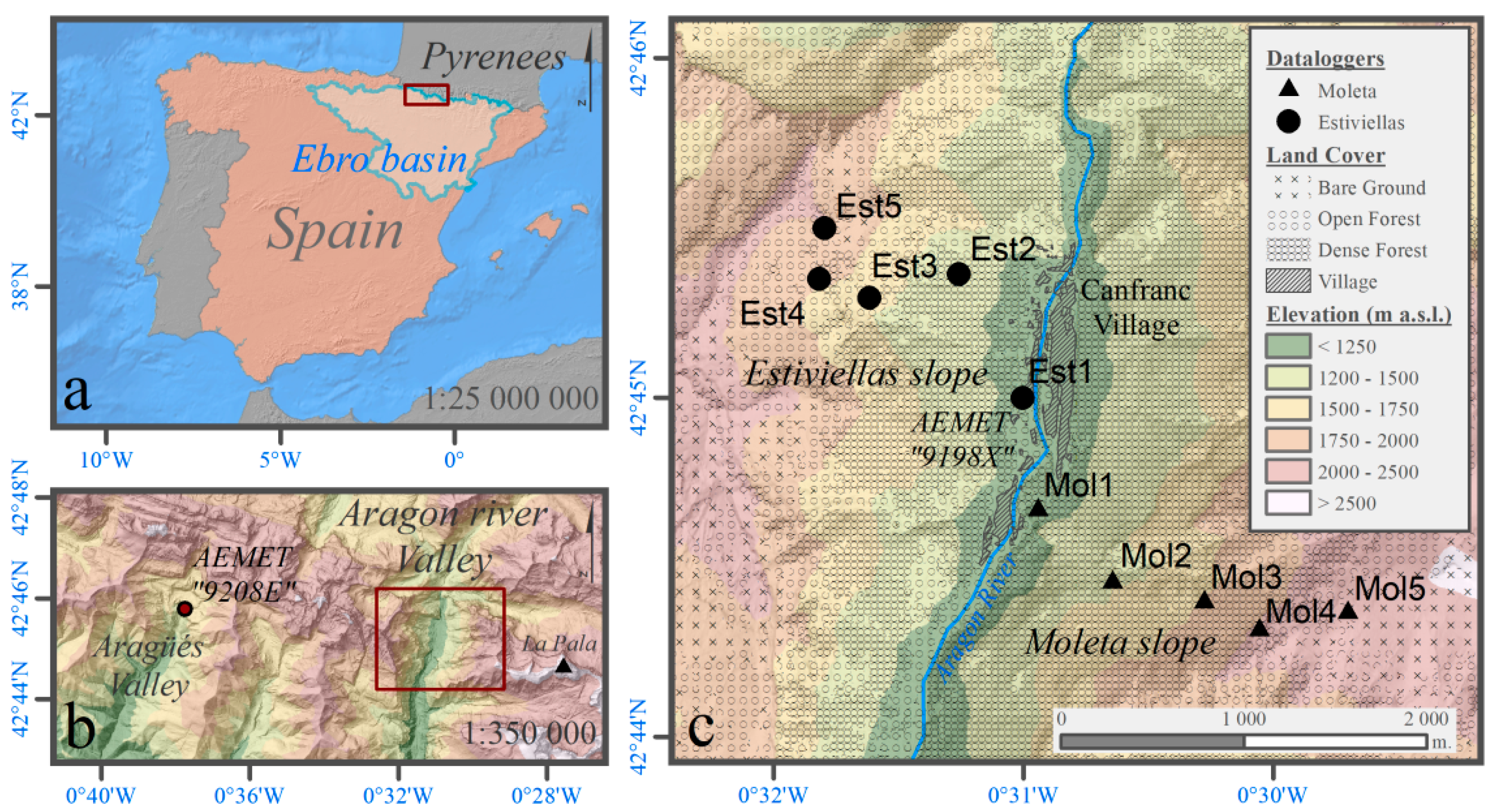
3.4. Estimated Solar Radiation

The amount of solar radiation received by the terrain [16,45], topographic shadows and surface orientation are crucial to better understand the spatiotemporal distribution of air temperature, especially during daylight hours [78]. To obtain this information, we used a digital elevation model (DEM5) with 5 m spatial resolution purchased from the PNOA-LiDAR program [79]. The instantaneous solar radiation estimation under clear sky conditions by hour was estimated by applying the insolation function of the R package “insol” [80], developed for R language version 3.5.0 [81]. This function takes into account diffuse radiation, in addition to air temperature, humidity, date and location, to estimate instantaneous insolation (in W m⁻² s⁻¹). The solar radiation estimated in each monitored location throughout the year and summarized by seasonal (i.e., winter: December–February; spring: March–May; summer: June–August; autumn: September–November) hourly means (Figure 2) shows variability due to topographic conditions and differences between the Estiviellas and Moleta slopes (sunny and shady, respectively). In addition, this dataset clearly displays the topographic shadows occurring in the bottom location of the study area, mainly on the Moleta slope, and during winter. This estimated information allows the identification of the characteristics of the monitored locations, which allow discussion of the results keeping in mind the effect of topography on solar radiation reception.

3.5. Circulation Weather Types Classification

Circulation weather types (CWTs) at daily scale over the Pyrenees were calculated using Jenkinson and Collison’s [82] classification method, based on Lamb’s weather types [83] and simplified satisfactorily by Rasilla Álvarez et al. [84] and Navarro-Serrano et al. [41] for the Iberian peninsula. This version classifies the raw CWTs into two pure (anticyclonic-A and cyclonic-C), eight directional (north-N, northeast-NE, east-E, southeast-SE, south-S, southwest-SW, west-W and northwest-NW) and one unclassifiable (U) CWT, prioritizing directional flows in hybrids. The method is based on the distribution of sea-level atmospheric pressure in a 16-point grid covering an area of 30 × 20° (longitude × latitude) centered on the study area. This information was obtained from the NCEP-NCAR reanalysis (5 × 5° longitude-latitude) dataset [85]. To simplify the analysis, U days were not represented, but were computed in the total amount of days. The frequency of CWTs is shown in Figure S2.

3.6. Cluster Analysis

To analyze different patterns in the daily elevational distribution of maximum (Tmax), minimum (Tmin) and average (Tavg) air temperature, a cluster analysis was applied. Cluster analysis is a multivariate statistical technique, that is, it analyzes the behavior of three or more variables simultaneously, aiming for the creation of clusters or groups that have large internal homogeneity and maximum difference in relation to the other groups. This process is carried out automatically, based on the study of daily temperatures in relation to highest location of each slope and the creation of clusters based on the distances between them. Daily air temperature differences between the Tmax, Tmin and Tavg of each location and the reference datalogger of its slope (i.e., the highest: the Est-5 [1948 m] and Mol-5 [2255 m] loggers on the Estiviellas and Moleta slopes, respectively) were computed. These new series were employed as input variables for the cluster analysis, which, in function of the air temperature difference of each location in relation to the highest one, generated groups or clusters of days with similar behavior. In this way, similar (close) days were classified in the same cluster, while distant days were classified in different clusters.

The number of clusters was determined by executing the NbClust function of the R package “NbClust” [86], which analyzes 30 different indices to determine the most appropriate number of groups using Euclidean distance and the hierarchical Ward.D2 method [87], minimizing the total within-cluster variance. After determining the appropriate number for each combination (Tmax/Tmin/Tavg and the Estiviellas and Moleta slopes), a cluster analysis was run using the Ward.D2 and Euclidean distance parameters. This classified each day according to the nearest cluster centroid. Differences between pairs of clusters were compared by the Wilcoxon–Mann–Whitney test [88] to identify statistically significant differences among groups. In cases of 3 clusters, these were compared between pairs (i.e., 1 and 2, 1 and 3, 2 and 3). This nonparametric statistical test allows the similarities/differences between two independent samples to be tested. Differences were tested at a 0.05 significance level.

4. Results

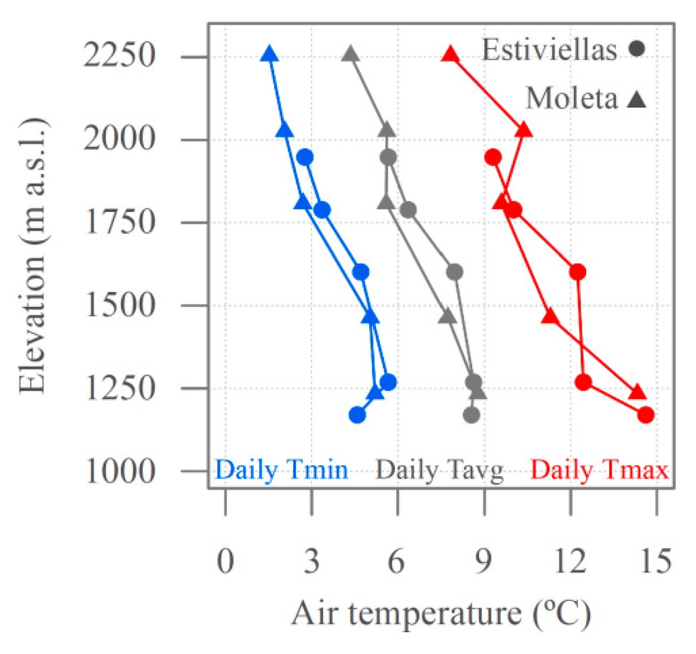
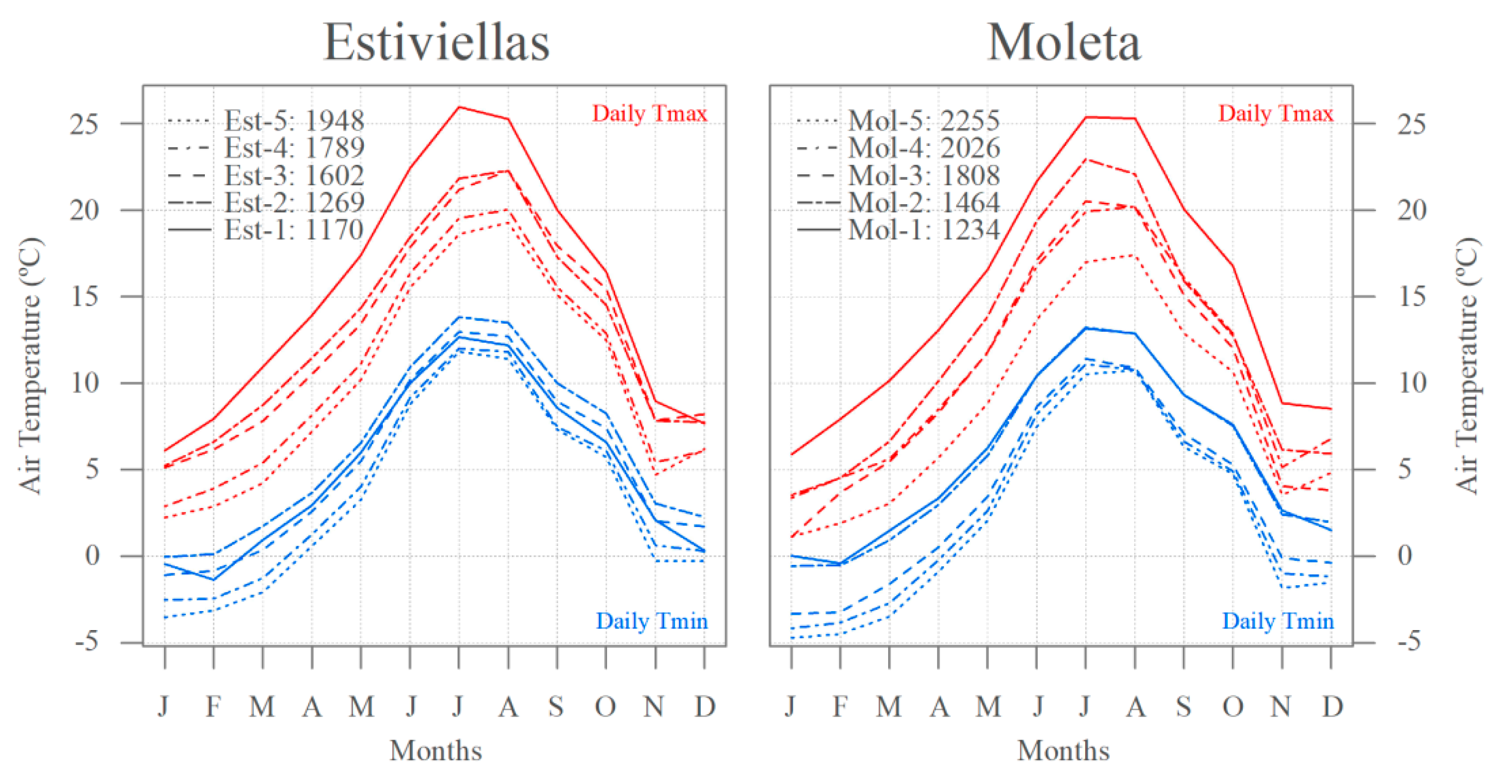
4.1. Air Temperature

The daily mean maximum (Tmax), minimum (Tmin) and average (Tavg) air temperatures for each of the ten locations are shown in Figure 3. Although an inverse relationship between air temperature and elevation exits, this is not linear. Moreover, there were differences between the behaviors of Tmax/Tmin/Tavg, and between the two opposing slopes. The air temperature across the study area varied from a mean Tmax around 15 °C at the valley bottom to 10 °C at 2000 m a.s.l. Tmax differences are noticeable between the slopes, showing a decoupling between the two faces at mid-slope locations, mainly due to the variable behavior of Est-1 and Est-2 and heating at the Mol-4 location. Tmin shows a more complex relationship with elevation, especially at the valley bottom. Above the slopes, Tmin was around 5 °C at 1500 m ASL and 2 °C at 2000 m a.s.l. Unlike Tmax, Tmin shows similar patterns between both the Estiviellas and Moleta slopes, except for at Est-1, i.e., the location at the valley bottom.

The monthly air temperature patterns for Tmax and Tmin among the ten locations are shown in Figure 4. The Estiviellas slope presented the expected inverse relationship between elevation and Tmax for most of the year, although it presented some nuances during August and December between the Est-2 and Est-3 locations, which had similar Tmax values. However, the Moleta slope returned an irregular elevation–Tmax relationship throughout the year (except from June to August). Tmax differences between the lower and higher locations increased during June and July, decreasing from September to November. Furthermore, the elevation–Tmin relationship was less evident. The Estiviellas location with the warmest Tmin throughout the year was Est-2, while Est-1 and Est-3 had similar values, but were cooler than Est-2. On Moleta, a decoupling between its three highest and its two lowest locations was found (probably as a result of the larger elevational distance between them). For instance, Mol-1 and Mol-2 had similar Tmin values throughout the year, with Mol-1 being slightly colder than Mol-2 in December. Mol-3, Mol-4 and Mol-5 kept their positions, but presented similar air temperature values from July to September.

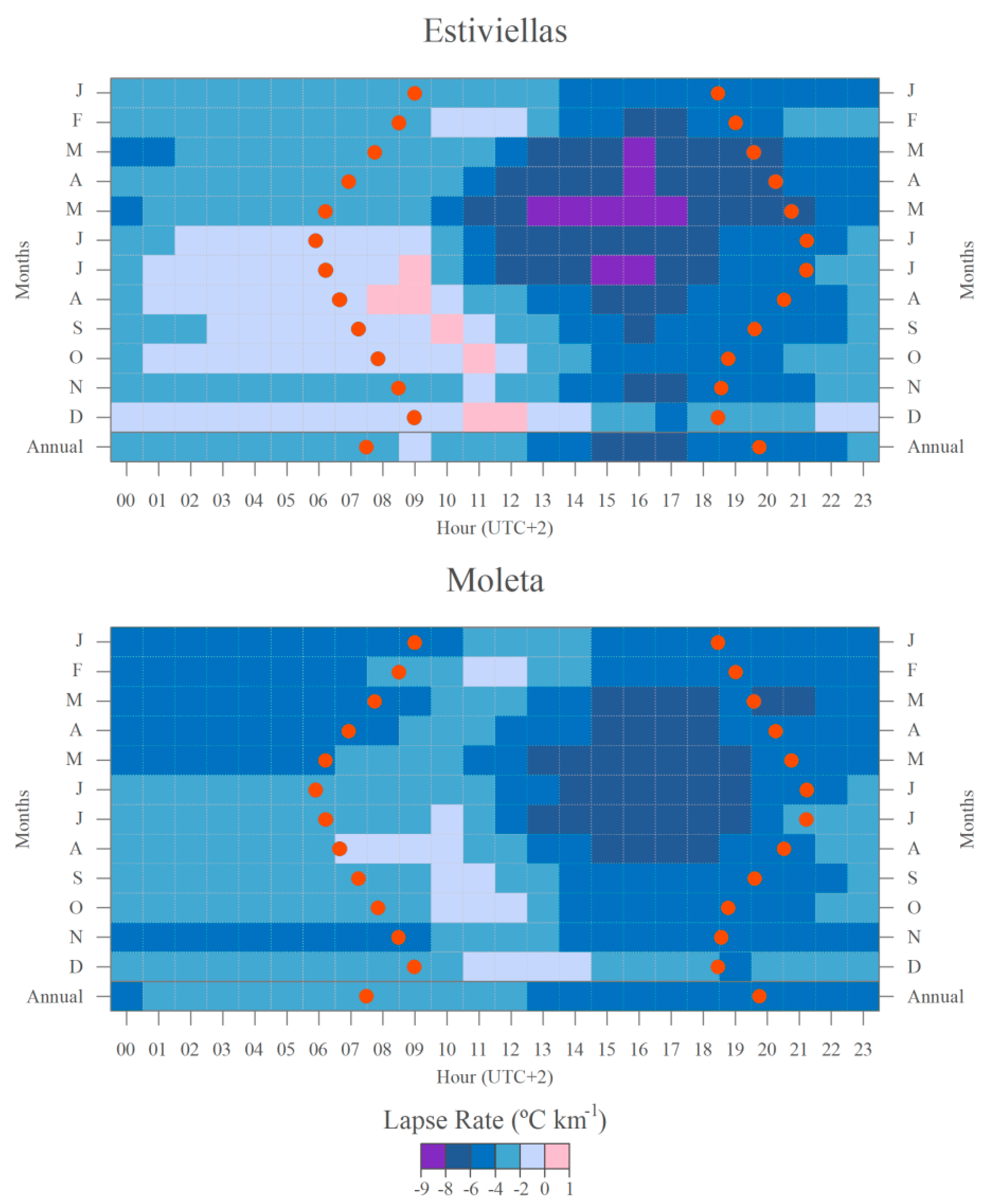
4.2. Hourly Air Temperature Lapse Rates (LR_h)

In Figure 5, both the Estiviellas and Moleta slopes show weak LR_h (local time UTC + 2) during the night (especially at sunrise, calculated by the methodology explained in Section 3.4), and high LR_h in the afternoon. This pattern occurred every month, although with a time shift caused by the expansion of weak LR_h during the winter months, and narrowing during the spring and summer months. In absolute terms, LR_h was around −4 and −2 °C km⁻¹ at night and sunrise (even weaker on Estiviellas at 9 h UTC + 2), and around −6 and −4 °C km⁻¹ in the afternoon (even steeper on the Estiviellas slope from 15 to 17 h UTC + 2). These hours showed a slight seasonal shift, with weaker LR_h delayed during the winter months, and occurring earlier during the spring and summer (e.g., the weaker LR_h in Estiviellas occurred at 9 h UTC + 2 during August and at noon during December), so the LR_h was steeper in June than in December.

Both the Estiviellas and Moleta slopes had a similar seasonal pattern at the hourly resolution, since steepness of LR_h occurred from May to July in mid-afternoon, while the weakest LR_h occurred in December at night. LR_h was weaker during the night from June to October than from January to May, and steeper during the afternoon from March to August than from September to February. However, we found significant (p < 0.05) differences in the slope of the LRs between the two slopes, since in Estiviellas they ranged from −8.90 (May at 16 h UTC + 2) to +0.80 °C km⁻¹ (December at 12 h UTC + 2), and in Moleta from −7.46 (July at 17 h UTC + 2) to −1.01 °C km⁻¹ (August at 10 h UTC + 2). The coefficients of variation were calculated and shown in Figure S3. This figure shows that the most favorable hours for thermal inversion were those that generated the largest variability (early morning and night).

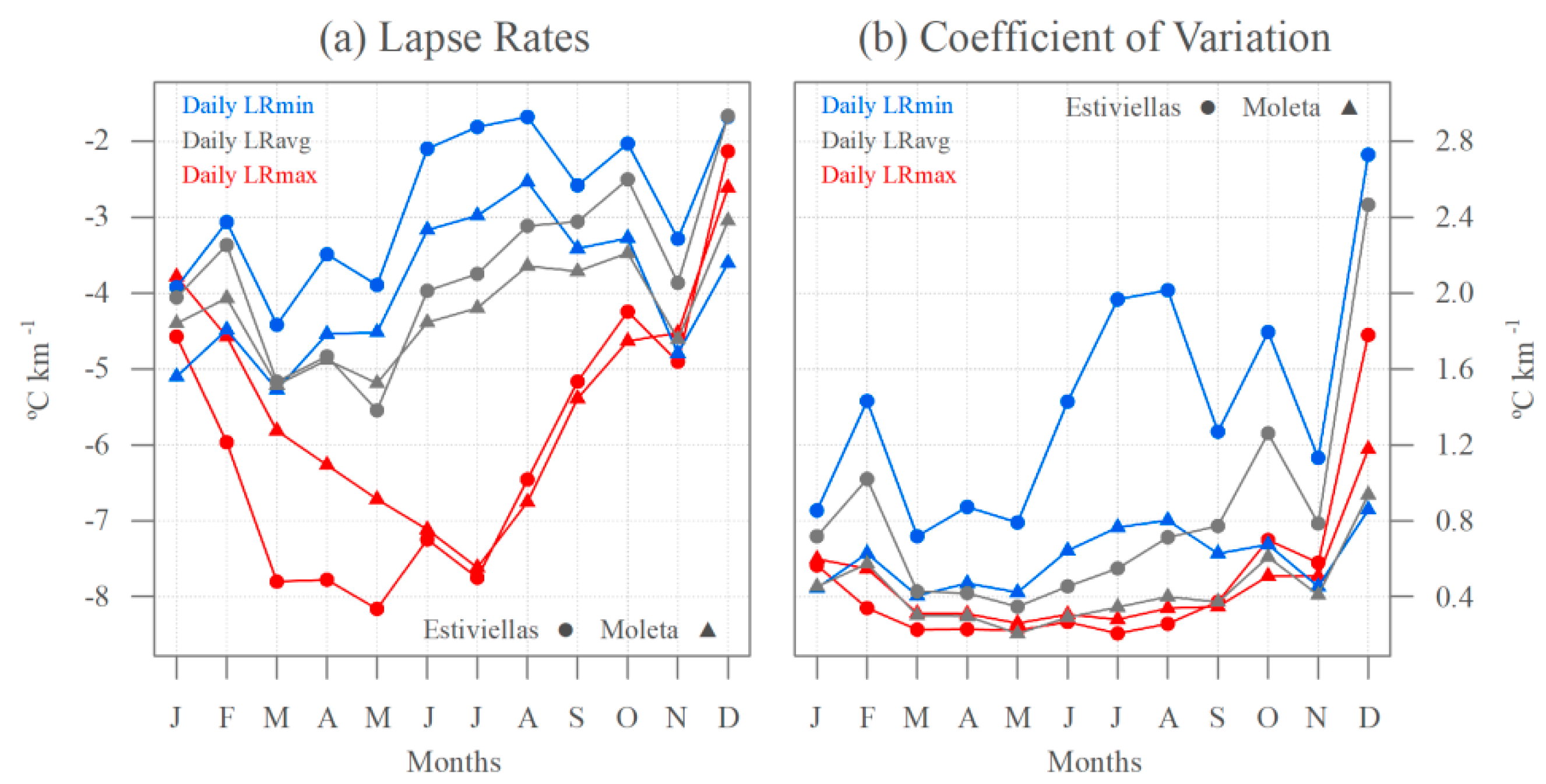
4.3. Monthly Maximum (LRmax), Minimum (LRmin) and Average (LRavg) Air Temperature Lapse Rates

Figure 6a shows that, generally, LRmax was steeper than LRmin on both the Estiviellas and Moleta slopes (p < 0.05). LRavg returned mixed behavior between LRmax and LRmin. The annual data support this fact, through an annual average LRmax, in °C km⁻¹, of −6.0 (−5.5), and a LRmin annual average of −2.8 (−4.0) for the Estiviellas (Moleta) slope. This pattern was present during most of the year, although it intensified during the summer (e.g., July). The differences in winter were smaller and even reversed from November to January on the Moleta slope. LRmax weakened from October to February and became steeper from March to July. LRmin was also steeper from March to May, but weakened from June to August (and December). In any case, although there were seasonal differences, LRmin showed low variation in absolute terms (−4.4 to −1.7 on Estiviellas; −5.3 to −2.5 on Moleta) compared to LRmax (−8.1 to −2.1 on Estiviellas; −7.6 to −2.6 on Moleta). LRavg returned mixed behavior between LRmax and LRmin, but was much closer to LRmin. The comparison between the two slopes showed that the LRmax was similar from June to December, with a steepening on Estiviellas from January to May. LRmin was similar between both slopes throughout the year, although steeper on Moleta.

Figure 6b shows monthly variability based on LRs by the coefficient of variation. In general terms, LRmin had larger variability than LRmax, especially on Estiviellas. Seasonally, the LRmin coefficients increased during the summer (e.g., June to August) and December. On the contrary, in spring (March–May) and autumn (September–November) the coefficients were the lowest of the year. LRmax had reduced coefficients throughout the year (generally <0.8 °C km⁻¹), which increased gradually during autumn, with the highest value in December (>1 °C km⁻¹). The LRmax, LRmin, and LRavg calculated between partial sections on each slope are not shown, but their behavior was extremely variable and wide-ranging, demanding the use of all available datalogger series to calculate the LRs on each slope.

4.4. Cluster Analysis

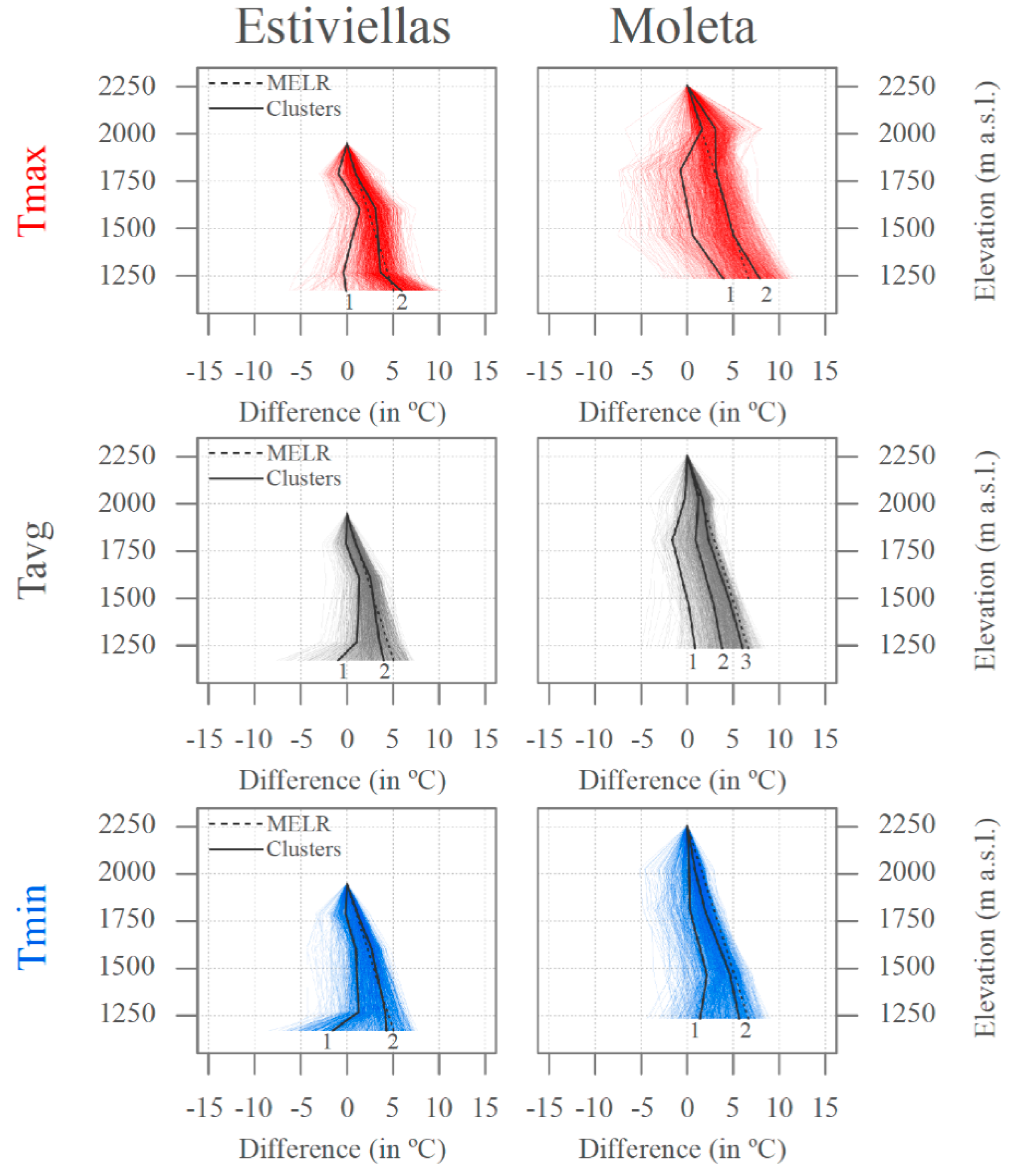
4.4.1. Cluster Classification

Figure 7 shows the air temperature differences from each monitored location to the highest measured level on each slope (i.e., 1948 m a.s.l. in Estiviellas, and 2255 m a.s.l. in Moleta), with a noticeable daily variability in air temperature profiles. The figure shows a dynamic and continuous relationship between air temperature and elevation, where it is difficult to visually establish linear patterns along the entire slopes. However, cluster analysis allows daily profile types to be established with a statistical approach. For maximum air temperatures, bottom locations were usually warmer, but the profiles throughout the entire slope were not completely linear. For minimum air temperatures, the lowest Estiviellas location (1170 m a.s.l.) had an inverse relationship with the rest of the slope, less evident on Moleta. In this way, cluster analysis generated the optimal number of profile typologies, with the mean values given in

Table 2. Tmax, Tmin, and Tavg cluster centroid values for the Estiviellas and Moleta slopes. Loc = location order, from bottom (1st) to top (5th).

	Estiviellas			Moleta
Tmax	Loc.	Cluster 1	Cluster 2	Loc.	Cluster 1		Cluster 2
	5th	0	0	5th	0		0
	4th	−0.92	+0.94	4th	+1.62		+3.04
	3rd	+1.41	+3.15	3rd	−0.73		+3.11
	2nd	−0.38	+3.62	2nd	+0.60		+5.02
	1st	−0.09	+5.96	1st	+3.93		+7.89
Tavg	Loc.	Cluster 1	Cluster 2	Loc.	Cluster 1	Cluster 2		Cluster 3
	5th	0	0	5th	0	0		0
	4th	−0.10	+0.94	4th	−0.25	+1.24		+1.64
	3rd	+1.37	+2.58	3rd	−1.61	+0.91		+2.32
	2nd	+1.08	+3.53	2nd	+0.14	+2.87		+4.74
	1st	−0.96	+4.00	1st	+0.87	+3.78		+6.01
Tmin	Loc.	Cluster 1	Cluster 2	Loc.	Cluster 1		Cluster 2
	5th	0	0	5th	0		0
	4th	−0.14	+1.16	4th	+1.38		+0.82
	3rd	+0.97	+2.69	3rd	+2.14		+1.92
	2nd	+1.25	+4.15	2nd	+0.30		+4.67
	1st	−1.57	+4.31	1st	+0.18		+5.62

. Other than the air average temperatures on Moleta (three clusters), the remaining combinations each generated two clusters. The clusters were ordered from weak to steep lapse rates (i.e., Cluster 1 represents the group of weakest lapse rates).

Clusters generated from maximum air temperatures were similar in form, but differences arose from the degree of difference to the reference highest locations. The LRmax values for Cluster 2 from Estiviellas and Moleta were close to the MELR, with much warmer bottom location values. The contrasting behavior between Cluster 1 and Cluster 2 was more clearly present in air minimum temperatures, where LRmin values for Cluster 1 from Estiviellas and Moleta were decoupled from those for Cluster 2, especially in the bottom locations. In the average air temperatures, a more linear behavior can be observed along the slopes, especially on Moleta, where three clusters were generated. However, Cluster 1 from Estiviellas was inverted in its bottom location.

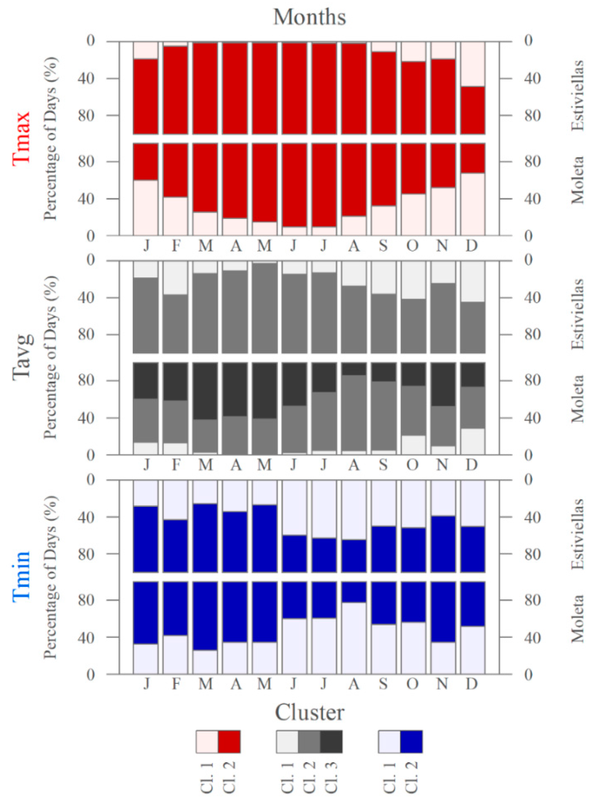
4.4.2. Monthly Distribution of Clusters

Figure 8 shows the monthly distribution (% of days) of each cluster throughout the year. On the one hand, the cluster associated with steep LRmax (Cluster 2) was more common than the weak LRmax cluster (Cluster 1), especially from March to August (>80% of “steep” days). On the other hand, the days classified with weak LRs increased in frequency from September to January, becoming as frequent as those with steep LRs, especially along the Moleta slope (≈50%). LRmin cluster frequency was more equal on the two slopes. However, Cluster 2, associated with steep LRmin, was more common from January to May (>50% of days), and Cluster 1 from July to December. On Estiviellas, the frequency of LRavg Cluster 1 was higher during the summer and December and lower/null in spring. On Moleta, despite having three LRavg clusters, the same pattern was repeated, although less frequently for Cluster 1. On Moleta, in any case, LRavg was dominated by medium and steep clusters (Clusters 2 and 3, in most months generally >80%) over the weak Cluster 1, although the latter increased in frequency from August to February.

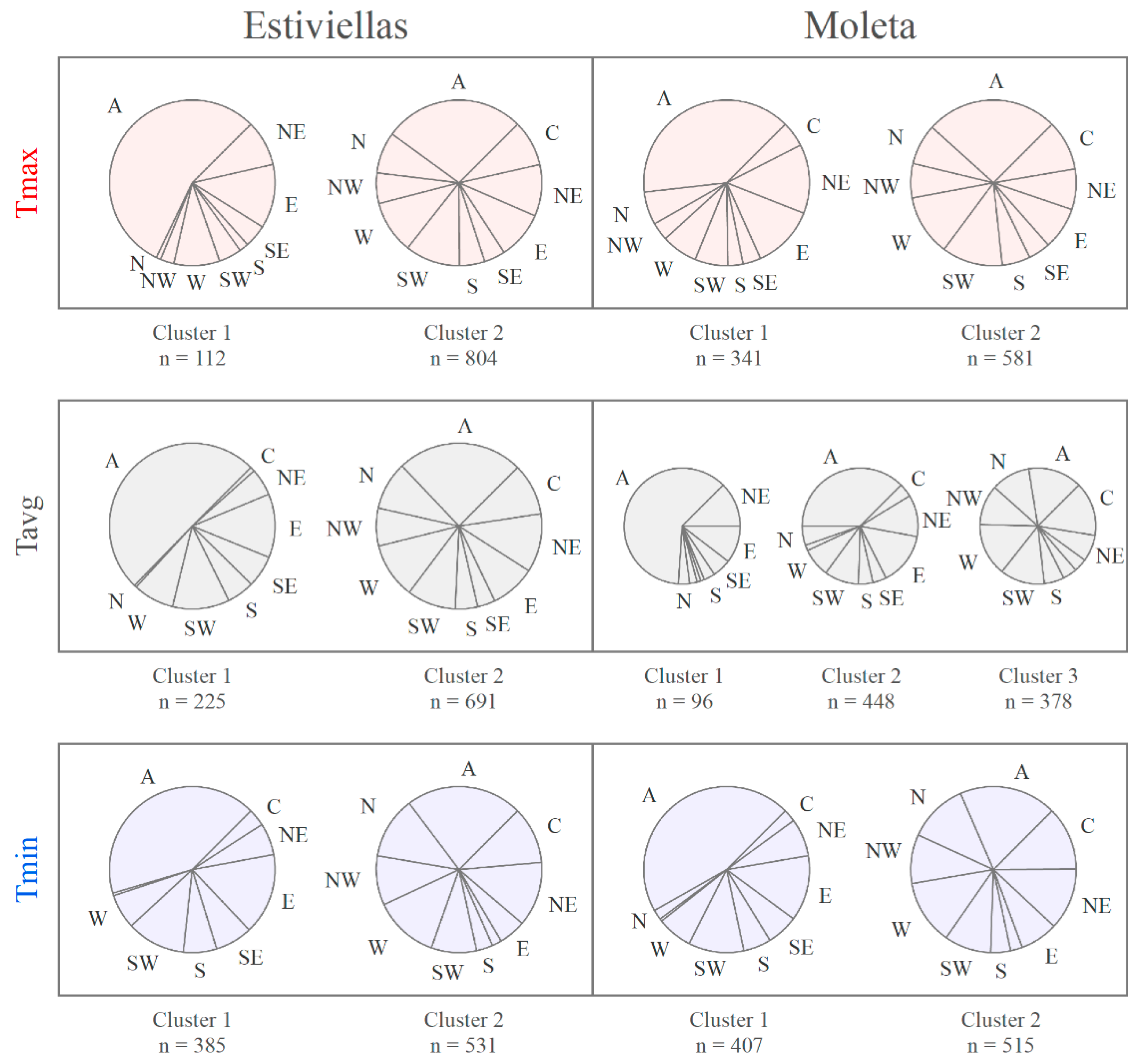
4.4.3. Clusters, Circulation Weather Types and Weather Conditions

To analyze the synoptic and weather patterns found during each cluster day, Figure 9 shows the circulation weather type (CWT) distribution. Atmospheric pressure (Figure S4), relative humidity (Figure S5) and wind speed (Figure S6) variability for each cluster are also presented.

Days classified within the Tmax Cluster 1 (associated with weak LRmax) were dominated by anticyclonic (A) and NE and E circulations (Figure 9), accompanied by higher atmospheric pressures (≈1026 hPa) and lower relative humidity (≈69.4%), although no clear wind speed pattern was found on those days. On the contrary, when analyzing the Tmax Cluster 2 (associated with steep LRmax) no particular CWTs prevailed, except for some westerly and northerly circulations, and also the anticyclonic-A and cyclonic-C types. However, atmospheric pressure values were lower (≈1.019 hPa), relative humidity values were higher (≈75.1%) and wind speed was variable. Wind speed daily values between Tmax clusters in Estiviellas were compared and were significantly different (p < 0.05). The same occurred when comparing the values of atmospheric pressure and relative humidity (also on the Moleta slope). Thus, days associated with each cluster differed not only in the behavior of the air temperature, but also in other meteorological variables measured.

For Tmin, days classified within Cluster 1 (associated with weak LRmin) were marked by a clear dominance of the A weather type, weaker winds (≈2.1 m s⁻¹, especially on Estiviellas), higher atmospheric pressure (≈1023 hPa) and lower relative humidity (≈70.9%). Tmin Cluster 2 (associated with steep LRmin) was represented by different circulation types (e.g., northerly, westerly and C, among others), moderate to strong winds (≈3.9 m s⁻¹), lower atmospheric pressure (≈1019 hPa) and higher relative humidity (≈76.2%). The same pattern occurred for Tavg values, although the three Tavg clusters on Moleta showed the anticyclonic dominance of weak lapse rates more clearly. As with Tmax clusters, the differences between Tmin clusters were statistically significant (p < 0.05) for wind, relative humidity and atmospheric pressure, again on both slopes. The air temperatures from bottom-summit locations during the extreme period from 3 December 2017 and 5 December 2017 are presented in Figure S7 to show the transition between unstable and stable weather types, together with atmospheric pressure and wind speed. The moment at which wind speed fell coincided with the beginning of thermal inversion between Est-1 and Est-2 (and almost between Mol-1 and Mol-5). Similarly, the lowest atmospheric pressure values coincided with the largest differences between the locations, and vice versa.

5. Discussion

The air temperature and lapse rates in two opposite steep and complex slopes (i.e., sunny Estiviellas and shady Moleta) of the upper Aragon river valley (Spanish Pyrenees) were analyzed in ten locations (elevations ranging from 1170 to 2255 m a.s.l.) for 1015 consecutive days from September 2016 to June 2019. Following previous studies, such as Barry [16] and Lookingbill and Urban [45] for North America, this one analyzed the relationship between air temperature and local terrain characteristics (e.g., facing slope, insolation, land cover, weather types and atmospheric parameters such as air pressure, relative humidity and wind speed). This study focused on a single Pyrenean valley, complementing previous regional work on the Iberian peninsula [41,89,90]. Also, the study of diurnal lapse rates at this local scale provided new information for this region of Europe, which has mainly been investigated for its night-time cold air pools [33,34,73].

The results show variable insolation values within and between slopes, as in Lookingbill and Urban [45]. The differential insolation has a direct effect on air temperature distribution and variability [31,91,92]. The lesser insolation at the valley bottom, more significant in the lower locations on the shady Moleta slope, especially around December, was consistent with the complex topography. Direct insolation on the Moleta slope is very limited during the autumn and winter months, as we can see in Figure 1 and Figure 2. On the other hand, in higher locations on Moleta, more insolation was estimated due to the increasing sky view factor, reducing the differences in relation to the sunny Estiviellas slope. At this point, the use of digital elevation models of high spatial resolution is essential to represent the terrain reliably. Other local differences could be explained by land cover, such as the diurnal overheating of the Est-1 (village) location in comparison with Est-2 (dense forest), or the combined effect of the low insolated and dense forested locations (e.g., Mol-3 and Mol-4), according to the buffering effect of the forest canopy [49]. Therefore, the results show that elevation is not a factor with a linear effect, but that there are local variables that can alter the diurnal air temperature distribution [76]. At night, the topography also exerts an effect, as the valley bottom locations demonstrated by capturing thermal inversion phenomena, according to papers on cold air pools [17,23,93]. Partial LRmin between Est-1 and Est-2 were close to +20 °C km⁻¹ of thermal inversion, which agrees with the extreme values registered by Pepin and Kidd [73] and Pagès et al. [33] in the Cerdanya valley in the eastern Pyrenees. More variance was detected in Tmax than Tmin both between and within slopes, showing a strong influence of land cover on Tmax, which caused inversions between the Est2/Est3 and Mol3/Mol4 locations, due to the correspondence with the treeline ecotone. To summarize, air temperatures registered at each location were not only the result of elevation, but also of effects caused by insolation, topography and land cover.

In terms of lapse rates, the hourly analysis in Section 4.2 allowed the continuous identification of the behavior throughout the 24 h sections and the months of the year. In this way, the analysis has a larger wealth than analysis of the daily max and min air temperature moments exclusively, being able to show other nuances between the slopes. Thus, this analysis showed the influence of insolation on thermal mechanisms, with a weakening of the night-time lapse rates due to cold air subsidence from the summits to the valley bottom [77,94,95]. Thus, the weakest hourly lapse rates occurred in the morning (+0.81 °C km⁻¹ in December at 12 h in Estiviellas, and −1.02 °C km⁻¹ in August at 10 h in Moleta, Central European Summer Time time zone). This is because that is the time when insolation reaches the highest locations, while the lower ones remain shady, according to insolation data, and with an accumulation of cold night air. However, insolation is seasonally variable (later in December, and earlier in July). These results are in agreement with Pagès et al. [33]. Moreover, the steepest lapse rates took place in the early afternoon and were explained by high insolation in the lower locations, especially on Estiviellas, which broke up the cold layers and steepened the relationship between elevation and air temperature (on Moleta the lapse rates were less intense). Later, the sun begins to descend and the topographic shadows reach the low locations first, reiterating the process [50].

The results show that LRmin were generally weaker than LRmax (total mean of −2.8 vs. −6.0 °C km⁻¹ on Estiviellas, and −4.0 vs. −5.5 °C km⁻¹ on Moleta), as in most similar studies around the globe [8,94,96], which attribute it to the previously mentioned nocturnal cold air subsidence toward the bottom areas. However, this behavior changed through the year, since the differences were larger in summer (diurnal steepening along the slope in addition to nocturnal weakening), and smaller in winter (diurnal weakening due to topographic shadows in addition to nocturnal weakening). This supports the hypothesis that topographic shadows affect air temperature distribution during the daytime [10,78]. This process was also corroborated by decoupling between the Estiviellas and Moleta LRmax from March to May when the Estiviellas slope was completely insolated. However, on Moleta, the insolation did not yet reach lower locations. This comparison between sunny and shady slopes can only be observed where the topography is abrupt enough to generate permanent topographic shadows that alter air temperatures, and not in open valleys. The existence of snow cover in higher locations has also been mentioned as a reason for the steepening of LRmax [31], due to the albedo effect in elevated areas, in which snow cover persists during the spring months. This could explain the peak delay between the LRmax in Estiviellas (June) and Moleta (July), due to the longer snow season on the northern Moleta slope [97]. It would be very useful to advance the study of this issue in the future, and analyze the importance of this factor.

However, the study of the monthly coefficients of variation has confirmed that the monthly LR values derived from a linear fit are not entirely representative, since they hide different internal behaviors, especially in the LRmin. To deepen the study of LR patterns from a global (and non-linear) perspective, a cluster analysis was performed. In this respect, the cluster analysis showed that, regardless of the month, there were usually two distinct profile patterns (weak vs. steep), and that these could occur at any time of the year, although there were more propitious moments. In general terms, the steep clusters were close to the MELR (−6.5 °C km⁻¹). This method was proposed by Barringer [98] to classify days based on air temperature profiles. The merged analysis between clusters, insolation, circulation weather types and weather conditions supports the hypotheses, since it shows a broadly weak LRmin with stable conditions, high atmospheric pressure, low relative humidity and weak winds, according to the majority of studies on Cold Air Pools [34,40,44,73], and the regional results of Navarro-Serrano et al. [41] in the Pyrenees. On the other hand, steep LRmin occurs under conditions of instability, dynamic weather types, low atmospheric pressure, high relative humidity and strong winds, which explains the breakup of cold layers and the prevalence of the free-air lapse rate [1,27,33,77,99,100].

However, Tmax clusters were more complex than expected prior to beginning this research, unlike claims by other authors on a regional scale [41,101]. This is due to the previously explained complex topographic conditions of the study area, which are more influential during the winter months. The results show that the Tmax clusters associated with steep LRmax were more frequent than those associated with weak ones, especially during spring and summer, according to Minder et al. [28]. As mentioned above, LRmax intensified during the summer due to the insolation reaching the lower locations, and in spring also due to more frequent cloudy days under unstable meteorological conditions. Therefore, these Tmax clusters associated with steep LRmax were accompanied by varied CWTs and wind speed conditions, since they occurred under diverse synoptic situations (e.g., sunny summer days and rainy March days) [34,94]. Furthermore, Tmax clusters associated with weak LRmax only occurred under topographic shadows (i.e., more frequently in winter, anticyclonic situations, high atmospheric pressure and low relative humidity). This is because LRmax returned a high coefficient of variation in winter (e.g., a sunny stable winter day weakens LRmax, and a cloudy one steepens it; and yet in summer, both unstable and stable sunny days steepen LRmax). In any case, the limitations of the use of humidity and wind speed valley bottom measurements should be taken into account. Although we think that it can be representative of the timings of higher or lower humidity/wind speed in the whole valley, we cannot assume that this is absolutely right, and it should be analyzed in the future with more information. To summarize, local terrain factors must be taken into account, especially in study areas with complex terrain [102]. In these cases, the same synoptic conditions could generate different effects on lapse rates, depending on the position of the sun and azimuth. This is an approach that has been recognized in some studies on persistent cold air pools [50,103].

Therefore, although previous work has tried to analyze the variability of LRs based solely on synoptic conditions, this analysis reveals that insolation, heavily affected by topographic shadows, has noticeable impact on diurnal air temperature variability. Thus, terrain factors such as sky view factor, aspect, forest canopy must be taken into account when designing experimental measurement networks in mountain terrain, so that these factors are not underestimated when analyzing LRmax. LRmin analysis has corroborated findings from previous studies on the influence of synoptic conditions and topography [104]. Future research should carry out in-depth analysis of the variability of the air temperature along a slope. Factors such as weather conditions, insolation, aspect, and topography have been shown to be explanatory variables for air temperature distribution in topographically complex areas, although they have often been underestimated in favor of elevation above sea level. Future work may also specifically analyze the effect of snow cover on air temperature, as well as the effects caused by forest density. These factors actively influence diurnal air temperature distribution.

6. Conclusions

This work advances the knowledge of small-scale variability of air temperature in mountain areas. The few local-scale works developed in the Pyrenees to date have focused on nocturnal patterns, while this work includes daytime patterns that are very influenced by topography, land cover and snow presence. The main findings of this spatiotemporal study of air temperature lapse rates in a complex Spanish Pyrenees study area are:

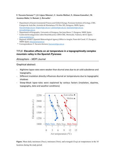
• Nighttime lapse rates were weaker than diurnal ones due to air cold subsidence processes and topography. Daily maximum air temperature lapse rates (LRmax) were steeper from March to July, although on the shady slope this only occurred around July. LRmax was weaker in winter. Daily minimum air temperature lapse rates (LRmin) were weaker from June to August (and December), and steeper from March to May.
• Different insolation values within and between the analyzed slopes were found, due to the facing slope and elevation of the locations, which directly influence diurnal air temperatures because of the topographic shadows in the valley bottom. This causes the retention of cold night air during the short days.
• Steep and weak lapse rate patterns were found, explained by various factors (slope insolation, daytime, topography, season and weather conditions). On clear winter days, the lower insolation of lower locations weakened LRmax. However, at this time, LRmax was steep under unstable atmospheric conditions. During the summer, LRmax was almost always steep (with few topographic shadows and mainly clear). LRmin was weak under stable atmospheric conditions, and steep under unstable ones, regardless of the month and season.

Our results support the fact that elevation is not a linear factor, as there are local variables that can alter the spatial and temporal distribution of air temperatures, so the selection of the measurement sites is crucial. This implies a need for rethinking when modeling air temperature at detailed scale, since it is important to analyze insolation, as well as vegetation cover, in addition to the effect of weather conditions. This work shows the need to analyze air temperature on a local scale when our applications need high spatial resolution.

References

- Bonnardot, V.; Carey, V.; Madelin, M.; Cautenet, S.; Coetzee, Z.; Quénol, H. Spatial variability of Night temperatures at a fine scale over the Stellenbosch Wine District, South Africa. J. Int. Sci. Vigne Vin 2012, 46, 1–13. [Google Scholar] [CrossRef] [Green Version]
- Hatfield, J.L.; Prueger, J.H. Temperature extremes: Effect on plant growth and development. Weather Clim. Extrem. 2015, 10, 4–10. [Google Scholar] [CrossRef] [Green Version]
- Tang, Z.; Fang, J. Temperature variation along the northern and southern slopes of Mt. Taibai, China. Agric. For. Meteorol. 2006, 139, 200–207. [Google Scholar] [CrossRef]
- Gilaberte-Búrdalo, M.; López-Martín, F.; Pino-Otín, M.R.; López-Moreno, J.I. Impacts of climate change on ski industry. Environ. Sci. Policy 2014, 44, 51–61. [Google Scholar] [CrossRef] [Green Version]
- Pons, M.; Johnson, P.; Rosas-Casals, M.; Sureda, B.; Jover, È. Modeling climate change effects on winter ski tourism in Andorra. Clim. Res. 2012, 54, 197–207. [Google Scholar] [CrossRef] [Green Version]
- Harlan, S.; Chowell, G.; Yang, S.; Petitti, D.; Morales Butler, E.; Ruddell, B.; Ruddell, D. Heat-Related Deaths in Hot Cities: Estimates of Human Tolerance to High Temperature Thresholds. Int. J. Environ. Res. Public Health 2014, 11, 3304–3326. [Google Scholar] [CrossRef] [Green Version]
- Barnett, T.P.; Adam, J.C.; Lettenmaier, D.P. Potential impacts of a warming climate on water availability in snow-dominated regions. Nature 2005, 438, 303–309. [Google Scholar] [CrossRef]
- Immerzeel, W.W.; Petersen, L.; Ragettli, S.; Pellicciotti, F. The importance of observed gradients of air temperature and precipitation for modeling runoff from a glacierized watershed in the Nepalese Himalayas. Water Resour. Res. 2014, 50, 2212–2226. [Google Scholar] [CrossRef] [Green Version]
- Pagès, M.; Miró, J.R. Determining temperature lapse rates over mountain slopes using vertically weighted regression: A case study from the Pyrenees. Meteorol. Appl. 2010, 17, 53–63. [Google Scholar] [CrossRef]
- García, M.B.; Domingo, D.; Pizarro, M.; Font, X.; Gómez, D.; Ehrlén, J. Rocky habitats as microclimatic refuges for biodiversity. A close-up thermal approach. Environ. Exp. Bot. 2019, 170, 1–10. [Google Scholar] [CrossRef]
- López-Moreno, J.I.; Navarro-Serrano, F.; Azorín-Molina, C.; Sánchez-Navarrete, P.; Alonso-González, E.; Rico, I.; Morán-Tejeda, E.; Buisán, S.; Revuelto, J.; Pons, M.; et al. Air and wet bulb temperature lapse rates and their impact on snowmaking in a Pyrenean ski resort. Theor. Appl. Climatol. 2019, 135, 1361–1373. [Google Scholar] [CrossRef]
- Ackerman, E.A. The Koppen Classification of Climates in North America. Geogr. Rev. 1941, 31, 105. [Google Scholar] [CrossRef]
- Villmow, J.R. Regional patterns of Climates in Europe according to the Thornthwaite Classification. Ohio J. Sci. 1962, 62, 39–53. [Google Scholar]
- Capel Molina, J.J. El Clima de la Península Ibérica; Ariel: Barcelona, Spain, 2000; p. 197. [Google Scholar]
- Whiteman, C.D.; Bian, X.; Zhong, S.; Whiteman, C.D.; Bian, X.; Zhong, S. Wintertime Evolution of the Temperature Inversion in the Colorado Plateau Basin. J. Appl. Meteorol. 1999, 38, 1103–1117. [Google Scholar] [CrossRef]
- Barry, R. Mountain Weather and Climate, 3rd ed.; Cambridge University Press: Cambridge, UK, 2008; ISBN 978-0-521-68158-2. [Google Scholar]
- Karki, R.; ul Hasson, S.; Schickhoff, U.; Scholten, T.; Böhner, J.; Gerlitz, L. Near surface air temperature lapse rates over complex terrain: A WRF based analysis of controlling factors and processes for the central Himalayas. Clim. Dyn. 2020, 54, 329–349. [Google Scholar] [CrossRef]
- Mahrt, L. Stratified atmospheric boundary layers and breakdown of models. Theor. Comput. Fluid Dyn. 1998, 11, 263–279. [Google Scholar] [CrossRef]
- Jiménez-Muñoz, J.C.; Sobrino, J.A. A generalized single-channel method for retrieving land surface temperature from remote sensing data. J. Geophys. Res. D Atmos. 2003, 108, 4688. [Google Scholar] [CrossRef] [Green Version]
- Khorchani, M.; Martin-Hernandez, N.; Vicente-Serrano, S.M.; Azorin-Molina, C.; Garcia, M.; Domínguez-Duran, M.A.; Reig, F.; Peña-Gallardo, M.; Domínguez-Castro, F. Average annual and seasonal Land Surface Temperature, Spanish Peninsular. J. Maps 2018, 14, 465–475. [Google Scholar] [CrossRef] [Green Version]
- Navarro-Serrano, F.; López-Moreno, J.I.; Domínguez-Castro, F.; Alonso-González, E.; Azorin-Molina, C.; El-Kenawy, A.; Vicente-Serrano, S.M. Maximum and minimum air temperature lapse rates in the Andean region of Ecuador and Peru. Int. J. Clim. 2020. [Google Scholar] [CrossRef]
- Geiger, R. The Climate near the Ground; Rowman & Littlefield Publishers: Lanham, MD, USA, 1965; ISBN 0742518574. [Google Scholar]
- Whiteman, C.D. Breakup of temperature inversions in deep mountain valleys: Part I. Observations. J. Appl. Meteorol. Clim. 1982, 21, 270–289. [Google Scholar] [CrossRef] [Green Version]
- Whiteman, C.D.; McKee, T.B. Breakup of temperature inversions in deep mountain valleys: Part II. Thermodynamic model. J. Appl. Meteorol. Clim. 1982, 21, 290–302. [Google Scholar] [CrossRef] [Green Version]
- Whiteman, C.D.; Zhong, S.; Shaw, W.J.; Hubbe, J.M.; Bian, X.; Mittelstadt, J. Cold Pools in the Columbia Basin. Weather 2001, 16, 432–447. [Google Scholar] [CrossRef] [Green Version]
- Lundquist, J.; Lott, F. Using inexpensive temperature sensors to monitor the duration and heterogeneity of snow-covered areas. Water Resour. Res. 2008, 44, 1–6. [Google Scholar] [CrossRef] [Green Version]
- Hubbart, J.; Kavanagh, K.; Pangle, R.; Link, T.; Schotzko, A. Cold air drainage and modeled nocturnal leaf water potential in complex forested terrain. Tree Physiol. 2007, 27, 631–639. [Google Scholar] [CrossRef] [PubMed] [Green Version]
- Minder, J.R.; Mote, P.W.; Lundquist, J.D. Surface temperature lapse rates over complex terrain: Lessons from the Cascade Mountains. J. Geophys. Res. Atmos. 2010, 115, 1–13. [Google Scholar] [CrossRef] [Green Version]
- Pepin, N.; Maeda, E.E.; Williams, R. Use of remotely sensed land surface temperature as a proxy for air temperatures at high elevations: Findings from a 5000 m elevational transect across Kilimanjaro. J. Geophys. Res. Atmos. 2016, 121, 9998–10015. [Google Scholar] [CrossRef] [Green Version]
- Kattel, D.B.; Yao, T.; Yang, W.; Gao, Y.; Tian, L. Comparison of temperature lapse rates from the northern to the southern slopes of the Himalayas. Int. J. Clim. 2015, 35, 4431–4443. [Google Scholar] [CrossRef]
- Hanna, E.; Mernild, S.; Yde, J.; Villiers, S. Surface Air Temperature Fluctuations and Lapse Rates on Olivares Gamma Glacier, Rio Olivares Basin, Central Chile, from a Novel Meteorological Sensor Network. Adv. Meteorol. 2017, 2017, 6581537. [Google Scholar] [CrossRef] [Green Version]
- Braun, M.; Hock, R. Spatially distributed surface energy balance and ablation modelling on the ice cap of King George Island (Antarctica). Glob. Planet. Chang. 2004, 42, 45–58. [Google Scholar] [CrossRef]
- Pagès, M.; Pepin, N.; Miró, J. Measurement and modelling of temperature cold pools in the Cerdanya valley (Pyrenees), Spain. Meteorol. Appl. 2017, 24, 290–302. [Google Scholar] [CrossRef] [Green Version]
- Miró, J.R.; Peña, J.C.; Pepin, N.; Sairouni, A.; Aran, M. Key features of cold-air pool episodes in the northeast of the Iberian Peninsula (Cerdanya, eastern Pyrenees). Int. J. Clim. 2017, 38, 1105–1115. [Google Scholar] [CrossRef]
- Benavides, R.; Montes, F.; Rubio, A.; Osoro, K. Geostatistical modelling of air temperature in a mountainous region of Northern Spain. Agric. For. Meteorol. 2007, 146, 173–188. [Google Scholar] [CrossRef]
- Navarro-Serrano, F.; López-Moreno, J.I.; Azorin-Molina, C.; Buisán, S.; Domínguez-Castro, F.; Sanmiguel-Vallelado, A.; Alonso-González, E.; Khorchani, M. Air temperature measurements using autonomous self-recording dataloggers in mountainous and snow covered areas. Atmos. Res. 2019, 224, 168–179. [Google Scholar] [CrossRef] [Green Version]
- Kulshrestha, S.; Ramsankaran, R. Investigating the performance of snowmelt runoff model using temporally varying near-surface lapse rate in Western Himalayas. Curr. Sci. 2018, 114, 808–813. [Google Scholar] [CrossRef]
- Heynen, M.; Miles, E.; Ragettli, S.; Buri, P.; Immerzeel, W.W.; Pellicciotti, F. Air temperature variability in a high-elevation Himalayan catchment. Ann. Glaciol. 2016, 57, 212–222. [Google Scholar] [CrossRef] [Green Version]
- Nigrelli, G.; Fratianni, S.; Zampollo, A.; Turconi, L.; Chiarle, M. The altitudinal temperature lapse rates applied to high elevation rockfalls studies in the Western European Alps. Theor. Appl. Climatol. 2017, 131, 1479–1491. [Google Scholar] [CrossRef]
- Marshall, S.J.; Sharp, M.J.; Burgess, D.O.; Anslow, F.S. Near-surface-temperature lapse rates on the Prince of Wales Icefield, Ellesmere Island, Canada: Implications for regional downscaling of temperature. Int. J. Clim. 2007, 27, 385–398. [Google Scholar] [CrossRef]
- Navarro-Serrano, F.; López-Moreno, J.; Azorin-Molina, C.; Alonso-González, E.; Tomás-Burguera, M.; Sanmiguel-Vallelado, A.; Revuelto, J.; Vicente-Serrano, S.M. Estimation of near-surface air temperature lapse rates over continental Spain and its mountain areas. Int. J. Clim. 2018, 38, 3233–3249. [Google Scholar] [CrossRef] [Green Version]
- Ojha, R. Identification of homogeneous regions of near surface air temperature lapse rates across India. Int. J. Clim. 2019, 39, 4288–4304. [Google Scholar] [CrossRef]
- Romshoo, S.A.; Rafiq, M.; Rashid, I. Spatio-temporal variation of land surface temperature and temperature lapse rate over mountainous Kashmir Himalaya. J. Mt. Sci. 2018, 15, 563–576. [Google Scholar] [CrossRef]
- Gardner, A.S.; Sharp, M.J.; Koerner, R.M.; Labine, C.; Boon, S.; Marshall, S.J.; Burgess, D.O.; Lewis, D. Near-Surface Temperature Lapse Rates over Arctic Glaciers and Their Implications for Temperature Downscaling. J. Clim. 2009, 22, 4281–4298. [Google Scholar] [CrossRef]
- Lookingbill, T.R.; Urban, D.L. Spatial estimation of air temperature differences for landscape-scale studies in montane environments. Agric. For. Meteorol. 2003, 114, 141–151. [Google Scholar] [CrossRef]
- Mahrt, L.; Vickers, D.; Nakamura, R.; Soler, M.R.; Sun, J.; Burns, S.; Lenschow, D.H. Shallow Drainage Flows. Bound. Layer Meteorol. 2001, 101, 243–260. [Google Scholar] [CrossRef]
- Soler, M.R.; Infante, C.; Buenestado, P.; Mahrt, L. Observations of Nocturnal Drainage Flow in a Shallow Gully. Bound. Layer Meteorol. 2002, 105, 253–273. [Google Scholar] [CrossRef]
- Barry, R.; Chorley, R. Atmosphere, Weather and Climate, 1st ed.; Taylor & Francis: Abingdon, UK, 1987; p. 536. [Google Scholar]
- Von Arx, G.; Dobbertin, M.; Rebetez, M. Spatio-temporal effects of forest canopy on understory microclimate in a long-term experiment in Switzerland. Agric. For. Meteorol. 2012, 166–167, 144–155. [Google Scholar] [CrossRef]
- Lareau, N.P.; Horel, J.D. Dynamically Induced Displacements of a Persistent Cold-Air Pool. Bound. Layer Meteorol. 2014, 154, 291–316. [Google Scholar] [CrossRef] [Green Version]
- Moron, V.; Oueslati, B.; Pohl, B.; Janicot, S. Daily Weather Types in February–June (1979–2016) and Temperature Variations in Tropical North Africa. J. Appl. Meteorol. Clim. 2018, 57, 1171–1195. [Google Scholar] [CrossRef]
- Kirchner, M.; Faus-Kessler, T.; Jakobi, G.; Leuchner, M.; Ries, L.; Scheel, H.-E.; Suppan, P. Altitudinal temperature lapse rates in an Alpine valley: Trends and the influence of season and weather patterns. Int. J. Clim. 2013, 33, 539–555. [Google Scholar] [CrossRef]
- García-Ruiz, J.M.; López-Moreno, J.I.; Vicente-Serrano, S.M.; Lasanta–Martínez, T.; Beguería, S. Mediterranean water resources in a global change scenario. Earth Sci. Rev. 2011, 105, 121–139. [Google Scholar] [CrossRef] [Green Version]
- Lasanta, T.; Laguna, M.; Vicente-Serrano, S.M. Do tourism-based ski resorts contribute to the homogeneous development of the Mediterranean mountains? A case study in the Central Spanish Pyrenees. Tour. Manag. 2007, 28, 1326–1339. [Google Scholar] [CrossRef]
- Morán-Tejeda, E.; Herrera, S.; López-Moreno, J.I.; Revuelto, J.; Lehmann, A.; Beniston, M. Evolution and frequency (1970–2007) of combined temperature–precipitation modes in the Spanish mountains and sensitivity of snow cover. Reg. Environ. Chang. 2013, 13, 873–885. [Google Scholar] [CrossRef] [Green Version]
- López-Moreno, J.I.; García-Ruiz, J.M. Influence of snow accumulation and snowmelt on streamflow in the central Spanish Pyrenees. Hydrol. Sci. J. 2004, 49, 787–801. [Google Scholar] [CrossRef]
- López-Moreno, J.I.; Gascoin, S.; Herrero, J.; Sproles, E.A.; Pons, M.; Alonso-González, E.; Hanich, L.; Boudhar, A.; Musselman, K.N.; Molotch, N.P.; et al. Different sensitivities of snowpacks to warming in Mediterranean climate mountain areas. Environ. Res. Lett. 2017, 12, 074006. [Google Scholar] [CrossRef]
- Esteban, P.; Ninyerola, M.; Prohom, M. Spatial modelling of air temperature and precipitation for Andorra (Pyrenees) from daily circulation patterns. Theor. Appl. Climatol. 2009, 96, 43–56. [Google Scholar] [CrossRef]
- Buisán, S.; Saz, M.A.; López-Moreno, J.I.; López-Moreno, J.I. Spatial and temporal variability of winter snow and precipitation days in the western and central Spanish Pyrenees. Int. J. Clim. 2015, 35, 259–274. [Google Scholar] [CrossRef]
- Alonso-González, E.; López-Moreno, J.I.; Navarro-Serrano, F.; Sanmiguel-Vallelado, A.; Revuelto, J.; Domínguez-Castro, F.; Ceballos, A. Snow climatology for the mountains in the Iberian Peninsula using satellite imagery and simulations with dynamically downscaled reanalysis data. Int. J. Clim. 2020, 40, 477–491. [Google Scholar] [CrossRef]
- López-Moreno, J.I.; Vicente-Serrano, S.M.; Moran-Tejeda, E.; Zabalza, J.; Lorenzo-Lacruz, J.; García-Ruiz, J.M. Impact of climate evolution and land use changes on water yield in the ebro basin. Hydrol. Earth Syst. Sci. 2011, 15, 311–322. [Google Scholar] [CrossRef] [Green Version]
- Esteban-Parra, M.J.; Rodrigo, F.S.; Castro-Diez, Y. Spatial and temporal patterns of precipitation in Spain for the period 1880–1992. Int. J. Clim. 1998, 18, 1557–1574. [Google Scholar] [CrossRef]
- Agencia Estatal de Meteorología (AEMET); Ministerio de Medio Ambiente y Medio Rural y Marino; Instituto de Meteorología de Portugal. Atlas Climático Ibérico, 1st ed.; Closas-Orcoyen, S.L.: Madrid, Spain, 2011.
- Crespo, D.; Albiac, J.; Kahil, T.; Esteban, E.; Baccour, S. Tradeoffs between Water Uses and Environmental Flows: A Hydroeconomic Analysis in the Ebro Basin. Water Resour. Manag. 2019, 33, 2301–2317. [Google Scholar] [CrossRef] [Green Version]
- García-Garizábal, I.; Causapé, J.; Merchán, D. Evaluation of alternatives for flood irrigation and water usage in Spain under Mediterranean climate. Catena 2017, 155, 127–134. [Google Scholar] [CrossRef] [Green Version]
- Buisán, S.; López-Moreno, J.; Saz, M.; Kochendorfer, J. Impact of weather type variability on winter precipitation, temperature and annual snowpack in the Spanish Pyrenees. Clim. Res. 2016, 69, 79–92. [Google Scholar] [CrossRef]
- Navarro-Serrano, F.; López-Moreno, J.I. Spatio-temporal analysis of snowfall events in the Spanish Pyrenees and ther relationship to atmospheric circulation. Cuad. Investig. Geográfica 2017, 43, 233–254. [Google Scholar] [CrossRef] [Green Version]
- Nadal-Romero, E.; Cammeraat, E.; Pérez-Cardiel, E.; Lasanta, T. Effects of secondary succession and afforestation practices on soil properties after cropland abandonment in humid Mediterranean mountain areas. Agric. Ecosyst. Environ. 2016, 228, 91–100. [Google Scholar] [CrossRef] [Green Version]
- Pueyo, Y.; Beguería, S. Modelling the rate of secondary succession after farmland abandonment in a Mediterranean mountain area. Landsc. Urban Plan. 2007, 83, 245–254. [Google Scholar] [CrossRef] [Green Version]
- Buisán, S.; Azorin-Molina, C.; Jimenez, Y. Impact of two different sized Stevenson screens on air temperature measurements. Int. J. Clim. 2015, 35, 4408–4416. [Google Scholar] [CrossRef]
- Imholt, C.; Soulsby, C.; Malcolm, I.; Hrachowitz, M.; Gibbins, C.; Langan, S.; Tetzlaff, D. Influence of Scale on Thermal characteristics in a large montane River Basin. River Res. Appl. 2013, 29, 403–419. [Google Scholar] [CrossRef]
- Yang, Z.; Hanna, E.; Callaghan, T.; Jonasson, C. How can meteorological observations and microclimate simulations improve understanding of 1913–2010 climate change around Abisko, Swedish Lapland? Meteorol. Appl. 2012, 19, 454–463. [Google Scholar] [CrossRef]
- Pepin, N.; Kidd, D. Spatial temperature variation in the Eastern Pyrenees. Weather 2006, 61, 300–310. [Google Scholar] [CrossRef]
- Serrano, E.; Sanjosé-Blasco, J.J.; Gómez-Lende, M.; López-Moreno, J.I.; Pisabarro, A.; Martínez-Fernández, A. Periglacial environments and frozen ground in the central Pyrenean high mountain area: Ground thermal regime and distribution of landforms and processes. Permafr. Periglac. Process. 2019, 30, 292–309. [Google Scholar] [CrossRef]
- Rolland, C. Spatial and Seasonal Variations of Air Temperature Lapse Rates in Alpine Regions. J. Clim. 2003, 16, 1032–1046. [Google Scholar] [CrossRef] [Green Version]
- Du, M.; Liu, J.; Zhang, X.; Li, Y.; Tang, Y. Changes of spatial patterns of surface-air-temperature on the Tibetan Plateau. Latest Trends Theor. Appl. Mech. Fluid Mech. Heat Mass Transf. 2010, 47, 42–47. [Google Scholar]
- Blandford, T.R.; Humes, K.S.; Harshburger, B.J.; Moore, B.C.; Walden, V.P.; Ye, H. Seasonal and Synoptic Variations in Near-Surface Air Temperature Lapse Rates in a Mountainous Basin. J. Appl. Meteorol. Clim. 2008, 47, 249–261. [Google Scholar] [CrossRef]
- Florinsky, I.V.; Kulagina, T.B.; Meshalkina, J.L. Influence of topography on landscape radiation temperature distribution. Int. J. Remote Sens. 1994, 15, 3147–3153. [Google Scholar] [CrossRef]
- IGN Plan Nacional de Ortofotografía Aérea. Available online: https://pnoa.ign.es/presentacion-y-objetivo (accessed on 27 January 2020).
- Corripio, J.G. Insol: Solar Radiation. R Package Version 1.2.1. Available online: https://CRAN.R-project.org/package=insol. (accessed on 20 May 2020).
- R Core-Team. R: A Language and Environment for Statistical Computing 2013; R Foundation for Statistical Computing: Vienna, Austria, 2013. [Google Scholar]
- Jenkinson, A.F.; Collison, P. An initial climatology of Wales over the North Sea. In Synoptic Climatology Branch Memorandum; Meteorological Office: Bracknell, UK, 1997; p. 62. [Google Scholar]
- Lamb, H.H. British Isles weather types and a register of daily sequence of circulation patterns, 1861–1971. Geophys. Mem. 1972, 116, 85. [Google Scholar]
- Rasilla Álvarez, D.F.; García-Codrón, J.C.; Garmendia Pedraja, C. Los temporales de viento: Propuesta metodológica para el análisis de un fenómeno infravalorado. In Proceedings of the 7th Reunión Nacional de Climatología, Albarracin, Spain, 27–29 June 2002; pp. 129–136. [Google Scholar]
- Basnett, T.A.; Parker, D.E. Development of the global mean sea level pressure data set GMSLP2. In Climatic Research Technical Note; Hadley Centre, Meteorological Office: Bracknell, UK, 1997; Volume 79. [Google Scholar]
- Charrad, M.; Ghazaali, N.; Boiteau, V.; Niknafs, A. NbClust: An R package for determining the relevant number of clusters in a data Set. J. Stat. Softw. 2014, 61, 1–36. [Google Scholar] [CrossRef] [Green Version]
- Murtagh, F.; Legendre, P. Ward’s Hierarchical Agglomerative Clustering Method: Which Algorithms Implement Ward’s Criterion? J. Classif. 2014, 31, 274–295. [Google Scholar] [CrossRef] [Green Version]
- Wilcoxon, F. Individual Comparisons by Ranking Methods. Biom. Bull. 1945, 1, 80. [Google Scholar] [CrossRef]
- Ninyerola, M.; Pons, X.; Roure, J.M. A methodological approach of climatological modelling of air temperature and precipitation through GIS techniques. Int. J. Clim. 2000, 20, 1823–1841. [Google Scholar] [CrossRef]
- Espín-Sánchez, E.; Ruiz-Álvarez, V.; Martí-Talavera, J.; García-Marín, R. Estudio preliminar de las inversiones térmicas en el sureste de la Península Ibérica: El caso de los campos de Hernán Perea. Pirin. Rev. Ecol. Montaña. 2018, 173, 1–18. [Google Scholar]
- Daly, C.; Gibson, W.; Taylor, G.; Johnson, G.; Pasteris, P. A knowledge-based approach to the statistical mapping of climate. Clim. Res. 2002, 22, 99–113. [Google Scholar] [CrossRef] [Green Version]
- Sadoti, G.; McAfee, S.A.; Roland, C.A.; Fleur Nicklen, E.; Sousanes, P.J. Modelling high-latitude summer temperature patterns using physiographic variables. Int. J. Clim. 2018, 38, 4033–4042. [Google Scholar] [CrossRef]
- Lundquist, J.D.; Pepin, N.; Rochford, C. Automated algorithm for mapping regions of cold-air pooling in complex terrain. J. Geophys. Res. 2008, 113, 1–15. [Google Scholar] [CrossRef] [Green Version]
- Pepin, N. Lapse rate changes in northern England. Theor. Appl. Climatol. 2001, 68, 1–16. [Google Scholar] [CrossRef]
- Price, J.D.; Vosper, S.; Brown, A.; Ross, A.; Clark, P.; Davies, F.; Horlacher, V.; Claxton, B.; McGregor, J.R.; Hoare, J.S.; et al. Colpex: Field and numerical studies over a region of small hills. Bull. Am. Meteorol. Soc. 2011, 92, 1636–1650. [Google Scholar] [CrossRef] [Green Version]
- Du, M.; Zhang, M.; Wang, S.; Zhu, X.; Che, Y. Near-surface air temperature lapse rates in Xinjiang, northwestern China. Theor. Appl. Climatol. 2017, 131, 1–14. [Google Scholar] [CrossRef]
- Sanmiguel-Vallelado, A.; López-Moreno, J.I.; Morán-Tejeda, E.; Alonso-González, E.; Navarro-Serrano, F.; Rico, I.; Camarero, J.J. Variable effects of forest canopies on snow processes in a valley of the central Spanish Pyrenees. Hydrol. Process. 2020, 34, 2247–2262. [Google Scholar] [CrossRef]
- Barringer, J.R.F. A variable lapse rate snowline model for the Remarkables, Central Otago, New Zealand. J. Hydrol. 1989, 28, 32–46. [Google Scholar]
- Duane, W.J.; Pepin, N.C.; Losleben, M.L.; Hardy, D.R. General characteristics of Temperature and Humidity Variability on Kilimanjaro, Tanzania. Arct. Antarct. Alp. Res. 2008, 40, 323–334. [Google Scholar] [CrossRef]
- Dumas, M.D. Changes in temperature and temperature gradients in the French Northern Alps during the last century. Theor. Appl. Climatol. 2013, 111, 223–233. [Google Scholar] [CrossRef] [Green Version]
- Dodson, R.; Marks, D. Daily air temperature interpolated at high spatial resolution over a large mountainous region. Clim. Res. 1997, 8, 1–20. [Google Scholar] [CrossRef]
- Joshi, R.; Sambhav, K. Near surface temperature lapse rate for treeline environment in western Himalaya and possible impacts on ecotone vegetation. Trop. Ecol. 2018, 59, 197–209. [Google Scholar] [CrossRef]
- Lareau, N.P.; Crosman, E.; Whiteman, C.D.; Horel, J.D.; Hoch, S.W.; Brown, W.O.J.; Horst, T.W. The Persistent Cold-Air Pool Study. Bull. Am. Meteorol. Soc. 2013, 94, 51–63. [Google Scholar] [CrossRef] [Green Version]
- Bolstad, P.V.; Swift, L.; Collins, F.; Régnière, J. Measured and predicted air temperatures at basin to regional scales in the southern Appalachian mountains. Agric. For. Meteorol. 1998, 91, 161–176. [Google Scholar] [CrossRef]