Possible Link Between Arctic Sea Ice and January PM₁₀ Concentrations in South Korea

Abstract

In this study, we investigated the possible teleconnection between PM₁₀ concentrations in South Korea and Arctic Sea ice concentrations at inter-annual time scales using observed PM₁₀ data from South Korea, NCEP R2 data, and NOAA Sea Ice Concentration (SIC) data from 2001 to 2018. From the empirical orthogonal function (EOF) analysis, we found that the first mode (TC1) was a large-scale mode for PM₁₀ in South Korea and explained about 27.4% of the total variability. Interestingly, the TC1 is more dominantly influenced by the horizontal ventilation effect than the vertical atmospheric stability effect. The pollution potential index (PPI), which is defined by the weighted average of the two ventilation effects, is highly correlated with the TC1 of PM₁₀ at a correlation coefficient of 0.75, indicating that the PPI is a good measure for PM₁₀ in South Korea at inter-annual time scales. Regression maps show that the decrease of SIC over the Barents Sea is significantly correlated with weakening of high pressure over the Ural mountain range region, the anomalous high pressure at 500 hPa over the Korean peninsula, and the weakening of the Siberian High and Aleutian low. Moreover, these patterns are similar to the correlation pattern with the PPI, suggesting that the variability of SIC over the Barents Sea may play an important role in modulating the variability of PM₁₀ in South Korea through teleconnection from the Barents Sea to the Korean peninsula via Eurasia.

1. Introduction

In recent years, there have been strong and frequent occurrences of high concentrations of particulate matter (PM) pollution over East Asia [1,2,3,4,5]; PM-related damages have occurred in many countries. In particular, in January 2013, China suffered tremendous damage due to an unprecedented high concentration of PM pollution [1,6,7]. With a rise in damage from high concentrations of PM pollution came an increased interest in the mechanisms causing them.

Particulate matter with a diameter < 10 µm (PM₁₀) floating in the atmosphere is common in emissions from factories, cars, and burning fossil fuels [8]. Owing to implementation of the reduction policy of domestic pollutant emissions [9,10,11], the PM₁₀ concentration in South Korea is steadily decreasing; however, high concentration PM₁₀ events continue to frequently take place [3]. South Korea is a region where high concentrations of pollutants occur due to a combination of air pollutants coming from neighboring countries and originating domestically [12]. According to previous studies, high concentrations of PM₁₀ in South Korea can be caused by anomalous high pressure in the upper atmosphere over the Korean peninsula or by transport from the source of major PM [3,13,14]. Recent studies have also showed that changes in atmospheric circulation patterns due to climate change can increase concentrations of fine dust particles [1,3,6]. Wie and Moon [15] showed that ENSO-affected weather conditions in winter can affect the variation of PM₁₀ concentrations in South Korea. In particular, Zou et al. [7] suggested that atmospheric ventilation plays an important role in extreme winter haze event in the East China Plain (ECP), and the haze in the ECP during winter is related to the Arctic sea ice loss in the preceding autumn and Eurasian snowfall in the earlier winter. However, Shen et al. [16] stressed that there were no significant correlations between the Arctic sea ice loss and winter haze in northern China. Instead, they found that winter haze was significantly correlated with both wind speed and relative humidity. Zhao et al. [6] suggested that low pollution concentrations in North China Plain can originate from strong Siberian High due to the warming Arctic and the reducing SIC in the past decades.

In Korea, January PM₁₀ concentration and its inter-annual variability are relatively high, compared to other months. However, the possible impact of Arctic sea ice forcing on January PM₁₀ concentration in South Korea remains uncertain at the inter-annual time scale. Therefore, this study examines the inter-annual variability of January PM₁₀ concentrations in South Korea and the NH (northern hemisphere) circulation patterns favorable for high PM₁₀ in the country, as well as the associated Arctic sea ice forcing in the NH.

2. Data and Methods

2.1. Data

In this study, we used monthly PM₁₀ data for 18 years (2001 to 2018) from 68 observational stations provided by the National Institute of Environmental Research (South Korea). For statistical reliability of data, monthly mean values were calculated only when more than 70% of the daily data are available during the analysis period; 68 observational stations were selected as valid inputs (Figure 1).

The characteristics of atmospheric circulation in the NH affecting inter-annual variability of PM₁₀ concentrations on the Korean Peninsula were analyzed using National Centers for Environmental Prediction-National Center for Atmospheric Research Reanalysis 2 (NCEP R2) data for 40 years (1979 to 2018), with a horizontal resolution of 2.5° × 2.5°. The major variables used were monthly mean geopotential height and horizontal winds at 1000, 500, and 250 hPa, and sea level pressure and surface air temperature.

In this study, we used Optimum Interpolation Sea Surface temperature (OISST) version 2′s Sea Ice Concentration (SIC) data provided by National Oceanic and Atmospheric Administration (NOAA) to analyze the climatic factors affecting PM₁₀ concentrations in South Korea. The analysis period for the SIC is 37 years (1982 to 2018), with a horizontal resolution of 1° × 1° in the NH.

2.2. Methods

In this study, two ventilation effects were considered as large-scale factors affecting the inter-annual variability of PM₁₀ concentrations in South Korea. The first is wind speed representing the horizontal ventilation effect, and the second is atmospheric stability representing the vertical ventilation effect. In this study, two ventilation indices were calculated using the method presented in Zou et al. [7]. A near-surface wind speed index (WSI) was defined by normalizing the horizontal wind speed of 1000 hPa as the horizontal ventilation effect. A potential air temperature gradient index (ATGI) was defined by normalizing the potential air temperature gradient between 925 hPa and 1000 hPa as the vertical ventilation effect. The PPI was defined by the weighted averaging of the two effects using the correlation coefficient between the two ventilation indices and the PM₁₀ concentration to take into account the effects of both ventilation indices (Equation (1) to (4)). The three ventilation indices for South Korea were obtained by normalizing the area average values for South Korea (33–38° N, 125–120° E) as follows:

$${\mathrm{ATGI}}_i^j=\left({\mathrm{ATG}}_i^j-{\mathrm{ATG}}_{\mathrm{mean}}^j\right)/{\mathrm{ATG}}_{\mathrm{std}}^j,$$

(1)

$${\mathrm{WSI}}_i^j=\left({\mathrm{WS}}_i^j-{\mathrm{WS}}_{\mathrm{mean}}^j\right)/{\mathrm{WS}}_{\mathrm{std}}^j,$$

(2)

$${\mathrm{NWSI}}_i^j=-{\mathrm{WSI}}_i^j,$$

(3)

$${\mathrm{PPI}}_i^j=\frac{r_1\times {\mathrm{WSI}}_i^j+r_2\times {\mathrm{ATGI}}_i^j}{\left|r_1\right|+\left|r_2\right|},$$

(4)

where i is time, j is each grid, and the subscripts mean and std indicate the climatological mean and standard deviation for the analysis period. r₁ and r₂ are the correlation coefficients between PM₁₀ and the ventilation indices (WSI and ATGI) in South Korea. In addition, we also defined NWSI by multiplying the negative value to WSI for ease of interpretation. As the ATGI and NWSI increase, the ventilation effect decreases, resulting in higher air pollution concentrations. Thus, the PPI is a good indicator of the degree of pollution concentration in South Korea.

It is well known that sea ice concentrations over the Arctic are strongly linked to the circulation pattern over the mid-latitudes, i.e., Ural blocking and Siberian High [17,18,19]. This means that the variability of sea ice over the Arctic may influence the variability of PM₁₀ in South Korea through changes in atmospheric circulation and associated ventilation effects. In this study, we found a core region around the Barents Sea where sea ice concentration strongly correlated with the variability of PM₁₀ in South Korea. Thus, we defined Sea Ice Index (SII) as the normalized Sea Ice Concentration (SIC) over the Barents Sea with a statistically significant correlation with the PM₁₀ concentration in South Korea (Equation (5)). For convenience, we also defined negative SII (NSII) by multiplying the negative value with the SII (Equation (6)). We also defined Arctic SII (ASII) for the Arctic ocean (over 60° N) in Equation (7). It should be noted that the linear trend of the SIC was removed before statistical analysis. See Section 3.3 in detail.

$${\mathrm{SII}}_i^j=\left({\mathrm{SIC}}_i^j-{\mathrm{SIC}}_{\mathrm{mean}}^j\right)/{\mathrm{SIC}}_{\mathrm{std}}^j,$$

(5)

$${\mathrm{NSII}}_i^j=-{\mathrm{SII}}_i^j,$$

(6)

$${\mathrm{ASII}}_i^j=\left({\mathrm{ASIC}}_i^j-{\mathrm{ASIC}}_{\mathrm{mean}}^j\right)/{\mathrm{ASIC}}_{\mathrm{std}}^j,$$

(7)

3. Results

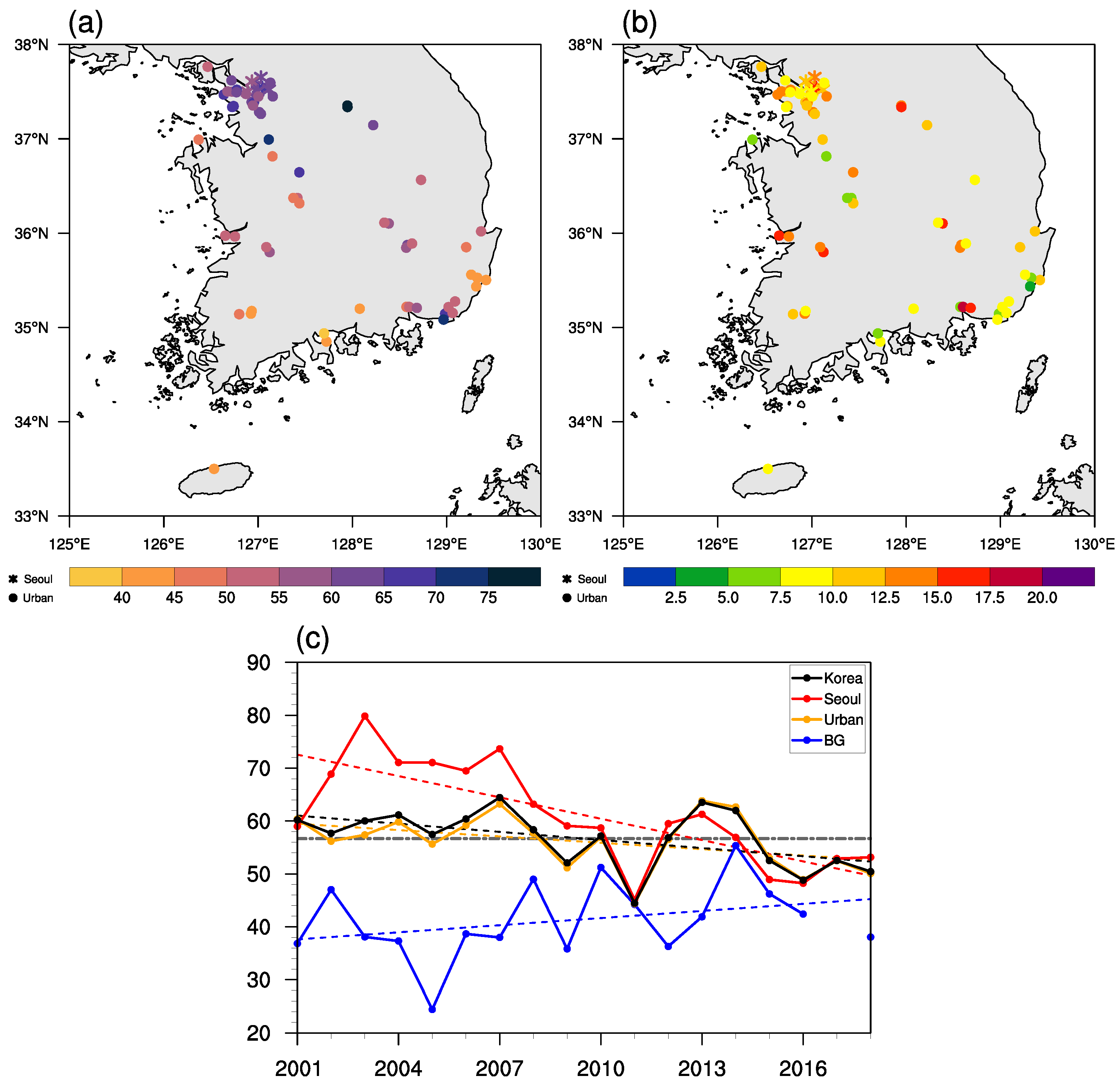
3.1. Inter-Annual Variability of PM₁₀ Concentrations in South Korea

In Korea, high PM₁₀ concentrations occur in the spring and winter seasons, mainly due to yellow dust and the combustion of heating fuel [3,14]. There have recently been frequent observations of high concentrations of PM₁₀ in China and Korea in the month of January [3,7]. Figure 1 shows the climatological mean and standard deviation of PM₁₀ concentration in each station in South Korea. The climatological mean PM₁₀ concentration in January was about 57 μg/m³ in South Korea, 61 μg/m³ in Seoul, and 41 μg/m³ at a background station, with high PM₁₀ concentrations and high variability over metropolitan areas, including Seoul and Incheon. Interestingly the observations from Seoul showed a strongly linear decreasing tendency over time, while the background station showed a slightly linear increasing trend (Figure 1c,

Table 1. Linear trend coefficient for each station in South Korea. Superscripts indicate significance at the 99%, 95%, and 90% confidence levels, respectively.

	Trend (µg/m3 Per Total Period)	Note
Seoul	−24.2 ***	During 2001–2018
Urban	−7.2 *
All stations	−9.2 **
Background	8.1	Without 2017(2001–2018)
	10.4	During 2001–2016

* 90%, ** 95%, *** 99% confidence level.

). The linear decline trend in Seoul and major cities can be attributed to the emission reduction policy implemented by the Korean government [10,11]. Climate change and associated circulation change also contribute to the trend of PM₁₀ concentrations in South Korea. Therefore, in order to focus only on the inter-annual variability of PM₁₀ concentrations in South Korea, we performed an analysis by removing the linear trend for each station in the analysis period.

It is unclear if the inter-annual variability of PM₁₀ in South Korea can be controlled by the large-scale mode or not. In order to extract the large-scale mode from the data, we applied Empirical orthogonal function (EOF) analysis to the PM₁₀ data in South Korea. The first mode of EOF explained about 27.4% of the total variation, and eigenvectors of the same sign appeared in all stations (Figure 2), indicating that this mode is controlled by large-scale factors rather than local ones. In particular, the time coefficient (TC) of the first mode showed a positive peak in 2013, 2014, and 2007, and a negative peak in 2011. These peaks are in good agreement with the high concentration cases and low concentration cases in South Korea, as shown in Figure 1. Therefore, we defined this first mode as the large-scale mode and named it TC1. On the other hand, the second EOF mode of PM₁₀ concentrations in South Korea appeared to be linear and explained about 16.1% of the total variation (not shown).

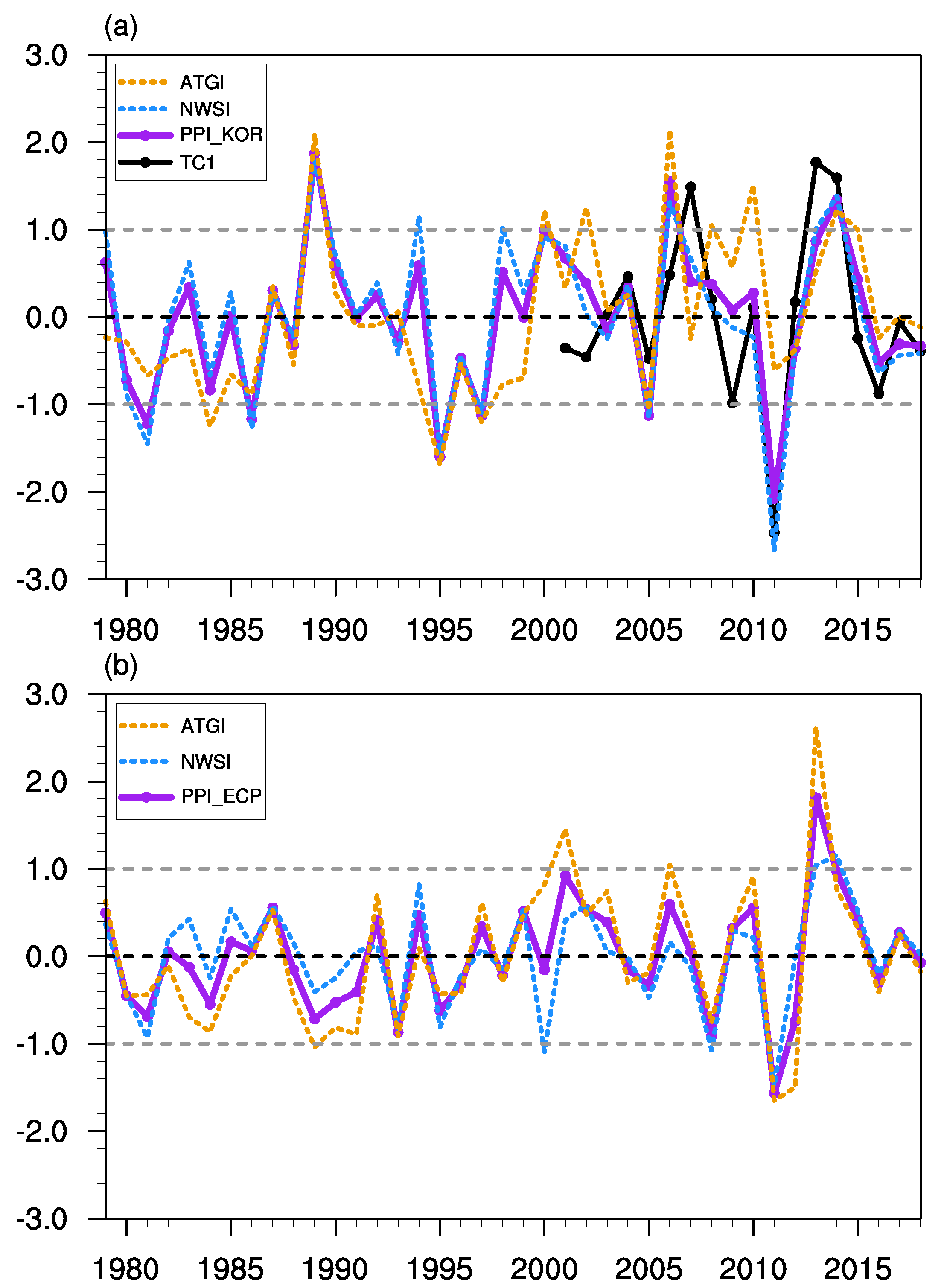
3.2. Relationship between PM₁₀ and Ventilation Indices in South Korea

PM₁₀ concentration at daily time scales is influenced by various weather factors, such as atmospheric vertical stability, horizontal wind velocity, wind direction, deposition, and mixing height, among others. Zou et al. [7] showed that in the ECP region, the atmospheric vertical stability index (correlation coefficient r = 0.73) and the horizontal ventilation index (r = 0.70) have similar effects on the PM₁₀ concentration inter-annual time scale (

Table 2. Correlation coefficients between TC1 (time coefficient (TC) of the first mode) and various indices in South Korea compared with the ECP (East China Plain) region of China. Superscripts indicate significance at the 99%, 95% confidence levels, respectively. (ATGI: air temperature gradient index; NWSI: negative value of wind speed index; PPI: pollution potential index).

CORR	ATGI	NWSI	PPI	Note
KOREA	0.34	0.82 ***	0.75 ***	This study
ECP	0.70**	0.73 ***	0.92 ***	Zou et al. [7]

** 95%, *** 99% confidence level.

). However, the PM₁₀ concentration in South Korea is more significantly influenced by the horizontal ventilation effect (r = 0.82) than atmospheric vertical stability (r = 0.34) (Table 2). There is a clear difference in the meteorological factors affecting PM₁₀ concentration in the ECP region and the Korean peninsula.

As shown in previous studies, the rise in northerly wind in certain high-density episodes could increase the concentration of PM₁₀ in South Korea by propelling the transport of pollutants originating from northern China [3,10,13,14]. However, the analysis of this study clearly shows that PM₁₀ concentration increases when January wind (mostly northerly wind) speed decreases (Table 2). This means that the weakening of northerly wind at the inter-annual time scale contributes to the reduction of diffusion rather than to the decrease of pollutant transport originating from China. In other words, when wind speed becomes stronger, the curtain effect not only blocks the transport of pollutants originating from the ECP region, but also increases horizontal diffusion, lessening PM₁₀ concentrations. In addition, the effect of stability on PM₁₀ concentration in South Korea is considerably weaker than that of the ECP region (Table 2). The ECP area is basin-shaped, and the air masses originating from the Tibetan Plateau contribute to an increase in stability because they induce downdrafts at upper troposphere over the ECP area.

The Korean peninsula is mainly influenced by dynamic factors rather than thermal factors. As explained earlier, the Pollution Potential Index (PPI) was calculated by the linear combination of two atmospheric ventilation indices, using the correlation coefficient with the atmospheric ventilation index and the TC1 in South Korea (Figure 3). Zou et al. [7] found that the correlation between PPI and PM₁₀ concentrations in the ECP region was 0.92, which is statistically significant to 1%. The PPI in South Korea showed a correlation of 0.75 with TC1, which was statistically significant to 1%. Time series of PPIs in these two regions match well with peak values in 2013 and minimum in 2011 of PM₁₀ concentrations (Figure 3), indicating that the PPI is an effective index suitable for diagnosing PM₁₀ contamination concentrations in South Korea. These results also indicate that there is a clear difference in the relative contribution of the meteorological factors affecting PM₁₀ concentrations in the ECP region and South Korea, as explained in Figure 4 and Figure 5.

To identify the inter-annual variability of PPI in South Korea and the atmospheric circulation of the NH, we performed a correlation analysis of PPI and large-scale atmospheric fields (Figure 4). The PPI of South Korea showed a positive correlation with the geopotential height at 500 hPa over the Korean peninsula region, and a strong negative correlation was found over northern Eurasia, including the Ural mountain range region. The north-south dipole correlation pattern in the geopotential height at 500 hPa corresponds to the intensification of the jet stream at 500 hPa over the region between negative correlation and positive correlation zones, spanning from the Caspian Sea to Hokkaido in Japan. This indicates that intensified jet stream blocks cold air from the Arctic, resulting in warming in South Korea. Moreover, the correlation map between sea level pressure (SLP) and PPI shows an east-west pattern, which results in a weakening of Siberian high and Aleutian low and thereby a weakening of wind speed over the Korean peninsula. In other words, the relative weakening of high pressure over the Ural mountain range region and the anomalous high pressure in the Korean peninsula strengthen the jet stream to the north of the Korean peninsula. As a result, the strong inflow of cold air from the north to the Korean peninsula is blocked and the weak northerly flow prevents air from ventilating over the Korean peninsula, resulting in high PM₁₀ concentrations.

On the other hand, the PPI in the ECP region is partly different from that in South Korea. The PPI in the ECP region is strongly correlated to the Siberian high, but not with the Aleutian low (Figure 5). However, the PPI in South Korea is strongly correlated to both the Siberian high and the Aleutian low, especially in the center of the Siberian high and in the southwestern edge of the Aleutian low (Figure 4), indicating that the pressure gradient force around the South Korea is stronger than in the ECP region.

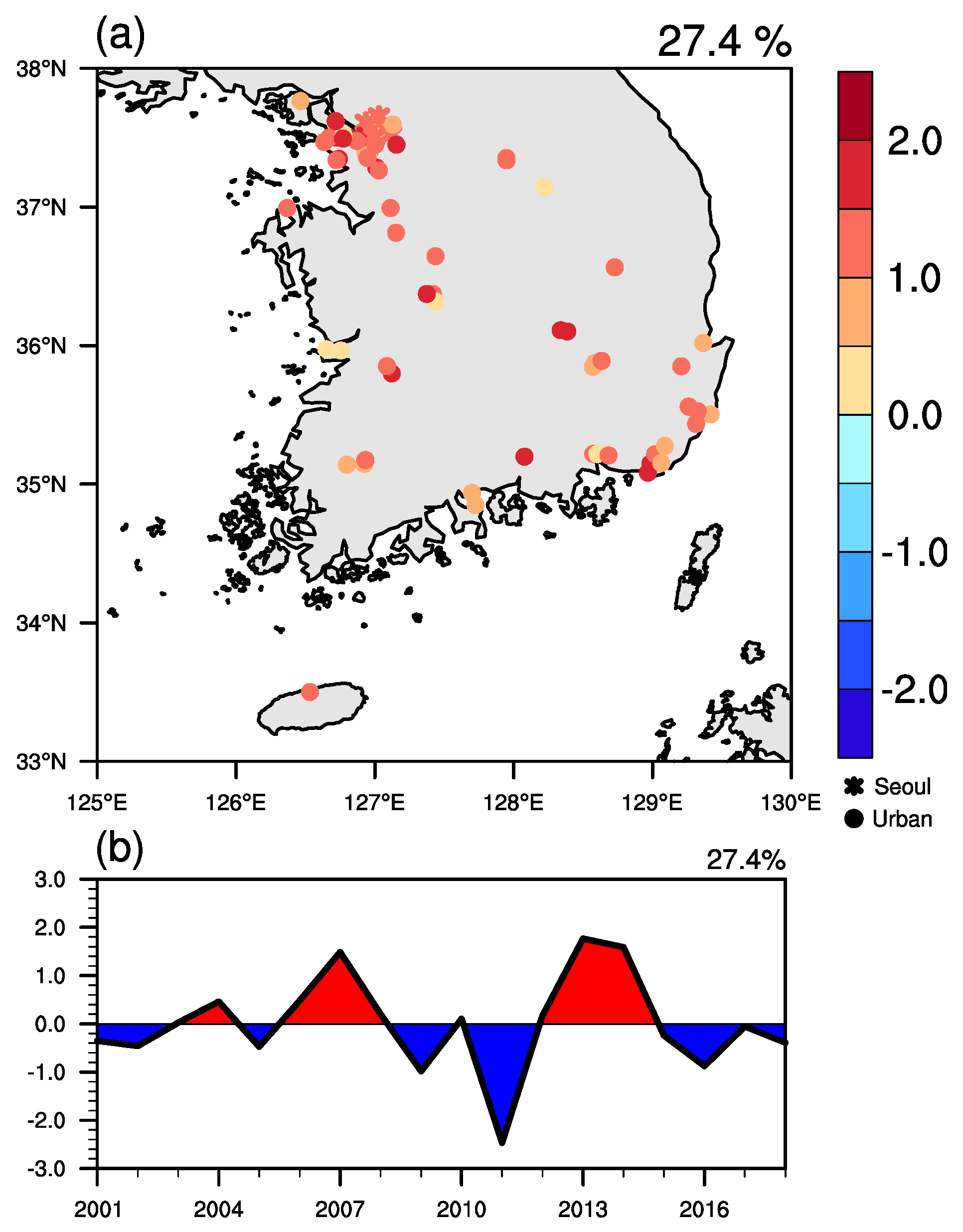
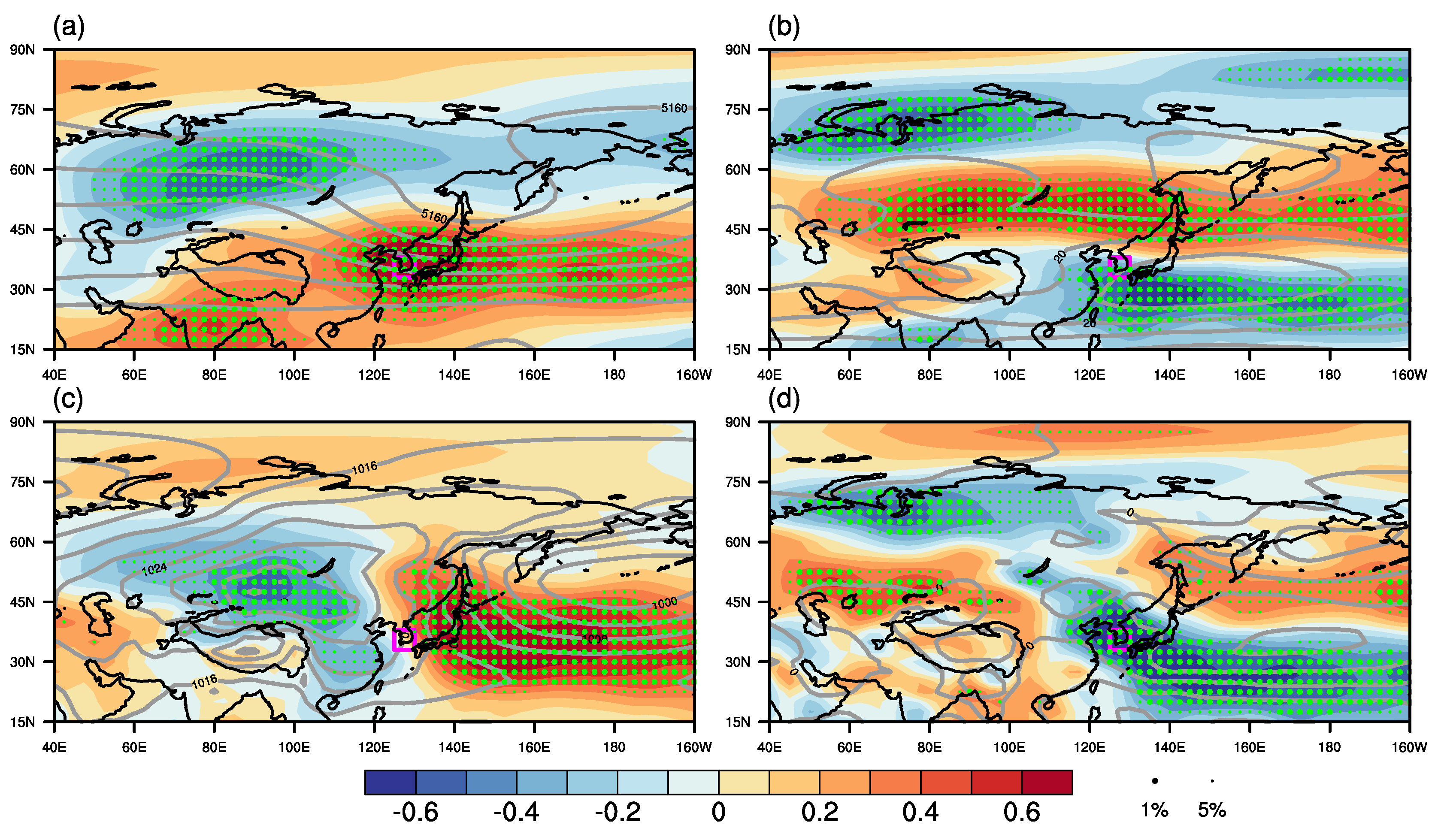
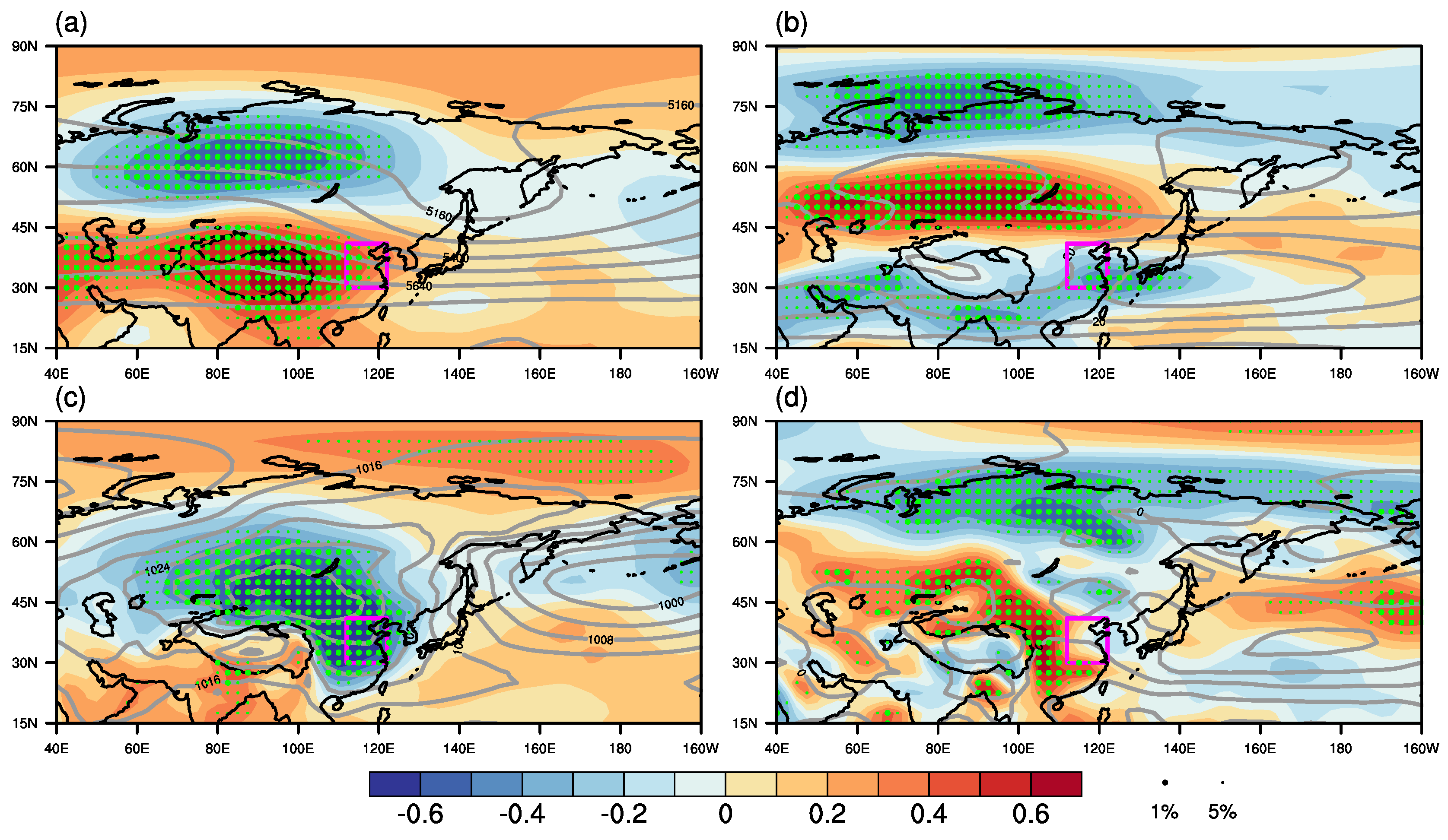
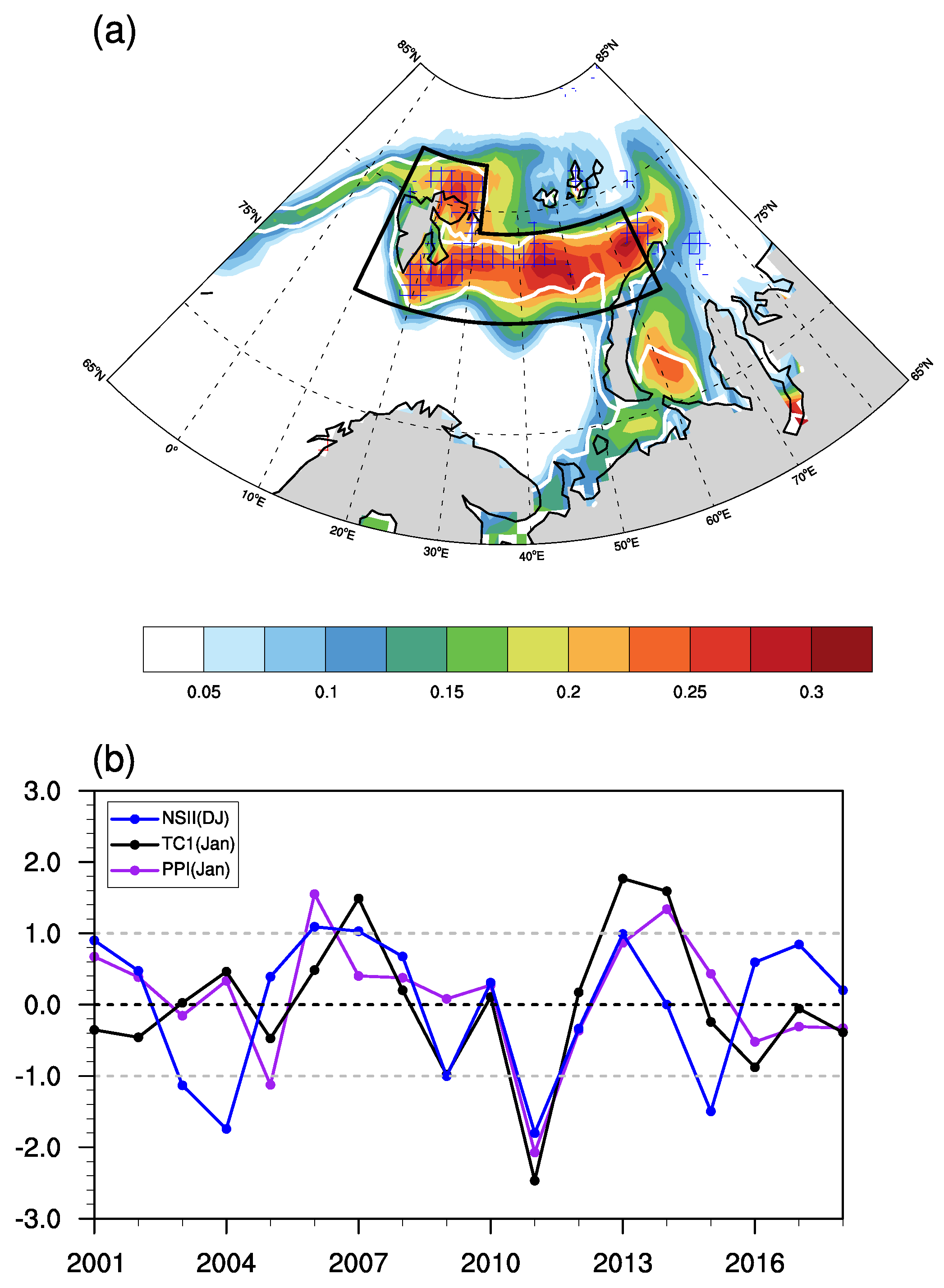
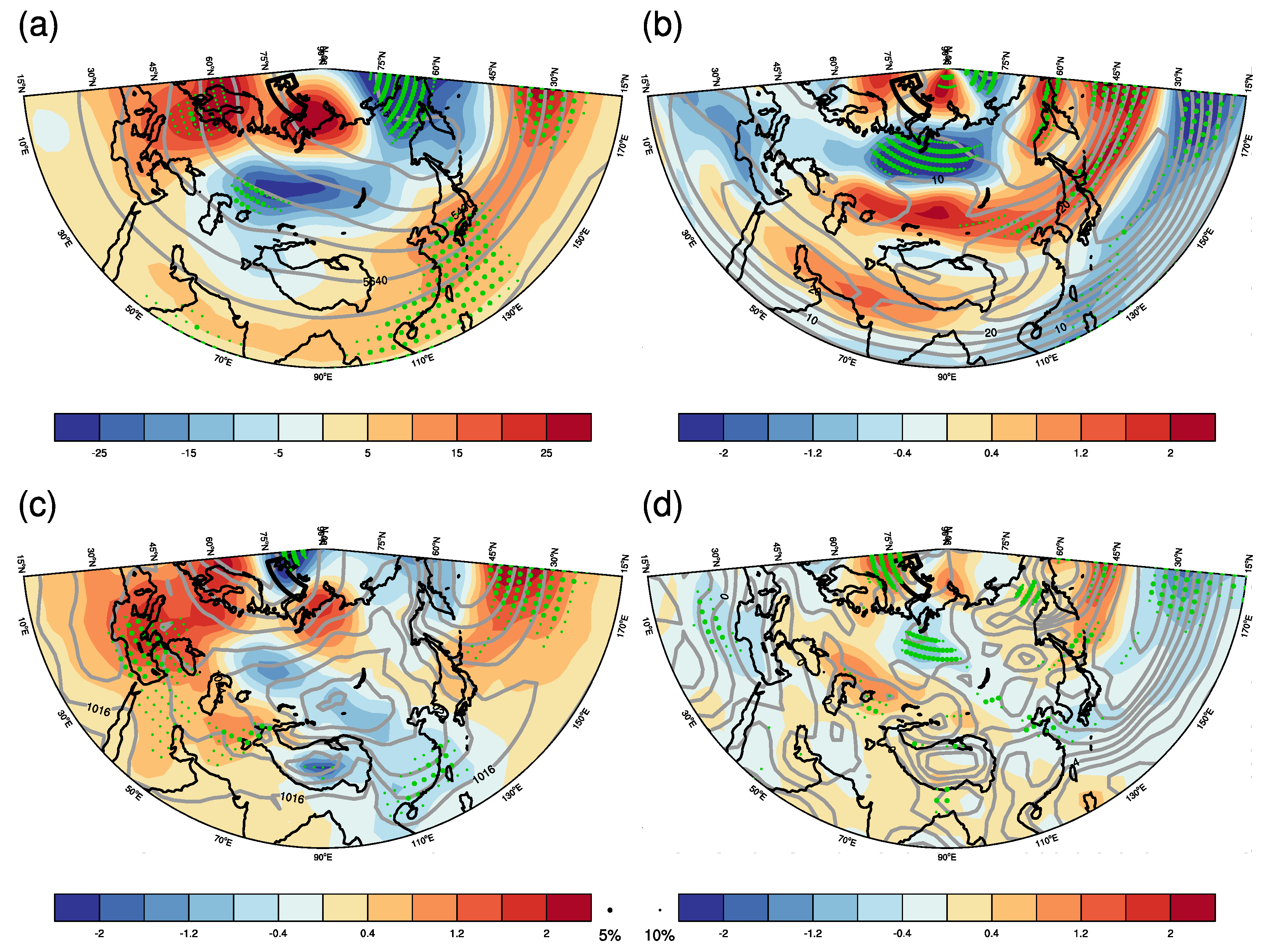
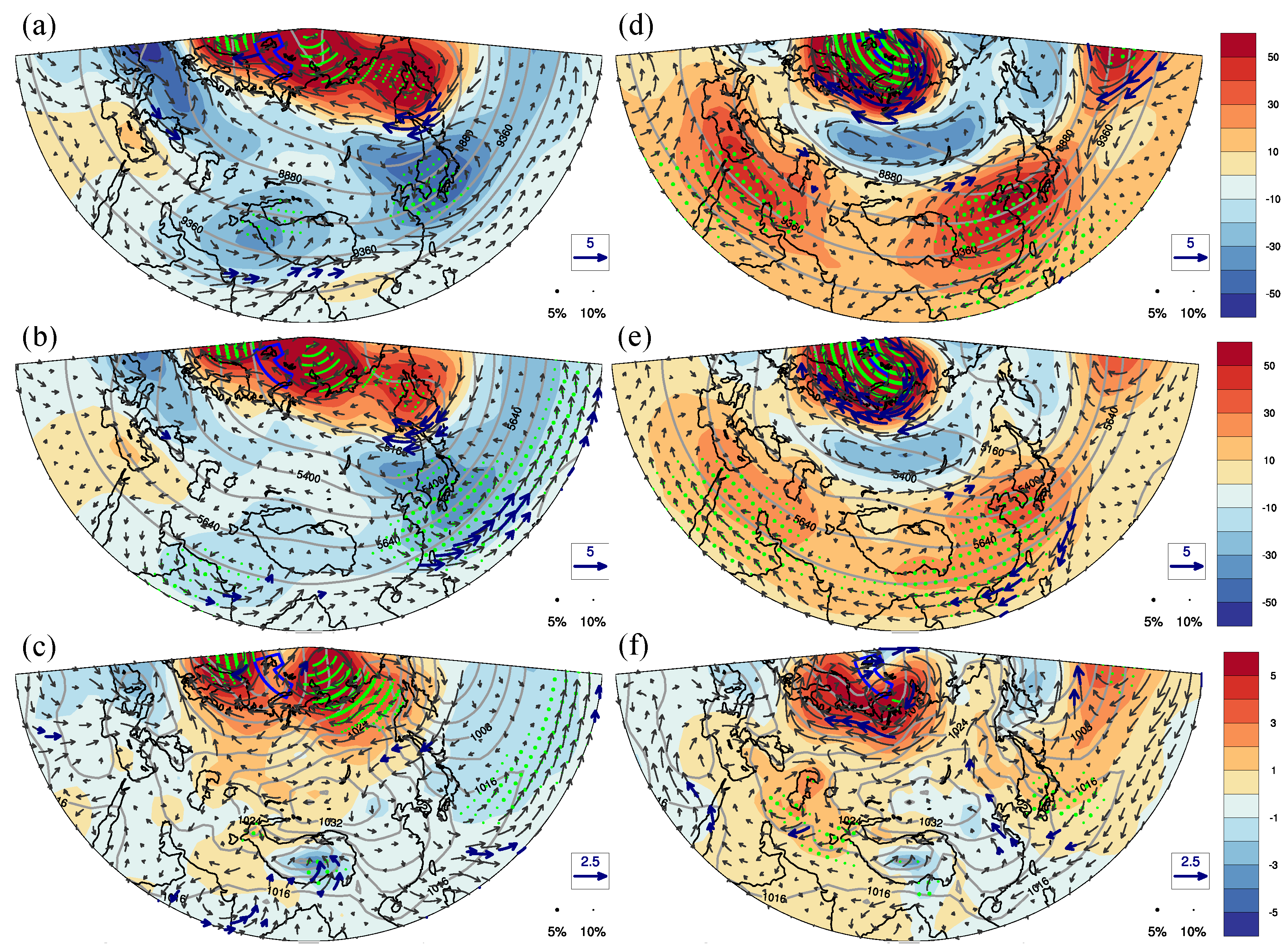
3.3. Possible Impacts of Arctic Sea Ice on PM₁₀ Variability in Korean Peninsula

In Section 3.2, we confirmed that the relative intensification of zonal wind in the north of the Korean peninsula and the relative weakening of the Siberia high and Aleutian low could provide a favorable condition for high concentrations of PM₁₀ in Korea. Therefore, we analyzed the relationship with sea ice concentration Arctic regions in order to investigate the cause of the favorable atmospheric condition that leads to high PM₁₀ pollution in Korea.

Interestingly, TC1 in South Korea is negatively correlated with December-January (DJ) SIC in the Arctic Ocean, especially in the Barents Sea (Figure 6). Moreover, the large variability in SIC over the Barents Sea can have a significant influence on large-scale circulation in the NH [17,18,19,20,21,22]. In order to determine the relationship of PPI with SIC, NSII was calculated by normalizing the area-averaged value of SIC over the Barents Sea (box area in Figure 6a) and then multiplied by a negative value. In

Table 3. Correlation coefficients of TC1 and PPI of January in South Korea with each month’s NSII (negative sea ice index) and DJ (December-January) ASII (Arctic sea ice index). Superscripts indicate significance at the 95%, 90% confidence levels, respectively. Values in parentheses indicate correlation coefficients with NSII for the hatched area of Figure 6a.

CORR	NSII (December)	NSII (January)	NSII (DJ)	ASII (DJ)
TC1	0.45 * (0.52 **)	0.42 * (0.53 **)	0.44 * (0.52 **)	−0.15
PPI	0.35 (0.39)	0.41 * (0.49 **)	0.40 * (0.44 *)	−0.03

* 90%, ** 95% confidence level.

, the NSII is significantly correlated with TC1 (r = 0.44) and PPI (r = 0.40) at 10% and 5% significance levels (values in parentheses), respectively, especially in December and January, indicating that SIC in the preceding winter season can be a good predictor for PM₁₀ concentrations in South Korea. In fact, the up and down pattern of NSII over the Barents Sea coincides with that of PPI, especially in the two extreme cases, i.e., 2011 and 2013. However, it should be noted that total Arctic SIC index (ASII) is not significantly correlated with the TC1 and PPI in South Korea (Table 3). In summary, unlike the ASII, the SIC over the Barents Sea in the DJ season is closely related to the large-scale mode (TC1) of PM₁₀ in January in South Korea. That is, the decrease (increase) in SIC of the Barents Sea is related to the increase (decrease) of PM₁₀ concentrations in South Korea at an inter-annual time scale.

Regression of NSII onto January atmospheric circulation variables was conducted to analyze the effect of SIC over the Barents Sea on PM₁₀ concentrations in South Korea (Figure 7). The regression map shows that the decrease of SIC over the Barents Sea is significantly correlated with a low-pressure anomaly at 500 hPa over the Ural mountain range region and a high-pressure anomaly at 500 hPa over the Korean peninsula. Moreover, the intensification of westerly wind at 500 hPa (Figure 7b) over the regions from the Caspian Sea to Hokkaido, weak Siberian High, and weak Aleutian low (Figure 7c) were related to a decrease of SIC over the Barents Sea. These patterns are similar to the correlation between PPI and atmospheric fields in Figure 4, indicating that the variability of SIC over the Barents Sea can play an important role in modulating the variability of PM₁₀ in South Korea through modulation of atmospheric fields over Eurasia by a teleconnection from the Arctic Ocean to the Korean peninsula via Eurasia, as one of the important forcing factors.

4. Summary and Conclusions

In this study, the possible teleconnection between PM₁₀ concentration in South Korea and Arctic Sea Ice concentration was analyzed at inter-annual time scales using observed PM₁₀ data in South Korea, NCEP R2 data, and NOAA SIC data for 18 years (2001 to 2018). In addition, we used the PPI, defined as the weighted averaging of two ventilation indices, NWSI and ATGI, to represent a potential large-scale ventilation indicator for high PM₁₀ concentrations in South Korea. In this study, we also investigated the Arctic sea ice that induces an atmospheric circulation pattern favorable for PM₁₀ contamination in South Korea.

From the EOF analysis, we found that the first mode (TC1) of PM₁₀ in South Korea, which explained about 27.4% of the total variability, was a large-scale mode representing the same variability in all stations. This indicates that this mode is related to the large-scale circulation favorable for the two ventilation effects. The second mode, which explained about 16.1% of the total variability, is a linearly decreasing trend mode, and it implies that this reduction is in accordance with the major reduction policy established by the Korean government to improve the atmospheric environment [9]. We also analyzed the relationship between the large-scale mode TC1 in South Korea and the two ventilation indices.

The results show that PM₁₀ concentrations in South Korea are more dominantly influenced by the horizontal ventilation effect than the vertical atmospheric stability effect. However, Zou et al. [7] found that PM₁₀ over the ECP region was equally affected by the two ventilation effects. This difference may be related to geographic characteristics, i.e., basin type in the ECP region, and ocean type in South Korea surrounded by sea. For basin type, atmospheric stability can be as important as wind speed to ventilate air out, while for ocean type, wind speed is more effective than atmospheric stability [9,23]. The PPI in South Korea is highly correlated to TC1 with a correlation coefficient of 0.75, indicating that it is a good measure for high PM₁₀ in South Korea at inter-annual time scales. However, this relation is even stronger in the ECP than that in South Korea, indicating that the PPI in the ECP region is a more effective measure than it is in South Korea.

We also investigated the relationship between the PPI and the atmospheric circulation pattern to understand the dynamic link between PM₁₀ and atmospheric circulation. The results show that the increase of PPI in South Korea is related to the anomalous high pressure of 500 hPa over the Korean peninsula, the relative strengthening of zonal winds to the north of the Korean peninsula, and the weakening of the northerly flow to the Korean peninsula. The relative weakening of high pressure over the Ural mountain range region, along with the anomalous high pressure over the Korean peninsula, are especially responsible for relatively strengthening the jet stream to the north of the Korean peninsula, blocking northerly flow to the south and resulting in high PM₁₀ concentrations over the Korean peninsula through the weakening of horizontal ventilation. Using the NSII defined by area-averaged values of the SIC over the Barents Sea during the DJ season, we also investigated the possible impact of Arctic Sea Ice concentration on the PM₁₀ in South Korea during the month of January. The results show that the NSII is positively correlated with PM₁₀ in South Korea with a significance level of 5%, indicating that the SIC decrease over the Barents Sea induced a favorable atmospheric circulation pattern in the northern hemisphere to increase PM₁₀ concentration in South Korea. The regression pattern of the NSII with atmospheric circulation fields confirms that the decrease in SIC over the Barents Sea induces weakening of high pressure over the Ural mountain range region and an anomalous high-pressure anomaly at 500 hPa over the Korean peninsula in January. This teleconnection pattern is consistent with the intensification of the zonal wind to the north of the Korean peninsula, weakening of east-west pressure gradient over the Korean peninsula, and thereby weaker northerly flow than normal, resulting in warming anomaly and high PM₁₀ anomaly over the Korean peninsula. In conclusion, the Sea Ice loss over Barents Sea in the preceding DJ season may increase January PM₁₀ concentration in South Korea.

It should be noted that this conclusion is different from that of Mori et al. [18,19]. Thus, a synthetic analysis was conducted for two periods (Figure 8) in order to explain why this result is different from Mori et al. [18]. The September Barents Sea (BS) SIC reduction resulted in favorable atmospheric conditions that could lead to cold Eurasia and strong Siberian high pressures, reducing the concentration of contamination in January. However, a decrease in DJ BS SIC during the same period would produce favorable conditions that would increase the southerly winds and increase the pollution concentration in January. This means that the results may vary depending on the lead month. In this study, similar synthetic analysis was also performed on the Barents and Kara Sea (BKS) SIC instead of the BS SIC (not shown). The results show that the effects of the September BKS SIC and DJ BKS SIC decrease on the atmospheric circulation over Eurasia in January are different. These results indicate that the effect of Arctic SIC on the January atmospheric circulation over Eurasia may vary depending on the lead month and target SIC region.

It should be noted that there are limitations in this study. First, the total period of observation is only 18 years—from 2001 to 2018. Even though the observation period is short, it has sufficient duration to examine inter-annual variabilities. However, it is necessary to obtain more accumulated long-term observations in the future and examine the observational evidence revealed in this study more closely. Second, even though the size of the Barents Sea is not large in the Arctic, the variability of SIC is large, especially in December and January (Figure 6a). The large variability over the Barents Sea forces the atmosphere by modulating turbulent heat fluxes and the radiation budget. Previous studies have shown that the large variability in SIC over the Barents and Kara Sea can have a significant influence on large-scale circulation in the NH [17,18,19,20,21,22]. Third, the SIC variability in the Barents Sea and PM₁₀ variability in South Korea can be driven by the same weather variability; for example, Arctic Oscillation (AO) or Warm Arctic Cold Eurasia (WACE) patterns. The possibility is still open. Further study is needed to understand the mechanism between SIC variability over the Barents Sea and its influence on atmospheric circulation change over Eurasia using climate model experiments and in-depth analysis.

In this study, we focused on the relationship between the SIC over the Barents Sea and PM₁₀ in South Korea based on statistical analysis. Thus, we still need a climate modelling sensitivity study to clarify the pathway of teleconnection from the Arctic Ocean to the Korean peninsula at various time scales, including the climate change time scale. Although there are some limitations, this study provides valuable information for seasonal predictions of PM₁₀ in South Korea.

References

1. Cai, W.; Li, K.; Liao, H.; Wang, H.; Wu, L. Weather conditions conducive to Beijing severe haze more frequent under climate change. Nat. Clim. Chang. 2017, 7, 257–262. [Google Scholar] [CrossRef]
2. Chen, H.; Wang, H. Haze Days in North China and the associated atmospheric circulations based on daily visibility data from 1960 to 2012. J. Geophys. Res. Atmos. 2015, 120, 5895–5909. [Google Scholar] [CrossRef]
3. Lee, H.J.; Jeong, Y.M.; Kim, S.-T.; Lee, W.-S. Atmospheric Circulation Patterns Associated with Particulate Matter over South Korea and Their Future Projection. J. Clim. Chang. Res. 2018, 9, 423–433. [Google Scholar] [CrossRef]
4. Niu, F.; Li, Z.; Li, C.; Lee, K.H.; Wang, M. Increase of wintertime fog in China: Potential impacts of weakening of the Eastern Asian monsoon circulation and increasing aerosol loading. J. Geophys. Res. Atmos. 2010, 115, 1–12. [Google Scholar] [CrossRef]
5. Wang, H.-J.; Chen, H.-P.; Liu, J. Arctic sea ice decline intensified haze pollution in eastern China. Atmos. Ocean. Sci. Lett. 2015, 8, 1–9. [Google Scholar] [CrossRef]
6. Zhao, S.; Feng, T.; Tie, X.; Long, X.; Li, G.; Cao, J.; An, Z. Impact of Climate Change on Siberian High and Wintertime Air Pollution in China in Past Two Decades. Earth Future 2018, 6, 118–133. [Google Scholar] [CrossRef] [Green Version]
7. Zou, Y.; Wang, Y.; Zhang, Y.; Koo, J.H. Arctic sea ice, Eurasia snow, and extreme winter haze in China. Sci. Adv. 2017, 3, 1–9. [Google Scholar] [CrossRef]
8. Chen, C.; Su, M.; Liu, G.; Yang, Z. Evaluation of economic loss from energy-related environmental pollution: A case study of Beijing. Front. Earth Sci. 2013, 7, 320–330. [Google Scholar] [CrossRef]
9. Kim, H.C.; Kim, S.; Kim, B.-U.; Jin, C.-S.; Hong, S.; Park, R.; Stein, A. Recent increase of surface particulate matter concentrations in the Seoul Metropolitan Area, Korea. Sci. Rep. 2017, 7, 4710. [Google Scholar] [CrossRef]
10. Oh, H.R.; Ho, C.H.; Kim, J.; Chen, D.; Lee, S.; Choi, Y.S.; Song, C.K. Long-range transport of air pollutants originating in China: A possible major cause of multi-day high-PM10 episodes during cold season in Seoul, Korea. Atmos. Environ. 2015, 109, 23–30. [Google Scholar] [CrossRef]
11. Oh, H.R.; Ho, C.H.; Park, D.S.R.; Kim, J.; Song, C.K.; Hur, S.K. Possible relationship of weakened Aleutian low with air quality improvement in Seoul, South Korea. J. Appl. Meteorol. Climatol. 2018, 57, 2363–2373. [Google Scholar] [CrossRef]
12. Kim, Y.P. Air pollution in Seoul caused by aerosols. J. Korean Soc. Atmos. Environ. 2006, 22, 535–553. [Google Scholar]
13. Lee, S.; Ho, C.H.; Lee, Y.G.; Choi, H.J.; Song, C.K. Influence of transboundary air pollutants from China on the high-PM10episode in Seoul, Korea for the period 16–20 October 2008. Atmos. Environ. 2013, 77, 430–439. [Google Scholar] [CrossRef]
14. Lee, S.; Ho, C.H.; Choi, Y.S. High-PM10concentration episodes in Seoul, Korea: Background sources and related meteorological conditions. Atmos. Environ. 2011, 45, 7240–7247. [Google Scholar] [CrossRef]
15. Wie, J.; Moon, B.K. ENSO-related PM10 variability on the Korean Peninsula. Atmos. Environ. 2017, 167, 426–433. [Google Scholar] [CrossRef]
16. Shen, L.J.; Jacob, D.J.; Mickley, L.; Wang, Y.; Zhang, Q. Insignificant effect of climate change on winter haze pollution in Beijing. Atmos. Chem. Phys. 2018, 18, 17489–17496. [Google Scholar] [CrossRef] [Green Version]
17. Huang, X.-T.; Diao, Y.-N.; Luo, D.-H. Amplified winter Arctic tropospheric warming and its link to atmospheric circulation changes. Atmos. Ocean. Sci. Lett. 2017, 2834, 1–11. [Google Scholar] [CrossRef]
18. Mori, M.; Watanabe, M.; Shiogama, H.; Inoue, J.; Kimoto, M. Robust Arctic sea-ice influence on the frequent Eurasian cold winters in past decades. Nat. Geosci. 2014, 7, 869–873. [Google Scholar] [CrossRef]
19. Mori, M.; Kosaka, Y.; Watanabe, M.; Nakamura, H.; Kimoto, M. A reconciled estimate of the influence of Arctic sea-ice loss on recent Eurasian cooling. Nat. Clim. Chang. 2019, 9, 123–129. [Google Scholar] [CrossRef]
20. Kim, H.C.; Kim, S.; Son, S.-W.; Lee, P.; Jin, C.-S.; Kim, E.; Stein, A. Synoptic perspectives on pollutant transport patterns observed by satellites over East Asia: Case studies with a conceptual model. Atmos. Chem. Phys. Discuss. 2016. [Google Scholar] [CrossRef]
21. Kim, B.M.; Son, S.W.; Min, S.K.; Jeong, J.H.; Kim, S.J.; Zhang, X.; Yoon, J.H. Weakening of the stratospheric polar vortex by Arctic sea-ice loss. Nat. Commun. 2014, 5, 1–8. [Google Scholar] [CrossRef] [PubMed]
22. Screen, J.A. Simulated atmospheric response to regional and pan-arctic sea ice loss. J. Clim. 2017, 30, 3945–3962. [Google Scholar] [CrossRef]
23. Zhang, Z.; Xu, X.; Qiao, L.; Gong, D.; Kim, S.-J.; Wang, Y.; Mao, R. Numerical simulations of the effects of regional topography on haze pollution in Beijing. Sci. Rep. 2018, 8, 5504. [Google Scholar] [CrossRef] [PubMed]
Figure 1. Spatial distribution of (a) climatological mean, (b) standard deviation, and (c) time-series of PM10 concentrations in January over 18 years (2001 to 2018) in South Korea. Black, red, orange, and blue lines indicate all stations in South Korea, Seoul, Urban, and the Gosan background stations, respectively (units: µg/m3). Black, red, and blue dash lines indicate trend lines at all stations in South Korea, Seoul, and background stations, respectively. Grey dot-dash line indicates the mean of all stations in South Korea.
Atmosphere 10 00619 g001
Figure 2. (a) Spatial pattern of the first EOF (Empirical orthogonal function) mode of PM10 concentrations in January in South Korea and (b) its corresponding principal component time-series (unitless). The EOF first mode explains 27.4% of the total variance. The linear trend has been removed.
Atmosphere 10 00619 g002
Figure 3. Time-series of TC1 (time coefficient of the first mode, solid, black), ATGI (air temperature gradient index, dotted, orange), NWSI (negative wind speed index, dotted, blue), and PPI (pollution potential index, solid, purple) in January for 40 years from 1979 to 2018 in (a) South Korea and (b) the ECP (East China Plain) region of China (unitless). The grey line indicates one standard deviation.
Atmosphere 10 00619 g003
Figure 4. Correlation map between PPI in South Korea and atmospheric circulations in the northern hemisphere for (a) geopotential height at 500 hPa and (c) sea level pressure; (b) and (d) is zonal wind at 500 hPa and 1000 hPa, respectively. The grey solid line is the climatological mean for 40 years (1979 to 2018). Two circles indicate significance at the 99%, 95% confidence levels, respectively.
Atmosphere 10 00619 g004
Figure 5. Correlation map between PPI in the ECP region and atmospheric circulations in the northern hemisphere for (a) geopotential height at 500 hPa and (c) sea level pressure; (b) and (d) is zonal wind at 500 hPa and 1000 hPa, respectively. The grey solid line is the climatological mean for 40 years (1979 to 2018). Two circles indicate significance at the 99%, 95% confidence levels, respectively.
Atmosphere 10 00619 g005
Figure 6. (a) Correlation maps between TC1 and arctic sea-ice concentrations. Shading indicates standard deviation, and the white line is the climatological mean at 0.15 and 0.70. Hatched indicates positive and negative correlations with significance at the 80% confidence level. (b) Time-series of the NSII (negative sea ice index) in the DJ (December-January) season (blue line), TC1 (black line), and PPI (purple line) in January in South Korea (unitless).
Atmosphere 10 00619 g006
Figure 7. Regression patterns between DJ season’s NSII (shown in Figure 6b) and atmospheric circulations in the northern hemisphere for (a) geopotential height at 500 hPa (m) and (c) sea level pressure (hPa); (b) and (d) is the zonal wind at 500 hPa and 1000 hPa, respectively (m/s). The grey solid line is climatological mean for 18 years (2001 to 2018). Two circles indicate significance at the 95% and 90% confidence levels, respectively.
Atmosphere 10 00619 g007
Figure 8. Composite difference between 10 low SIC years and 10 high SIC years over BS in September (left panel; ac) and December-January (right panel; df) for 37 years (1982 to 2018). Shadings indicate geopotential height anomalies at 300 hPa (upper panels; units: m), 500 hPa (middle panels; units: m), and SLP anomalies (lower panels; units: hPa). The grey solid line is climatological mean for 37 years (1982 to 2018). Vector indicates wind anomalies. Two closed circles indicate significance at the 95% and 90% confidence levels, respectively.
Atmosphere 10 00619 g008