An Adaptive Neuro-Fuzzy Propagation Model for LoRaWAN


1
School of Computing, Engineering and Built Environment, Glasgow Caledonian University, Glasgow G4 0BA, UK
2
School of Engineering and Built Environment, Nathan campus, Griffith University, 170 Kessels Road, Brisbane, QLD 4111, Australia
*
Author to whom correspondence should be addressed.
Appl. Syst. Innov. 2019, 2(1), 10; https://doi.org/10.3390/asi2010010
Submission received: 12 November 2018
/
Revised: 14 February 2019
/
Accepted: 13 March 2019
/
Published: 18 March 2019
(This article belongs to the Special Issue Fuzzy Decision Making and Soft Computing Applications)
Abstract
:This article proposes an adaptive-network-based fuzzy inference system (ANFIS) model for accurate estimation of signal propagation using LoRaWAN. By using ANFIS, the basic knowledge of propagation is embedded into the proposed model. This reduces the training complexity of artificial neural network (ANN)-based models. Therefore, the size of the training dataset is reduced by 70% compared to an ANN model. The proposed model consists of an efficient clustering method to identify the optimum number of the fuzzy nodes to avoid overfitting, and a hybrid training algorithm to train and optimize the ANFIS parameters. Finally, the proposed model is benchmarked with extensive practical data, where superior accuracy is achieved compared to deterministic models, and better generalization is attained compared to ANN models. The proposed model outperforms the nondeterministic models in terms of accuracy, has the flexibility to account for new modeling parameters, is easier to use as it does not require a model for propagation environment, is resistant to data collection inaccuracies and uncertain environmental information, has excellent generalization capability, and features a knowledge-based implementation that alleviates the training process. This work will facilitate network planning and propagation prediction in complex scenarios.
1. Introduction
In recent years, the exponentially increasing number of wireless devices has made the maintenance and efficient planning of wireless networks crucial. Therefore, it is essential to gain a better understanding of propagation and be able to readily predict it in various scenarios. The area of radio propagation has been studied over many decades, during which the physics of the electromagnetic wave and its propagation has been unchanged. Hence, the same free space path loss (FSPL) formula holds to this date. However, telecommunication devices, network requirements and the propagation environment have undergone many developments. Perhaps, adapting to these rapid changes and lack of efficiency and generalization in current models has been the main research incentive in this field. It is clear that establishing an adaptive, efficient and accurate modeling of modern wireless technologies, that is, LoRaWAN, is of great importance. The main contributions of this paper are:
- (a)
- A novel method of propagation modeling is proposed by using an adaptive-network-based fuzzy inference system (ANFIS). This knowledge-based system enables an adaptive model that is capable of incorporating new modeling parameters, depending on the wireless technology, propagation environment and an expert’s knowledge.
- (b)
- A robust method of determining the network size is used to avoid overfitting.
- (c)
- Results from the models are critically analyzed with real-world measurements using a relatively new wireless technology.
This novel implementation has several advantages, however, for the purpose of comparison, firstly, a brief review of current models would be required. The rest of the paper is organized as follows: Section 2 provides a critical review of the conventional propagation models. Section 3 explains the implementation details and advantages of the proposed model. In Section 4, the results of the practical and comparative analysis are demonstrated, and Section 5 provides the findings of this research along with final conclusions.
2. Brief Review of Common Models
There are numerous practical propagation reports and models for various scenarios, such as indoor, outdoor, urban, sea, foliage, undergrounds and even tunnels. Reviewing all of these models would be out of the scope of this research. Instead, only some of the most influential and well-established models, based on the appearance in published literatures, are reviewed. A more comprehensive review of the propagation models is provided in [1].
2.1. Okumura and Hata Models
Okumura’s signal propagation investigation has been a cornerstone in this field. Okumura’s model [2] was built upon a practical data collection in Tokyo, Japan, within the frequency range of 150–2000 MHz. In his model, the path loss estimation depends on the FSPL, antenna gain factor, propagation gains due to mobile/base-station antennae heights and collective correction gain. The latter, collective correction gain, is to compensate for the type of environment, average slope of terrain and finally land/sea parameters. This model is somewhat a more comprehensive version of the log-distance model. Like other nondeterministic methods, Okumura’s model lacks the higher accuracy of deterministic models. In addition, independent parameters of this model, such as frequency, and mobile and base station antenna heights, were limited in their range. Okumura’s findings then became the basis of the Hata model [3], also known as the Okumura–Hata model. This model introduces many more independent parameters, such as reflection, diffraction and scattering factors. It suggests new correction factors for suburban and rural environments, and extends the range of the parameters of Okumura’s model, such as mobile and base station antenna heights. The International Telecommunication Union (ITU) model [4] was inspired by Okumura’s and Hata’s models.
2.2. Walfisch, Ikegami and Ray Tracing Models
Walfisch and Bertoni [5] proposed a semi-deterministic model that added new modeling parameters into Okumura’s model. These parameters were added to account for the multiple-screen diffraction, caused by the buildings and structures. Ikegami et al. [6] took a new approach by using a simplified ray-tracing method. They assumed multiple-reflected/diffracted waves were highly attenuated and, therefore, only accounted for first-reflected/diffracted rays. The other compromise of this deterministic model was perhaps due to the limited computational power, since the reflection/diffraction losses were approximated with constant values. There are several 2D and 3D ray-tracing algorithms, based on the geometrical optics, uniform theory of diffraction and geometrical theory of diffraction. These models have complemented Ikegami’s efforts. For instance, it is possible to consider two- and three-fold reflections/diffraction, and reflection/diffraction factors depend on the angle of incidence and permittivity of materials. Further detailed summaries of these models with their implementations are provided in [7,8,9,10]. Nevertheless, there are the following drawbacks to these deterministic models:
- (a)
- (b)
- Computational complexity of the ray tracing is extremely cumbersome even in a relatively small indoor environment and the accuracy of the model depends on the accuracy of the structural model [12]. Therefore, it is not really a practical solution for outdoor large-scale modeling.
- (c)
These drawbacks are even more aggravated when the radio frequency is increased.
2.3. COST Action 231 Model
The European Cooperation in Science and Technology (COST) Action 231 [15] proposed a new propagation model, plus an extension to the previous Hata model. The COST–Hata PCS Extension simply extended the original Hata model to be applicable to frequencies up to 2 GHz. The COST–Walfisch–Ikegami (COST W.I.) model, however, provided a revised version of the Walfisch and Ikegami models, except that it does not require a 2/3D model of the environment. Eliminating this requirement is perhaps the main advantage of COST W.I., making it the most commonly used outdoor model. COST W.I. has been recommended by ITU and the European Telecommunication Standards Institute (ETSI) [16]. The model still requires the height of the buildings, width of the streets and some other environmental information, and therefore, it is not a fully deterministic model [17]. Although COST W.I. (or models similar to it) may seem to be an acceptable compromise between accuracy and computational complexity, it is rather a granulated set of formulas which has the following disadvantages:
- (a)
- Some of the model parameters lack clear physical or practical interpretation. For instance, the angle of arrival of the beam relative to the axis of the road (ϕ) and road width () are vague at a crossroad, junction, riverside or a wide highway with partial line of sight (LoS), and undefined where there is no road. These conditions and many others that may occur are not considered in the COST W.I. formulas.
- (b)
- The constant factors that control the loss due to intensity of multiscreen diffraction are discontinuous, resulting in abrupt changes in the result. For instance, scatter loss (ϕ) has sharp transitions as it has been approximated with only three piecewise linear functions. Therefore, a small variation in ϕ can affect the estimation drastically.
- (c)
- There are several different permutations and possibilities to calculate the total path loss. The model first differentiates between LoS and NLoS (non-line of sight) conditions. Next, there are two ways of deriving the path loss depending on the . The NLoS has been further subdivided to scatter and diffraction losses. Next, there are three different conditional statements to calculate the scatter loss depending on the ϕ. Finally, there are another 11 further subdivisions (depending on BS and MS heights and environment type) to calculate the multiscreen diffraction loss. However, in reality, even differentiating between LoS and NLoS is difficult, resulting in the creation of near-LoS or partial-LoS conditions [18].
2.4. Hybrid and Artificial Neural Network-Based Models
The next generation of the propagation models relies on artificial neural networks (ANNs). These models are based on the training of an ANN with empirically collected data. Usually this involves training the ANN from scratch, where the ANN has to learn to derive the very basic mechanisms of radio propagation. For instance, the ANN even needs to learn the trivial fact that increasing the link distance has a negative impact on the signal strength. It is the ANN’s responsibility to learn the FSPL from the distance and frequency of transmission or understand the attenuating impact of obstacles on the LoS. A review of the ANN-based models is provided in [19]. The drawbacks of this approach include:
- (a)
- the time-consuming and exhaustive data collection process that is required for the training of ANNs. As an instance, in [20], authors collected 600,000 data samples in a relatively small indoor environment and trained the network for several hours. Not only is such data collection in a small environment tedious but it also defeats the purpose of estimation [19].
- (b)
To address these challenges, a hybrid model for a simple indoor environment was proposed [19]. The model comprised an optimized multiwall model (MWM), whose estimations were monitored by an ANN. Therefore, the ANN only had to learn and compensate the deficiencies of the MWM. This strategy drastically reduced the required training data samples and improved the accuracy of the estimation. A relatively similar strategy was employed in [23,24] using the COST W.I. There are, however, two drawbacks of the latter implementations:
- (a)
- Selecting an appropriate and flexible model for a complicated outdoor environment where many propagation mechanisms are involved is challenging. In fact, Hosseinzadeh et al. [19] had to slightly adjust the MWM according to their requirement.
- (b)
- Conventional models are not tailored or flexible enough to represent the novel characteristics of communication devices. For instance, to the best of our knowledge, there is no propagation model that takes the spreading factor () of a chirp spread spectrum modulation (CSS) [25] into consideration. Theoretically, a higher provides a higher processing gain and, therefore, improves the range. Including such technology-dependent parameters not only increases the modeling accuracy and makes the models more compatible with new devices, but it also helps modeling the signal propagation of the whole system rather than estimation of the path loss only.
3. Proposed Model Description
To address the explained shortfalls and challenges, an adaptive neuro-fuzzy model is proposed. This allows the user to initiate the system with incorporated linguistic knowledge of propagation and then train the system further to achieve a higher accuracy. Next, the essential fuzzy/linguistic input–output parameters of a propagation model are identified. Furthermore, to avoid overfitting and achieve a better generalization, an efficient clustering method to determine the optimum size of the nodes is used. Finally, the system is trained with a hybrid algorithm that tunes the input and output parameters of the fuzzy system. This section explains the implementation details.
3.1. Adaptive Neuro-Fuzzy Inference System for Propagation Estimation
Fuzzy systems are universal approximators of nonlinear dynamic systems [26,27]. The idea of fuzzy sets, fuzzy logics and consequently fuzzy inference systems was first proposed by Zadeh [28]. As stated by Zadeh, fuzzy systems “provide an approximate and yet effective means of describing the behavior of systems which are too complex or too ill-defined to admit of precise mathematical analysis” [29]. The humanistic nature of the fuzzy systems allows us to define a complex system with fuzzy/linguistic variables using a human-like reasoning instead of using conventional mathematical tools or precise quantitative analysis. Fuzzy systems provide some degree of resistance to handle vague, ambiguous, imprecise, noisy, missing and uncertain information [30,31,32,33]. This should provide the level of flexibility required to deal with data that is hard or rather impossible to accurately infuse into the model, such as the and . This resistance also relaxes the inevitable inaccuracies in data collection. This is mainly due to the fuzzification of continuous variables. The fuzzification process transforms the crisp value of the inputs () to degrees of membership using a membership function (). Next, these membership functions are tuned using the gradient-descent algorithm to optimize the output. Changes in the are therefore affecting the degrees of membership of the inputs ().
The proposed ANFIS architecture comprises first-order Tagaki-Sugeno (T-S)-type fuzzy systems [34], where the output membership functions are first-order polynomials. Therefore, a hybrid training allows a linear least-squares estimation to be used for the identification of the consequent parameters, and a gradient descent optimization is used to identify the premise parameters [30,35]. Compared to most neural networks, ANFIS also has fewer parameters, many of which can be tuned with linear least-squares. These features give ANFIS the advantage of fast training and computational speed; furthermore, since there are fewer tunable parameters, the pitfall of overfitting the data would be avoided [36].
The T-S fuzzy implication (if–then rule) is analogous to that of defining a nonlinear input–output mapping. The process can be interpreted as the decomposition of a system into a finite number of subsystems and then approximating each subsystem. The output of the T-S is determined by the aggregation of the implications. Considering a number of implications , with antecedents (premise) and consequences , implication th is of the format of Equation (1),
where is the input vector (premise variable), contains the membership functions of the th input, is the consequence parameters vector, and is the normalized firing strength, or truth value, of the implication .
3.2. Model Input
A relatively similar set of inputs that are defined in the COST231 model was considered, however, three additional inputs were added based on our knowledge of propagation and common sense. In addition, three of the COST231 inputs (base station height, mobile station height and their height difference) were combined into one. Many of these modeling inputs were acquired from Google maps to further facilitate the modeling. The only output of the system is the received signal strength indicator (). These inputs are explained as follows:
- (a)
- spreading factors () of LoRa’s CSS modulation (7 12);
- (b)
- height difference () between the base station () and mobile station (), where is the altitude of earth at the location of measurement;
- (c)
- free space path loss () to include the effect of frequency, is the wavelength of transmission and is the LoS distance (regardless of obstruction) between transceivers;
- (d)
- clutter ratio () in the LoS, total number of buildings and structures in LoS, regardless of their heights;
- (e)
- acute angle between the LoS and the axis of the road ();
- (f)
- relative width of the street ();
- (g)
- defined as the length of LoS that is on the water divided by the ;
where and are acquired from Google map images and, therefore, may have some inaccuracies. For certain scenarios, some of these parameters may not be very important, or may not exist, and therefore, would not apply at all.
3.3. Model Identification
Various membership functions including triangular, trapezoidal and sigmoidal were examined for the fuzzification; however, a normalized Gaussian membership function, with the general form of Equation (2), yielded the best result, where is the standard deviation and determines the spread of , and is the mean, which determines the center of the .
Two approaches were considered for the identification of the premise structure. The first approach was to define fuzzy if–then rules using all the possible permutations of all or some of the fuzzified inputs. For instance, using common sense knowledge of propagation one could define the following implication:
- “If is short and is high and is clear then is good.”
This states that “if the transmission was done over a short distance, with a high spreading factor, and the LoS was relatively clear of clutter, then reception should be good, regardless of other input parameters”. However, this approach can be prone to combinatorial explosion of rules, especially for complex systems. Considering that there was a total of seven inputs, each with two membership functions, then the total number of rules is .
The second approach was to use a clustering method [36]. A subtractive clustering [37] was chosen for the identification of the rules, since subtractive clustering does not require an initial estimate of the center or the number of clusters [38]. Other clustering algorithms could be used, where eventually, each cluster center forms a fuzzy rule.
A first-order T-S model was selected, as it provided a higher accuracy compared to zero-order T-S. Hence, output membership functions were of the form in Equation (1), where the output linear functions () were identified by linear least-squares optimization.
4. Analysis and Results
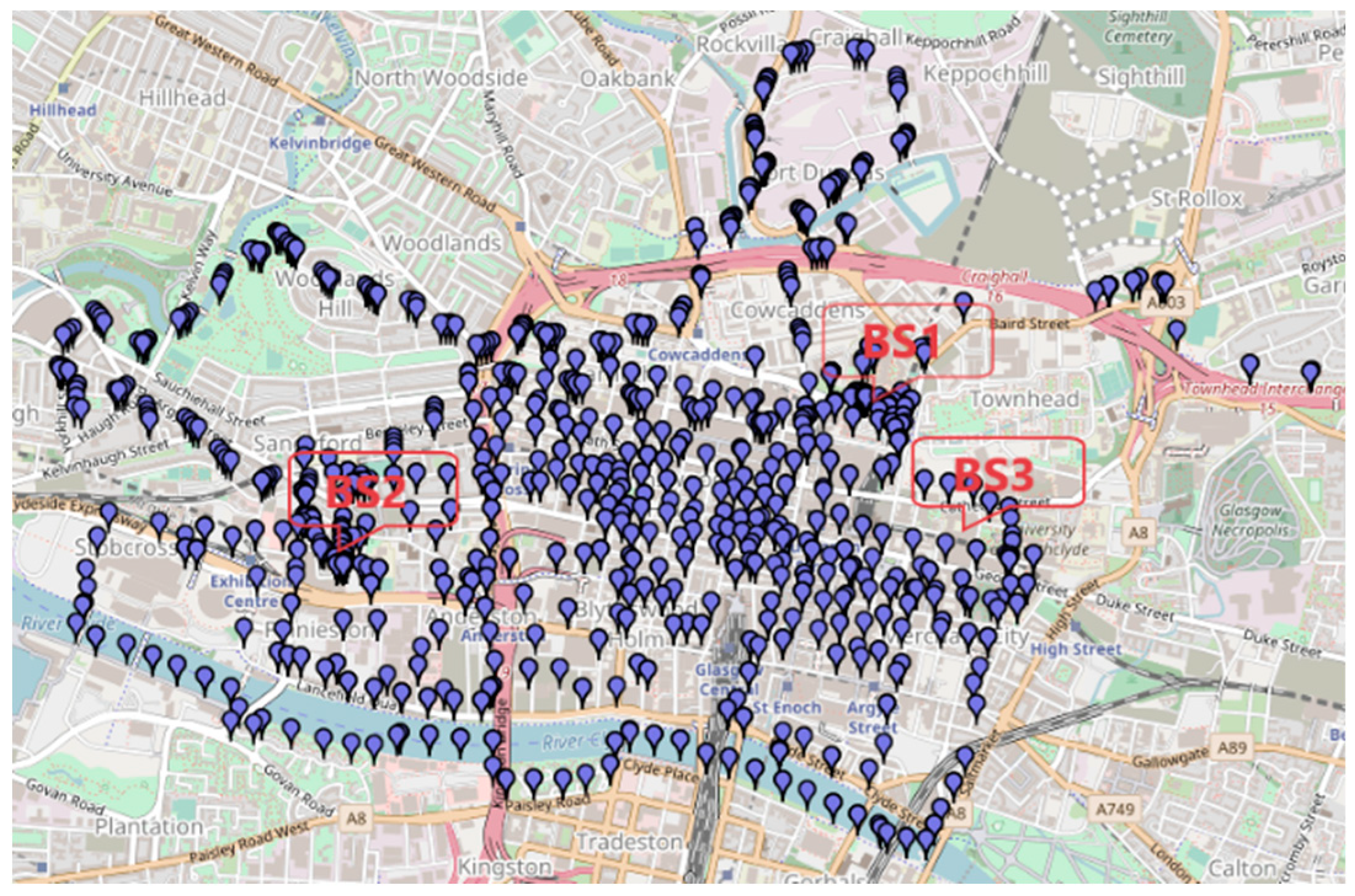
About 5000 data samples were collected over a relatively large area (4.25 km × 2.7 km) in the commercial area of Glasgow, Scotland. Data was collected from three base stations at different locations, with 1931, 1820 and 1256 samples being collected from BS1, BS2 and BS3, respectively. Figure 1 shows the area of the investigation, where some of the measurement locations are pinpointed with markers, and gateways are labeled as BS1, BS2 and BS3. Base stations are equipped with the same antennae, mounted relatively at the same height from the ground. Data was analyzed to provide an insight of the performance of the proposed model.
To check the goodness of fit and benchmarking with other models, the most commonly used measures in the literature were reported, RMSE (root mean square error in dB), (error standard deviation dB) and (mean error dB). Unfortunately, the first two measures depend on the range or scale of data and ignores the error sign. Therefore, to address these issues, the Nash-Sutcliffe efficiency (NSE) coefficient is used as a measure of the goodness of the fit. Having a universal measure of performance benchmarking is especially important, as various wireless technologies have different sensitivities. This difference impacts the dynamic range of measured data and, therefore, its RMSE scale; however, the NSE is less prone to the dynamic range. NSE ranges from −∞ to 1, where 1 would indicate a perfect match between the model predictions and measurements [39].
In addition, to investigate the model’s generalization capability, instead of training with one BS at a time, data from all the three BSs was used to train and validate the model. For the purpose of comparison, an ANN model was also used to model the propagation. A feedforward ANN was chosen with three hidden layers of size seven, 14 and four neurons for each layer, respectively. The best ANN structure was chosen heuristically after trying ANNs with two to five hidden layers of various neuron sizes. Results in Table 1 demonstrate the average of a 10-fold cross-validation analysis; 90% of data was used for training.
The results of the COST W.I. model are tabulated in Table 2 to make a comparison with other practical investigations conducted in [15].
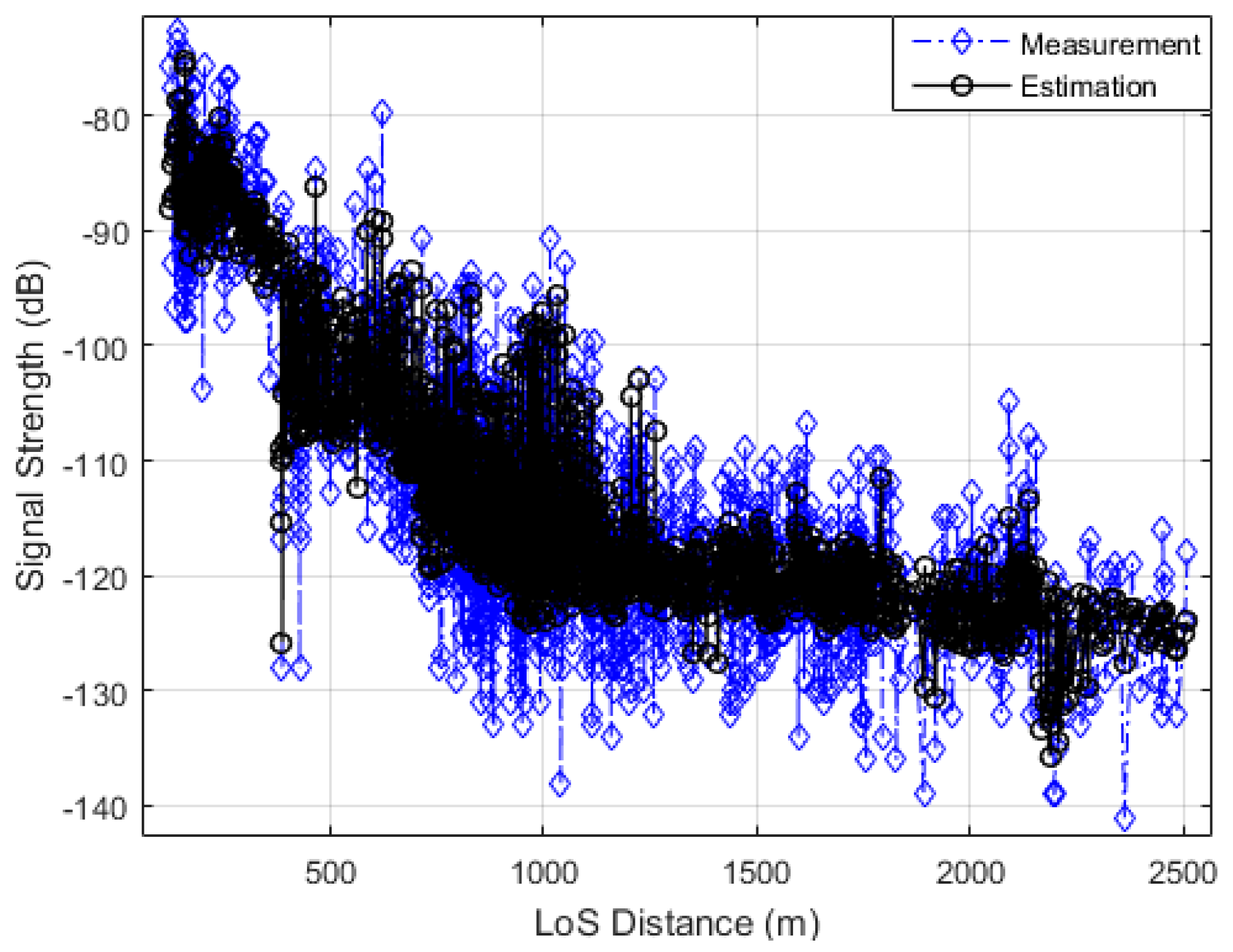
Figure 2 compares the measurements and estimation for BS1, and Figure 3 compares the overall estimation of all base stations with measurements.
A series of models were benchmarked against similar practical measurements in COST Action 231 [15]. In this comparison, 970, 335 and 1031 samples were collected from three different base stations in Munich, Germany. Propagation models were then used to estimate the signal strength only for each individual site. Since the examined models were either deterministic or semi-deterministic, 2D or 3D building layout and building height information were provided to the models in the study conducted by COST, whereas the COST231 in this article only used the collected environmental information that was explained earlier (Section 3.2). In Table 3, only the range of measures (maximum and minimum of and ) of COST performance analysis report are included. A detailed performance of each model can be found in Table 4.5.2 of COST Action 231 Chapter 4 [15]. Unfortunately, other performance metrics such and RMSE, NSE and MAE are not stated in this report. Therefore, the RMSE in Table 3 is extracted for instances with (if then RMSE = ). Table 3 is provided as a measure of overall modelling accuracy that can be achieved given the availability of 2D or 3D environmental information.
To further observe the generalization capability of the ANFSI model, only 20% of the data was used for training. These results are tabulated in Table 4.
5. Discussion and Conclusions
The decomposition of a propagation system into smaller subsystems has been the ultimate goal of the Okumura, Hata and COST models. In fact, the suggestion of the breaking point-distance phenomenon in ITU recommendation P.1411 [40] follows the same idea. These attempts used crisp or Boolean logic to differentiate between a limited set of propagation conditions or scenarios. In contrast to sudden transitions, fuzzy logics make it possible to have smoother transitions, while mitigating the uncertainties within the data. ANFIS further allowed for the implementation of an expert’s knowledge into the system, which addressed part of the challenges of the ANN models.
Comparison of the models used in this investigation indicated that the ANFIS and ANN models resulted in a remarkably better performance in terms of estimation, compared to the COST W.I. model. The ANFIS model resulted in a better performance compared to the ANN model. and NSE were consistently improved by about 1 dB and 10%, respectively. ANFIS was found as a better generalization candidate. In this study, the performance of ANN in Table 1 was almost identical to the ANFIS results in Table 4. This is while the ANN was trained with 90% of the data, whereas ANFIS achieved the same results with only 20% of the data.
Furthermore, two new parameters were added into the model without having to formulate them. was required due to the wireless technology of choice, and was added due to the features of the propagation environment. Inclusion of these parameters in the modeling reduced the RMSE and NSE of the ANFIS model by 0.55 dB and 7%, respectively. These two parameters, however, did not make a significant change to the ANN model results. This might be due to the limited number of measurements (380 samples) that had . This is the most likely reason, given that ANFIS, with a better generalization, could benefit from this parameter.
In this investigation, the proposed ANFIS model was used for outdoor environments. However, it can be easily adopted for indoor propagation as well. This is as simple as providing the impacting propagation parameters for the system and roughly describing their effect using fuzzy linguistic reasoning. For instance, in an indoor environment, the effect of a higher number of walls, windows or doors on LoS can increase the loss.
Author Contributions
S.H. and A.W. conceived and designed and performed the experiments; S.H. analyzed the data; H.L. and K.C. contributed materials/analysis tools; S.H., K.C. and H.L. wrote the paper reported.
Funding
This research received no external funding.
Acknowledgments
The authors would like to thank Glasgow Caledonian University for funding this research. Also, Stream Technologies for facilitating the data collection and measurements, and Innovate UK (KTP).
Conflicts of Interest
The authors declare no conflict of interest.
References
- Sarkar, T.K.; Ji, Z.; Kim, K.; Medouri, A.; Salazar-Palma, M. A survey of various propagation models for mobile communication. IEEE Antennas Propag. Mag. 2003, 45, 51–82. [Google Scholar] [CrossRef]
- Okumura, Y.; Ohmori, E.; Kawano, T.; Fukuda, K. Field strength and its variability in VHF and UHF land-mobile radio service. Rev. Electr. Commun. Lab. 1968, 16, 825–873. [Google Scholar]
- Hata, M. Empirical formula for propagation loss in land mobile radio services. IEEE Trans. Veh. Technol. 1980, 29, 317–325. [Google Scholar] [CrossRef]
- Propagation Data and Prediction Methods for the Planning of Indoor Radio Communication Systems and the Radio Local Area Networks in the Frequency Range 900 MHz to 100 GHz; ITU-R Recommendations Series, P. International Telecommunication Union: Geneva, Switzerland, 2015.
- Walfisch, J.; Bertoni, H.L. A theoretical model of UHF propagation in urban environments. IEEE Trans. Antennas Propag. 1988, 36, 1788–1796. [Google Scholar] [CrossRef]
- Ikegami, F.; Takeuchi, T.; Yoshida, S. Theoretical prediction of mean field strength for urban mobile radio. IEEE Trans. Antennas Propag. 1991, 39, 299–302. [Google Scholar] [CrossRef]
- Hosseinzadeh, S.; Larijani, H.; Curtis, K. An enhanced modified multi wall propagation model. In Proceedings of the Global Internet of Things Summit (GIoTS), Geneva, Switzerland, 6–9 June 2017. [Google Scholar]
- Hosseinzadeh, S. Multi-wall Signal Propagation Model. 2016. Available online: http://www.mathworks.com/matlabcentral/fileexchange/61340-multi-wall--cost231----free-space-signal-propagation-models (accessed on 10 November 2018).
- Hosseinzadeh, S. 3D Ray Tracing For Indoor Radio Propagation. 2017. Available online: https://uk.mathworks.com/matlabcentral/fileexchange/64695-3d-ray-tracing-for-indoor-radio-propagation (accessed on 10 November 2018).
- Hosseinzadeh, S.; Larijani, H.; Curtis, K.; Wixted, A.; Amini, A. Empirical propagation performance evaluation of LoRa for indoor environment. In Proceedings of the 2017 IEEE 15th International Conference on Industrial Informatics (INDIN), Emden, Germany, 24–26 July 2017. [Google Scholar]
- Damosso, E. Digital Mobile Radio towards Future Generation Systems: COST Action 231; European Commission: Luxembourg, Belgium, 1999. [Google Scholar]
- Yuan, D.; Shen, D. Analysis of the Bertoni-Walfisch propagation model for mobile radio. In Proceedings of the 2011 Second International Conference on Mechanic Automation and Control Engineering (MACE), Hohhot, China, 15–17 July 2011. [Google Scholar]
- Qiu, L.; Jiang, D.; Hanlen, L. Neural network prediction of radio propagation. In Proceedings of the 6th Australian Communications Theory Workshop, Brisbane, Australia, 2–4 February 2005. [Google Scholar]
- Teal, P.D.; Kennedy, R.A. Bounds on extrapolation of field knowledge for long-range prediction of mobile signals. IEEE Trans. Wirel. Commun. 2004, 3, 672–676. [Google Scholar] [CrossRef]
- COST, Final Report for COST Action 231; Chapter 4; COST: Luxembourg, Belgium, 1999.
- Correia, L.M. A view of the COST 231-Bertoni-Ikegami model. In Proceedings of the 3rd European Conf. Antennas and Propagation, Berlin, Germany, 23–27 March 2009. [Google Scholar]
- Hamim, S.F.; Jamlos, M.F. An overview of outdoor propagation prediction models. In Proceedings of the 2014 IEEE 2nd International Symposium on Telecommunication Technologies (ISTT), Langkawi, Malaysia, 24–26 November 2014. [Google Scholar]
- Sorrentino, A.; Nunziata, F.; Ferrara, G.; Migliaccio, M. An effective indicator for NLOS, nLOS, LOS propagation channels conditions. In Proceedings of the 2012 6th European Conference on Antennas and Propagation (EUCAP), Prague, Czech Republic, 26–30 March 2012. [Google Scholar]
- Hosseinzadeh, S.; Almoathen, M.; Larijani, H.; Curtis, K. A Neural Network Propagation Model for LoRaWAN and Critical Analysis with Real-World Measurements. Big Data Cogn. Comput. 2017, 1, 7. [Google Scholar] [CrossRef]
- Neskovic, A.; Neskovic, N. Microcell electric field strength prediction model based upon artificial neural networks. AEU-Int. J. Electron. Commun. 2010, 64, 733–738. [Google Scholar] [CrossRef]
- Parsons, J.D. The Mobile Radio Propagation Channel; Wiley & Sons: Chichester, UK, 1992. [Google Scholar]
- Ostlin, E.; Zepernick, H.-J.; Suzuki, H. Macrocell path-loss prediction using artificial neural networks. IEEE Trans. Veh. Technol. 2010, 59, 2735–2747. [Google Scholar] [CrossRef]
- Popescu, I.; Nikitopoulos, D.; Constantinou, P.; Nafornita, I. ANN prediction models for outdoor environment. In Proceedings of the 2006 IEEE 17th International Symposium on Personal, Indoor and Mobile Radio Communications, Helsinki, Finland, 11–14 September 2006. [Google Scholar]
- Gschwendtner, B.E.; Landstorfer, F.M. Adaptive propagation modelling using a hybrid neural network technique. Electron. Lett. 1996, 32, 162–164. [Google Scholar] [CrossRef]
- Semtech Corporation, LoRa™ Modulation Basics. 2015. Available online: https://www.semtech.com/uploads/documents/an1200.22.pdf (accessed on 10 November 2018).
- Castro, J.L. Fuzzy logic controllers are universal approximators. IEEE Trans. Syst. Man Cybern. 1995, 25, 629–635. [Google Scholar] [CrossRef] [Green Version]
- Kosko, B. Fuzzy systems as universal approximators. IEEE Trans. Comput. 1994, 43, 1329–1333. [Google Scholar] [CrossRef]
- Zadeh, L.A. Fuzzy sets. In Fuzzy Sets, Fuzzy Logic, And Fuzzy Systems: Selected Papers by Lotfi A Zadeh; World Scientific: Singapore, 1996; pp. 394–432. [Google Scholar]
- Zadeh, L.A. Fuzzy logic. Computer 1988, 21, 83–93. [Google Scholar] [CrossRef]
- Hosseinzadeh, S. A Fuzzy Inference System for Unsupervised Deblurring of Motion Blur in Electron Beam Calibration. Appl. Syst. Innov. 2018, 1, 48. [Google Scholar] [CrossRef]
- Jang, J.-S.R. ANFIS: Adaptive-network-based fuzzy inference system. IEEE Trans. Syst. Man Cybern. 1993, 23, 665–685. [Google Scholar] [CrossRef]
- Priyono, A.; Ridwan, M.; Alias, A.J.; Atiq, R.; Rahmat, O.K.; Hassan, A.; Ali, M. Generation of fuzzy rules with subtractive clustering. J. Teknol. 2005, 43, 143–153. [Google Scholar] [CrossRef]
- Hosseinzadeh, S. Unsupervised spatial-resolution enhancement of electron beam measurement using deconvolution. Vacuum 2016, 123, 179–186. [Google Scholar] [CrossRef]
- Takagi, T.; Sugeno, M. Fuzzy identification of systems and its applications to modeling and control. IEEE Trans. Syst. Man Cybern. 1985, SMC-15, 116–132. [Google Scholar] [CrossRef]
- De Mingo López, L.F.; Blas, N.G.; Arteta, A. The optimal combination: Grammatical swarm, particle swarm optimization and neural networks. J. Comput. Sci. 2012, 3, 46–55. [Google Scholar] [CrossRef] [Green Version]
- Chiu, S.L. Fuzzy model identification based on cluster estimation. J. Intell. Fuzzy Syst. 1994, 2, 267–278. [Google Scholar]
- Surmann, H.A. Selenschtschikow and others, Automatic generation of fuzzy logic rule bases: Examples I. In Proceedings of the NF2002: First International ICSC Conference on Neuro-Fuzzy Technologies CUBA, Havana, Cuba, 16–19 January 2002. [Google Scholar]
- Yager, R.R.; Filev, D.P. Generation of fuzzy rules by mountain clustering. J. Intell. Fuzzy Syst. 1994, 2, 209–219. [Google Scholar]
- Ritter, A.; Muñoz-Carpena, R. Performance evaluation of hydrological models: Statistical significance for reducing subjectivity in goodness-of-fit assessments. J. Hydrol. 2013, 480, 33–45. [Google Scholar] [CrossRef]
- Propagation Data and Prediction Methods for the Planning of Short-range Outdoor Radio Communication Systems and Radio Local Area Networks in the Frequency Range 300 MHz to 100 GHz; ITU-R Recommendations Series, P. International Telecommunication Union: Geneva, Switzerland, 2017.
Figure 1.
Area of practical investigation 4.25 km × 2.7 km, and base station locations (BS1, BS2, BS3). A few measurement locations are pinpointed with markers.
Figure 1.
Area of practical investigation 4.25 km × 2.7 km, and base station locations (BS1, BS2, BS3). A few measurement locations are pinpointed with markers.

Figure 2.
ANFIS estimations vs practical measurements at BS1.

Figure 3.
ANFIS estimation vs practical measurements at all BSs.


Table 1.
ANFIS and ANN model performance with 10-fold cross-validation.
| ANFIS | |||||
| Base Station | RMSE | MAE | NSE | ||
| BS1 | 5.783 | 5.788 | 0.022 | 4.582 | 0.58 |
| BS2 | 6.631 | 6.621 | 0.050 | 5.196 | 0.56 |
| BS3 | 6.290 | 6.285 | 0.026 | 5.017 | 0.38 |
| BS1,2,3 | 7.060 | 7.056 | 0.014 | 5.495 | 0.48 |
| ANN | |||||
| BS1 | 6. 233 | 6.231 | 0.002 | 4.905 | 0.51 |
| BS2 | 8.249 | 8.257 | −0.103 | 6.457 | 0.44 |
| BS3 | 7.045 | 7.037 | 0.029 | 5.617 | 0.30 |
| BS1,2,3 | 8.128 | 8.127 | 0.167 | 6.388 | 0.38 |
Table 2.
COST W.I. model performance with optimization.
| Base Station | RMSE | MAE | NSE | ||
|---|---|---|---|---|---|
| BS1 | 12.37 | 10.61 | 6.367 | 10.54 | 0.039 |
| BS2 | 18.94 | 14.12 | 12.63 | 16.25 | −0.27 |
| BS3 | 13.33 | 12.46 | 4.752 | 11.04 | −0.30 |
| BS1,2,3 | 18.14 | 12.02 | 13.58 | 15.86 | −0.37 |
Table 3.
Range of standard deviation and mean in COST W.I. measurements [15].
Table 3.
Range of standard deviation and mean in COST W.I. measurements [15].
| RMSE | |||||
|---|---|---|---|---|---|
| min | max | min | max | min | max |
| 6.0 | 21.6 | −0.1 | 21.8 | 7 | 13.8 |
Table 4.
ANFIS model performance with 20% training data.
| Base Station | RMSE | MAE | NSE | ||
|---|---|---|---|---|---|
| BS1 | 6.193 | 6.191 | −0.037 | 4.887 | 0.51 |
| BS2 | 8.035 | 8.014 | −0.017 | 6.233 | 0.46 |
| BS3 | 7.451 | 7.445 | 0.153 | 5.837 | 0.27 |
| BS1,2,3 | 8.0917 | 8.0891 | −0.008 | 6.317 | 0.38 |
© 2019 by the authors. Licensee MDPI, Basel, Switzerland. This article is an open access article distributed under the terms and conditions of the Creative Commons Attribution (CC BY) license (http://creativecommons.org/licenses/by/4.0/).
Share and Cite
MDPI and ACS Style
Hosseinzadeh, S.; Larijani, H.; Curtis, K.; Wixted, A. An Adaptive Neuro-Fuzzy Propagation Model for LoRaWAN. Appl. Syst. Innov. 2019, 2, 10. https://doi.org/10.3390/asi2010010
AMA Style
Hosseinzadeh S, Larijani H, Curtis K, Wixted A. An Adaptive Neuro-Fuzzy Propagation Model for LoRaWAN. Applied System Innovation. 2019; 2(1):10. https://doi.org/10.3390/asi2010010
Chicago/Turabian StyleHosseinzadeh, Salaheddin, Hadi Larijani, Krystyna Curtis, and Andrew Wixted. 2019. "An Adaptive Neuro-Fuzzy Propagation Model for LoRaWAN" Applied System Innovation 2, no. 1: 10. https://doi.org/10.3390/asi2010010