Response of Prokaryotic Communities to Freshwater Salinization

Abstract

Each year, millions of tons of sodium chloride are dumped on roads, contributing to the salinization of freshwater environments. Thus, we sought to understand the effect of sodium chloride (NaCl) on freshwater lake prokaryotic communities, an important and understudied component of food webs. Using mesocosms with 0.01–2.74 ppt NaCl (0.27–1110.86 mg/L Cl⁻), we evaluated the effect generated on the diversity and absolute abundance of prokaryotic populations after three and six weeks. A positive relationship between Cl⁻ values and absolute bacterial abundance was found after three weeks. The influence of eukaryotic diversity variation was observed as well. Significant differentiation of bacterial communities starting at 420 mg/L Cl⁻ was observed after three weeks, levels lower than the Canadian and US recommendations for acute chloride exposure. The partial recovery of a “pre-disturbance” community was observed following a drop in salinity at the threshold level of 420 mg/L Cl⁻. A gradual transition of dominance from Betaproteobacteria and Actinobacteria to Bacteroidia and Alphaproteobacteria was observed and is overall similar to the natural transition observed in estuaries.

1. Introduction

Each year, millions of tons of road salt, mainly composed of sodium chloride (NaCl), are applied onto roads in northern regions, some of which can enter waterways during spring melts. Despite the regulations in place [1] to limit the acute (640 mg/L Cl⁻ [2]) or chronic (120 mg/L Cl⁻) toxicity of chloride on sensitive species (daphnids and amphipods [3]), elevated salt application in northern regions increases the prevalence of freshwater salinization [4,5].

Microbial communities are crucial components of food webs in aquatic ecosystems, comprising eukaryotes (fungi, algae, protozoans, ciliates, etc.) and prokaryotes (archaea and bacteria). In conjunction with our study, the research by Astorg et al. [6] uncovered the effect caused by Cl⁻ at concentrations of 0.27–1400 mg/L Cl⁻¹ on eukaryotic communities. Overall, although there was no change in total phytoplankton biomass, a transition from Cryptophyta and Chlorophyta to Ochrophyta dominance with increasing salinity was present. Combined with the disappearance of rotifers and zooplankton, these results are consistent with several studies that affirm the sensitivity of zooplankton to salinity [7,8,9,10], both following sudden and gradual exposure [11], although the development of tolerance is possible [12,13] and each species has its salinity optimum [14].

The effect of the addition of sodium chloride on prokaryotic community structures has been widely studied in environments with a natural salinity gradient such as estuaries [15,16,17]. In these studies, a general transitional trend is observed, with Betaproteobacteria dominating the freshwater parts of estuaries, while Alphaproteobacteria dominate in salty environments. On the other hand, other groups can be dominant, notably the Gammaproteobacteria in saline environments, and the Deltaproteobacteria and Epsilonproteobacteria in fresh waters. However, the phylum Bacteroidetes has been “found in all marine and freshwater systems frequently as one of the dominant bacterial groups” [18]. Although other factors such as viral lysis, predatorial grazing, nutrient concentrations, or hydrological conditions have an influence as well, it is clear that the gradual change of salinity in these natural salt gradient environments constitutes an essential factor that drives part of the observed shift in estuarine prokaryotic communities. However, despite existing studies [19,20], less is known about freshwater bacterial and archaeal communities exposed to anthropogenic salt sources. The urgency to understand the extent of the possible consequences is growing as freshwater environments face the freshwater salinization syndrome [21], which comes with an increase in water salinity and its alkalinization; this problem has several sources, including agriculture and mining. In recent years, however, the use of de-icing salt, mainly composed of NaCl, has been shown to be a major contributor to this phenomenon, particularly at latitudes above 39° N [22] and near roads [23].

On a large scale, freshwater salinization could have disastrous repercussions on freshwater organisms; it could also have a significant economic impact (e.g., reduction in fishing and ecotourism, increase in the cost of water treatment [2,10,21,22,23]). In the long term, a better understanding of the effects it has on the entire freshwater food web is imperative in order to allow for better environmental monitoring and to anticipate the possible consequences brought by the disturbances induced by road salt leaching in freshwater habitats. With the increase in the number of roads [24], we must therefore demystify the possible consequences that prokaryotic communities could face as they are an important part of trophic webs, and a shift in community diversity, composition, or relative and/or absolute abundance could alter primary production [24], which could lead to a possible cascading effect should NaCl leach into natural freshwater environments—the first step in the development of the freshwater salinization syndrome.

Our study is one of the first to assess community changes in the diversity and absolute abundance of freshwater prokaryotes in a pristine lower Laurentians temperate lake in response to increasing salinity. Our objectives were to: (1) determine the effect of salinity on prokaryotic diversity and absolute abundance, in addition to identifying the taxa affected by it; (2) establish whether a salinity threshold causes a significant differentiation of prokaryotic communities as well as its relationship to the standards for chloride exposure; (3) see the possible sources and overall trend of variation of prokaryotic communities exposed to salinity. Thus, after three and six weeks of exposure, and using mesocosms comprising different levels of salinity established in a pristine lower Laurentians temperate lake, we employed 16S rRNA gene sequencing and digital polymerase chain reaction (dPCR) to assess archaeal and bacterial gene abundance and community diversity shifts as well as the community structure throughout the salinity gradient. As eukaryotes play an important role in prokaryotic development, they will be considered as well throughout this study, based on data from Astorg et al. [6], and it seems clearer to me this way, and their abundance and diversity will be treated as an explanatory variable in order to better consider the multiplicity of influences that can lead to changes in the diversity and structure of prokaryotic communities. This would allow for a more holistic approach in understanding a potential cascade effect driven by the impact that the introduction of NaCl could have on food webs, which could indirectly affect prokaryotic communities.

2. Materials and Methods

2.1. Experimental Setup

During spring of 2018, mesocosm bags were placed in a freshwater Laurentian Lake (Lac Croche, Laurentians Biological Station, Quebec, Canada—45°59′17.34′′ N/74°0′20.75′′ W, Figure S1a), as detailed in Astorg et al. [6]. Installed in June 2018, the mesocosms were made of polyethylene, with a total volume of 2000 L, and at a depth of 2.5 m. The bags were filled with water from Lac Croche that had been filtered using Wisconsin nets in order to homogenize the addition of zooplankton. A waiting time of 48 h was achieved before adding NaCl. The addition of salt was carried out across the mesocosms, from 0.01 to 2.74 ppt NaCl (Figure S1b), or from 10 to 2740 mg/L NaCl, using sodium chloride (99.9% molecular grade NaCl), which induced chloride levels ranging from 0.265 to 1110.86 mg/L Cl⁻. In addition, in the period from 23 June 2018 to 03 August 2018 during which the study took place, an addition of 0.0193g of monopotassium phosphate (KH₂PO₄) was carried out twice (6 July 2018, 20 July 2018) in order to compensate for the incurred loss of nutrients following possible sedimentation or consumption by organisms.

2.2. Sampling and Physicochemical Measurements

A 1L sample from the salt-free mesocosm was used as the control sample at the start of the experiment (T0). Each mesocosm was stirred, and 1L was collected from each mesocosm with the use of autoclaved 1.14L glass bottles (VWR^® CAT NO. 10754-820) that were triple-rinsed beforehand. This was performed after salt addition (T0; 23 June 2018), after three (T3; 13 July 2018) and six weeks (T6; 3 August 2018) of incubation. The threshold of six weeks of incubation was chosen to limit the “bag” effect in the mesocosms, in which an improper water mixing or the disappearance of certain species (e.g., saprotrophic decomposers, nitrate-reducing bacteria) could not ensure proper nutrient recycling and exchange, and to keep an environment that was more representative of the pelagic communities.

To measure phosphorus levels, 50 mL of water from the mesocosms were collected using a triple-rinsed syringe, to which a 0.45 μm syringe filter was added. The collected water was contained in sterilized plastic cap vials. The total phosphorus (TP) measurement was carried out according to the protocol by Wetzel and Likens [25]. Readings were performed by spectrophotometry at a wavelength of 890 nm and compared to a standard curve. Conductivity, salinity, pH, temperature, and dissolved oxygen (DO) were measured with a YSI multi-parameter probe (model 10102030; Yellow Springs Inc., Yellow Springs, OH, USA). Chloride (Cl⁻) concentrations after NaCl addition to the samples collected were first assessed, followed by a triple bottle rinsing and then kept at 4 °C. Analysis was carried out using Dionex DX-600 Ion Chromatography [26]. Further Cl⁻ concentrations were extrapolated from the conductivity values measured with the YSI probe, followed by a regression carried out by linking the conductivity and Cl⁻ (see Astorg et al. [6]).

2.3. Filtration, DNA Extraction, and dPCR

The water samples were filtered with 0.2 µm polyethilsulfone filters (Sartorius, Göttingen, Germany). We used the DNeasy PowerWater^® kit (Qiagen, Hilden, Germany) [27] to extract DNA from the filters. The DNA was stored at −20 °C until use. Absolute abundance based on the copy number of the 16S and 18S rRNA genes contained in each sample was determined with digital polymerase chain reaction (dPCR) (Applied biosystems by Life technologies). dPCR was carried out with a QuantStudio™ 3D device [28] using SYBR^® Green dye, adapting the methodology provided by ThermoFisher, Waltham, MA, USA [29], for a volume of 1 µL DNA sample per chip. We measured the absolute abundance of archaea, bacteria, and eukaryotes (using DNA recovered from the Astorg et al. [6]). The DNA samples from the different mesocosms were diluted in bacteria and eukaryotes to different concentrations (1/25, 1/50) in order to avoid overloading the chips and thus to optimize their reading. The samples used in the context of the archaeal dPCR were not diluted. dPCR was performed using the bacterial primer pair B341F (5′-CCTACGGGIGGCIGCA-3′) and B785R (5′-GACTACHVGGGTATCTAATCC-3′) [30], and the archaeal pair A340F (5′-CCCTAYGGGGYGCASCAG-3′) and A915R (5′-GTGCTCCCCCGCCAATTCCT-3′) [31]. Details about chip loading mixture, primers, and cycle steps are provided in Tables S1 and S2.

2.4. Sequencing and Sequence Processing

The 16S rRNA gene sequencing was carried out with the same primers as those used for dPCR at the Center of Excellence in Research on Orphan Diseases platform (Department of Biological Sciences, UQAM) using Illumin Miseq. The raw sequence data were deposited in the NCBI Sequence Read Archive, accession numbers SAMN17917512–SAMN17917568. All analyses using the 18S rRNA gene diversity were based on data available in Astorg et al. [6]. The sequences obtained were analyzed using the mothur software (v.1.44.3, Schloss, Ann Arbor, MI, USA [32]) and were classified using the SILVA database v.138 (Glöckner, Bremen, Germany). Archaeal classification was further implemented, with reference sequences from Liu et al. [33] and Zhou et al. [34]. The sequences were grouped into operational taxonomic units (OTU) by grouping sequences with more than 97% similarity. When needed, the OTU tables were rarefied to 19,582 reads for the bacterial 16S rRNA gene datasets. Archaeal 16S rRNA gene reads were too low for rarefaction and subsequent statistical analyses.

2.5. Statistical Analyses

Statistical analyses were run using RStudio [35]. The α diversity indices (Shannon H) were obtained with the raw OTU tables, using the phyloseq package (Bioconductor v3.12, Buffalo, NY, USA [36]) with its plot_richness function. The values were used as a dependent variable in the linear regressions, with Cl⁻ values as the independent variable, in order to see how much variance could be explained by salinity in diversity variation. To test for differences in the salinity gradient between 3- and 6-weeks of exposure, in absolute abundance numbers and α diversity indices, we carried out the Mann-Whitney-Wilcoxon tests using the wilcox.test function in R. Spearman correlations between class/order relative abundances on the 500 most abundant taxa and Cl⁻ concentrations were performed using the Phylosmith function [37], with rarefied and Hellinger transformed OTU tables, to see the relationship between major taxa and salinity.

We used distance-based redundancy analysis (db-RDA) to determine which variables had a significant impact on bacterial community composition (ß diversity). The bacterial OTU table was Hellinger-transformed and used to calculate a Bray-Curtis dissimilarity distance matrix. The explanatory variables included the environmental parameters (total phosphorus, salinity, pH, temperature, dissolved oxygen, and chloride) as well as the absolute abundance numbers of eukaryotes, archaea, and bacteria, and the eukaryotic community composition. Indeed, not only abiotic factors influence bacterial community composition, but also biotic factors such as the absolute abundance of other microbes present, or the eukaryotes present, which can act as predators or positively interact with the bacterial community. For this analysis, the eukaryotic community composition was represented using the scores of the first 2 axes of a principal Coordinates Analysis (PCoA, phyloseq package) ordination using 18S rRNA gene datasets available in Astorg et al. [6]. Non-normal variables were Box-Cox-transformed to approach a normal distribution. The db-RDA was applied to the distance matrix and the set of explanatory variables using the capscale function of the vegan package in R, and the significance of explanatory variables was assessed with the anova function in R using 200 permutations. The unique and shared contributions of each significant explanatory variable to bacterial community composition was determined using variance partitioning with the varpart function of the vegan package in R.

We used the linkage tree analysis (LINKTREE) of the PRIMER v.6 software package (Clarke & Gorley, Plymouth, UK, GB [38]) to correlate thresholds of explanatory variables with bacterial community composition (ß diversity) partitioned into groups (or clusters), based on a Bray-Curtis dissimilarity distance matrix. We used the explanatory variables that were shown to be significant after the db-RDA, and the Hellinger-transformed OTU table. Differences between the 2 groups formed at each division were quantified with ANOSIM R statistics [39]. R provided a measure of the degree of separation of 2 sample groups and that were variable at each step of the partition sequence; because R is a linear function of the average rank dissimilarity between sample groups, the original rank dissimilarities during the first ranking step of the entire dataset were plotted on the y-axis using a % scale (B%) [40]. The normalized bacterial OTU table was used to produce a PCoA (phyloseq package) in order to view structural differences between samples. Bray–Curtis was used as a dissimilarity index, and the clusters created within the LINKTREE analysis were shown for better visualization.

To test whether bacterial community composition varied significantly according to the exposure time (3 or 6 weeks) and the sample clusters that were determined with the LINKTREE analysis, we ran permutational multivariate analyses (PERMANOVA) on the rarefied OTU tables in R, using the adonis function of the vegan package [41].

We determined which community was a source of the bacterial communities exposed to the salinity gradient after 6 weeks (T6) using fast expectation-maximization for microbial source tracking (FEAST [42]) in R, and based on the raw OTU tables without transformation. For each bag, the sample from T6 was treated as a sink, and the corresponding sample at T3 as well as the T0 sample (initial lake water used to prepare the mesocosms) were considered as a source. Finally, we identified which OTUs differed significantly between the clusters identified in the LINKTREE analysis by using a similarity percentage analysis (SIMPER) with a Bray–Curtis matrix, combined with a Kruskal–Wallis test (α = 0.05). The SIMPER analysis and the Kruskal–Wallis tests were produced using the Simperpretty and Rkrusk functions [43] of the vegan package.

3. Results

All the temperature, conductivity, salinity, pH, and DO values established using the YSI probe in the mesocosms at T0 as well as the Cl⁻ values measured for that sampling time are presented in Table S3. The temperature values, pH, Cl⁻, TP, DO, absolute bacterial, archaeal, and eukaryotic abundances as well as bacterial, archaeal, and eukaryotic diversity indices for T0 are available in Table S3, while values for T3 and T6 are made available in Table S4. The values for the two main axes of the eukaryotic PCoA, representing eukaryotic beta diversity and further used within the frame of the db-RDA and LINKTREE, are available in Table S5.

3.1. Archaeal Absolute Abundance and 16S rRNA Gene Diversity

The recovered number of archaeal sequences was extremely low for half of the samples (below 100 reads); therefore, we could not carry out any statistical analyses on the archaeal 16S rRNA gene datasets. Absolute abundance numbers were low (from 229 to 4824 gene copies/L) and were not significantly different between weeks 3 and 6 (Mann–Whitney–Wilcoxon, p = 0.16). Regressions carried out on archaeal absolute abundance and Cl⁻ (Figure S2a) were not significant (p = 0.9050 for T3 and p = 0.1316 for T6), while the regression carried out between archaeal absolute abundance and eukaryotic diversity (Figure S3a) resulted in an R² of 0.0024 (p = 1.015 × 10⁻⁵) for T3 and 0.0293 (p = 0.02291) for T6. Regression carried out on archaeal diversity and Cl⁻ are available in Figure S2b, resulting in an R² of 0.4273 (p = 0.0063) after 3 weeks (T3) and 0.3495 (p = 0.0006) after 6 weeks (T6), while the regression carried out between archaeal diversity and eukaryotic diversity (Figure S3b) resulted in an R² of 0.4203 (p = 0.9435) for T3 and 0.3448 (p = 0.76665) for T6.

The T0 sample (lake water used to fill the mesocosms) was the only sample containing a high number of reads (25,085), and it was dominated by Woesearchaeota subgroups 5a, 5b, and 8, unclassified Woesearchaeota, Methanoregula, and Micrarchaeales (Figure S4a). The low absolute abundances and gene reads recovered in the subsequent mesocosm experiences highlight a high sensitivity of the archaea to the addition of salt and/or incubation. For the mesocosms exposed to the salt gradient after 3 weeks, we have results for samples S0 (132 reads) and S05 (351). The sample which was not amended with salt (S0) showed a shift to a dominance by the Woesearchaeota subgroup 24, and sample S05 was dominated by the Rice Cluster I and the Woesearchaeota subgroup 24. For the mesocosms exposed to the salt gradient after 6 weeks, we show results for samples S03 (214), S05 (171), S11 (348), S13 (643), S15 (233), and S20 (305), highlighting a higher number of reads recovered after 6 weeks of exposure and in mesocosms with a higher amount of salt than week 3. Samples S03–S13 were dominated by candidatus Nitrosotalea, whereas sample S15 was dominated by Woesearchaeota subgroup 8, and sample S20 was dominated by Bathyarchaeota subgroup 6, Woesearchaeota subgroup 5a and 5b, and Methanoregula.

3.2. Bacterial Absolute Abundance, Alpha Diversity Indices, and 16S rRNA Gene Diversity

Bacterial absolute abundance values varied from 4.38 × 10⁷ to 7.03 × 10⁸ gene copies/L, 4 orders of magnitude higher than that for the archaea (Table S4). Furthermore, the absolute abundances were not significantly different between weeks 3 and 6 (Mann–Whitney–Wilcoxon, p = 0.094). Regressions for bacterial absolute abundances and Cl⁻ (Figure 1a) resulted in an R² of 0.6376 (p = 0.00085) at T3 and 0.1013 (p = 4.27 × 10⁻⁵) at T6, showing that Cl⁻ explained 63.8% of the variance in absolute abundance after 3 weeks, and 10.1% of the variance after 6 weeks. Regressions for bacterial absolute abundances and eukaryotic diversity (Figure S5a) had an R² of 0.2063 (p = 0.0085) at T3 and 0.0012 (p = 4.277 × 10⁻⁵) at T6, showing that eukaryotic diversity indices further explained 20.6% of the variance after 3 weeks and 0.12% after 6 weeks.

Alpha diversity indices (Table S4) were not significantly different between weeks 3 and 6 (p = 0.86), showing that longer exposure time to an exogenous input of salinity did not significantly change the diversity or abundance of bacteria after 3 weeks of exposure. The regression between bacterial diversity and Cl⁻ (Figure 1b) showed an R² of 0.1661 (p = 0.00642) and 0.1664 (p = 0.0066) at T3 and T6, respectively, showing that Cl⁻ explained 16.6% of the variance in diversity after 3 weeks and 16.6% after 6 weeks. Bacterial diversity and eukaryotic diversity (Figure S5b) showed that eukaryotic diversity further explained 14.6% (p = 0.0177) of the variance after 3 weeks and 31.9% (p = 0.00247) after 6 weeks.

In the T0 sample, the community composition (Figure S6) was dominated by Actinobacteria and Gammaproteobacteria, as well as by a noticeable percentage of the relative abundance of Alphaproteobacteria and Bacteroidia. Throughout the salinity gradient, both at T3 and T6, Actinobacteria were part of the dominant taxa in samples S0, S03, S05, and S08 but were scarcer at higher salinity, while Alphaproteobacteria were shown to gradually increase throughout the gradient, becoming the dominant taxa in samples S11, S13, S15, and S20, both for the T3 and the T6 samples. Other taxa, such as Bacteroidia and Gammaproteobacteria, showed inconsistent variation throughout the samples. Bacteroidia became more dominant in samples S15, S18, and S20 of T6 but were also very present in samples S0 and S05 of the same sampling time. For T3, however, their relative abundance followed a similar pattern in all samples, which were similar to the values in T0. Gammaproteobacteria presented positive variations through the salinity gradient, but the most abundant order, Burkholderiales, was seen to have a decreasing relative abundance along the gradient, thus representing a transition of the dominant order within this class.

3.3. Correlation between Bacterial Taxa Relative Abundances and Chloride Levels

The Spearman correlation performed between the values of Cl⁻ and the 500 most abundant bacterial taxa, at the class (Figure S7a) and order (Figure S7b) levels, presents a very strong significant and positive relationship (p ≤ 0.001) with Alphaproteobacteria, but a very strong significant negative relationship (p ≤ 0.001) with Gammaproteobacteria, Oligoflexia, and Proteobacteria unclassified. Planctomycetes and Actinobacteria showed a significative strong negative relationship (p ≤ 0.01), while Verrucomicrobiae, Thermoleophilia, the SL56 Marine group, and bacteria (Unclassified) showed a significant (p ≤ 0.05) negative relationship to the Cl⁻ values. The tests were significant for samples after 3 weeks, but not for samples after 6 weeks.

3.4. Correlation between Bacterial Beta Diversity and Abiotic Factors

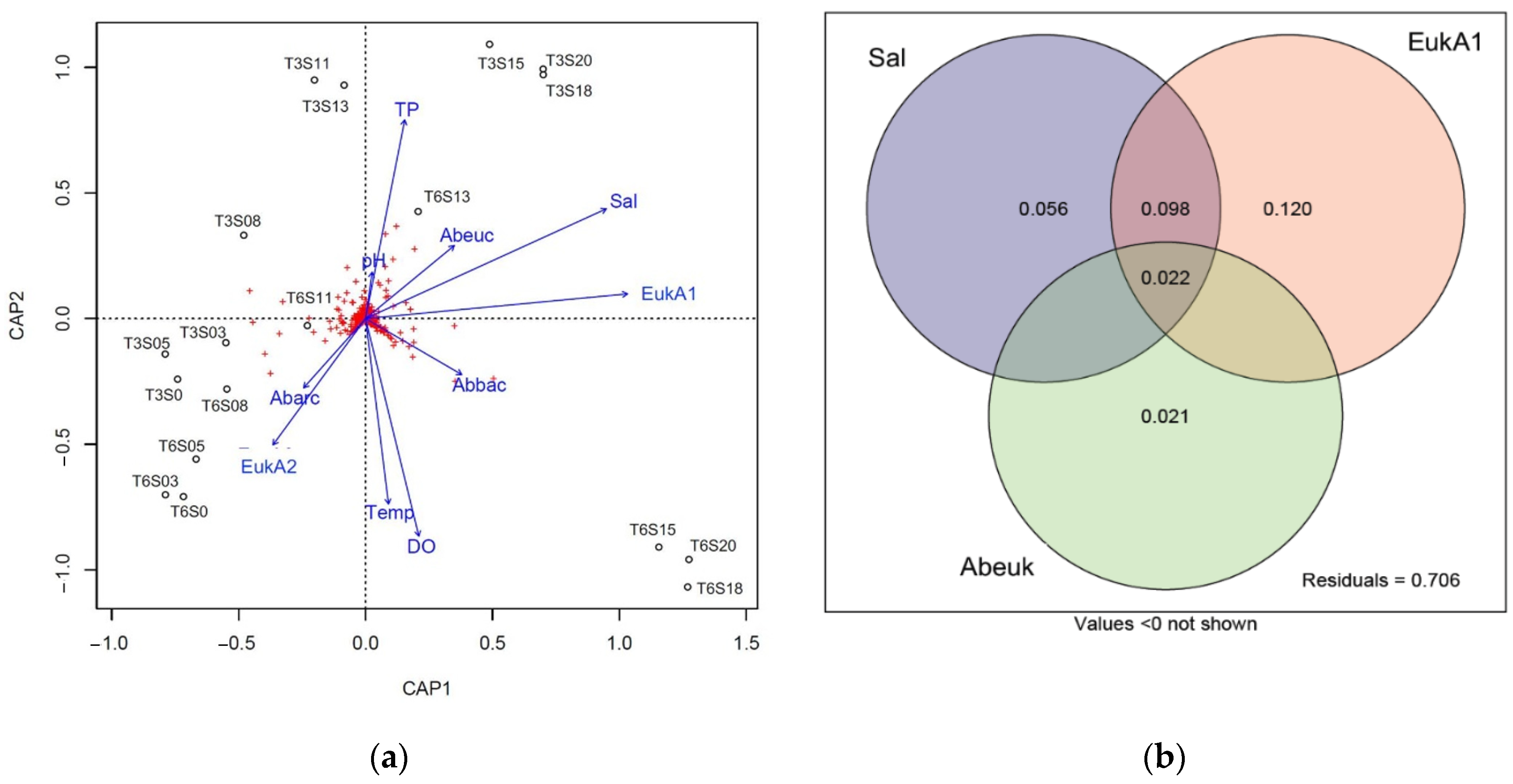
The db-RDA (Figure 2a) indicated that salinity and eukaryotic community composition were strongly and significantly correlated with the bacterial community composition (p = 0.001, Table S6), and that the TP (p = 0.012), temperature (p = 0.017), and absolute abundance of eukaryotes (p = 0.044) were also significantly correlated with bacterial community composition. We used variance partitioning to evaluate the unique and shared contributions of salinity, eukaryotic community composition, and absolute abundance of eukaryotes to bacterial community composition (Figure 2b). Taken together, these factors explained 29.4% of the overall variation, with eukaryotic community composition describing it the best (12%), while salinity explained 5.6%, and absolute abundance of eukaryotes explained 2.1%. Salinity and eukaryotic community composition had shared components explaining 9.8% of the mesocosm bacterial population variation.

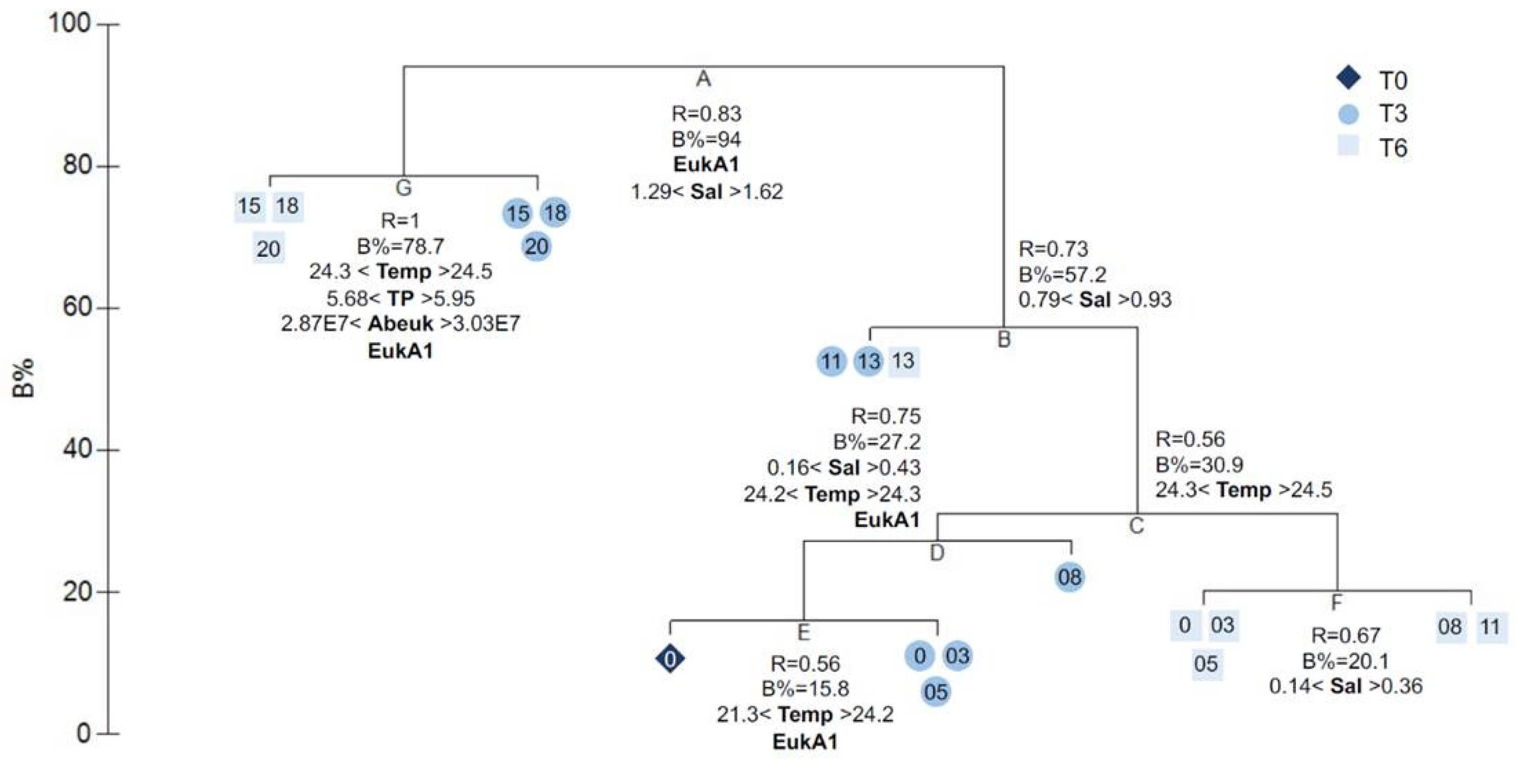
The clustering of samples with the LINKTREE analysis (Figure 3) highlighted a total of seven nodes, which were the regrouped into four clusters (K1, K2, K3, and K4) for further analysis. Node G divided the highest salinity samples at week 3 (T3S15, T3S18, T3S20) and week 6 (T6S15, T6S18, T6S20), which was explained by lower temperatures at week 3 compared to week 6, higher total phosphorus concentrations at week 3, higher eukaryotic absolute abundances at week 3, and differences in eukaryotic community composition. This division was then taken to create cluster K4 and K3. Node A divided the samples between S0–S13 and S15–S20 and was explained by differences in the eukaryotic community composition and higher salinity for samples S15–S20. Node B divided the samples into mid-salinity (T3S11, T3S13, and T6S13) and low salinity (T0, T3S0, T3S05, T3S08, T6S0, T6S03, T6S05, T6S08, and T6S11) and was explained by salinity. Samples T3S11, T3S13, and T6S13 were grouped together to create cluster K2. Nodes C, D, E, and F further divided the samples within the K1 cluster (T0, T3S0, T3S03, T3S05, T3S08, T6S0, T6S03, T6S05, T6S08, and T6S11), which was the group exposed to the lowest salinity. Node C divided the samples from week 3 and week 6 and was explained by lower temperatures at week 3 as compared to week 6. Node D isolated samples T3S08 from samples T0, T3S0, and T3S05 and was explained by salinity, temperature, and eukaryotic community composition differences. Node E further isolated sample T0 from samples T3S0, T3S03, and T3S05 and was explained by a lower temperature at T0 and eukaryotic community composition differences. Finally, node F divided samples T6S0, T6S03, T6S05, T6S08, and T6S11 and was explained by salinity differences. Nodes D, E, and F showed that bacterial community composition in mesocosms exposed to low salinity were closer to the initial freshwater lake community at week 3 than week 6 and is explained mostly by differences in temperature and eukaryotic community composition. A visualization of the dissimilarity (Bray–Curtis) between the bacterial communities by samples and the clustering realized following the Linktree analysis is provided within the framework of a PCoA (Figure S8), with the first axis explaining 33.18% of the variation, while the second axis accounted for 15.36% of the variation.

Salinity groups (based on the four groups defined in the LINKTREE analysis) explained half of the variation in the bacterial mesocosms (PERMANOVA; R² = 0.49, p = 0.001), whereas exposure time explained an additional 11% of the variation (R² = 0.11, p = 0.002) (Table S7), indicating that most of the variation occurring in the mesocosms was due to the addition of salt, and that bacterial populations in each salinity group had distinct community structures.

3.5. Microbial Source Tracking

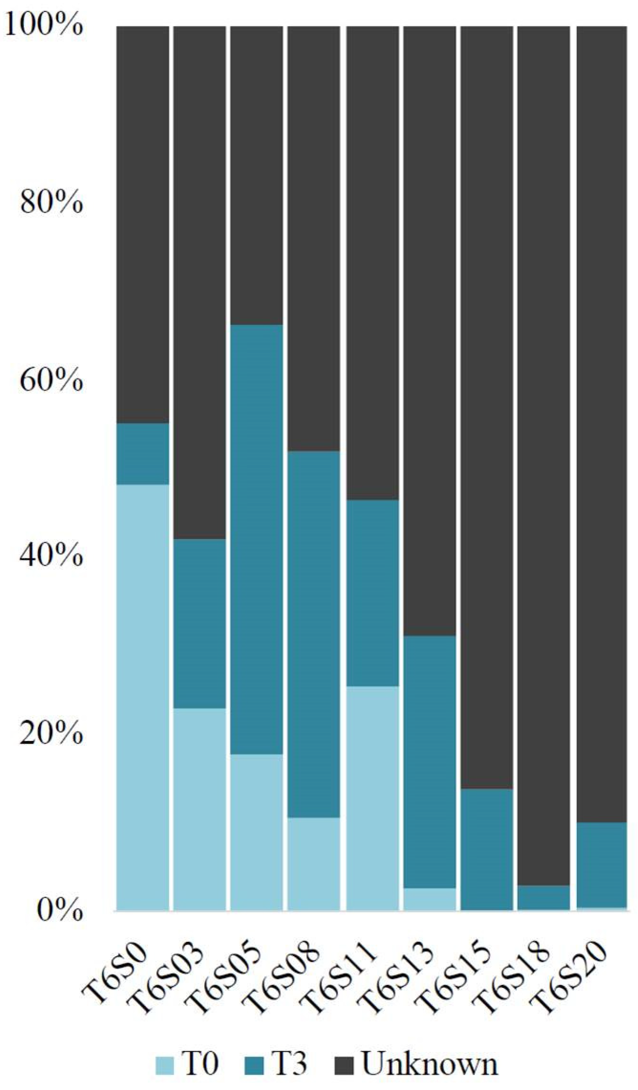
In order to establish the contribution made by the bacterial communities present in the initial water sample (T0) and after three weeks (T3) to those present after six weeks (T6), a fast expectation–maximization microbial source tracking analysis (FEAST) was performed (Figure 4). In mesocosms S0–S13 of T6, a contribution varying between 2.63% and 48.13% was made by the bacterial communities coming from T0, and between 6.98% and 48.55% coming from the communities after three weeks, thus leaving between 33.72% and 68.74% of community contribution associated with an unknown source. For samples S15–S20, little or no (<1%) contribution from T0 communities was observed, and only 2.78–13.88% could be related to the T3 communities, thus leaving between 86.12% and 97.06% having come from an unknown source.

3.6. Significantly Different OTUs between Bacterial Sample Groups

The results of the SIMPER and Kruskal–Wallis analyses carried out on the clusters were identified in the LINKTREE analysis (Table S8). These cluster are K1(T0, T3S0, T3S03, T3S05, T3S08, T6S0, T6S03, T6S05, T6S08, T6S11), K2 (T3S11, T3S13, T6S13), K3 (3S15, T3S18, T3S20), and K4 (T6S15, T6S18, T6S20). The difference in transitional contributors between the four clusters constitutes an indicator of the difference in the mesocosmal community composition as well as their relative abundance. Between cluster K1 and K2, three OTUs associated with Actinobacteria (Frankiales, Micrococcales, Corynebacteriales) were shown to differ significantly, but only two of them remained (Frankiales, Micrococcales) after correction for false discovery rate (fdr). Between clusters K1 and K3, five OTUs associated with Actinobacteria were identified (two Frankiales, two Micrococcales). Two others belonged to the Burkholderiales, and one to Bacteroidia (Flavobacteriales), and two belonged to Alphaproteobacteria (Azospirillales, Ferrovibrionales). Another OTU associated with Gammaproteobacteria (Pseudomonadales) showed a significant differentiation that did not stand after fdr correction. Finally, between K1 and K4, five OTUs associated with Actinobacteria (Micrococcales, Corynebacteriales, three Frankiales), two with Alphaproteobacteria (Rhizobiales, Ferrovibrionales), one with Burkholderiales, and one with Bacteroidia (Cytophagales) were identified as significantly differing between the clusters.

4. Discussion

Our study sought to determine the effect of sodium chloride introduction on freshwater prokaryotic communities. Although microbial community transitions in estuaries are well studied, few of them focus on pristine freshwater environments affected by salinization, particularly at concentrations approaching both Canadian and American chronic and acute chloride exposure regulations. We analyzed the effect generated by the sodium chloride gradient on the absolute abundance, diversity, and structure of archaeal and bacterial communities. To do this, the concentration of Cl⁻ rather than NaCl was considered in order to produce results that are in line with the literature and to better consider the mobility of Cl⁻ [44]. We also chose to include the effect of absolute abundance, the α- and ß-diversities of eukaryotic communities on the prokaryotic communities, as they can be potential predators of prokaryotes and have an impact on their activities [45,46].

4.1. Direct and Indirect Effect of Salinity on Prokaryotic Communities

For the archaea, the values of Cl⁻ explained a very low rate of change in absolute abundance, both after three and six weeks. No significant difference was observed between week 3 and week 6. However, the high absolute abundance observed at the initial time (T0) as compared to the salt-supplemented mesocosms suggests a strong sensitivity to salinization and/or to incubation, as well as the preference of some archaeal taxa for halophily, thermophilia, or a methanogenic lifestyle [47].

Although the absence of archaeal taxa in some samples suggests an overestimation of diversity values, thus making it impossible to rule on the effect of Cl⁻ on archaeal diversity, the analysis of relative abundance nevertheless makes it possible to observe overall trends across the gradient. Among these, it is possible to see the persistence of Nanoarchaeota, present both at T0 and in multiple samples having undergone salt supplementation, even in samples with higher salinity. These organisms—known for their small size and their favoritism for interspecies association [48], or even for their parasitic/ectoparasitic way of life [49]—have been found in several places in the world, and a study by Leoni et al. [50] demonstrated their presence at salinities of up to 145 ppt. It is therefore not surprising to find these organisms at various salinities, even higher ones. Another group present across the gradient, that of the Woesearchaeota, was dominant at very low salinity but also seemed to become more important at higher salinity, while the Bathyarchaeota group was found almost exclusively at the highest salinity samples. Therefore, the Bathyarchaeota has once again contributed to “maintaining the stability and adaptability of the archaeal community” [47], but their global distribution has been linked to total organic carbon (TOC) rather than salinity, according to a study by Yu et al. [51]. On the other hand, the Crenarchaeota, represented by the Nitrosotalea, particularly stood out at lower salinity in T6, where their relative abundance revealed them to be a major taxon. Nevertheless, the presence of these autotrophic ammonia oxidizers is surprising since they would not normally be able to grow in a neutral pH environment [52], whereas the samples taking their presence into account presented a varying pH of between 6.82 and 7.75.

Despite the significative relationship between salinity and bacterial diversity after three and six weeks, very little variability in the diversity indices was observed after both exposure times, with Cl⁻ concentrations explaining 16.6% of the variance of the diversity. Such an effect could be mediated by a variety of factors, including the transition of communities to adapted/acclimatized species. However, as values are proximal and no significant differentiation is present between the sampling times, it could be hypothesized that major succession could have taken place soon after the introduction of NaCl in freshwater (weeks 0–3). Other variables, such as fluctuation in predation pressure and association with eukaryotic species, could have an influence.

An indication of such an effect is shown by the moderate but significant relation of eukaryotic diversity with bacterial diversity after six weeks. However, other factors can induce variations, including viruses, which are known to be a main driver of variation in prokaryotic diversity [45,53].

As for bacterial abundance, our results established that the Cl⁻ levels significantly explained 63% of the variation in bacterial abundance after three weeks. After six weeks, this relationship was significant as well, but it only explained 10% of the variation. Despite there being no significant difference in bacterial abundance between T3 and T6, the observable growth seen through the salinity gradient at both sampling times was indicative of an effect produced by the introduction of NaCl on bacteria into fresh water. Other dynamics can be hypothesized, including the development of taxa adapted to individual mesocosmal conditions over a longer period of time or the development of a top-down system, both of which would promote the general bacterial abundance growth observed throughout the salinity gradient after a 6-week period.

Increased chloride levels could promote the development of bacterial species that benefit from higher salinity and conductivity. The Alphaproteobacteria were significantly positively correlated with the values of Cl⁻, and the observed relative abundance increase of this class across the salinity gradient clearly demonstrates that it benefits from these fluctuations. This effect could, however, be indirect. Bacterial communities may have benefited from the decrease in eukaryotic diversity, which is closely related to the increase in Cl⁻ [54,55,56,57]. This element would prove to be key in Alphaproteobacteria, represented mainly by Rhizobiales and Ferrovibrionales, because these can be heavily consumed by flagellates [58] and can compensate for this phagotrophy by a high cell division. Moreover, these Gram-negative bacteria could particularly benefit from a loss of eukaryotic diversity because some grazing organisms can favor the predation of certain species in particular, according to their size [59], their morphotype [45], but also their composition, by actively avoiding the consumption of Gram-positive species to the detriment of the Gram-negative ones. If the observable loss of diversity suggests predation decline, the joint research carried out by Astorg et al. [6] on the effect generated on eukaryotes showed the clear disappearance of any potential predators across the salinity gradient, in favor of algae belonging to the Ochrophyta group. Most rotifers and other zooplankton taxa were absent from mesocosms at chloride levels higher than 40 mg/L, showing that the benefits brought about by the absence of predators are, however, only one element of a multifactorial environment favoring microbial development, of which the presence of salt is certainly a part when the relative abundances of dominant bacterial taxa are considered.

Conversely, in Actinobacteria, variations were shown to be negatively and significantly correlated with Cl⁻ values. Lower predation pressure (Gram-positive), amplified by their small size [60], would therefore imply that this class was mainly affected by the increasing concentrations of salt rather than predation pressure. A final major group strongly and negatively correlated with Cl⁻ values, and whose relative abundance reflects their importance, is that of Gammaproteobacteria, mainly represented by the Burkholderiales (Betaproteobacteria). Under normal circumstances, the predation of Betaproteobacteria can be thwarted by the production of inedible filaments [58], a strategy necessary to counteract their low rate of division. By combining the existence of a predation escape method and their low division rate with the increase in Cl⁻ levels and the decrease in predation, it seems to be clear that the observable variation of Betaproteobacteria is, at least in part, generated by NaCl addition and not by predation.

Furthermore, as eukaryotic species are affected by the salinity and begin to perish, their decay is mediated by multiple processes, including microbial activity [61]. The involvement of bacterial groups in decomposition processes can contribute to their development, growth, and community transition as well as their overall absolute abundance [62,63]. Indicators of such processes are firstly put forward within the framework of the db-RDA, where it is possible to see the involvement of variables such as TP, eukaryotic abundance, salinity, and eukaryotic beta diversity in the variation of bacterial communities, especially at higher salinities (708.09–1353.73 mg/L Cl⁻). Taken together, the salinity, eukaryotic beta diversity, and eukaryotic absolute abundance explain nearly 30% of the bacterial variance encountered in the mesocosms, and the eukaryotic beta diversity proved to explain the highest proportion of variation (12%) on its own.

These same variables are shown to be, in the context of the LINKTREE analysis, strongly involved in the variations encountered across the gradient, but also between sampling times. Some factors, such as temperature, are involved in the variations encountered but do not vary across the salinity gradient and therefore only represent evidence of the existence of a natural transition of microbial communities during seasonal fluctuations [64] and a demonstration of the incubation time. However, the marked effect of eukaryotic beta diversity on the subdivisions observed across the samples making up the representation of the salinity gradient and time shows that this variable constitutes a key element in the bacterial variation encountered. Although the effect of eukaryotic beta diversity was also present at low salinity, the inclusion of absolute eukaryotic abundance as an explanatory variable for differentiation at higher salinity (≥708.09 mg/L Cl⁻) between T3 and T6 could be an indicator of the dynamics at play. Many bacterial species develop in association with phytoplankton, and some can contribute to the degradation of algal polysaccharides [65]. With a eukaryotic abundance loss of up to 90% at higher salinity between the two sampling times, and with the increased presence of Ochrophyta [6] occupying the higher salinity mesocosms, it can be hypothesized that active and decaying eukaryotic organisms, together with salinity, are among the main influencing factors in the establishment of salt-tolerant bacterial communities.

4.2. Influence of Salinity on Bacterial Community Transition

We sought to determine a threshold salinity concentration from which a significant transition of communities is generated. We observed a differentiation generating four clusters in the LINKTREE analysis, which were also identified within the PCoA of bacterial communities. The first cluster (K1, T0, T3S0, T3S03, T3S05, T3S08, T6S0, T6S03, T6S05, T6S08, and T6S11) consists of mesocosms with bacterial communities proximal to T0 (B% ≤ 30.9), and whose Cl⁻ concentrations reach 354.84 mg/L after having been incubated up to six weeks—concentrations that are greater than the Canadian (120 mg/L Cl⁻) and American (230 mg/L Cl⁻) chronic exposure standards. The proximity of samples up to 354.84 mg/L as compared to the control sample shows that compliance with this standard would ensure the absence of a significant transition of bacterial communities. The communities exposed to Cl⁻ concentrations varying from 420.02 to 572.71 mg/L, mainly for a three-week incubation period, composed a second cluster (K2, T3S11, T3S13, and T6S13) that showed a very highly significant differentiation from the first, low-salinity one. Exposure to Cl⁻ concentrations ranging from 708.09 to 1353.73 mg/L led to the formation of two clusters, one being composed of samples T3S15, T3S18, and T3S20 (K3; 825.45–1353.73 mg/L Cl⁻), while the second was composed of samples T6S15, T6S18, and T6S20 (K4; 708.09–1165.94 mg/L Cl⁻), differing from each other by the duration of exposure to salinity. Although these two higher salinity clusters do not differ significantly from each other, it could be hypothesized that a longer residence time of the ions in the medium would be able to bring such significance. Together, these clusters demonstrate the influence of salinity, with salinity groups explaining as much as 49% of the variation encountered, while exposure time explained 11%.

4.3. Microbial Source Tracking and Overall Procaryotic Transitional Community Trends

As environmental variations are inherent to aquatic habitats, those disturbances can influence the transition of microbial communities [66,67]; a microbial source tracking analysis showed that salinity would greatly influence the resulting composition of such transitions. At lower salinity (0.265–455.585 mg/L Cl⁻), a reasonable contribution (>30%) is made by native communities (T0) and three-week salt-exposed communities (T3) in the community’s composition after a six-week incubation. However, the communities exposed to 511.2 mg/L Cl⁻ or more (T6S15, T6S18, T6S20) are devoid of native communities in their composition (>85% unknown source). Thus, past this threshold, salinized freshwater environments would be highly dependent on the presence of “seed banks” [68,69] in maintaining bacterial diversity and in the transition to halotolerant homologs that may play a role in potential eukaryotic association and decay, as previously mentioned.

An element that should be noted in our overall results is the inclusion of the S11 sample after six weeks of incubation in the first cluster (K1), but also its placement within the LINKTREE and the important contribution made by native communities in its composition (FEAST), suggesting altogether that a partial recovery to “pre-disturbance” communities is not impossible at such salinities, an effect encountered as well by Hu et al. [70] in an extreme salinization–desalinization experiment.

Studies carried out on estuaries [15,16,17] highlight the transition within these systems. Among these, the gradual transition of dominance of Alphaproteobacteria and Gammaproteobacteria at the expense of Actinobacteria and Betaproteobacteria was seen. Unexpectedly, a similar transition of these major groups could be observed in our lake samples and constitute the drivers for significant differentiation between the low and high salinity clusters, as demonstrated by the SIMPER/Kruskal–Wallis analysis. In the differentiation that occurs along the salinity gradient and between clusters, the relative abundance of Actinobacteria has proven to be a key player. As stated above, they were negatively correlated with Cl⁻ values and were noticeably present within the framework of the aforementioned Simper/Kruskal–Wallis analysis. As samples collected are but a part of the total community within the mesocosm, there is no doubt that more species can be affected by NaCl introduction, in our study and in the natural habitat, and that the observed effect throughout the salinity gradient could potentially increase with time and with increasing salinity. While the bacterial transition in estuaries is majorly driven by hydrologic conditions [16] and the spring–neap tidal cycle [71], the implication of nutrient supply variations is nonetheless intrinsic to those notions. As freshwater lakes tend to have a longer residence time, and that a link between microbial development, salinity, time, and potentially eukaryotic decay was present in our study, the implication of nutrient fluctuations in community changes could represent a good research path to really understand the effect of the freshwater salinization syndrome on microbial communities. Considering the increase in Alphaproteobacteria at higher salinity, with Rhizobiales as the main members, and that the latter may be associated with an increase in nutrients with the potential to induce acidification and hypoxia in oceanic environments [72], carrying out a longer-term study could also be appropriate to better consider the issues encountered in understanding the effect of salinity on microbial communities in lake environments.

5. Conclusions

Overall, no clear linearity between the introduction of NaCl and prokaryotic diversity was present in our study after three and six weeks. However, a positive relationship appears to be present between NaCl and absolute bacterial abundance after three weeks. An increase in abundance was seen and amplified over time. Salinity clearly plays an important role in the observed bacterial abundance increase, and so do other potential factors such as loss of eukaryotic diversity and the potentially associated decomposition. While our results show the effect of salinity on prokaryotic organisms, they also raise the existence of multifactorial dynamics. Some taxa may potentially be directly affected by salinity levels (i.e., Actinobacteria, Burkholderiales), while others (i.e., Alphaproteobacteria, Rhizobiales, Ferrovibrionales) could benefit from the loss of predation brought about by the loss of eukaryotic diversity. However, the increase in Ochrophyta, as demonstrated by the joint study by Astorg et al. [6], also leaves room for potential associations between prokaryotes and phytoplanktons, active or decaying; the variance explained by eukaryotic beta diversity on bacterial community variations suggests the same.

Furthermore, we were also able to observe that a significant transition in bacterial communities was present from a threshold of 420.02 mg/L Cl⁻, a level higher than the Canadian (120 mg/L Cl⁻) and American (230 mg/L Cl⁻) recommendations in terms of chronic exposure, and also higher than the sensitivity threshold of other organisms (i.e., zooplankton). Thus, compliance with the standards in place would be able to ensure the sustainability of freshwater prokaryotic communities. While other transition thresholds were present, those operated at higher salinity suggest that they would not be possible without the presence of seed banks. Conversely, we did observe a partial recovery of “pre-disturbance” freshwater bacterial communities during a drop in salinity, which could only have been possible through “native” communities capable of resilience. Finally, a transition of dominance by Actinobacteria and Betaproteobacteria towards Alphaproteobacteria and Gammaproteobacteria could be observed during our study, which is in part similar to the results obtained in the context of studies carried out in estuaries. Although these results hint at a possible long-term effect, consideration of nutrient variations in further studies may be essential to better understand the effect of freshwater salinization on microbial communities. Overall, our results, combined with those of Astorg et al. [6] and derived from the same mesocosm experiment, suggest that eukaryotic communities would therefore be more sensitive to salt intrusion in freshwater environments. As a result, these would be better indicators of the salinization of fresh waters, particularly in view of the multiplicity of taxa substituting native prokaryote communities and the transitional tolerance threshold associated with theprocaryotes as compared to eukaryotes. Understanding all the effects caused by the intrusion of NaCl on trophic webs could, in the long term, make it possible to recognize the warning signs of larger-scale freshwater salinization and its drastic effects, both ecologic and economic.

References

- Gouvernement of Canada. Code de Pratique de la Gestion Environnementale des sels de Voirie. 2018. Available online: https://www.canada.ca/fr/environnement-changement-climatique/services/polluants/sels-voirie/code-pratique-gestion-environnementale.html (accessed on 18 September 2020).
- Schuler, M.S.; Cañedo-Argüelles, M.; Hintz, W.D.; Dyack, B.; Birk, S.; Relyea, R.A. Regulations are needed to protect freshwater ecosystems from salinization. Philos. Trans. R. Soc. B Biol. Sci. 2018, 374, 20180019. [Google Scholar] [CrossRef] [PubMed] [Green Version]
- CCME-Canadian Council of Ministers of the Environment. Scientific Criteria Document for the Development of the Canadian Water Quality Guidelines for the Protection of Aquatic Life: Chloride Ion; Canadian Council of Ministers of the Environment: Winnipeg, BC, Canada, 2011; ISBN 9781-896997-77-3. PN 1460. [Google Scholar]
- Galella, J.G.; Kaushal, S.; Wood, K.L.; Reed, L. Freshwater Salinization Syndrome: Anthropogenic effects of road salting over land use and time. In AGU Fall Meeting Abstracts; American, Geophysical Union: Washington, DC, USA, 2019; p. H43Q-2319. [Google Scholar]
- Kelly, V.R.; Findlay, S.E.G.; Weathers, K.C. Road Salt: The Problem, the Solution, and How to Get There; Cary Institute of Ecosystem Studies: Millbrook, NY, USA, 2019. [Google Scholar]
- Astorg, L.; Gagnon, J.; Lazar, C.S.; Derry, A.M. Effects of freshwater salinization on a salt-naïve planktonic eukaryote community. Limnol. Oceanogr. Lett. 2022. [Google Scholar] [CrossRef]
- Lionard, M.; Muylaert, K.; Gansbeke, D.V.; Vyverman, W. Influence of changes in salinity and light intensity on growth of phytoplankton communities from the Schelde river and estuary (Belgium/The Netherlands). Hydrobiologia 2005, 540, 105–115. [Google Scholar] [CrossRef]
- Tavsanoglu, U.N.; Maleki, R.; Akbulut, N. Effects of Salinity on the Zooplankton Community Structure in Two Maar Lakes and One Freshwater Lake in the Konya Closed Basin, Turkey. Ekoloji Derg. 2015, 24, 25–32. [Google Scholar] [CrossRef]
- Franceschini, J. Exploring the Impacts of Increased Salinity on Zooplankton Communities in Sturgeon Lake. Bachelor’s Thesis, Wilfrid Laurier University, Waterloo, ON, Canada, 2019. [Google Scholar]
- Moffett, E.R.; Baker, H.K.; Bonadonna, C.C.; Shurin, J.B.; Symons, C.C. Cascading effects of freshwater salinization on plankton communities in the Sierra Nevada. Limnol. Oceanogr. Lett. 2020, 2. [Google Scholar] [CrossRef]
- Nielsen, D.L.; Brock, M.A.; Vogel, M.; Petrie, R. From fresh to saline: A comparison of zooplankton and plant communities developing under a gradient of salinity with communities developing under constant salinity levels. Mar. Freshw. Res. 2008, 59, 549–559. [Google Scholar] [CrossRef]
- Hintz, W.D.; Jones, D.K.; Relyea, R.A. Evolved tolerance to freshwater salinization in zooplankton: Life-history trade-offs, cross-tolerance and reducing cascading effects. Philos. Trans. R. Soc. B Biol. Sci. 2018, 374, 20180012. [Google Scholar] [CrossRef] [Green Version]
- Coldsnow, K.D.; Mattes, B.M.; Hintz, W.D.; Relyea, R.A. Rapid evolution of tolerance to road salt in zooplankton. Environ. Pollut. 2017, 222, 367–373. [Google Scholar] [CrossRef]
- Ishika, T.; Bahri, P.A.; Laird, D.W.; Moheimani, N.R. The effect of gradual increase in salinity on the biomass productivity and biochemical composition of several marine, halotolerant, and halophilic microalgae. J. Appl. Phycol. 2018, 30, 1453–1464. [Google Scholar] [CrossRef]
- Cottrell, M.; Kirchman, D. Single-cell analysis of bacterial growth, cell size, and community structure in the Delaware estuary. Aquat. Microb. Ecol. 2004, 34, 139–149. [Google Scholar] [CrossRef] [Green Version]
- Bouvier, T.C.; del Giorgio, P. Compositional changes in free-living bacterial communities along a salinity gradient in two temperate estuaries. Limnol. Oceanogr. 2002, 47, 453–470. [Google Scholar] [CrossRef]
- Herlemann, D.P.R.; Labrenz, M.; Jürgens, K.; Bertilsson, S.; Waniek, J.J.; Andersson, A.F. Transitions in bacterial communities along the 2000 km salinity gradient of the Baltic Sea. ISME J. 2011, 5, 1571–1579. [Google Scholar] [CrossRef] [Green Version]
- Henriques, I.S.; Alves, A.; Tacão, M.; Almeida, A.; Cunha, A.; Correia, A. Seasonal and spatial variability of free-living bacterial community composition along an estuarine gradient (Ria de Aveiro, Portugal). Estuar. Coast. Shelf Sci. 2006, 68, 139–148. [Google Scholar] [CrossRef]
- Bartolomé, M.C.; D’ors, A.; Sánchez-Fortún, S. Toxic effects induced by salt stress on selected freshwater prokaryotic and eukaryotic microalgal species. Ecotoxicology 2009, 18, 174–179. [Google Scholar] [CrossRef] [PubMed]
- Kartal, B.; Koleva, M.; Arsov, R.; van der Star, W.; Jetten, M.S.; Strous, M. Adaptation of a freshwater anammox population to high salinity wastewater. J. Biotechnol. 2006, 126, 546–553. [Google Scholar] [CrossRef] [PubMed]
- Kaushal, S.S.; Likens, G.E.; Pace, M.L.; Reimer, J.E.; Maas, C.M.; Galella, J.G.; Utz, R.M.; Duan, S.; Kryger, J.R.; Yaculak, A.M.; et al. Freshwater salinization syndrome: From emerging global problem to managing risks. Biodegradation 2021, 154, 255–292. [Google Scholar] [CrossRef]
- Kaushal, S.S.; Groffman, P.M.; Likens, G.E.; Belt, K.T.; Stack, W.P.; Kelly, V.R.; Band, L.E.; Fisher, G.T. Increased salinization of fresh water in the northeastern United States. Proc. Natl. Acad. Sci. USA 2005, 102, 13517–13520. [Google Scholar] [CrossRef] [Green Version]
- Dugan, H.A.; Bartlett, S.L.; Burke, S.M.; Doubek, J.P.; Krivak-Tetley, F.E.; Skaff, N.K.; Summers, J.C.; Farrell, K.J.; McCullough, I.M.; Morales-Williams, A.M.; et al. Salting our freshwater lakes. Proc. Natl. Acad. Sci. USA 2017, 114, 4453–4458. [Google Scholar] [CrossRef] [Green Version]
- Statistics Canada. Canada’s Core Public Infrastructure Survey: Interactive Dashboard. Gouvernement du Canada, 2018. Available online: https://www150.statcan.gc.ca/n1/pub/71-607-x/71-607-x2021002-eng.htm (accessed on 26 October 2020).
- Wetzel, R.G.; Likens, G.E. Limnological Analyses, 3rd ed.; Springer Press: New York, NY, USA, 2000; pp. 97–98. ISBN 978-1-4757-3250-4. [Google Scholar] [CrossRef]
- Pfaff, J.D. Method 300.0 Determination of Inorganic Anions by Ion Chromatography; US Environmental Protection Agency, Office of Research and Development, Environmental Monitoring Systems Laboratory: Cincinnati, OH, USA, 1993. [Google Scholar]
- Qiagen. DNeasy® PowerWater® Kit Handbook; HB-2267-001 © 2017; QIAGEN: Hilden, Germany, 2017; all rights reserved. [Google Scholar]
- ThermoFisher Scientific. N.D. QuantStudio™ 3D Digital PCR System User Manual; Applied Biosystems: Waltham, MA, USA, 2021; PN MAN0007720; Available online: https://assets.thermofisher.com/TFS-Assets/LSG/manuals/MAN0007720.pdf (accessed on 20 January 2019).
- ThermoFisher Scientific. Target Quantification Using SYBR® Green I Dye on the QuantStudio™ 3D Digital PCR System; Demonstrated Protocol; Applied Biosystems: Waltham, MA, USA, 2014; CO35063 0414. [Google Scholar]
- Sun, Y.; Zhong, S.; Deng, B.; Jin, Q.; Wu, J.; Huo, J.; Zhu, J.; Zhang, C.; Li, Y. Impact of Phellinus gilvus mycelia on growth, immunity and fecal microbiota in weaned piglets. PeerJ 2020, 8, e9067. [Google Scholar] [CrossRef]
- Lazar, C.; Stoll, W.; Lehmann, R.; Herrmann, M.; Schwab, V.F.; Akob, D.M.; Nawaz, A.; Wubet, T.; Buscot, F.; Totsche, K.-U.; et al. Archaeal Diversity and CO2Fixers in Carbonate-/Siliciclastic-Rock Groundwater Ecosystems. Archaea 2017, 2017, 2136287. [Google Scholar] [CrossRef] [Green Version]
- Schloss, P.D.; Westcott, S.L.; Ryabin, T.; Hall, J.R.; Hartmann, M.; Hollister, E.B.; Lesniewski, R.A.; Oakley, B.B.; Parks, D.H.; Robinson, C.J.; et al. Introducing mothur: Open-Source, Platform-Independent, Community-Supported Software for Describing and Comparing Microbial Communities. Appl. Environ. Microbiol. 2009, 75, 7537–7541. [Google Scholar] [CrossRef] [PubMed] [Green Version]
- Liu, X.; Li, M.; Castelle, C.; Probst, A.; Zhou, Z.; Pan, J.; Liu, Y.; Banfield, J.; Gu, J.-D. Insights into the ecology, evolution, and metabolism of the widespread Woesearchaeotal lineages. Microbiome 2018, 6, 102. [Google Scholar] [CrossRef] [PubMed]
- Zhou, Z.; Pan, J.; Wang, F.; Gu, J.-D.; Li, M. Bathyarchaeota: Globally distributed metabolic generalists in anoxic environments. FEMS Microbiol. Rev. 2018, 42, 639–655. [Google Scholar] [CrossRef]
- Team, R. RStudio: Integrated Development for R. RStudio, Inc. Available online: http://www.rstudio.com (accessed on 20 January 2019).
- McMurdie, P.J.; Holmes, S. phyloseq: An R package for reproducible interactive analysis and graphics of microbiome census data. PLoS ONE 2013, 8, e61217. [Google Scholar] [CrossRef] [PubMed] [Green Version]
- Smith, S. Phylosmith: An R-package for reproducible and efficient microbiome analysis with phyloseq-objects. J. Open Source Softw. 2019, 4, 1442. [Google Scholar] [CrossRef]
- Clarke, K.R.; Gorley, R.N. PRIMER v6. User manual/tutorial. In Plymouth Routine in Mulitvariate Ecological Research; Plymouth Marine Laboratory: Plymouth, UK, 2006. [Google Scholar]
- Clarke, K.; Green, R. Statistical design and analysis for a ’biological effects’ study. Mar. Ecol. Prog. Ser. 1988, 46, 213–226. [Google Scholar] [CrossRef]
- Clarke, K.R.; Somerfield, P.; Gorley, R.N. Testing of null hypotheses in exploratory community analyses: Similarity profiles and biota-environment linkage. J. Exp. Mar. Biol. Ecol. 2008, 366, 56–69. [Google Scholar] [CrossRef]
- Oksanen, J. Multivariate Analysis of Ecological Communities in R: Vegan Tutorial; Univ. of Oulu: Oulu, FI, USA, 2007. [Google Scholar]
- Steinberger, A. Asteinberger9/Seq_Scripts, Version v1.1; Zenodo, 2020. Available online: https://zenodo.org/record/4270481#.YoXBqqBByUk (accessed on 20 January 2019). [CrossRef]
- Shenhav, L.; Thompson, M.; Joseph, T.A.; Briscoe, L.; Furman, O.; Bogumil, D.; Mizrahi, I.; Pe’er, I.; Halperin, E. FEAST: Fast expectation-maximization for microbial source tracking. Nat. Methods 2019, 16, 627–632. [Google Scholar] [CrossRef]
- MTQ. Ministère des transports du Québec Stratégie québécoise pour une gestion environnementale des sels de voirie. In Direction de L’environnement et de la Recherche; Dépôt Légal—Bibliothèque et Archives Nationales du Québec; Publications du Québec: Montréal, QC, Canada, 2019; ISBN 978-2-550-60045. [Google Scholar]
- Pernthaler, J. Predation on prokaryotes in the water column and its ecological implications. Nat. Rev. Microbiol. 2005, 3, 537–546. [Google Scholar] [CrossRef]
- Jousset, A. Ecological and evolutive implications of bacterial defences against predators. Environ. Microbiol. 2011, 14, 1830–1843. [Google Scholar] [CrossRef]
- Zou, D.; Liu, H.; Li, M. Community, Distribution, and Ecological Roles of Estuarine Archaea. Front. Microbiol. 2020, 11, 2060, PMCID: PMC7484942. [Google Scholar] [CrossRef] [PubMed]
- John, E.S.; Reysenbach, A.L. Nanoarchaeota. In Encyclopedia of Microbiology, 4th ed.; Academic Press: Cambridge, MA, USA, 2019; pp. 274–279. ISBN 9780128117378. [Google Scholar]
- Jarrell, K.F.; Albers, S.J. Archaellum. In Encyclopedia of Microbiology, 4th ed.; Academic Press: Cambridge, MA, USA, 2019; pp. 253–261. ISBN 9780128117378. [Google Scholar]
- Leoni, C.; Volpicella, M.; Fosso, B.; Manzari, C.; Piancone, E.; Dileo, M.C.G.; Arcadi, E.; Yakimov, M.; Pesole, G.; Ceci, L.R. A Differential Metabarcoding Approach to Describe Taxonomy Profiles of Bacteria and Archaea in the Saltern of Margherita di Savoia (Italy). Microorganisms 2020, 8, 936. [Google Scholar] [CrossRef] [PubMed]
- Yu, T.; Liang, Q.; Niu, M.; Wang, F. High occurrence of Bathyarchaeota (MCG) in the deep-sea sediments of South China Sea quantified using newly designed PCR primers. Environ. Microbiol. Rep. 2017, 9, 374–382. [Google Scholar] [CrossRef] [PubMed]
- Prosser, J.I.; Nicol, G.W. Candidatus nitrosotalea. In Bergey’s Man. Syst. Archaea Bact. April; 2015; pp. 1–7. ISBN 9781118960608. [Google Scholar] [CrossRef]
- Tang, B.-L.; Yang, J.; Chen, X.-L.; Wang, P.; Zhao, H.-L.; Su, H.-N.; Li, C.-Y.; Yu, Y.; Zhong, S.; Wang, L.; et al. A predator-prey interaction between a marine Pseudoalteromonas sp. and Gram-positive bacteria. Nat. Commun. 2020, 11, 285. [Google Scholar] [CrossRef] [PubMed]
- Dickman, M.; Gochnauer, M. Impact of sodium chloride on the microbiota of a small stream. Environ. Pollut. (1970) 1978, 17, 109–126. [Google Scholar] [CrossRef]
- Cañedo-Argüelles, M.; Kefford, B.; Piscart, C.; Prat, N.; Schäfer, R.; Schulz, C.-J. Salinisation of rivers: An urgent ecological issue. Environ. Pollut. 2013, 173, 157–167. [Google Scholar] [CrossRef]
- Cañedo-Argüelles, M.; Hawkins, C.P.; Kefford, B.J.; Schäfer, R.B.; Dyack, B.J.; Brucet, S.; Buchwalter, D.; Dunlop, J.; Frör, O.; Lazorchak, J.; et al. Saving freshwater from salts. Science 2016, 351, 914–916. [Google Scholar] [CrossRef]
- Environment Canada. Priority Substances List Assessment Report: Road Salts. In Canadian Environmental Protection Act 1999; Environment Canada: Ottawa, ON, Canada, 2001; ISBN 0-662-31018-7. [Google Scholar]
- Pernthaler, J.; Posch, T.; Simek, K.; Vrba, J.; Amann, R.; Psenner, R. Contrasting bacterial strategies to coexist with a flagellate predator in an experimental microbial assemblage. Appl. Environ. Microbiol. 1997, 63, 596–601. [Google Scholar] [CrossRef] [Green Version]
- Gonzalez, J.M.; Sherr, E.B.; Sherr, B.F. Size-selective grazing on bacteria by natural assemblages of estuarine flagellates and ciliates. Appl. Environ. Microbiol. 1990, 56, 583–589. [Google Scholar] [CrossRef] [Green Version]
- Jezbera, J.; Horňák, K.; Imek, K. Food selection by bacterivorous protists: Insight from the analysis of the food vacuole content by means of fluorescence in situ hybridization. FEMS Microbiol. Ecol. 2005, 52, 351–363. [Google Scholar] [CrossRef] [Green Version]
- Jackrel, S.; Gilbert, J.A.; Wootton, J.T. The Origin, Succession, and Predicted Metabolism of Bacterial Communities Associated with Leaf Decomposition. mBio 2019, 10, e01703-19. [Google Scholar] [CrossRef] [PubMed] [Green Version]
- Alonso, C.; Warnecke, F.; Amann, R.; Pernthaler, J. High local and global diversity of Flavobacteria in marine plankton. Environ. Microbiol. 2007, 9, 1253–1266. [Google Scholar] [CrossRef] [PubMed]
- Kirchman, D.L. The ecology of Cytophaga-Flavobacteria in aquatic environments. FEMS Microbiol. Ecol. 2002, 39, 91–100. [Google Scholar] [CrossRef]
- Zhu, C.; Zhang, J.; Nawaz, M.Z.; Mahboob, S.; Al-Ghanim, K.A.; Khan, I.A.; Lu, Z.; Chen, T. Seasonal succession and spatial distribution of bacterial community structure in a eutrophic freshwater Lake, Lake Taihu. Sci. Total Environ. 2019, 669, 29–40. [Google Scholar] [CrossRef]
- Goecke, F.R.; Thiel, V.; Wiese, J.; Labes, A.; Imhoff, J.F. Algae as an important environment for bacteria–phylogenetic relationships among new bacterial species isolated from algae. Phycologia 2013, 52, 14–24. [Google Scholar] [CrossRef]
- Shabarova, T.; Salcher, M.M.; Porcal, P.; Znachor, P.; Nedoma, J.; Grossart, H.-P.; Seďa, J.; Hejzlar, J.; Šimek, K. Recovery of freshwater microbial communities after extreme rain events is mediated by cyclic succession. Nat. Microbiol. 2021, 6, 479–488. [Google Scholar] [CrossRef]
- Li, H.; Barber, M.; Lu, J.; Goel, R. Microbial community successions and their dynamic functions during harmful cyanobacterial blooms in a freshwater lake. Water Res. 2020, 185, 116292. [Google Scholar] [CrossRef]
- Lennon, J.T.; Jones, S.E. Microbial seed banks: The ecological and evolutionary implications of dormancy. Nat. Rev. Genet. 2011, 9, 119–130. [Google Scholar] [CrossRef]
- Wisnoski, N.I.; Lennon, J.T. Stabilising role of seed banks and the maintenance of bacterial diversity. Ecol. Lett. 2021, 24, 2328–2338. [Google Scholar] [CrossRef]
- Hu, Y.; Bai, C.; Cai, J.; Shao, K.; Tang, X.; Gao, G. Low recovery of bacterial community after an extreme salinization-desalinization cycle. BMC Microbiol. 2018, 18, 195. [Google Scholar] [CrossRef]
- Khandeparker, L.; Eswaran, R.; Gardade, L.; Kuchi, N.; Mapari, K.; Naik, S.D.; Anil, A.C. Elucidation of the tidal influence on bacterial populations in a monsoon influenced estuary through simultaneous observations. Environ. Monit. Assess. 2016, 189, 41. [Google Scholar] [CrossRef] [PubMed]
- Lemos, L.N.; de Carvalho, F.M.; Gerber, A.; Guimarães, A.P.C.; Jonck, C.R.; Ciapina, L.P.; de Vasconcelos, A.T.R. Genome-centric metagenomics reveals insights into the evolution and metabolism of a new free-living group in Rhizobiales. BMC Microbiol. 2021, 21, 294. [Google Scholar] [CrossRef] [PubMed]
Figure 1.
(a) Regression of bacterial absolute abundance and chloride (Cl−) in mesocosms at T3 and T6. (b) Regression of bacterial diversity (Shannon’s H) and Cl− in mesocosms after three (T3) and six weeks (T6) of exposure.
Figure 2.
(a) Correlation between the bacterial mesocosm community composition and explanatory factors using distance-based redundancy analysis (db-RDA). T3, 3-week exposure to the salinity gradient; T6, 6-week exposure; TP, total phosphorus; Sal, salinity; Temp, temperature; DO, dissolved oxygen; Abarc, absolute abundance of archaea; Abbac, absolute abundance of bacteria; Abeuk, absolute abundance of eukaryotes; EukA1, eukaryotic community composition represented by the first axis of a PCoA; EukA2, eukaryotic community composition represented by the second axis of a principal coordinates analysis (PCoA). (b) Variance partitioning analysis separating variation in the bacterial mesocosm community composition between 3 explanatory variables: salinity (Sal), eukaryotic community composition represented by the first axis of a PCoA (EukA1), and absolute abundance of eukaryotes (Abeuk). Values represent the portion of variation explained by the explanatory variables.
Figure 3.
Linkage tree analysis showing the clustering of bacterial mesocosm samples constrained by significant explanatory variables: TP, total phosphorus; Sal, salinity; Temp, temperature; Abeuk, absolute abundance of eukaryotes; EukA1, eukaryotic community composition represented by the first axis of a PCoA. For each cluster, R is the optimal analysis of similarities (ANOSIM) R value (relative subgroup separation). The B% axis shows the absolute group separation, which is scaled to maximum for the first division.
Figure 4.
Bacterial source tracking of bacterial samples from week 6, carried out using fast expectation–maximization microbial source tracking analysis (FEAST). The source samples are the initial freshwater lake sample used to set up the mesocosms (T0), and the samples for each bag at week 3 (T3).
Publisher’s Note: MDPI stays neutral with regard to jurisdictional claims in published maps and institutional affiliations. |
© 2022 by the authors. Licensee MDPI, Basel, Switzerland. This article is an open access article distributed under the terms and conditions of the Creative Commons Attribution (CC BY) license (https://creativecommons.org/licenses/by/4.0/).
Share and Cite
MDPI and ACS Style
Gagnon, J.-C.; Astorg, L.; Derry, A.M.; Lazar, C.S. Response of Prokaryotic Communities to Freshwater Salinization. Appl. Microbiol. 2022, 2, 330-346. https://doi.org/10.3390/applmicrobiol2020025
AMA Style
Gagnon J-C, Astorg L, Derry AM, Lazar CS. Response of Prokaryotic Communities to Freshwater Salinization. Applied Microbiology. 2022; 2(2):330-346. https://doi.org/10.3390/applmicrobiol2020025
Chicago/Turabian StyleGagnon, Jean-Christophe, Louis Astorg, Alison M. Derry, and Cassandre Sara Lazar. 2022. "Response of Prokaryotic Communities to Freshwater Salinization" Applied Microbiology 2, no. 2: 330-346. https://doi.org/10.3390/applmicrobiol2020025