Improving Localization of Deep Inclusions in Time-Resolved Diffuse Optical Tomography

Abstract

Time-resolved diffuse optical tomography is a technique used to recover the optical properties of an unknown diffusive medium by solving an ill-posed inverse problem. In time-domain, reconstructions based on datatypes are used for their computational efficiency. In practice, most used datatypes are temporal windows and Fourier transform. Nevertheless, neither theoretical nor numerical studies assessing different datatypes have been clearly expressed. In this paper, we propose an overview and a new process to compute efficiently a long set of temporal windows in order to perform diffuse optical tomography. We did a theoretical comparison of these large set of temporal windows. We also did simulations in a reflectance geometry with a spherical inclusion at different depths. The results are presented in terms of inclusion localization and its absorption coefficient recovery. We show that (1) the new windows computed with the developed method improve inclusion localization for inclusions at deep layers, (2) inclusion absorption quantification is improved at all depths and, (3) in some cases these windows can be equivalent to frequency based reconstruction at GHz order.

1. Introduction

Time-resolved diffuse optical technology is an emerging photonic technique to continuously quantify the concentrations of several physiological chromophores such as hemoglobin, lipid or collagen. Successful measurements have been done at different human body locations such as brain [1,2], breast [3] or thyroid [4]. An interesting extension of this technology is to perform diffuse optical tomography [5,6] by computing three-dimensional maps of oxy- and deoxy-hemoglobin; in this approach, photon propagation is modeled in a computer and results are compared with experimental measurements. Then, optical parameters in the model are updated by solving an ill-posed inverse problem until the difference between the model and the data is negligible.

In order to have accurate results, it is important to have a realistic model for photon propagation in tissues. The most accurate approach is to use the integro-differential Radiative Transfer Equation (RTE) [7]. Although RTE has some analytical solutions [8,9,10] these just hold for simple geometries and cannot be applied to more complex environments, such as an human head or breast models, without making strong assumptions. Apart from classical Monte-Carlo simulations [11,12], new numerical methods have been proposed, some of which are the one-way RTE [13] or hybrid RTE [14]; nevertheless, they are still highly time-consuming for real-time applications.

Due to the previous reasons, usually the first-order time-dependant Diffusion Approximation is used,

$$\frac{1}{c}\frac{\partial \varphi (\mathbf{r},t)}{\partial t}-\nabla ·(D\left(\mathbf{r}\right)\nabla \varphi (\mathbf{r},t))+{\mu }_a\left(\mathbf{r}\right)\varphi (\mathbf{r},t)=S(\mathbf{r},t),$$

(1)

where c is the speed of light in the medium, $\varphi$ is the fluence rate, $D={\left(3{\mu }_s^{\prime }\right)}^{-1}$ [15,16], ${\mu }_a$ and ${\mu }_s^{\prime }$ are the diffusion, absorption and reduced scattering coefficients respectively, and S is the source function. This approximation, based on spherical harmonics [7], is valid assuming that (1) the reduced scattering coefficient is much greater than absorption (${\mu }_s^{\prime }\gg {\mu }_a$) and that (2) detectors are sufficiently far from light sources (>$10/{\mu }_s^{\prime }$). These assumptions hold in most practical cases and although higher order approximations have also been suggested [17,18,19] the extra computational cost usually does not compensate the small gain in accuracy.

The time-dependant Equation (1) can be solved using Finite Element Method [20] but it is still a slow process since time has to be discretized in short steps in order to guarantee stability and convergence. For this reason, several authors have proposed to use temporal windows datatypes since they are faster to compute than the fluence rate itself [21,22]. Nevertheless, as indicated in [23], the temporal windows datatypes are faster to compute than the fluence rate if they have the form $w\left(t\right)=t^n{e}^{-pt}$ where $n\in \mathbb{N}$ is in the set of natural numbers and $p\in \mathbb{C}$ is in the set of complex numbers. This formula incorporates the Fourier transform (when $n=0$ and p is an imaginary number), Laplace transform (when $n=0$ and p is a complex number), standard moments (when n is an integer and $p=0$) and Mellin-Laplace moments (when n is an integer and p is a real number).

Some authors prefer to use Fourier Transform (FT) datatypes. In [2] the magnitude and phase of 100 MHz frequency from a time-resolved signal was used for the reconstruction. A similar approach was published in [24] to retrieve the fluorescence lifetime distribution. A related idea is to directly use frequency-domain technology [25,26,27] to retrieve optical properties or fluorescence lifetime [28,29]. These reconstruction approaches based on solving the inverse problem in frequency domain are a good alternative to temporal windows but are not equivalent since only MHz order frequencies are used.

In this paper, we propose a new technique for computing fluence rate temporal windows datatypes without constraining ourselves to $w\left(t\right)=t^n{e}^{-pt}$ form and preserving low computing times. We analyse different types of windows in terms of temporal selectivity, noise influence and computational efficiency. Described datatypes are compared in simulations with respect to the state-of-the-art reconstruction technique. Finally, we reformulate the new method as a frequency based reconstruction using up to GHz order.

2. Methods

In this section, an introduction to time- and datatypes-based reconstruction will be given and a new method for computing temporal windows will be described. Further on, different temporal windows and their noise influence on reconstruction methods will be studied. After, the setup of the numerical simulations are presented.

2.1. Time- and Datatypes-Based Reconstruction

Time-resolved diffuse optical tomography can be posed in terms of time bins or datatypes; in both cases time-resolved measurements from the detectors are used. Absorption of the medium $\Omega$ can be recovered by using iteratively the linearized Born approximation,

$$\delta {\varphi }_{sd}\left(t\right)={\int }_{\Omega }\left[{\varphi }_s^{\left(k\right)}\ast G_d^{\left(k\right)}\right](\mathbf{r},t)\delta {\mu }_a^{\left(k\right)}\left(\mathbf{r}\right)\mathrm{d}\mathbf{r},$$

(2)

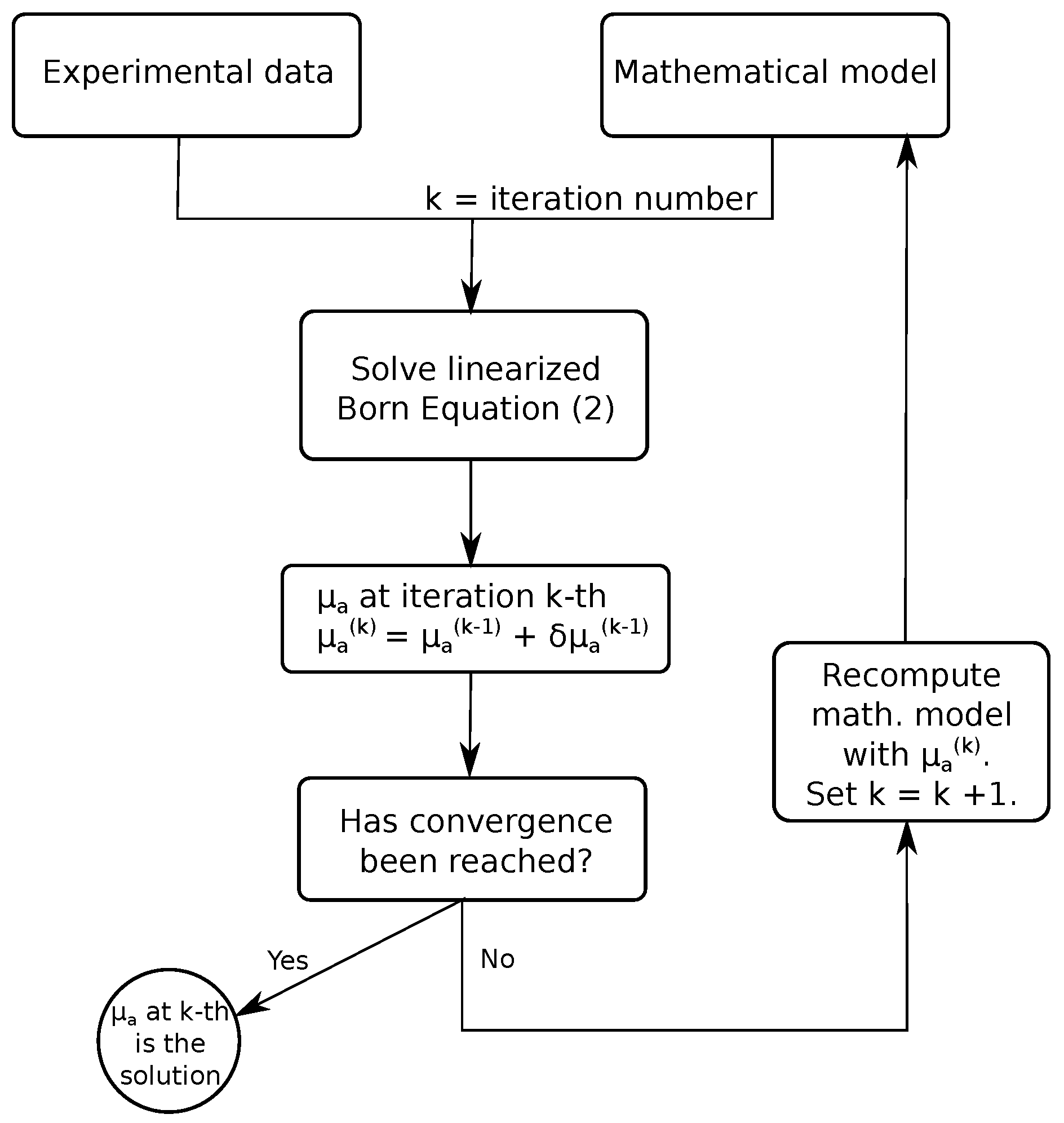
where $\delta {\varphi }_{sd}={\varphi }_{sd}-{\varphi }_{sd}^{\left(k\right)}$ is the fluence rate difference at detector d when source at position s was activated; in ${\varphi }_{sd}$ the experimental factors are included. $G_d^{\left(k\right)}(\mathbf{r},t)$ indicates the value of the Green’s function at every point in the domain assuming the source is located at position d. ${\varphi }_s^{\left(k\right)}(\mathbf{r},t)$ is the fluence rate at every point in the domain for a source located at s. $\delta {\mu }_a^{\left(k\right)}\left(\mathbf{r}\right)$ is the absorption update at each iteration. The superscript indicates that absorption values obtained at iteration k were used. The reconstructed absorption will be the result of adding all $\delta {\mu }_a$ to the initial absorption estimation, that is, ${\mu }_a=\delta {\mu }_a^{\left(1\right)}+\delta {\mu }_a^{\left(2\right)}+\dots$ A simplified sketch of the reconstruction procedure is shown at Figure 1. Equation (2) can also be extended to include changes in scattering.

Equation (2) can be discretized into a full time-resolved linear system,

$$\left[\begin{array}{c}{L}_{sd}\left(t_1\right)\\ L_{sd}\left(t_2\right)\\ ⋮\\ L_{sd}\left(t_N\right)\end{array}\right]=\left[\begin{array}{cccc}{J}_{sd}(t_1,r_1)& J_{sd}(t_1,r_2)& \cdots & J_{sd}(t_1,r_M)\\ J_{sd}(t_2,r_1)& J_{sd}(t_2,r_2)& \cdots & J_{sd}(t_2,r_M)\\ ⋮\\ J_{sd}(t_N,r_1)& J_{sd}(t_N,r_2)& \cdots & J_{sd}(t_N,r_M)\end{array}\right]\left[\begin{array}{c}\delta {\mu }_a\left(r_1\right)\\ \delta {\mu }_a\left(r_2\right)\\ ⋮\\ \delta {\mu }_a\left(r_M\right)\end{array}\right],$$

(3)

where $J_{sd}(t,r)$ and $L_{sd}\left(t\right)$ are column vectors with one entry for each source-detector pair. J matrix is known as sensitivity matrix and L is the discretization of $\delta {\varphi }_{sd}\left(t\right)$. In this case the system matrix size is $(N·S·D)\times M$ where N is the number of time bins considered, S is the number of sources, D is the number of detectors and M is the number of mesh nodes. Expressing the reconstruction in terms of time has two main drawbacks: (1) the number of time bins is high (usually of a few thousands order) which makes the system very large and (2) it is necessary to simulate the distribution of photon time of flight (DTOF) for each source and detector, which is very time-consuming.

Due to previous reasons, it is better to solve the problem of Equation (2) in terms of datatypes. A datatype is a filter that is applied to the DTOF to reduce the size of the problem. For example, when a temporal window filter is applied to the DTOF, the problem is reduced to

$$\left[\begin{array}{c}{L}_{sd}\left(w_1\right)\\ L_{sd}\left(w_2\right)\\ ⋮\\ L_{sd}\left(w_W\right)\end{array}\right]=\left[\begin{array}{cccc}{J}_{sd}(w_1,r_1)& J_{sd}(w_1,r_2)& \cdots & J_{sd}(w_1,r_M)\\ J_{sd}(w_2,r_1)& J_{sd}(w_2,r_2)& \cdots & J_{sd}(w_2,r_M)\\ ⋮\\ J_{sd}(w_W,r_1)& J_{sd}(w_W,r_2)& \cdots & J_{sd}(w_W,r_M)\end{array}\right]\left[\begin{array}{c}\delta {\mu }_a\left(r_1\right)\\ \delta {\mu }_a\left(r_2\right)\\ ⋮\\ \delta {\mu }_a\left(r_M\right)\end{array}\right],$$

(4)

whose matrix size is $W·S·D\times M$, where W is the number of windows filters used. In practice, this system will be much smaller than the system of Equation (3) since only a few dozens of windows are usually needed.

The Fourier transform is also a datatype that converts the reconstruction problem to,

$$\left[\begin{array}{c}{L}_{sd}\left(f_1\right)\\ L_{sd}\left(f_2\right)\\ ⋮\\ L_{sd}\left(f_F\right)\end{array}\right]=\left[\begin{array}{cccc}{J}_{sd}(f_1,r_1)& J_{sd}(f_1,r_2)& \cdots & J_{sd}(f_1,r_M)\\ J_{sd}(f_2,r_1)& J_{sd}(f_2,r_2)& \cdots & J_{sd}(f_2,r_M)\\ ⋮\\ J_{sd}(f_F,r_1)& J_{sd}(f_F,r_2)& \cdots & J_{sd}(f_F,r_M)\end{array}\right]\left[\begin{array}{c}\delta {\mu }_a\left(r_1\right)\\ \delta {\mu }_a\left(r_2\right)\\ ⋮\\ \delta {\mu }_a\left(r_M\right)\end{array}\right],$$

(5)

where the matrix and the vector on the left hand side are complex. The matrix size is $F·S·D\times M$, where F is the number of frequency bins. It is interesting to notice that although frequency based systems use frequencies in the range of MHz, in time-resolved systems, after applying the FT, the frequencies extend to the range of GHz. As it will be shown later, frequencies of GHz order provide important information for deep inclusions.

For the following discussion, it is important to note the difference between FT- and temporal windows-based reconstruction. In the first case, the reconstruction is done directly in the frequency domain. However, in the second case, the reconstruction is performed by using temporal windows, which are proposed to be computed in the frequency domain, due to computational efficiency reasons.

2.2. A Novel Method to Compute Temporal Windows

Let us define $u\left(t\right)$ as the DTOF simulated at a detector and $w\left(t\right)$ as an arbitrary shaped temporal window. A datatype $\Gamma$ is defined as

$${\int }_0^{\infty }u\left(t\right)w\left(t\right)\mathrm{d}t=\Gamma ,$$

(6)

since $u\left(t\right)=0$ for $t<0$. If $w\left(t\right)=t^n{e}^{-pt}$ then $\Gamma$ can be calculated directly without computing $u\left(t\right)$ explicitly [30]. However, until now, no method has been published that uses a different window form without computing explicitly $u\left(t\right)$ for each time step. The approach described in this paper proposes to compute the datatypes in the frequency domain; this can be done by using the Plancherel theorem as follows:

$$\Gamma ={\int }_{-\infty }^{\infty }u\left(t\right)\overline{w\left(t\right)}\mathrm{d}t={\int }_{-\infty }^{\infty }U\left(f\right)\overline{W\left(f\right)}\mathrm{d}f,$$

(7)

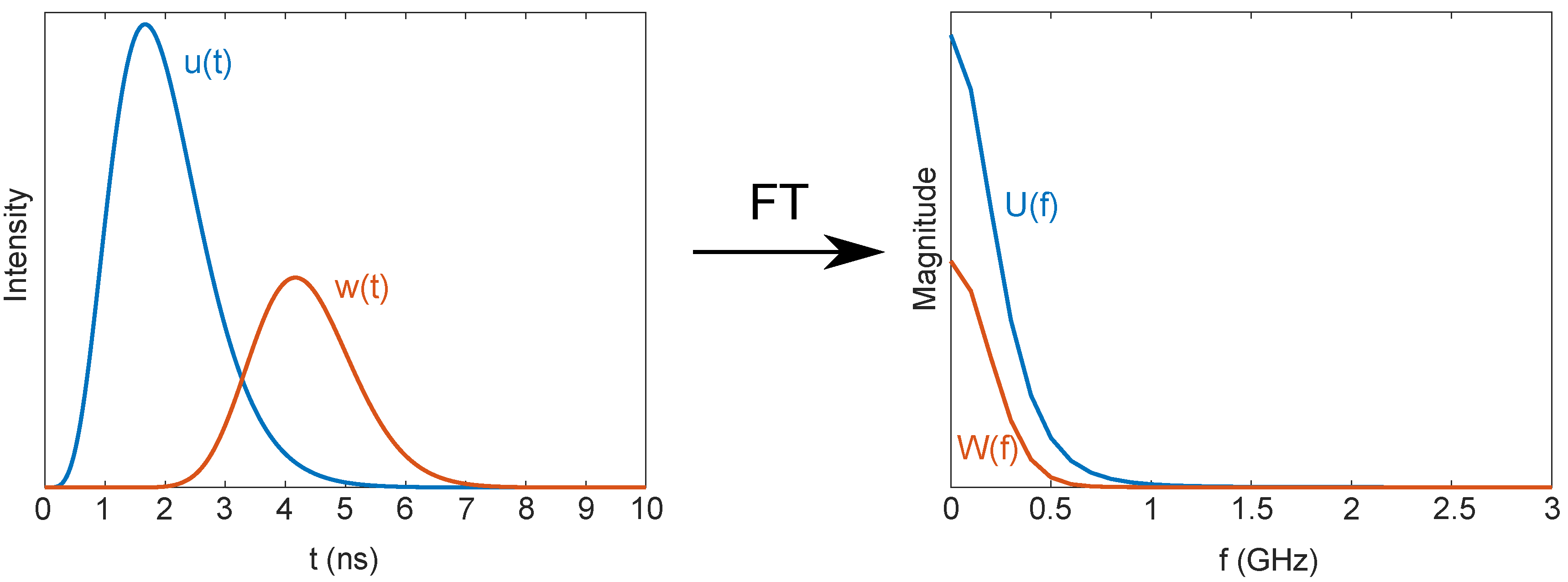
where uppercase character denotes the Fourier transform defined as $U\left(f\right)={\int }_{-\infty }^{\infty }u\left(t\right)e^{-2\pi ift}\mathrm{d}t$ (e.g., $W\left(f\right)$ is the Fourier transform of $w\left(t\right)$) and $\overline{W\left(f\right)}$ denotes the conjugate of $W\left(f\right)$. If $\overline{W\left(f\right)}$ or $U\left(f\right)$ are non-zero at a small interval of the frequency domain, the integral of Equation (7) can be approximated numerically by using few frequencies, see Figure 2. This new approach allows fast computation of a larger set of temporal windows.

To approximate $\Gamma$ using few frequencies, it is important to ensure that window spectra decay rapidly. Dispersion of the windows after applying Fourier transform can be controlled by using the uncertainty principle. This principle states that the narrower a function $g\left(t\right)$ is, the more spread its Fourier transform $G\left(f\right)$ will be. That is, if it is wanted to have a sharp window in time domain then the integral in frequency domain will be more spread around the zero frequency. Defining the dispersion of a function in time and frequency domain as

$$D_0\left(g\right)=\frac{{\int }_{-\infty }^{\infty }{t}^2{\left|g\left(t\right)\right|}^2\mathrm{d}t}{{\int }_{-\infty }^{\infty }{\left|g\left(t\right)\right|}^2\mathrm{d}t},D_0\left(G\right)=\frac{{\int }_{-\infty }^{\infty }{f}^2{\left|G\left(f\right)\right|}^2\mathrm{d}f}{{\int }_{-\infty }^{\infty }{\left|G\left(f\right)\right|}^2\mathrm{d}f}$$

(8)

the uncertainty principle states that if $g\left(t\right)$ is absolutely continuous and the functions $tg\left(t\right)$ and $g^{\prime }\left(t\right)$ are square integrable (i.e., they are in $L^2$ space) then [31]

$$D_0\left(g\right)D_0\left(G\right)\ge \frac{1}{16{\pi }^2},$$

(9)

where G is the Fourier transform of $g\left(t\right)$ and the equality holds only for the Gaussian density function centered at $t=0$.

Computational Aspects

The reported technique has to be much faster to compute than the resolution of time-dependant Diffusion Approximation equation in order to be useful in practice. In the following section, some important computational aspects related to the time complexity will be shown.

First, to compute $\varphi (\mathbf{r},t_n)$ in Equation (1), it is needed to know the previous values of $\varphi (\mathbf{r},t_{n-i})$, where $t_n$ is the n-th discrete time bin and $t_{n-i}<t_n$. This implies that to compute $\varphi (\mathbf{r},t_n)$ previously $n-1$ linear systems have to be solved. However, in the frequency resolved version of Equation (1), there is no such restriction, since the fluence rate at any frequency can be computed independently. This is the main reason why the integral of Equation (7) is faster to compute in the frequency domain. Therefore, the described technique is easily parallelizable and could be implemented in Graphics Processing Units (GPU) hardware; some labs have already implemented state-of-the-art photon propagation models using GPU technology [32,33].

Another important property is that for real functions, Fourier transform coefficients will have symmetric real part and anti-symmetric imaginary part. From this follows that only positive (or negative) frequencies must be computed and only half of the integral needs to be approximated,

$${\int }_{-\infty }^{\infty }U\left(f\right)\overline{W\left(f\right)}\mathrm{d}f=2{\int }_0^{\infty }U\left(f\right)\overline{W\left(f\right)}\mathrm{d}f\approx 2\sum _{i=0}^{N}U\left(f_i\right)\overline{W\left(f_i\right)}\Delta f,$$

(10)

where N frequencies were used in the approximation.

However, the proposed method also suffers from one limitation. When computing temporal windows with shape $w\left(t\right)=t^n{e}^{-pt}$, the linear system to solve has the form $\mathbf{A}\mathbf{x}={\mathbf{b}}^{\left(n\right)}+{\mathbf{x}}^{(n-1)}$, that is, as the order n of the window is increased, only the right part of the systems changes, but the matrix system is constant. This encourages to use, for example, LU factorization of the matrix $\mathbf{A}$ to solve all the systems quickly. However, when solving the Diffusion Approximation equation at frequency domain, the systems have the form $\mathbf{A}\left(f\right)\mathbf{x}=\mathbf{b}$ where f is the frequency. In this case, the matrix $\mathbf{A}$ needs to be factorized for each frequency, which implies an increase in the computational cost. Nevertheless, Diffusion Approximation at frequency domain is highly parallelizable because of the independence between frequencies. Therefore, unlike for model of windows $w\left(t\right)=t^n{e}^{-pt}$ the equations at each frequency-domain could be fastly solved in parallel with a GPU.

2.3. Temporal Windows

In the following subsection, most used temporal windows (standard and Mellin-Laplace moments; in this work, the words moments and windows will be used interchangeably) and proposed windows for the new method (Gaussian, Tukey and Poisson windows) are described. An analysis regarding their optimality for numerical integration is also included.

2.3.1. Standard Moments

Standard moments have been used to retrieve the optical properties of homogeneous media [34] and layered models [35]. Standard moments windows are defined as $w\left(t\right)=t^{n}H\left(t\right)$, where $n\in \mathbb{N}$ and $H\left(t\right)$ is the Heaviside step function. These types of windows can be computed fast with state-of-the-art techniques [22]. The Fourier transform of standard moment window is

$$W\left(f\right)=\frac{n!}{{\left(i2\pi f\right)}^{n+1}},$$

(11)

whose magnitude is $n!·{\left(2\pi f\right)}^{-(n+1)}$. Therefore, the standard moments in time domain are equivalent to

$${\int }_{-\infty }^{\infty }u\left(t\right)t^{n}H\left(t\right)\mathrm{d}t={\int }_0^{\infty }u\left(t\right)t^n\mathrm{d}t={\int }_{-\infty }^{\infty }U\left(f\right)\overline{{\left(i2\pi f\right)}^{-n-1}n!}\mathrm{d}f,$$

(12)

where the term $\overline{{\left(i2\pi f\right)}^{-n-1}n!}$ can be considered as a window in frequency domain. This window magnitude tends to a Dirac delta distribution as n goes to infinity, which is obvious since $t^{n}H\left(t\right)$ will approach a step function with infinity value at $t>=0$ and the only non-zero magnitude frequency in the spectrum will be the zero frequency. Therefore, the higher the order, the smaller the frequency range covered by the windows.

If the standard moments are centralized by the time of flight $\langle t\rangle ={\int }_{-\infty }^{\infty }u\left(t\right)tH\left(t\right)\mathrm{d}t$ then

$$\begin{array}{ll}{\int }_{-\infty }^{\infty }u\left(t\right){(t-\langle t\rangle )}^{n}H\left(t\right)\mathrm{d}t& ={\int }_0^{\infty }u\left(t\right){(t-\langle t\rangle )}^n\mathrm{d}t\\ & ={\int }_0^{\infty }u\left(t\right){\displaystyle \sum _{k=0}^n}\left(\genfrac{}{}{0pt}{}{n}{k}\right){\left(-1\right)}^{n-k}{t}^k{\langle t\rangle }^{n-k}\mathrm{d}t\\ & ={\displaystyle \sum _{k=0}^n}\left(\genfrac{}{}{0pt}{}{n}{k}\right){\left(-1\right)}^{n-k}{\langle t\rangle }^{n-k}{\int }_0^{\infty }u\left(t\right)t^k\mathrm{d}t,\end{array}$$

(13)

which is a weighted sum of standard moments. Now, we introduce the state-of-the-art windows known as Mellin-Laplace moments.

2.3.2. Mellin-Laplace Moments

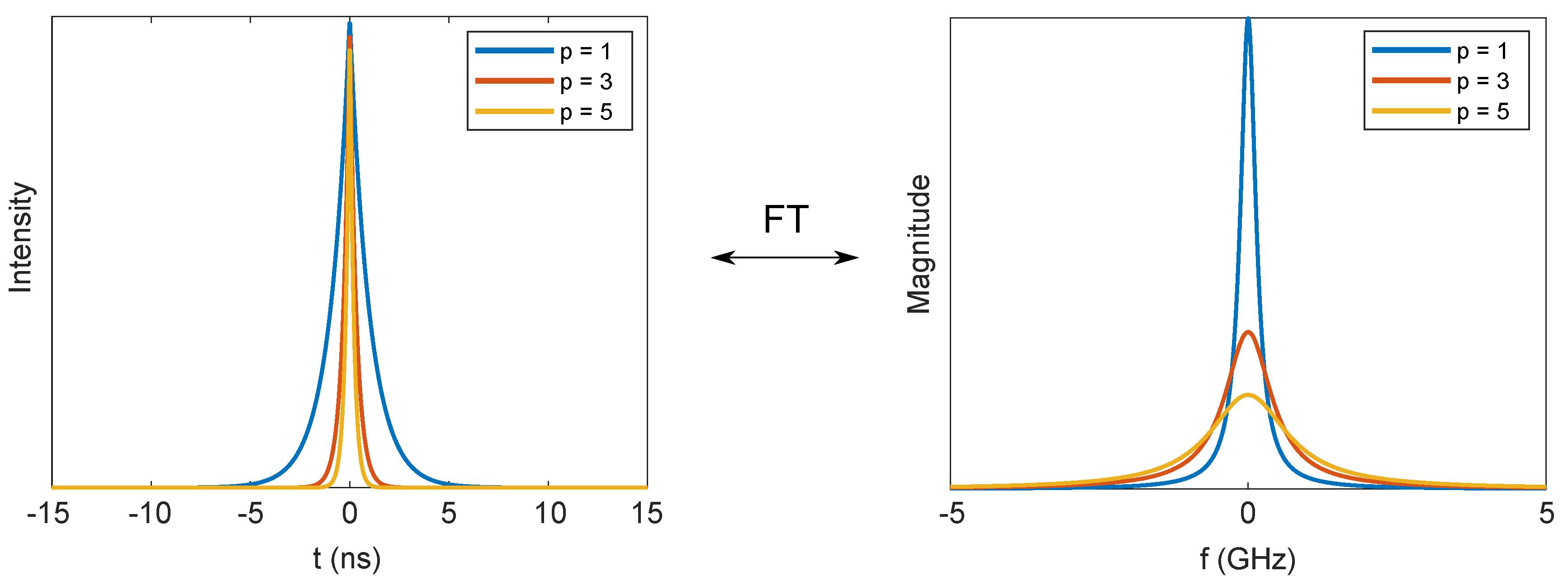
Mellin-Laplace windows are defined as $w\left(t\right)=t^n{e}^{-pt}H\left(t\right)$ where $p>0$ and $n\in \mathbb{N}$. These windows can also be computed fast [21]. Their Fourier transform is given by

$$W\left(f\right)=\frac{n!}{{(p+i2\pi f)}^{n+1}}.$$

(14)

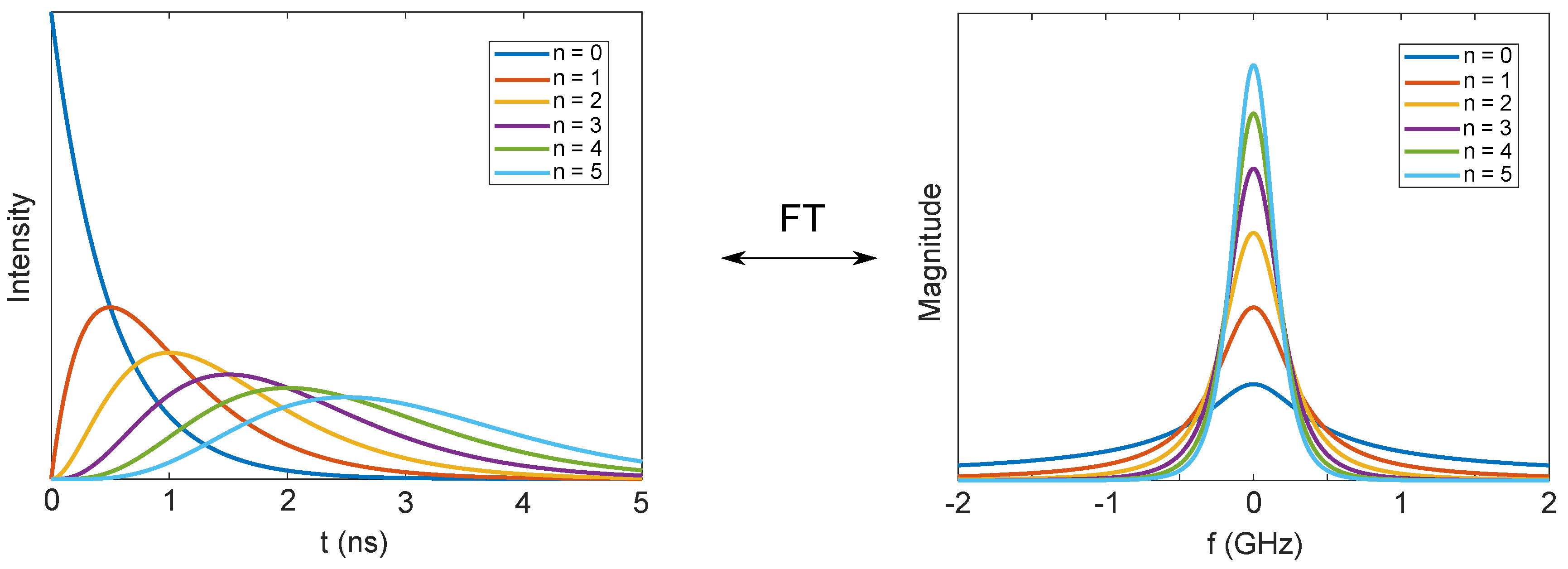
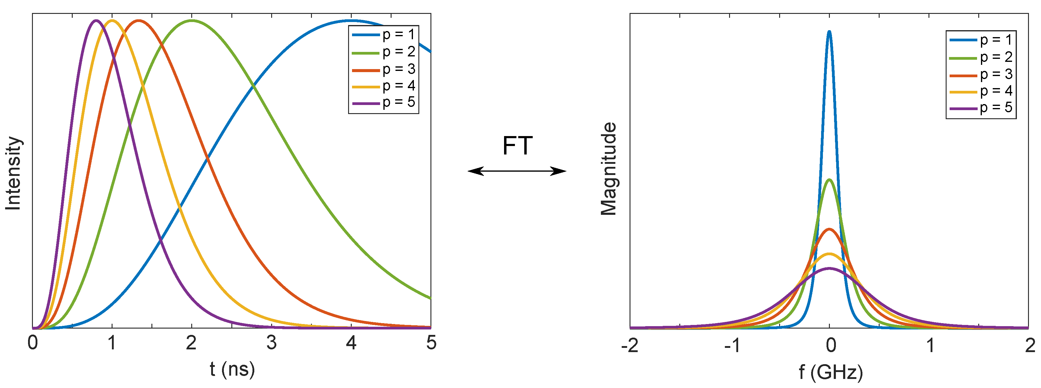
In Figure 3 and Figure 4, the windows for different n orders and p values are shown. The higher the Mellin-Laplace order n the narrower the window magnitude will be in frequency domain. As expected from the uncertainty principle, the higher the p value the more spread the window will be in frequency domain.

Zero order Mellin-Laplace datatypes are Laplace transforms for different p values. Recently, an optical system was proposed [36], which computes Laplace datatypes without the need of measuring the complete DTOF. The system described by Hasnain et al. is quite interesting, since it is much faster than typical time-resolved systems. Nevertheless, Laplace datatypes have poor temporal selectivity (they cover a broad range of time) and are highly correlated, which does not make them the best candidates in terms of tomography capabilities.

2.3.3. Generalized Gaussian Window

The Gaussian function and its Fourier transform are

$$w\left(t\right)=e^{-t^2/\left(2{\sigma }^2\right)}⟷W\left(f\right)=\sigma \sqrt{2\pi }{e}^{-2{\sigma }^2{\pi }^2{f}^2}.$$

(15)

As expected from the uncertainty principle, the higher $\sigma$, the more spread the window at time domain will be and, therefore, the narrower it will be in the frequency domain, see Figure 5. Note that the centralized Gaussian windows gives the lower bound of the uncertainty principle.

The Laplacian or exponential window (see Figure 6) are defined as

$$w\left(t\right)=exp(-p|t\left|\right)⟷W\left(f\right)=\frac{2p}{p^2+{\left(2\pi f\right)}^2},$$

(16)

where p is a parameter.

Both Gaussian and Laplacian windows can be described by the generalized Gaussian window (also known as the generalized normal window),

$$w\left(t\right)=\frac{\beta }{2\sigma \Gamma (1/\beta )}{e}^{-{\left(\right|t|/\sigma )}^{\beta }}⟷W\left(f\right)={\Gamma }^{-1}\left(\frac{1}{\beta }\right)\sum _{n=0}^{\infty }\frac{{(-1)}^n{\pi }^{2n}{f}^{2n}}{\left(2n\right)!}{\sigma }^{2n}\Gamma \left(\frac{2n+1}{\beta }\right).$$

(17)

where $\beta$ is a free parameter and $\Gamma$ is the gamma function. If $\beta =2$ the function is Gaussian and if $\beta =1$ is Laplacian. As $\beta \to \infty$ the window converges to a square window.

2.3.4. Tukey Window

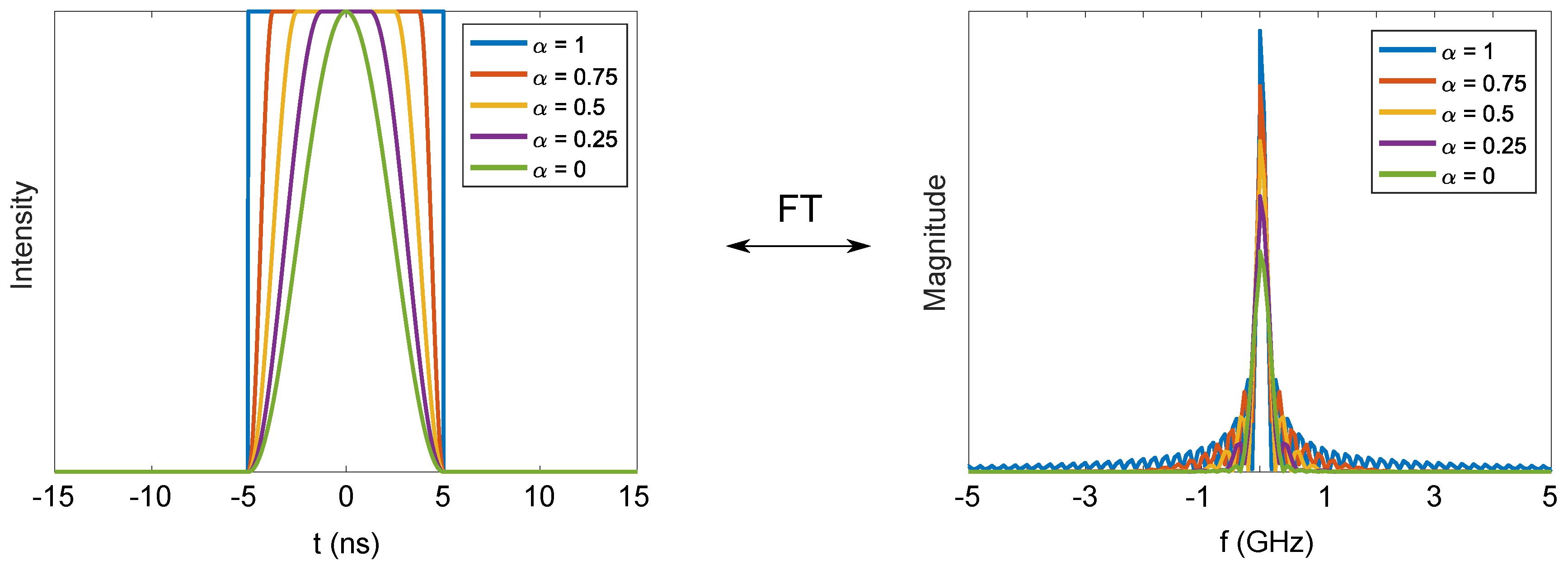
The centralized Tukey window [37] is defined as

$$w\left(t\right)=\{\begin{array}{ll}1,& 0\le \left|t\right|\le \alpha t^{*}\\ 0.5\left[1+cos\left(\pi \frac{t-\mathrm{sign}\left(t\right)\alpha t^{*}}{\mathrm{sign}\left(t\right)\left(t^{*}-\alpha t^{*}\right)}\right)\right],& \alpha t^{*}\le \left|t\right|\le t^{*},\\ 0,& \mathrm{elsewhere},\end{array}$$

(18)

where $t^{*}$ is the limit of the window and $0\le \alpha \le 1$ parameter controls the smoothness of the window.

If $\alpha =1$ the Tukey window is rectangular and its Fourier transform is defined as

$$w\left(t\right)=\mathrm{rect}(t/\tau )⟷W\left(f\right)=\tau \mathrm{sinc}\left(\pi f\tau \right).$$

(19)

These windows have a high selectivity of photon arrival time. The spectrum magnitude of rectangular function ($\alpha =1$) is a $\mathrm{sinc}$ function with infinite oscillations, which can make difficult to integrate them numerically. Nevertheless, as the $\alpha$ value decreases, the oscillations at high frequencies disappear without losing much temporal selectivity. Note that before presenting this novel computation method, rectangular windows were only used for functional near-infrared spectroscopy analysis [38] but not for tomography since they could not be calculated without computing the full time-resolved curve.

2.3.5. Trade-Off between Temporal Selectivity and Computation Complexity

An optimal temporal window is the one that is easy to compute (it has few oscillations and small dispersion at frequency domain) and at the same time its temporal selectivity is good enough. For some windows, optimality can be described by $D_0^{*}=D_0\left(g\right)D_0\left(G\right)$ (see Section 2.2). The $D_0^{*}$ of a window quantifies the trade-off between the temporal selectivity and easiness to compute as expressed by uncertainty principle. The lower the value $D_0^{*}$ is for a given window, the better the window temporal selectivity will be and the less frequencies will be needed to perform the numerical integration.

In

Table 1. $D_0^{*}$ for each analyzed window. Standard moments and Tukey windows are not $L^2$ integrable. See Appendix A for calculations.

Window	${\mathit{D}}_0^{*}$
Mellin-Laplace	$\frac{1}{16{\pi }^2}\frac{(2n+2)!}{\left(2n\right)!}\left(\frac{2n}{2n-1}-1\right),(n\ge 1)$
Gaussian	$1/\left(16{\pi }^2\right)$
Exponential	$1/\left(8{\pi }^2\right)$

, the main optimality results are summarized.

The Gaussian is the window that has the lowest $D_0^{*}$ value; this was expected from the uncertainty principle theorem and this is what makes the Gaussian window one of the most promising windows. The exponential window has a twice bigger value compared to the Gaussian window; this means that the numerical integral could be a bit more difficult to compute but it is still a good candidate. Mellin-Laplace windows will increase its $D_0^{*}$ value almost linearly for increasing orders although it is independent of p value. Expression $D_0^{*}$ is not in $L^2$ space for Tukey windows, nevertheless from Figure 7 it is evident that for some $\alpha$ values is still feasible to perform numerical integration at frequency domain. Standard moments are neither $L^2$ integrable. Those moments were analyzed in detail in [39,40] and one of the conclusions that was reached is that standard moments high orders are only profitable when more than ${10}^8$ photons are detected. Moreover, since by nature they are highly correlated (see Figure 8a) they will not be considered in this work.

A point that should also be taken into account is the shift theorem of the Fourier transform. It states that given a function $g\left(t\right)$, if this function is shifted an amount of $t_0$, then its Fourier transform is

$$G_{t-t_0}\left(f\right)=G\left(f\right)e^{-i2\pi f{t}_0},$$

(20)

where $G_{t-t_0}\left(f\right)$ indicates the Fourier transform of shifted function $g(t-t_0)=g\left(t\right)\ast \delta (t-t_0)$ and the complex exponential does not affect the spectral magnitude since $|e^{-i2\pi f{t}_0}|=1$ but it affects the phase. This theorem implies that as temporal windows are shifted to later times, more oscillations will appear. However, in practice this phenomenon did not prevent us to perform the numerical integration accurately.

The new method to compute temporal windows is also useful for windows with the form $w\left(t\right)=t^n{e}^{-pt}$, such as Mellin-Laplace or standard moments. Both of these moments suffer from an important handicap if traditional computation methods are used: in order to compute the n-th order window then all the previous orders, $1,...,n-1$, must be computed (in the case of Mellin-Laplace if p parameter is modified then all orders must be computed again). These problem can be critical in the case of Mellin-Laplace since as the order of the moments increase, the window temporal selectivity decreases (see Figure 3(left)). If it is wanted to have better sensitivity to later photons (i.e., photons that probabilistically have go deeper into the tissue) then higher p values must be used. There are two ways of doing it: the first option is to use the same p value for all windows; but the main drawback is that many orders will have to be calculated, since a higher p value shifts windows average time-of-flight to earlier photons (see Figure 4). The second option implies to use windows with different p values (e.g., a low p value for early windows and high p values for late windows) which is not computationally efficient since if the p value is changed then all orders up to n will have to be computed again as explained before. Nevertheless, the new approach presented in this paper does not suffer from these bottlenecks since Mellin-Laplace moments can be computed for each p and n value independently (same for n order in the case of standard moments). Therefore, one of the advantages of the presented method is not only that new windows can be computed but also that Mellin-Laplace windows for different p values can be computed more efficiently.

2.4. Noise Correlations

Since DTOF signals are transformed to windows space, the noise will also suffer changes. In this part, noise transformations and correlations are analysed to understand noise influence.

The DTOF signal measured by a detector is theoretically described as

$$u\left(t\right)=x\left(t\right)+\epsilon \left(x\right(t\left)\right),$$

(21)

where $x\left(t\right)$ is the noiseless signal and $\epsilon$ is the noisy term which depends on $x\left(t\right)$ magnitude, uncorrelated (that is, $\mathrm{Cov}(\epsilon \left(x\left(t\right)\right),\epsilon \left(x\left(t^{\prime }\right)\right))=0$ for $t\ne t^{\prime }$) and follows a Poisson distribution. Applying the Fourier transform to $u\left(t\right)$ yields,

$$\begin{array}{cc}\hfill U\left(f\right)& =X\left(f\right)+{\rm Y}\left(f\right)\hfill \\ \hfill & ={\int }_{-\infty }^{\infty }x\left(t\right)e^{-i2\pi ft}\mathrm{d}t+{\int }_{-\infty }^{\infty }\epsilon \left(x\left(t\right)\right)e^{-i2\pi ft}\mathrm{d}t,\hfill \end{array}$$

(22)

where the second term in the right part is the noisy contribution and $U\left(f\right)$ can be considered a random variable. As stated before, in time domain, the noise at each time bin is independent, however after applying the Fourier transform this property does not hold anymore. For example, the covariance between two different frequencies is,

$$\begin{array}{ll}\hfill E\left[U\left(f_1\right)·\overline{U\left(f_2\right)}\right]-E\left[U\left(f_1\right)\right]·E\left[\overline{U\left(f_2\right)}\right]& =E\left[{\int }_{-\infty }^{\infty }u\left(t\right)e^{-i2\pi f_{1}t}\mathrm{d}t·\overline{{\int }_{-\infty }^{\infty }u\left(t\right)e^{-i2\pi f_{2}t}\mathrm{d}t}\right]\\ & -E\left[{\int }_{-\infty }^{\infty }u\left(t\right)e^{-i2\pi f_{1}t}\mathrm{d}t\right]·E\left[\overline{{\int }_{-\infty }^{\infty }u\left(t\right)e^{-i2\pi f_{2}t}\mathrm{d}t}\right]\\ & ={\int }_{-\infty }^{\infty }{\int }_{-\infty }^{\infty }\left(E\left[u\left(t\right)·u\left(t^{\prime }\right)\right]-E\left[u\left(t\right)\right]·E\left[u\left(t^{\prime }\right)\right]\right)e^{-i2\pi f_{1}t}{e}^{i2\pi f_2{t}^{\prime }}\mathrm{d}t\mathrm{d}{t}^{\prime }\\ \hfill (\mathrm{Due}\mathrm{to}\mathrm{TR}\mathrm{signal}\mathrm{noise}\mathrm{independence})& ={\int }_{-\infty }^{\infty }E\left[u\left(t\right)\right]e^{-i2\pi (f_1-f_2)t}\mathrm{d}t\\ \hfill (E\left[u\left(t\right)\right]=x\left(t\right),\mathrm{due}\mathrm{to}\mathrm{shot}/\mathrm{Poisson}\mathrm{noise})& ={\int }_{-\infty }^{\infty }x\left(t\right)e^{-i2\pi (f_1-f_2)t}\mathrm{d}t\\ & =X(f_1-f_2),\hfill \end{array}$$

(23)

so the covariance of Fourier transform signal at two different frequencies is equal to the Fourier coefficient of the noiseless signal at frequency $f_1-f_2$. See Appendix B for an alternative proof.

From this result, the covariance between any temporal window datatypes can be determined. Let us define a window datatype shifted $k{t}_0$ in time as,

$$M_{k,t_0}={\int }_0^{\infty }u\left(t\right)w(t-k{t}_0)\mathrm{d}t={\int }_{-\infty }^{\infty }U\left(f\right)\overline{W\left(f\right)}{e}^{i2\pi fk{t}_0}\mathrm{d}f,$$

(24)

where $t_0$ is the shift unit length and k is the number of shifts steps that are taken. Then, the covariance between shifted window datatypes is,

$$\begin{array}{ll}\hfill \mathrm{Cov}(M_k,M_l)& =E\left[{\int }_{-\infty }^{\infty }U\left(f\right)\overline{W\left(f\right)}{e}^{i2\pi fk{t}_0}\mathrm{d}f·\overline{{\int }_{-\infty }^{\infty }U\left(f\right)\overline{W\left(f\right)}{e}^{i2\pi fl{t}_0}\mathrm{d}f}\right]\\ & -E\left[{\int }_{-\infty }^{\infty }U\left(f\right)\overline{W\left(f\right)}{e}^{i2\pi fk{t}_0}\mathrm{d}f\right]·E\left[\overline{{\int }_{-\infty }^{\infty }U\left(f\right)\overline{W\left(f\right)}{e}^{i2\pi fl{t}_0}\mathrm{d}f}\right]\\ & ={\int }_{-\infty }^{\infty }{\int }_{-\infty }^{\infty }\left(E\left[U\left(f\right)·\overline{U\left(f^{\prime }\right)}\right]-E\left[U\left(f\right)\right]·E\left[\overline{U\left(f^{\prime }\right)}\right]\right)\overline{W\left(f\right)}{e}^{i2\pi fk{t}_0}W\left(f^{\prime }\right)e^{-i2\pi f^{\prime }l{t}_0}\mathrm{d}f\mathrm{d}{f}^{\prime }\\ & ={\int }_{-\infty }^{\infty }{\int }_{-\infty }^{\infty }X(f-f^{\prime })\overline{W\left(f\right)}W\left(f^{\prime }\right)e^{i2\pi (k{t}_{0}f-l{t}_0{f}^{\prime })}\mathrm{d}f\mathrm{d}{f}^{\prime }.\end{array}$$

(25)

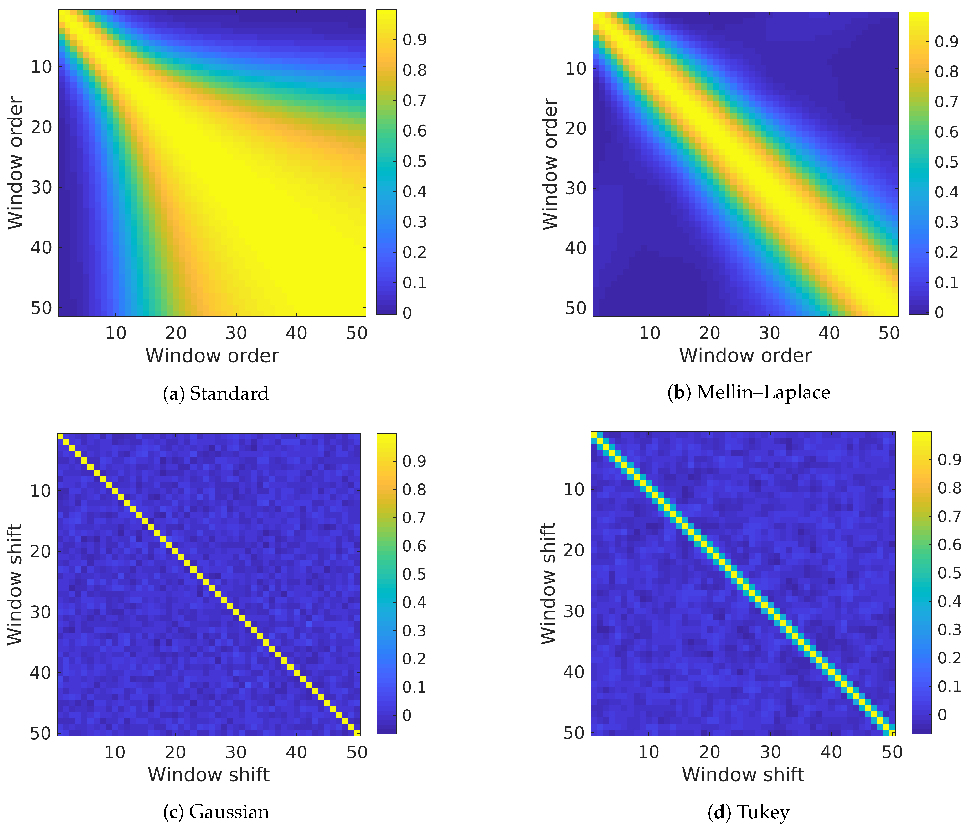
From Equation (25), the covariance and correlation matrices of any window can be obtained. Note that for standard (and Mellin-Laplace) moments the shift is already fixed by n (and p) value. In Figure 8, an example of the typical correlation matrices of standard, Mellin-Laplace, Gaussian and Tukey windows are shown. It is evident that, the greater the order of the standard moment, the more correlated it is with the rest of moments, see Figure 8a to get an intuitive idea. In the case of Mellin-Laplace window for a fixed p value, as the order n increases, its get more and more correlated with neighbour windows, see Figure 8b, although not as much as standard moments. However, for Gaussian and Tukey windows, the correlation can be minimized by separating them far enough; in the example given the Gaussian windows are not correlated with any other windows, because the windows did not overlap. The same thing could have been done with Tukey windows.

In time-domain reconstruction, the heteroscedasticity [41] is present in the noise, that is, the noise at each time bin has different variance but they are not correlated with each other (this is due to photon noise physics). After applying overlapping windows, such as Mellin-Laplace or Fourier transform, non-zero covariance values will appear. Therefore, in these cases, Least Squares (LS) will not be a Best Linear Unbiased Estimator (BLUE) anymore. Nevertheless, Generalized Least Squares (GLS) (also known as Aitken’s estimator) can be used instead, which is also a BLUE [41]. In theory, LS and GLS will reach the same solution for different noise realizations, however since for GLS the inverse of covariance matrix must be computed, some problems could arise if it is ill-posed. So, noise correlations should be avoided whenever possible.

2.5. Numerical Simulations

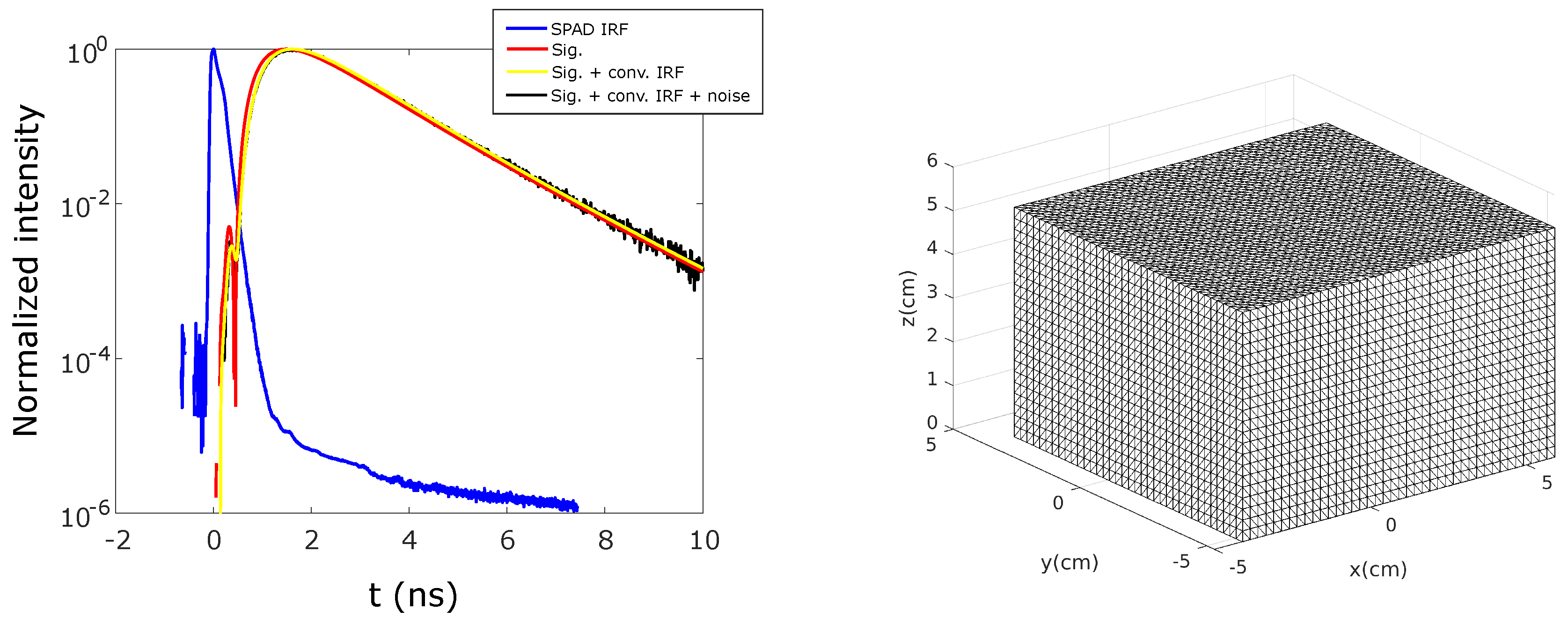
To analyze the reconstruction improvements that could be obtained with the decorrelated windows, some numerical simulations were performed. The used computational phantom was a three-dimensional volume with a spherical inclusion at different depths. This phantom can be consider as an approximation to functional near-infrared spectroscopy experiments where the inclusion represents the activation in the cortex. The computational phantom had a size of $9\times 9\times 5{\mathrm{cm}}^3$. Numerical simulations were performed in a reflectance geometry by solving the time-domain Diffusion Approximation up to 10 ns; the boundary conditions were implemented as described in [42]. To generate the synthetic measurements the domain was discretized using around 32 and 172 thousand nodes and elements respectively, see Figure 9(right). For the reconstruction, a coarser mesh was used (9 and 48 thousand nodes and elements respectively) in order to avoid inverse crime phenomenon. Each simulated curve contained up to $2\times {10}^5$ photons, were convoluted with the instrumental response function of a single photon avalanche diode detector (SPAD, FWHM ≈ 160 ps) and corrupted by Poisson noise, see Figure 9(left).

In this work, only absorption inhomogeneities were considered, although it can be easily extended to scattering inhomogeneities. Background absorption was set to ${\mu }_a=0.018{\mathrm{cm}}^{-1}$ and the reduced scattering was ${\mu }_s^{\prime }=14.7{\mathrm{cm}}^{-1}$ over all the domain. An inclusion of $0.5\mathrm{cm}$ radius was included whose optical properties were ${\mu }_a=0.337{\mathrm{cm}}^{-1}$ and ${\mu }_s^{\prime }=14.7{\mathrm{cm}}^{-1}$ (these values were taken from the experiment performed at [43] using $550\mathrm{nm}$ wavelength light and are of similar order as found at several types of human tissue).

The setup of source and detectors was moved along the top boundary to scan the phantom at multiple positions. The distance between the source and detectors was 3 cm at orthogonal directions, see Figure 10. The scan of the computational phantom with the inclusion was done at 30 different source positions (6 shifts in x-direction separated by 0.75 cm and 5 shifts in y-direction separated by 0.75 cm). The inclusions were set from 1 to 4 cm depth.

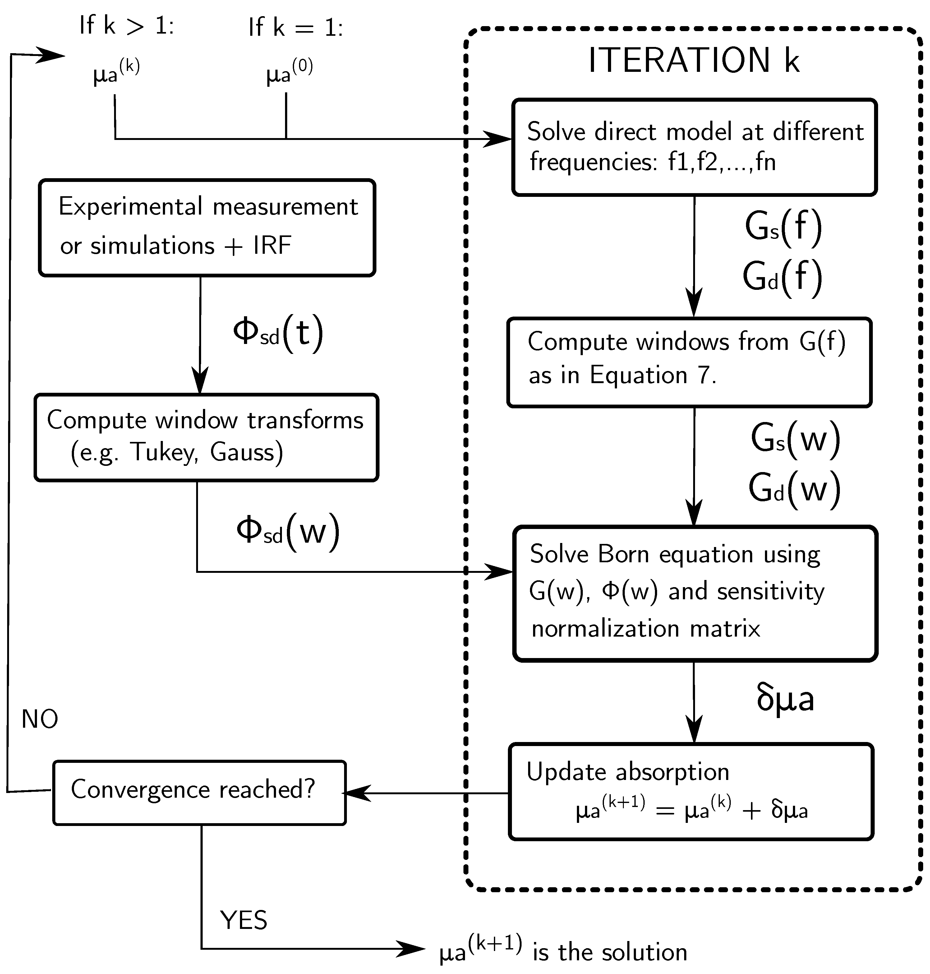
During the reconstruction, to avoid large sensitivities in the surface nodes the sensitivity of each node was normalized by a diagonal weight matrix with values proportional to nodes depth. A flowchart of the used algorithm is shown at Figure 11. Simulations and reconstructions were done using a laptop with an Intel Core i7 processor and $4\mathrm{GB}$ RAM.

2.6. Quantitative Evaluation Metrics

Three different evaluation metrics (localization error, average contrast and relative recovered volume) were used to measure the reconstructions quality from different points of view.

Localization error is defined as Euclidean distance between the center of mass of simulated inclusion ${\mathbf{x}}_s$ and the center of mass of the reconstructed inclusion ${\mathbf{x}}_r$. If the reconstructed optical properties are identical to the truth, the localization error is zero. The recovered inclusion is determined by selecting the reconstructed absorption changes that are greater than a given threshold defined later.

$$\mathrm{Localization}\mathrm{error}=\parallel {\mathbf{x}}_s-{\mathbf{x}}_r{\parallel }_2.$$

(26)

The average contrast evaluation metric is based on the mean value of the region of interest (i.e., inclusion volume):

$$\mathrm{Average}\mathrm{contrast}=\frac{{\sum }_{i\in N_r}{\mu }_i}{|N_r|\widehat{\mu }}$$

(27)

where ${\mu }_i$ denotes the reconstructed absorption at node i, $N_r$ represents the set of nodes at the region of interest, $|N_r|$ denotes the number of nodes within the set and $\widehat{\mu }$ is the truth values of absorption at the region of interest. If the reconstructed absorption is identical to the truth, the average contrast value is one.

The last evaluation metric is the relative reconstructed volume ($V_{RRV}$) which is defined as

$$V_{RRV}=V_r/V_s\times 100\%$$

(28)

where $V_r$ and $V_s$ are the volume of the reconstructed inclusion and simulated case respectively. The volume of the reconstructed inclusion, $V_r$, is computed by thresholding the recovered absorption changes and computing the volume of those elements. If the reconstructed absorption is identical to the truth, the relative reconstructed volume is one.

3. Results and Discussion

In this section, the simulations results are given in order to analyze the performance of tomography algorithms based on temporal windows and Fourier transform datatypes. Subsequently, different perspectives of the same problem are given and results are discussed.

3.1. Comparing State-of-the-Art Windows with Tukey and Gaussian Windows

The purpose of the first simulations is to check whether Tukey or Gaussian windows improve the reconstruction in depth compared to $w\left(t\right)=t^n{e}^{-pt}$ state-of-the-art windows.

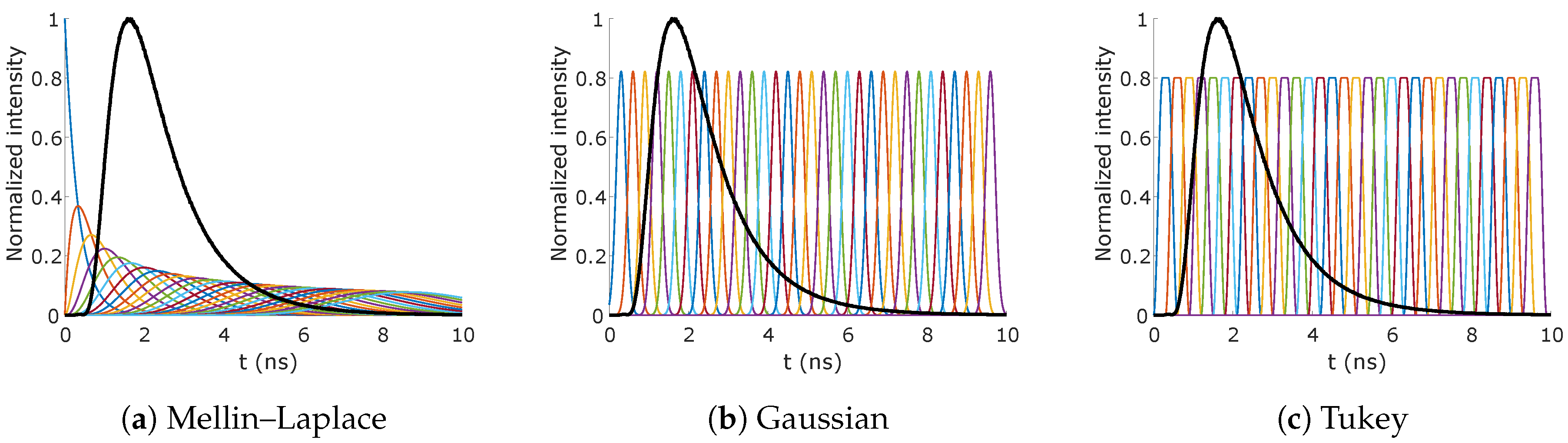
For the Mellin–Laplace reconstruction $p=3$ and the first 35 moments were used (Figure 12a). For Gaussian windows, the value of $\sigma$ was set to $0.3$ and their centers were located from $0.3$ to $9.6$ ns in steps of $0.3$ ns (32 windows in total, Figure 12b). For the Tukey windows, the same centers were used and the parameters were set to $\alpha =0.25$ and $t^{*}=0.3$ ns (Figure 12c). The given parameters were selected so that in all cases the windows totally covered the simulated signal and the number of windows were similar (35 for Mellin–Laplace and 32 for Tukey and Gaussian). The computed frequencies ranged from 0 to 2 GHz in steps of 200 MHz.

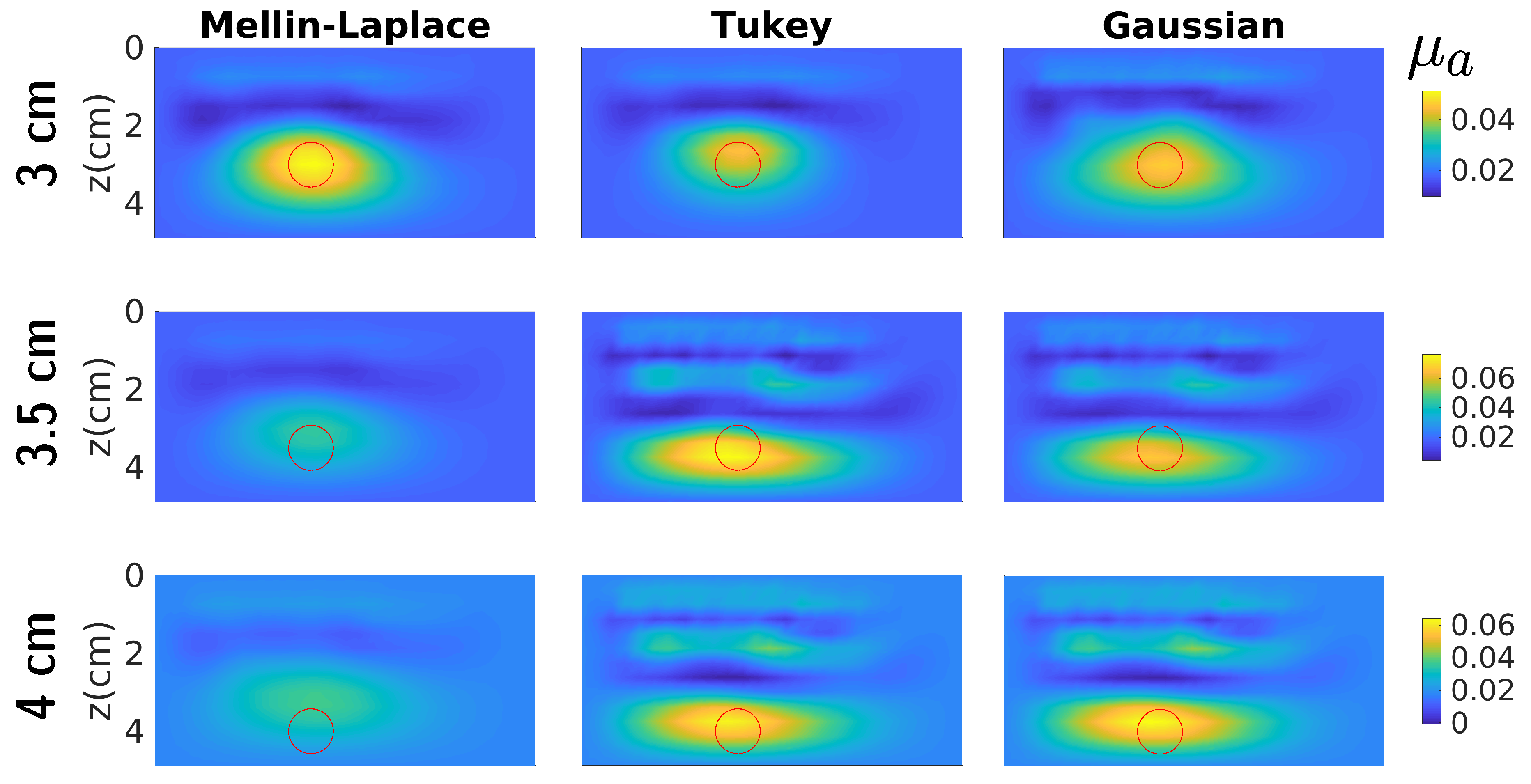
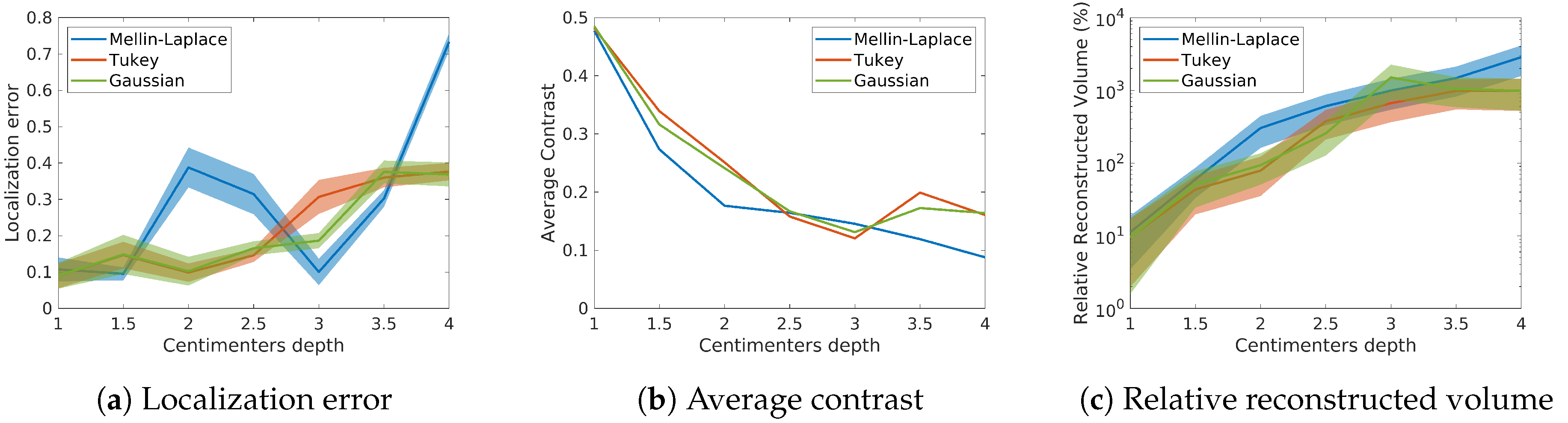
The Figure 13 shows reconstruction using Melin-Laplace, Tukey and Gaussian temporal windows for inclusions that ranged from 1 to 2.5 cm deep (in steps of 0.5 cm). In Figure 14, the reconstructions for inclusions from $3\mathrm{cm}$ to $4\mathrm{cm}$ deep are given. In Figure 15, the evaluation metrics results are shown for each method. Significant differences are seen for inclusions shallower than $2.5\mathrm{cm}$ not just in terms of localization accuracy but also regarding absorption quantification. Localization error for Mellin-Laplace windows is around $0.4\mathrm{cm}$ for the inclusion located at $2\mathrm{cm}$ depth. However, for the novel windows the maximum localization error is $0.2\mathrm{cm}$. Moreover, the absorption quantification is constantly underestimated by Mellin-Laplace windows, see how average contrast metric decreases exponentially and the contrast of Tukey and Gaussian windows is always greater than Mellin-Laplace windows in the range of 1 to $2.5\mathrm{cm}$ depth. For inclusions deeper than $3\mathrm{cm}$ Mellin–Laplace windows reconstruction is significantly worse in terms of absorption quantification. Also note that the localization error for Mellin-Laplace windows is much larger for the inclusion $4\mathrm{cm}$ deep; these results are in agreement with [44] which shows the same problem beyond $2\mathrm{cm}$ depth. Moreover, the relative reconstructed volume also increases due to the fact that Mellin-Laplace loses the inclusion localization and absorption quantification, and therefore, it tries to compensate it by reconstructing higher volume inclusions, see for example the inclusion at depth $2.5\mathrm{cm}$. This phenomenon occurs due to the diffusion of photons inside the medium. In contrast, the results also show that Tukey and Gaussian windows give very similar reconstructions and their localization error is always less than $0.4\mathrm{cm}$.

The fact that proposed windows outperform Mellin-Laplace state-of-the-art windows for deep inclusions can be explained by the theoretical analysis shown in the previous sections. First, Mellin–Laplace windows have a poor late-arrival photon selectivity and windows are highly correlated. This implies that each Mellin–Laplace window has very little new information by itself. As the order of the Mellin–Laplace window increases the new information that it carries decreases. That implies that a huge amount of window should be used to include all the available information in the DTOFs. This evidence demonstrate the superior performance of Gaussian and Tukey window compared to Mellin–Laplace because of the better photon time arrival selectivity and less noise correlation.

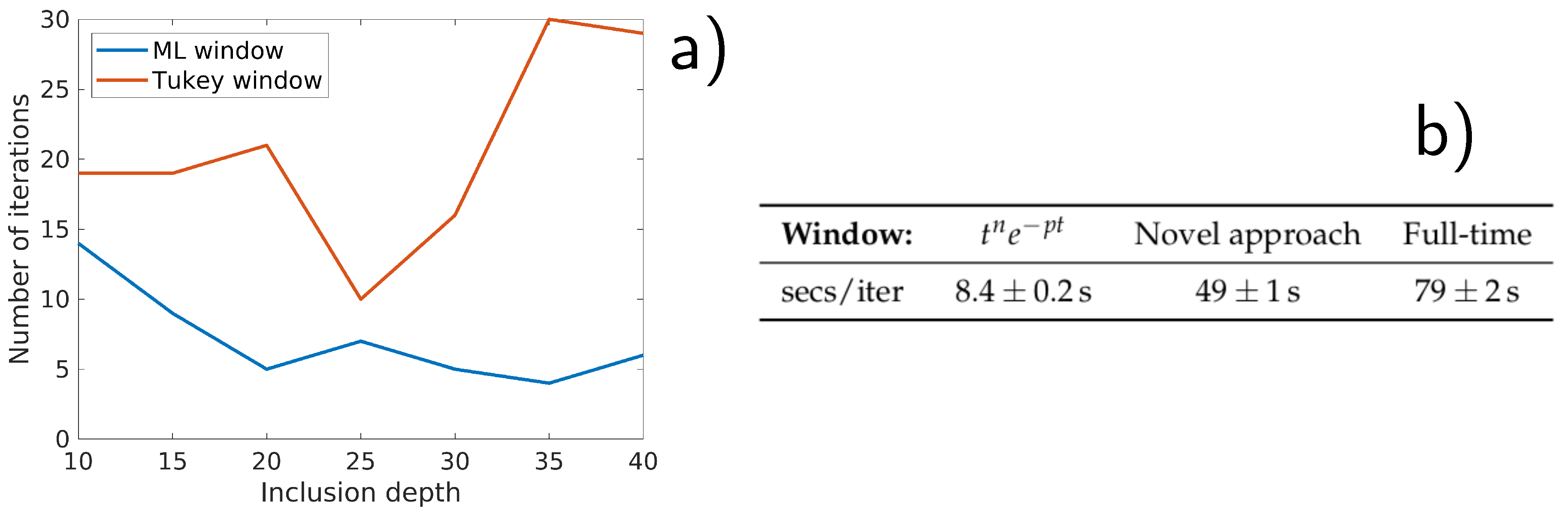
Regarding the computation time of the reconstructions, in Figure 16b the number of seconds per iteration is given for each method. To compute windows with form $t^n{e}^{-pt}$ is much faster than the proposed approach and full-time reconstruction. Specifically, $t^n{e}^{-pt}$ windows are around six times faster to compute than the proposed approach because $LU$ factorization can be applied. However, for the proposed method factorization is not efficient since the matrix changes at each frequency. Full–time resolved approach is $9.5$ times slower than $t^n{e}^{-pt}$ windows and around $1.6$ slower than the proposed approach. These results shows the trade-off of the proposed method: more information in depth is obtained but computation time is larger than $t^n{e}^{-pt}$ windows. However, it should also be taken into account that novel method approach is highly parallelizable, that is, the Diffusion Approximation equation can be solve independently for each frequency. Note that this property does not hold for the direct computation of $t^n{e}^{-pt}$ windows [22] and full–time approach. Therefore, the computation time of novel approach should considerably improve with GPU usage due to its intrinsic parallelizable nature. In Figure 16a, the number of computed iterations until convergence is given. Convergence was reached when relative difference $\delta {\mu }_a/{\mu }_a^{\left(k\right)}<5\times {10}^{-3}$. It can be seen that Mellin–Laplace windows converge faster mainly because it underestimates absorption quantification.

As explained before, the simulated DTOFs were convolved with an SPAD IRF and corrupted with photon noise. These DTOFs were deconvoluted with a Wiener filter before performing the reconstruction. In some papers, such as [21], a different approach is proposed: DTOFs from a reference medium A and objective medium B are used. The optical properties of medium A are already known because an homogeneous medium is taken as reference and it includes implicitly all the information regarding instrumental factors. The medium B is the medium to be reconstructed. Absorption of medium B can be recovered by using iteratively the linearized cross–Born equation,

$$G_{sd}^A(\mathbf{r},t)\ast M_{sd}^B(\mathbf{r},t)-M_{sd}^A(\mathbf{r},t)\ast G_{sd}^{B\left(k\right)}(\mathbf{r},t)=-M_{sd}^A(\mathbf{r},t)\ast {\int }_{\Omega }\left[G_s^{B\left(k\right)}\ast G_d^{B\left(k\right)}\right](\mathbf{r},t)\delta {\mu }_a\mathrm{d}\mathbf{r},$$

(29)

where ∗ is the convolution operator, $M_{sd}^A$ and $M_{sd}^B$ indicate the measurement obtained at reference and to be reconstructed media by detector d when source s was activated, k indicates the iteration number, $G_{sd}^A$ and $G_{sd}^{B\left(k\right)}$ is the simulated Green’s function (free of noise and instrumental factors) from source s at detector d by using the photon propagation mathematical model described in Equation (1) and $G_s^{B\left(k\right)}$ indicates the Green’s function value at every point in the domain given by the propagation model.

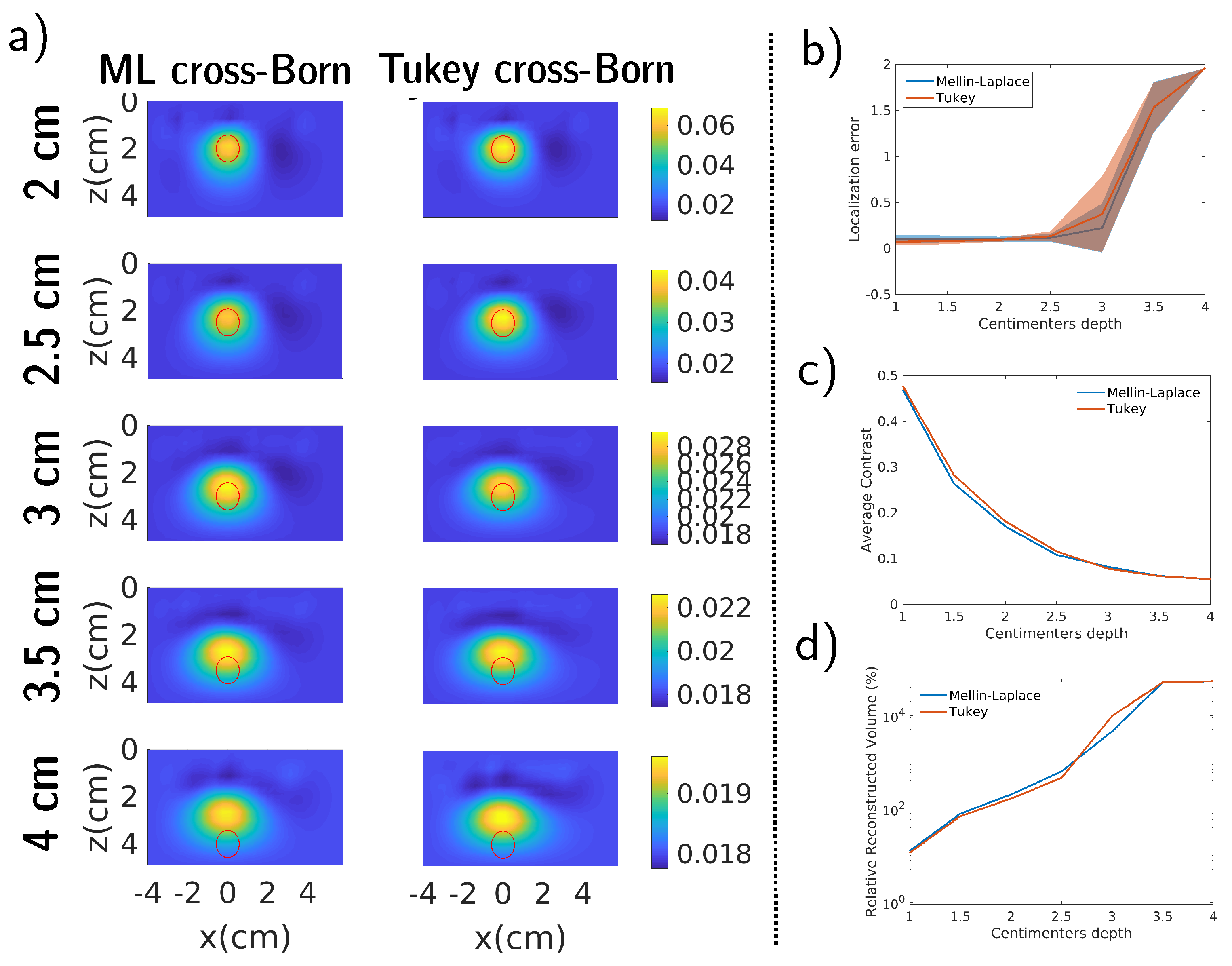
The cross–Born equation offers the ease of not having to deal with instrumental factors directly (no deconvolution of the measurements is needed). However, it also implies to convolve the data and lose some information in the process. In Figure 17a, reconstructions using Mellin–Laplace and Tukey windows with the cross–Born approach are shown. We chose Tukey windows since they give very similar results to Gaussian windows. In Figure 17b–d, the quantitative metrics for those simulations are given. Results for inclusions as deep as $3\mathrm{cm}$ are very similar to the deconvolution approach, but for inclusion deeper or equal to $3.5\mathrm{cm}$ the localisation accuracy is lost, see Figure 17b. Moreover, the contrast is lower than previous reconstructions; although, slight differences are seen between Mellin-Laplace and Tukey windows even using cross-Born equation, see Figure 17c. The relative recovered volume increases considerably for both methods (Figure 17d. These results show that when the cross–Born approach is used, some information in depth is lost for inclusions deeper than $3\mathrm{cm}$ and to take full advantage of not overlapping datatypes (e.g., Tukey or Gaussian windows), experimental data must be deconvoluted before performing a reconstruction.

From a different point of view, this theoretical analysis can also be viewed as an explanation of full time-resolved tomography limits. That is, Tukey windows-based reconstruction can be seen as an intermediate step between correlated windows-based reconstruction and full time-resolved reconstruction (i.e., reconstruction based on using each time bin as a datatype). In fact, in the last years several labs [32,33], have developed photon propagation models for Graphics Processing Units (GPU). One of the goals of using GPU is to compute the full DTOF curve and to fit it entirely as described in Equation (3). To fit the entire DTOF curve is the limiting case of very narrow Tukey windows; if windows are shrinked to time bin size it will converge to DTOF curve fitting. Therefore, some of the questions that arise from this theoretical work is, how much benefit can be obtained by using full time-resolved reconstructions? Does the computational cost of computing the full curve outweighs the gain of some information? Moreover, since the computation of decorrelated windows, such as Tukey or Gaussian, are easily parallelizable and adaptable to GPU hardware, the authors believe that this computation method is an efficient substitute to full time-resolved reconstructions.

3.2. Comparing Windows and Frequency-Based Reconstruction

One of the question that could arise now is why not to apply the Fourier transform to DTOFs signals and perform the frequency based reconstruction described at Equation (5). To answer this question, reconstructions were also performed using Fourier transform datatypes for an inclusion 3.5 cm deep with the same optical values in the previous section.

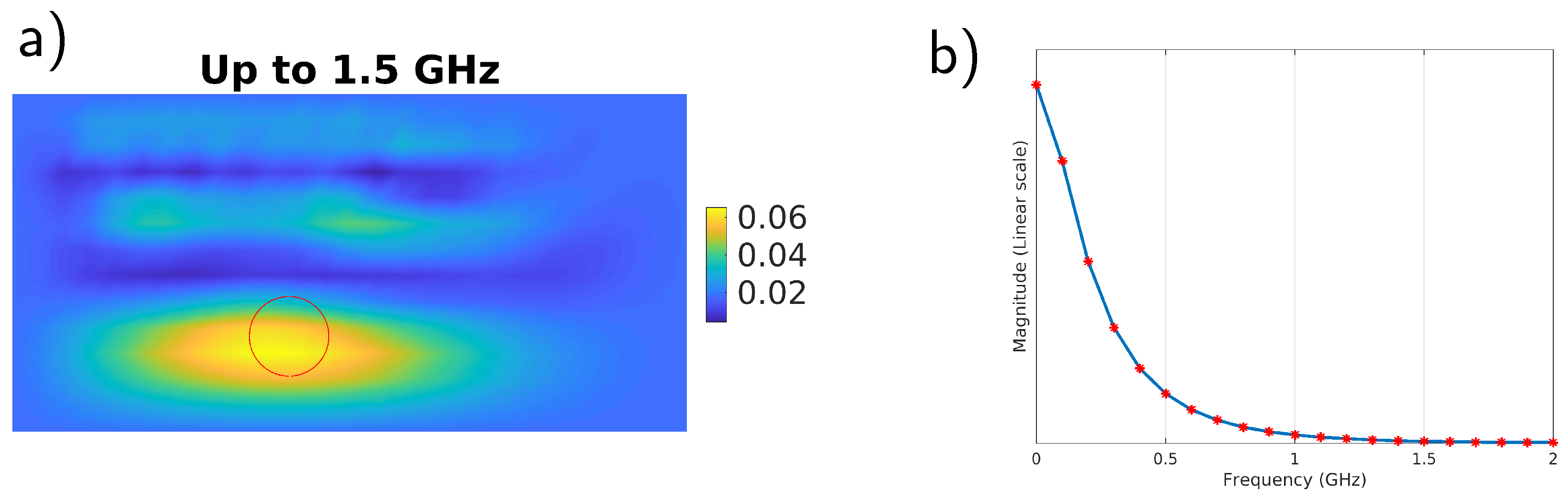
In Figure 18a, the reconstruction obtained by using Fourier transform coefficients from $0\mathrm{MHz}$ up to $1.5\mathrm{GHz}$ in steps of $100\mathrm{MHz}$ is shown. The magnitude of the signal Fourier coefficients are shown at Figure 18b. The results show that using frequencies up to $1.5\mathrm{GHz}$ yields a similar reconstruction to proposed windows. However, if only frequencies lower than $1.5\mathrm{GHz}$ are used the reconstructions suffers from instabilities. This agrees with the results of [45] that suggest that useful information can be found at GHz order.

The relative equivalence of frequency and windows based results can be understood by realizing that in both cases, the complex numbers associated to each frequency are fitted. In the case of Fourier transform datatype, this is done directly, but for temporal windows, this is done by windowing the frequency domain. Nevertheless, there are some important differences. First, as was shown in Section 2.4, by applying the Fourier transform to a noisy signal the noise becomes correlated. This does not occur when not overlapping time windows such as Tukey windows are used. Second, when reconstruction is done directly in frequency domain, the linear system to solve is complex while in the temporal windows case it is real. Third, temporal window-based reconstruction is more intuitive to understand, since it is associated to photon arrival times. Therefore, in many cases, a weight matrix could be built in order to weight some windows over other ones, depending on how noisy they are. This fact makes the problem much more easy to stabilize compared to frequency based reconstructions. Last, in the same fashion as the paper published by Hasnain et al. [36], a system that directly measures a gated DTOF (e.g., using rectangular gates) instead of the full curve could be faster than nowadays time-resolved systems. Moreover, those gated DTOFs could be used in the proposed reconstruction process since they are equivalent to Tukey windows. Such a system could be potentially faster than state-of-the-art time-resolved systems without compromising reconstruction quality.

4. Conclusions

In this paper, a new method has been proposed for computing temporal windows. The technique consists of computing the temporal windows in the frequency domain instead of in time domain. The main advantage is that better temporal selectivity windows can be used, without compromising considerably computational efficiency. To illustrate the method, Tukey and Gaussian windows were used. The obtained results in a numerical phantom prove that these new class of windows have better photon time-arrival selectivity and do not correlate with the noise. As a result, the newly developed method improves the localization and absorption quantification of inclusions at the deep layers of a reflectance geometry. These results have been demonstrated to be equivalent, under certain conditions, to frequency-based reconstruction, when frequencies up to GHz order are used.

References

- Weigl, W.; Milej, D.; Janusek, D.; Wojtkiewicz, S.; Sawosz, P.; Kacprzak, M.; Gerega, A.; Maniewski, R.; Liebert, A. Application of optical methods in the monitoring of traumatic brain injury: A review. J. Cereb. Blood Flow Metab. 2016, 36, 1825–1843. [Google Scholar] [CrossRef] [PubMed]
- Cooper, R.J.; Magee, E.; Everdell, N.; Magazov, S.; Varela, M.; Airantzis, D.; Gibson, A.P.; Hebden, J.C. MONSTIR II: A 32-channel, multispectral, time-resolved optical tomography system for neonatal brain imaging. Rev. Sci. Instrum. 2014, 85, 053105. [Google Scholar] [CrossRef] [PubMed]
- Taroni, P.; Pifferi, A.; Quarto, G.; Spinelli, L.; Torricelli, A.; Abbate, F.; Villa, A.M.; Balestreri, N.; Menna, S.; Cassano, E.; et al. Noninvasive assessment of breast cancer risk using time-resolved diffuse optical spectroscopy. J. Biomed. Opt. 2010, 15, 060501. [Google Scholar] [CrossRef] [PubMed]
- Lindner, C.; Mora, M.; Farzam, P.; Squarcia, M.; Johansson, J.; Weigel, U.M.; Halperin, I.; Hanzu, F.A.; Durduran, T. Diffuse optical characterization of the healthy human thyroid tissue and two pathological case studies. PLoS ONE 2016, 11, e0147851. [Google Scholar] [CrossRef]
- Singer, J.R.; Grünbaum, F.A.; Kohn, P.; Zubelli, J.P. Image Reconstruction of the Interior of Bodies That Diffuse Radiation. Science 1990, 248, 990–993. [Google Scholar] [CrossRef]
- Arridge, S.R.; Schweiger, M.; Delpy, D.T. Iterative reconstruction of near-infrared absorption images. In Inverse Problems in Scattering and Imaging; International Society for Optics and Photonics: Bellingham, WA, USA, 1992; Volume 1767. [Google Scholar]
- Wang, L.V.; Wu, H. Biomedical Optics: Principles and Imaging; Wiley Publisher: Hoboken, NJ, USA, 2007; p. 376. [Google Scholar]
- Liemert, A.; Reitzle, D.; Kienle, A. Analytical solutions of the radiative transport equation for turbid and fluorescent layered media. Sci. Rep. 2017, 7, 3819. [Google Scholar] [CrossRef]
- Liemert, A.; Kienle, A. Analytical solution of the radiative transfer equation for infinite-space fluence. Phys. Rev. A 2011, 83, 015804. [Google Scholar] [CrossRef] [Green Version]
- Liemert, A.; Kienle, A. Exact and efficient solution of the radiative transport equation for the semi-infinite medium. Sci. Rep. 2013, 3, 2018. [Google Scholar] [CrossRef]
- Wang, L.; Jacques, S.L.; Zheng, L. MCML-Monte Carlo modeling of light transport in multi-layered tissues. Comput. Methods Programs Biomed. 1995, 47, 131–146. [Google Scholar] [CrossRef]
- Fang, Q. Mesh-based Monte Carlo method using fast ray-tracing in Plücker coordinates. Biomed. Opt. Express 2010, 1, 165–175. [Google Scholar] [CrossRef]
- González-Rodríguez, P.; Kim, A.D. Diffuse optical tomography using the one-way radiative transfer equation. Biomed. Opt. Express 2015, 6, 2006–2021. [Google Scholar] [CrossRef] [PubMed] [Green Version]
- Tarvainen, T.; Vauhkonen, M.; Kolehmainen, V.; Kaipio, J.P. Hybrid radiative-transfer–diffusion model for optical tomography. Appl. Opt. 2005, 44, 876–886. [Google Scholar] [CrossRef] [PubMed]
- Pierrat, R.; Greffet, J.J.; Carminati, R. Photon diffusion coefficient in scattering and absorbing media. JOSA A 2006, 23, 1106–1110. [Google Scholar] [CrossRef]
- Yamada, Y.; Suzuki, H.; Yamashita, Y. Time-domain near-infrared spectroscopy and imaging: A review. Appl. Sci. 2019, 9, 1127. [Google Scholar] [CrossRef] [Green Version]
- Chu, M.; Dehghani, H. Image reconstruction in diffuse optical tomography based on simplified spherical harmonics approximation. Opt. Express 2009, 17, 24208–24223. [Google Scholar] [CrossRef] [PubMed]
- Ma, W.; Zhang, W.; Yi, X.; Li, J.; Wu, L.; Wang, X.; Zhang, L.; Zhou, Z.; Zhao, H.; Gao, F. Time-domain fluorescence-guided diffuse optical tomography based on the third-order simplified harmonics approximation. Appl. Opt. 2012, 51, 8656–8668. [Google Scholar] [CrossRef] [PubMed]
- Xu, Y.; Gu, X.; Fajardo, L.L.; Jiang, H. In vivo breast imaging with diffuse optical tomography based on higher-order diffusion equations. Appl. Opt. 2003, 42, 3163–3169. [Google Scholar] [CrossRef]
- Arridge, S.R.; Schweiger, M.; Hiraoka, M.; Delpy, D.T. A finite element approach for modeling photon transport in tissue. Med. Phys. 1993, 20, 299–309. [Google Scholar] [CrossRef]
- Hervé, L.; Puszka, A.; Planat-Chrétien, A.; Dinten, J.M. Time-domain diffuse optical tomography processing by using the Mellin-Laplace transform. Appl. Opt. 2012, 51, 5978–5988. [Google Scholar] [CrossRef]
- Arridge, S.R.; Schweiger, M. Direct calculation of the moments of the distribution of photon time of flight in tissue with a finite-element method. Appl. Opt. 1995, 34, 2683–2687. [Google Scholar] [CrossRef] [Green Version]
- Arridge, S.R. Optical tomography in medical imaging. Inverse Probl. 1999, 15, R41. [Google Scholar] [CrossRef] [Green Version]
- Soloviev, V.Y.; McGinty, J.; Tahir, K.B.; Neil, M.A.; Sardini, A.; Hajnal, J.V.; Arridge, S.R.; French, P.M.W. Fluorescence lifetime tomography of live cells expressing enhanced green fluorescent protein embedded in a scattering medium exhibiting background autofluorescence. Opt. Lett. 2007, 32, 2034–2036. [Google Scholar] [CrossRef] [PubMed]
- Dehghani, H.; Srinivasan, S.; Pogue, B.W.; Gibson, A. Numerical modelling and image reconstruction in diffuse optical tomography. Philos. Trans. R. Soc. A 2009, 367, 3073–3093. [Google Scholar] [CrossRef] [PubMed] [Green Version]
- Pogue, B.W.; Patterson, M.S.; Jiang, H.; Paulsen, K.D. Initial assessment of a simple system for frequency domain diffuse optical tomography. Phys. Med. Biol. 1995, 40, 1709. [Google Scholar] [CrossRef] [PubMed]
- Gulsen, G.; Xiong, B.; Birgul, O.; Nalcioglu, O. Design and implementation of a multifrequency near-infrared diffuse optical tomography system. J. Biomed. Opt. 2006, 11, 014020. [Google Scholar] [CrossRef] [Green Version]
- Soloviev, V.Y. Mesh adaptation technique for Fourier-domain fluorescence lifetime imaging. Med. Phys. 2006, 33, 4176–4183. [Google Scholar] [CrossRef]
- Milstein, A.B.; Stott, J.J.; Oh, S.; Boas, D.A.; Millane, R.P.; Bouman, C.A.; Webb, K.J. Fluorescence optical diffusion tomography using multiple-frequency data. J. Opt. Soc. Am. A 2004, 21, 1035–1049. [Google Scholar] [CrossRef]
- Arridge, S.R.; Schweiger, M. Photon-measurement density functions. Part 2: Finite-element-method calculations. Appl. Opt. 1995, 34, 8026–8037. [Google Scholar] [CrossRef] [Green Version]
- Pinsky, M.A. Introduction to Fourier Analysis and Wavelets; American Mathematical Society: Providence, RI, USA, 2002; Volume 102. [Google Scholar]
- Doulgerakis-Kontoudis, M.; Eggebrecht, A.T.; Wojtkiewicz, S.; Culver, J.P.; Dehghani, H. Toward real-time diffuse optical tomography: Accelerating light propagation modeling employing parallel computing on GPU and CPU. J. Biomed. Opt. 2017, 22, 125001. [Google Scholar] [CrossRef] [Green Version]
- Schweiger, M. GPU-accelerated Finite Element Method for Modelling Light Transport in Diffuse Optical Tomography. J. Biomed. Imaging 2011, 2011, 10. [Google Scholar] [CrossRef]
- Liebert, A.; Wabnitz, H.; Grosenick, D.; Möller, M.; Macdonald, R.; Rinneberg, H. Evaluation of optical properties of highly scattering media by moments of distributions of times of flight of photons. Appl. Opt. 2003, 42, 5785–5792. [Google Scholar] [CrossRef] [PubMed]
- Liebert, A.; Wabnitz, H.; Steinbrink, J.; Obrig, H.; Möller, M.; Macdonald, R.; Villringer, A.; Rinneberg, H. Time-resolved multidistance near-infrared spectroscopy of the adult head: Intracerebral and extracerebral absorption changes from moments of distribution of times of flight of photons. Appl. Opt. 2004, 43, 3037–3047. [Google Scholar] [CrossRef] [PubMed]
- Hasnain, A.; Mehta, K.; Zhou, X.; Li, H.; Chen, N. Laplace-domain diffuse optical measurement. Sci. Rep. 2018, 8, 12134. [Google Scholar] [CrossRef] [PubMed]
- Harris, F.J. On the use of windows for harmonic analysis with the discrete Fourier transform. Proc. IEEE 1978, 66, 51–83. [Google Scholar] [CrossRef]
- Wabnitz, H.; Jelzow, A.; Mazurenka, M.; Steinkellner, O.; Macdonald, R.; Milej, D.; Żołek, N.; Kacprzak, M.; Sawosz, P.; Maniewski, R.; et al. Performance assessment of time-domain optical brain imagers, part 2: nEUROPt protocol. J. Biomed. Opt. 2014, 19, 086012. [Google Scholar] [CrossRef]
- Ducros, N.; Hervé, L.; Da Silva, A.; Dinten, J.M.; Peyrin, F. A comprehensive study of the use of temporal moments in time-resolved diffuse optical tomography: Part I. Theoretical material. Phys. Med. Biol. 2009, 54, 7089. [Google Scholar] [CrossRef] [Green Version]
- Ducros, N.; Da Silva, A.; Hervé, L.; Dinten, J.M.; Peyrin, F. A comprehensive study of the use of temporal moments in time-resolved diffuse optical tomography: Part II. Three-dimensional reconstructions. Phys. Med. Biol. 2009, 54, 7107. [Google Scholar] [CrossRef] [Green Version]
- Baltagi, B. Econometrics; Springer: Berlin, Germany, 2008. [Google Scholar]
- Schweiger, M.; Arridge, S.R.; Hiraoka, M.; Delpy, D.T. The finite element method for the propagation of light in scattering media: Boundary and source conditions. Med. Phys. 1995, 22, 1779–1792. [Google Scholar] [CrossRef]
- Zouaoui, J.; Sieno, L.D.; Hervé, L.; Pifferi, A.; Farina, A.; Dalla Mora, A.; Derouard, J.; Dinten, J.M. Chromophore decomposition in multispectral time-resolved diffuse optical tomography. Biomed. Opt. Express 2017, 8, 4772–4787. [Google Scholar] [CrossRef] [Green Version]
- Puszka, A.; Hervé, L.; Planat-Chrétien, A.; Koenig, A.; Derouard, J.; Dinten, J.M. Time-domain reflectance diffuse optical tomography with Mellin-Laplace transform for experimental detection and depth localization of a single absorbing inclusion. Biomed. Opt. Express 2013, 4, 569–583. [Google Scholar] [CrossRef] [Green Version]
- Wojtkiewicz, S.; Durduran, T.; Dehghani, H. Time-resolved near infrared light propagation using frequency domain superposition. Biomed. Opt. Express 2018, 9, 41–54. [Google Scholar] [CrossRef] [PubMed] [Green Version]
- Hansen, P.C. Discrete Inverse Problems: Insight and Algorithms; SIAM: Philadelphia, PA, USA, 2010. [Google Scholar]
Figure 1.
Absorption reconstruction algorithm based on linearized Born equation (Equation (2)).
Figure 2.
(Left) Distribution of photon time of flight (DTOF) and temporal window in time domain. (Right) Magnitude of the Fourier transforms of and ; it is feasible to aproximate numerically the integral in frequency domain since spectra decay rapidly.
Figure 3.
(Left) Different n orders of Mellin-Laplace windows for . (Right) Fourier transform of those windows; as the order n of the Mellin-Laplace moment is increased, its spectrum magnitude is narrower and has less dispersion.
Figure 4.
(Left) Fifth order () Mellin-Laplace window with different p values. (Right) Fourier transform of those windows; as the p value is increased, the magnitude of the Mellin-Laplace window spectrum is more spread.
Figure 5.
(Left) Several Gaussian functions with different values. (Right) Spectrum magnitude of previous Gaussian functions. The more spread the Gaussian function, the narrower its Fourier transform magnitude.
Figure 6.
(Left) Several exponential windows with different p values. (Right) Spectrum magnitude of previous functions.
Figure 7.
(Left) Several Tukey functions with different values. (Right) Spectrum magnitude of previous Tukey functions.
Figure 8.
Correlation matrices of standard moments (first 50 orders), Mellin–Laplace (first 50 orders, ), Gaussian ( ns shifts, ), and Tukey windows ( ns shifts, and ns).
Figure 9.
(Left) Instrumental response function of a single photon avalanche diode detector (SPAD) detector (blue line). Normalized simulated signal without IRF or noise (red line). Normalized simulated signal convoluted with the IRF (yellow line). Normalized simulated signal convoluted with IRF and corrupted with Poisson noise (black line). (Right) Tetrahedral mesh used to generate the synthetic data; it had a size of and was discretized using around 32 and 172 thousand nodes and elements respectively.
Figure 10.
(Left) Scheme of the numerical phantom. Simulated signals were convolved with the IRF of a single photon avalanche diode detector SPAD and corrupted by Poisson noise. (Right) Source positions; red crosses. Detector positions; blue dots. Note that for each source only the signal at two detectors were considered; right and down. For example, for source at position only the signal at detectors and was used.
Figure 11.
Reconstruction algorithm flowchart.
Figure 12.
Black curve represents a simulated DTOF. (a) Mellin–Laplace windows (, 35 moments), note that they are highly overlapped. (b) Gaussian windows (). (c) Tukey windows (, ns).
Figure 13.
Absorption, , reconstructions using Mellin–Laplace, Tukey and Gaussian windows for inclusions from to deep. The red circle indicates the correct location of the inclusion.
Figure 14.
Figure 15.
Mellin-Laplace (blue), Tukey (red) and Gaussian (yellow). Quantitative evaluation metric values for each window and inclusion depth. For localization error and relative reconstructed volume, the standard error shadows indicate the uncertainty given by selecting interest regions whose thresholds range from 60% to 80% of maximum absorption.
Figure 16.
(a) Number of iterations until convergence for Mellin–Laplace and Gaussian windows. (b) Seconds per iteration for Mellin–Laplace windows, novel approach (with Gaussian) and full–time resolved approach.
Figure 17.
(a) Reconstructions for Mellin–Laplace and Tukey windows from same simulated data as Figure 13; cross–Born approach was used to deal with instrumental factors such as IRF or photon noise. The red circle indicates the correct location of the inclusion. (b–d) Quantitative metrics for cross-Born based reconstructions.
Figure 18.
(a) Absorption reconstructions for 3.5 cm deep inclusion using up to frequencies. (b) Magnitude of the signal Fourier coefficients.