Toward Bridging Future Irrigation Deficits Utilizing the Shark Algorithm Integrated with a Climate Change Model

Abstract

Climate change is one of the most effectual variables on the dam operations and reservoir water system. This is due to the fact that climate change has a direct effect on the rainfall–runoff process that is influencing the water inflow to the reservoir. This study examines future trends in climate change in terms of temperature and precipitation as an important predictor to minimize the gap between water supply and demand. In this study, temperature and precipitation were predicted for the period between 2046 and 2065, in the context of climate change, based on the A₁B scenario and the HAD-CM3 model. Runoff volume was then predicted with the IHACRES model. A new, nature-inspired optimization algorithm, named the shark algorithm, was examined. Climate change model results were utilized by the shark algorithm to generate an optimal operation rule for dam and reservoir water systems to minimize the gap between water supply and demand for irrigation purposes. The proposed model was applied for the Aydoughmoush Dam in Iran. Results showed that, due to the decrease in water runoff to the reservoir and the increase in irrigation demand, serious irrigation deficits could occur downstream of the Aydoughmoush Dam.

1. Introduction

Water and energy shortage are essential issues for future society. Decision-makers should suggest changes in the amounts of resources needed based on the demand of a given society [1]. Climate change affects the management of water resources in a way, causing flood or draught which is resulting in severe issues to the environment. Thus, it is necessary to consider climate change for water resource management [2,3,4,5]. Kling et al. [6] simulated runoff in the upper Danube basin and used nonlinear programming to manage the environmental demands in a future period (2011–2030). The results indicated that the volumetric reliability index in the forthcoming period decreased significantly because the total precipitation in future periods considerably reduced; therefore, less inflow to the reservoir occurred.

1.1. Background

One of the critical issues in water resource management is reservoir operation, which requires that both downstream demands are met and that reservoir storage is adequate for critical periods [7,8,9,10,11]. The challenges of a reservoir operation could be solved by an optimization framework. Different methods exist for solving reservoir operation issues in water resources management [12,13]. Traditional methods, such as nonlinear programming, linear programming, and dynamic programming, have been used in previous studies [14,15,16].

Recently, new methods, such as evolutionary algorithms and metaheuristic algorithms, have been used for reservoir operation [17]. Reddy [18] used a genetic algorithm for reservoir operation in India. The aim of the study was to meet downstream irrigation demands, and the results showed that the genetic algorithm did effectively satisfy these demands better than dynamic programming methods. Afshar et al. [19] used the honey bee mating optimization method for reservoir operation, and the results showed that the method converged faster than the genetic algorithm. Bozorg-Hadad et al. [20] also used the honey bee mating optimization algorithm for multi-reservoir operations, and the results showed that the average solution of the method was close to the global solution of the problem. Chang and Cheng [21] used the genetic algorithm for a multi-reservoir system with multiple purposes. Results showed that the genetic algorithm yielded a higher reliability index and adequately satisfied different demands. Fallah-Mehdipour et al. [22] used genetic programming and a genetic algorithm to determine a water release policy. Results showed that the genetic programming method met all requirements, with low vulnerability among different demands.

The bat algorithm, one of the more common methods, was also utilized by Bozorg-Hadad et al. [23] for power plant operation. Results showed that the bat algorithm was superior to other metaheuristic algorithms in finding optimal solutions for more power generation. Thus, different studies have shown that various evolutionary algorithms displayed high performance in solving complex problems. However, these studies did not consider the crucial effects of climate change or reservoir operations, and few studies have found the impact of climate change on reservoir operations. Ashofteh et al. [24] optimized the performance of an irrigation system based on genetic programming in the context of climate change. The period of 1987–2000 for Aidoghmoush dam in East Azerbaijan, Iran was considered the base period for their study, and the period 2026–2039 was considered the future period. Results indicated that the runoff volume and reservoir inflow decreased in the forthcoming period and that future demand also increased. Thus, a notable deficit was observed in the future period. Jahandideh-Tehrani et al. [25] optimized multi-reservoir operations of the Karoon Reservoir System to increase power generation in base and future periods, with the results indicating that the release of water in the future period (2011–2030) decreased because inflow to the reservoir decreased. Additionally, power generation in the future period was less than that of the base period (1971–1990), and the released water was considered a decision variable. Ahmadi et al. [26] extracted the trends from a base period and future period to increase power generation at a power plant of Karoon-4 reservoir in Iran. Results indicated that the vulnerability index of the coming period increased while the reliability index decreased based on a multiobjective genetic algorithm. Moreover, inflow to the reservoir significantly decreased due to lower runoff volume, and subsequently, power generation in the future period experienced considerable issues. Tzabiras et al. [27] used a particle swarm algorithm to provide an optimal solution for decreasing the deficit of an irrigation system in base and future periods on Lake Karla Watershed. Released water was considered a decision variable, and the results indicated that the vulnerability index increased compared to that in the base period due to increased demand in the future period. Yang et al. [28] optimized a multipurpose system based on a genetic algorithm in base and future periods to manage irrigation and environmental demands. Results indicated that the extracted trends in the future period (2011–2030), based on the genetic algorithm, could not meet needs because the drought index increased and precipitation significantly decreased. Ehteram et al. [29] optimized an irrigation system based on a bat algorithm in base and future periods. Results reflected the uncertainty of climate change, and the random parameters in the bat algorithm were important factors that influenced reservoir operation and reservoir storage in the future period (2011–2030). They noted that these factors should be optimized to effectively meet irrigation demand.

Ehteram et al. [30] proposed the shark algorithm to evaluate its performance in solving the real-life, complex problems of optimizing operations of the single reservoir and hypothetical multi-reservoir case studies. The hydrological features and characteristics of the selected case studies were relatively simple and, more specifically, the reservoir’s inflow pattern was almost deterministic, which was considered as one of the major influential parameters in the dam and reservoir operations. Furthermore, a complete lack of an associated series of penalty functions against violations of the operation was assumed in Ehteram et al. [30]. On the other hand, the proposed shark algorithm examined in the current, selected case study, displayed highly nonlinear characteristics in the reservoir system, and a highly stochastic nature in the reservoir’s inflow pattern. Besides, the proposed shark algorithm will be examined, considering three different levels of penalties during the generation of the operation rule. It is regarded as a further challenge for the shark algorithm to adapt these penalty functions and successfully generate optimal operation rules. In this context, this research could be viewed as a further examination of the shark algorithm in creating an optimal operation release policy for dams and reservoirs under different levels of complexity.

1.2. Objective

In this study, climate change and reservoir operation were considered. First, the climate of the Aidoghmoush region of Iran was simulated. Maximum and minimum temperatures and precipitation amounts were simulated based on the Long Ashton Research Station Weather Generator (LARS-WG5) model, which can effectively simulate climate change. Notably, Khajeh et al. [31] investigated the effect of climate change for the period 2011–2040 using this model. Results indicated a reduction in the normal water level in the reservoir. Additionally, LARS-WG5 was used to simulate precipitation for the period 2040–2070 [32]. In the current study, LARS-WG5 was used for climate change predictions, and the volume of runoff was calculated using IHACRES software based on simulated temperature and precipitation. Runoff volume was considered as the inflow to the reservoir, and reservoir operation was simulated with the objective of minimizing the irrigation deficit. The shark metaheuristic algorithm is proposed for reservoir operation, and the decision variable was the water release rate. There was a need to identify the reservoir’s future inflow pattern in order to generate the operation rule for the dam and reservoir water system. In fact, the available parameter for downscaling of the LARS-WG was ‘rainfall’, which could be used to estimate or predict reservoir inflow. Hence, the procedure carried out in this study downscaled precipitation, so that reservoir inflow could be generated using the rainfall-runoff model ‘IHACRES’.

2. Methods

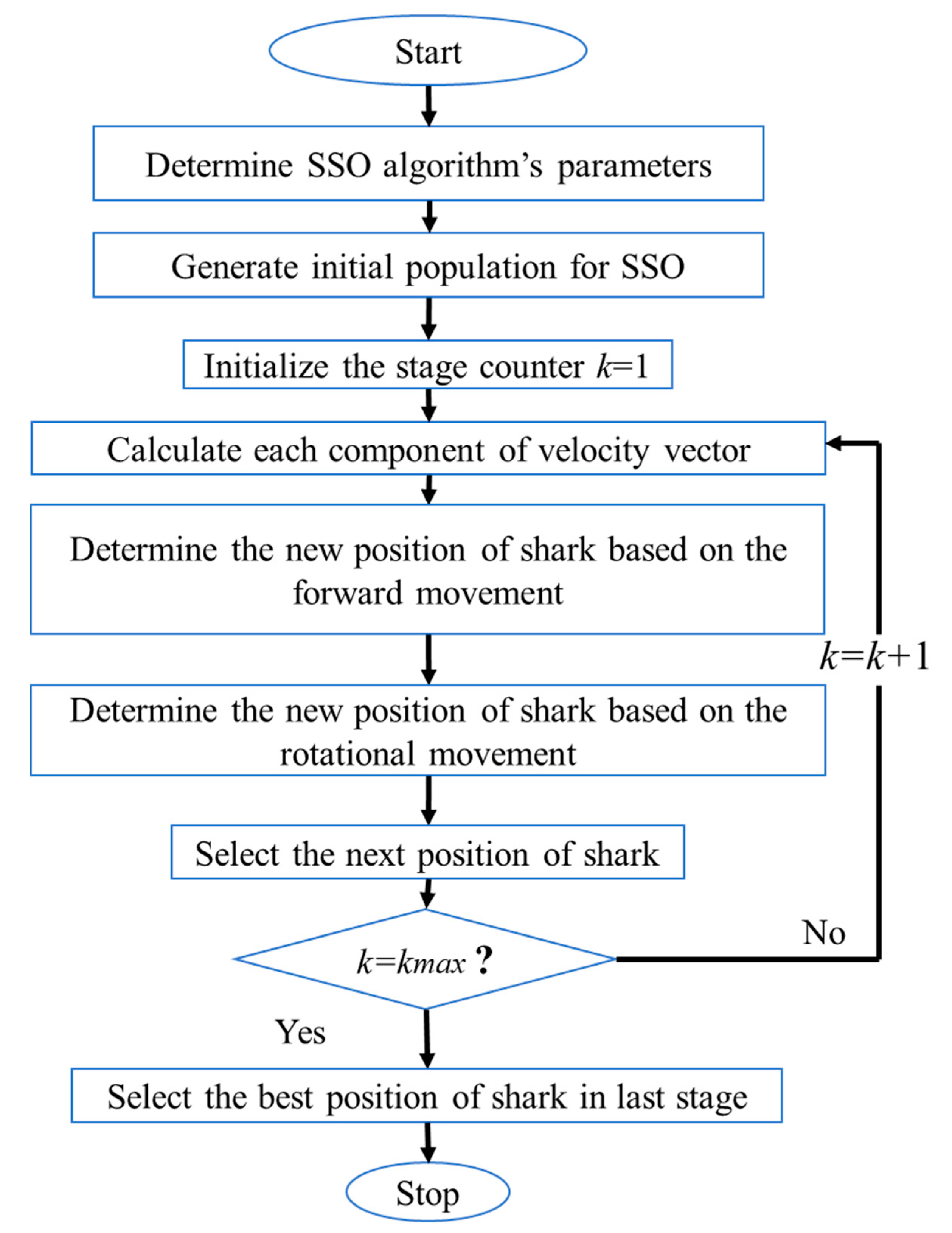
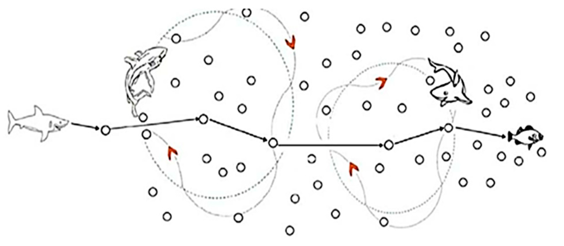
2.1. Shark Algorithm

The shark algorithm is based on olfactory sensors, which can identify the location of prey based on received concentrations of odors. If a fish has been injured and bleeds in the water, the olfactory sensors in sharks can find the position of the fish, as prey, based on the received odor. Thus, the following assumptions are considered in the shark algorithm [33]:

1-

Fish, as the prey of sharks, have been injured, and their bodies distribute blood. Thus, the wounded fish have a low velocity in the water.

2-

Blood is regularly distributed in the water, and the odor particles that are closer to the fish allow the sharks to find the injured fish sooner.

3-

There is a blood resource for each shark that each shark should find.

Figure 1 shows the flowchart of the shark algorithm. First, an initial population of SSO (simplified swam optimization) is considered, and their positions are given as $\left[X_1^l,X_2^l,\dots ,X_{NP}^l\right]$, Where each X is considered a solution candidate. Additionally, each solution candidate has some decision variables, such as $X_i^l=\left[x_{i1}^1,x_{i2}^1,\dots ,x_{iND}^1\right]$, Where x¹_i,j is associated with the j^th decision variable. Then, the velocity of each shark is defined based on $\left[V_1^1,V_2^1,\dots ,V_{NP}^1\right]$, and each velocity encompasses some decision variables, such as $V_1^i=\left[v_{i,1}^1,v_{i,2}^1,\dots ,v_{i,ND}^1\right]$. The shark finds prey based on the intensity of the received odors. Thus, if a shark gets a high-intensity odor, it moves at a higher velocity. Thus, the velocity can be defined based on the changes in the objective function and the intensity of the received odor [33].

$$V_i^k={\eta }_k·R_1·\nabla \left(OF\right){|}_{X_i^k}$$

(1)

where OF is the objective function, ${\eta }_k$ is a coefficient in the range of [0, 1], R₁ is a random value, and k is the number of movements a shark makes toward prey.

The velocity of a shark can be formulated based on the equation

$$v_{i,j}^k={\eta }_k·R_1·\frac{\partial \left(OF\right)}{\partial x_j}|x_{i,j}^k$$

(2)

The inertia of a shark has a limit, and thus, the limit inertia is used for the velocity in Equation (3)

$$v_{i,j}^k={\eta }_k{R}_1\frac{\partial F}{\partial x}{|}_{x_{i,j}^k}+{\alpha }_k·R_2·v_{i,j}^{k-1}$$

(3)

where ${\alpha }_k$ is the limit inertia and R₂ is a random coefficient in the range of [0, 1]. The added inertial term causes the velocity at the current time to be dependent on that at the previous time. Additionally, the speed of a shark has a limit. Specifically, the maximum velocity of a shark is 80 km/h, and the minimum velocity is 20 km/h. Additionally, a limiting coefficient of velocity is used. This coefficient is based on a ratio of 80/20 and is added to the previous equation as β

$$\left|v_{i,j}^k\right|=\min \left[{\left|{\eta }_k·R_1·\frac{\partial \left(OF\right)}{\partial x_j}\right|}_{x_{i,j}^k}+{\alpha }_k·R_2{v}_{i,j}^{k-1}|,\left|{\beta }_k·v_{i,j}^{k-1}\right|\right]$$

(4)

where ${\beta }_k$ is the limit velocity.

The position of a shark in each level is updated based on the equation

$$Y_i^{k+1}=X_i^k+V_i^k\Delta t_k$$

(5)

where $Y_i^{k+1}$ is the location of a shark at the new level and $X_i^k$ is the position of a shark at the previous level.

Additionally, a rotational movement is considered a local search in the shark algorithm (Figure 2). A rotational movement in the shark algorithm is a closed contour that should not be circular but can be a curve. Based on rotational movement, the shark searches the probable best location as a contour so that it can avoid local optimums based on more searches. This process provides accurate searches that allow the shark to obtain a global solution

$$Z_i^{k+1,m}=Y_i^{k+1}+R_3{Y}_i^{k+1},m=1,\dots ,M$$

(6)

where $Z_i^{k+1,m}$ is the position of the shark after a local search, m is the number of points included in a local search, M is the number of points that a shark considers in a local search, and R₃ is a random value between −1 and 1. If a maximization problem is considered, Equation (7) reflects the best solution for all sharks.

$$X_i^{k+1}=\arg \left(\max \right)\{OF\left(Y_i^{k+1}\right),OF\left(Z_i^{k+1}\right),\dots , OF\left(Z_i^{k+1,m}\right)\}$$

(7)

2.2. LARS-WG Model

Different methods are used for the generation of climate change scenarios. In this study, general circulation models were used to simulate climate change. These models are three-dimensional and based on physical and mathematical relations. First, tributary models were simulated; then, all the tributary models of oceans and atmosphere were combined. One of the weaknesses of these models is related to the large scale of computational cells in the temporal and spatial domains. Thus, the associated variables did not have sufficient accuracy for simulating climate change. Different methods, such as the LARS-WG model, were used to downscale computational cells. Additionally, emission scenario A₁B and the HAD-CM3 model were selected to simulate climate change. The A₁B scenario considered rapid future economic and population growth. Specifically, maximum population growth occurs in the current half-century, and the population increase will then decelerate. Additionally, technological advancements will rapidly occur in the future period. A previous study of climate change in the Aidoghmoush basin showed that the A₁B scenario and HAD-CM3 model exhibited good performance compared to other models and scenarios. Ashofteh et al. [34] investigated the uncertainty of different climate models and computed the weights of the different climate change models and scenario models presented. They found that the HAD-CM3 model and A₁B scenario had the highest weights and lowest uncertainty for computations of temperature and precipitation. Additionally, other previous studies in the basin found that the HAD-CM3 model and A₁B scenario yielded the best results among various models and scenarios [24,34].

Two significant steps should be carried out to set up the LARS-WG model considering future periods with downscaling of the GCM data. The first step is to create a data file that defines the estimated behavior of the historical climatic parameters during particular previous periods (*.wg). The second step is to adapt to the selected climate change scenario (*.sta). To complete this step, the three different climate parameters—precipitation, temperature, and radiation—should be computed utilizing Atmosphere-Ocean General Circulation Model (AOGCM) and considering the following features:

-

Once all of the above parameter data files have been completed using (*.sce), all the required data are ready to use the LARS-WG model;

-

The average monthly rate of changes of wet and dry events;

-

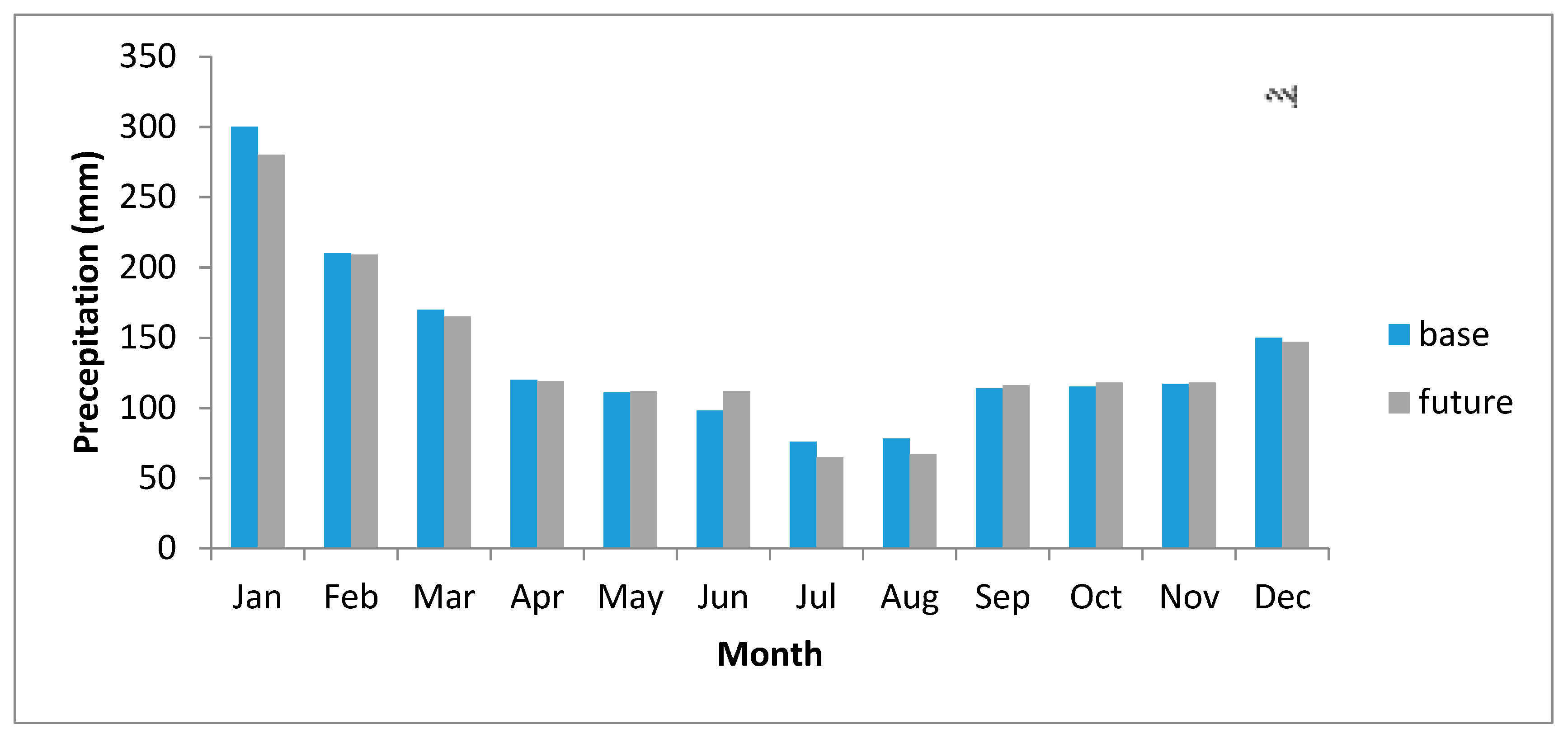
Rate of change of the average monthly precipitation considering the long-term period;

-

Rate of change of the daily temperature (fluctuations) considering the long-term period;

-

The absolute difference of maximum and minimum monthly average temperature;

-

Absolute change of the monthly average radiation (long-term).

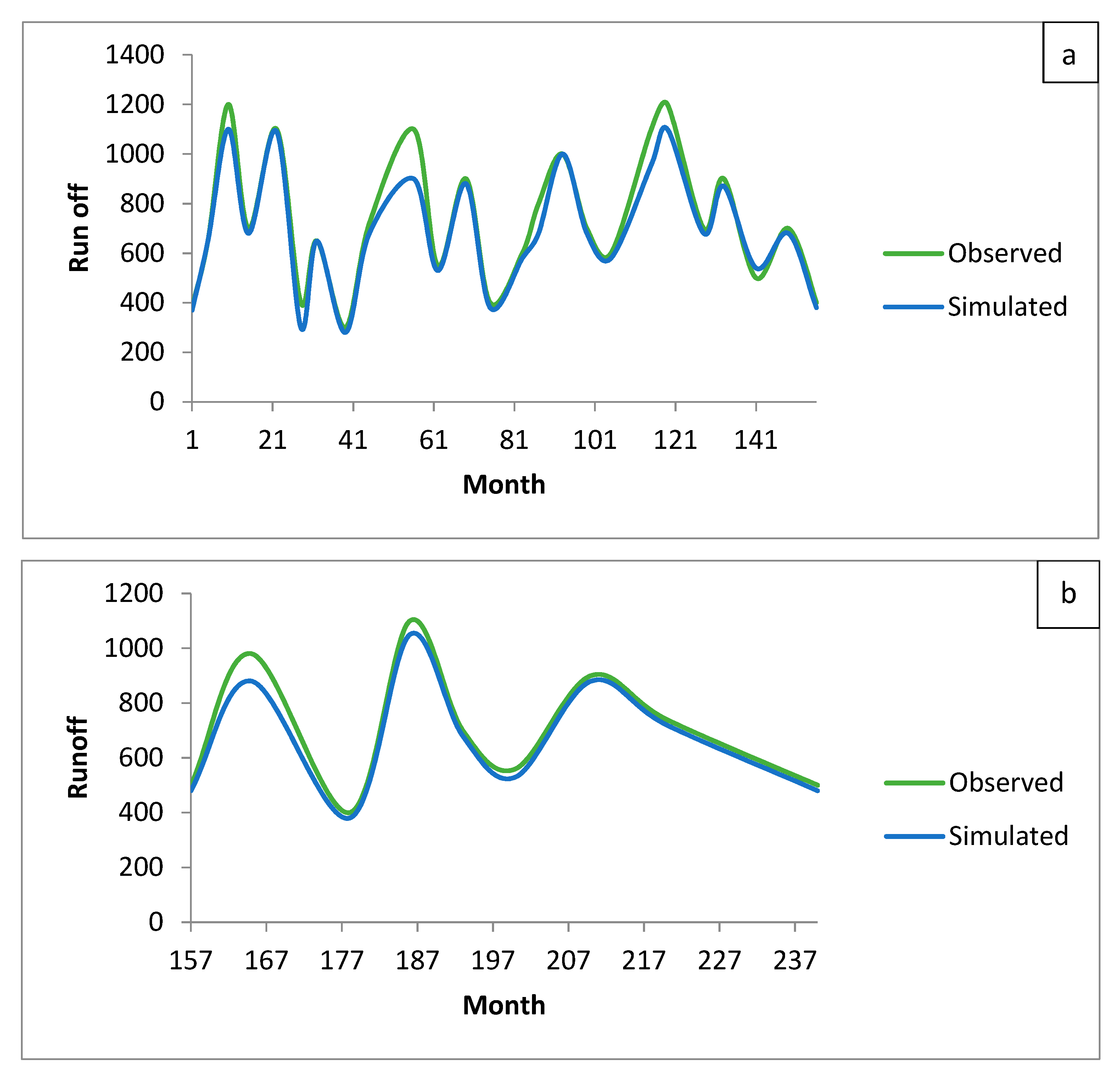
The LARS-WG model can be used to produce daily values of maximum and minimum temperature, precipitation, and radiation, or the number of sunny hours. The first version of this model was used to evaluate agricultural risk [35]. The Markov chain is used for modelling precipitation in the LARS-WG model. LARS-WG uses complex statistical distributions to predict meteorological variables. Specifically, the LARS-WG model receives climate data from the climate model (HAD-CM3); then, the specific scenario for each network in the HAD-CM3 model is considered. A model run requires information from the previous, or base period. This climate change information for the basin and the input from the HAD-CM3 model are subsequently used to simulate climate change conditions for future periods. Thus, the LARS-WG model is considered a black box model [36,37,38].

Main variables in these models are the numbers of wet and dry days and daily precipitation; associated distances are divided equally in the empirical distributions. Radiation in this model is simulated independently from temperature. The amount of precipitation in the current month is based on the semi-empirical distribution in the current month, which is independent of the wetness series, or the amount of precipitation from the previous day. A Fourier series is used for temperature prediction. Maximum and minimum temperatures are simulated based on a random process with average and daily deviations that are dependent on the given conditions, such as dry or wet conditions.

Generation of data is based on three steps. (1) First, the data from a general circulation model, such as HAD-CM3, are extracted; then, a scenario for each network in the HAD-CM3 model is defined. (2) Performance of LARS-WG is evaluated based on the condition of climate change in a base period or past periods. (3) The model is used to predict climate change conditions for future periods. Additionally, the following indices are used to assess model accuracy in the prediction of maximum and minimum temperatures and precipitation:

$$R^2=\frac{{\left[{{\displaystyle \sum }}_{i=1}^n\left(X_i-\stackrel{-}{X}\right)\left(Y_i-\stackrel{-}{Y}\right)\right]}^2}{{{\displaystyle \sum }}_{i=1}^n\left(X_i-\stackrel{-}{X}\right){{\displaystyle \sum }}_{i=1}^n{\left(Y_i-\stackrel{-}{Y}\right)}^2}$$

(8)

$$RMSE=\sqrt{\frac{{{\displaystyle \sum }}_{i=1}^n{\left(X_i-Y_i\right)}^2}{n}}$$

(9)

$$MBE=\frac{{{\displaystyle \sum }}_{i=1}^n\left(X_i-Y_i\right)}{n}$$

(10)

where R² is the coefficient of determination, RMSE is the root mean square error, MBE is the mean absolute error, X is the simulated value, Y is the observed value, $\overline{X}$ and $\overline{Y}$. The mean value for simulated and observed and n is the number of values.

2.3. IHACRES Model

The IHACRES runoff-precipitation model is a conceptual and lumped model. Previous studies have shown that the IHACRES model requires fewer inputs and is mathematically more straightforward than other hydrological models [24,34]. Additionally, an investigation of the uncertainty associated with runoff simulation based on different hydrological models showed that the uncertainty of the IHACRES model is comparable to that of other hydrological models [24,29,39].

This model is based on a nonlinear loss module and a linear unit hydrograph. First, the temperature (t_k) and precipitation (r_k), which are based on the nonlinear loss module, are converted to effective rainfall. Subsequently, rainfall is converted to surface runoff based on the linear unit hydrograph module. The equation used in the nonlinear module is based on the following equations:

$$u_k=s_k\times r_k$$

(11)

$$s_k=C\times r_k+\left[1+\frac{1}{{\tau }_w\left(t_k\right)}\right]s_{k-1}$$

(12)

$${\tau }_w\left(t_k\right)={\tau }_w{e}^{0.062\left(R-t_k\right)}$$

(13)

$$x_k=a^q{x}_{k-1}+b^q{u}_{k-1}+a^s{x}_{k-1}+b^s{u}_{k-1}$$

(14)

where s_k is the wet index for the basin, ${\tau }_w\left(t_k\right)$ is the control parameter of the s_k value when precipitation does not occur, R is the reference temperature, C is a parameter related to runoff and effective rainfall, and x_k is a runoff.

The parameters ${\tau }_w$, C, a, and b are computed based on the calibrated and observed data.

3. Case Study

The Aidoughmoush Dam is located in the city of Mianeh, Azerbaijan Province, Iran. As shown in Figure 3, the dam was constructed on the Aidoughmoush River in the Caspian catchment. The primary purpose of the dam is to supply irrigation water for the region, of which 15 × 10³ ha is cultivated land. The maximum and minimum storage volumes for this dam are 145.7 × 10⁶ m³ and 8.9 × 10⁶ m³, respectively.

The objective function involves minimizing the irrigation deficit

$$Minimize\left(OF\right)={\displaystyle \sum }_{t=1}^{T{\sum }^2}\left(\frac{D_t-R_t}{D_{max}}\right)$$

(15)

where D is the demand, R is the quantity of released water, and D_max is the maximum demand.

The continuity equation for this reservoir is based on the equation

$$S_{t+1}=S_t+I_t-los{s}_t-R_t-S{p}_t$$

(16)

where S_t+1 is the storage at time t + 1; I_t is the inflow to the reservoir; loss_t represents the total losses, such as evaporation, and Sp_t is the dam overflow.

The loss is computed based on the equation

$$Los{s}_t=A_t\times E{V}_t$$

(17)

where A_t is the area of the reservoir and EV is the value of evaporation.

Additionally, the value of dam overflow is computed based on the equation

$$S{p}_t=\left[\begin{array}{l}0\leftarrow if\left(S_t\right)\le S_{max}\\ St{\left(S_t\right)}_{{max}_{max}}\end{array}\right]$$

(18)

In addition, the following constraints should be considered for the stored and released quantities of water.

$$0\le R_t\le D_{t}S{t}_{{max}_{min}}$$

(19)

Furthermore, if the constraints are not satisfied, penalty functions should be added to the objective function as follows:

$$P_{1,t}=\left[\begin{array}{l}0\leftarrow if\left(S_{t+1}>S_{\min }\right)\\ \frac{{\left(S_{\min }-S_{t+1}\right)}^2}{S_{\max }}\leftarrow otherwise\end{array}\right]$$

(20)

$$P_{2,t}=\left[\begin{array}{l}0\leftarrow if\left(S_{t+1}\right)<S_{\max }\\ \frac{{\left(S_{t+1}-S_{\max }\right)}^2}{S_{\max }}\leftarrow otherwise\end{array}\right]$$

(21)

$$P_{3,t}=\left[\begin{array}{l}0\leftarrow if\left(R_t\right)<D_t\\ \frac{{\left(R_t-D_t\right)}^2}{D_{\max }}\leftarrow otherwise\end{array}\right]$$

(22)

The following steps are used for reservoir optimization:

Step 1: First, scenario A₁B and the HAD-CM3 model are used to simulate climate change based on the LARS-WG5 model.

Step 2: The model is evaluated based on the predicted maximum and minimum temperatures and precipitation for the base period (1980–1999).

Step 3: Then, the climate change model is used to calculate the temperatures and precipitation in the future period.

Step 4: Next, the IHACRES model uses the computed temperatures and precipitation from Steps 2 and 3 to estimate runoff.

Step 5: The computed runoff from the previous step is used as inflow into the reservoir, and reservoir operation based on the shark algorithm begins.

Step 5: Additionally, the following indices are considered to evaluate the water supply for the base and future periods based on the shark algorithm.

• Reliability index

The reliability index reflects the ratio of water demand to the quantity of released water for one operation period [29,39].

$${\alpha }_V=\frac{{\displaystyle \sum _{t=1}^T{R}_t}}{{\displaystyle \sum _{t=1}^T{D}_t}}\times 100$$

(23)

• Vulnerability index

The vulnerability index reflects the maximum probability of failure in an operation period [29,39]:

$$\lambda =Ma{x}_{t=1}^T\left(\frac{D_t-R_t}{D_t}\right)$$

(24)

where $\lambda$ is the vulnerability index.

• Resiliency index

The resiliency index reflects the ability of a system to avoid failure [29]:

$${\gamma }_i=\frac{f_{si}}{F_i}$$

(25)

where ${\gamma }_i$ is the resiliency index, $f_{si}$ is the number of failure series in the operation period, and $F_i$ is the number of the failure periods.

4. Results and Discussion

Figure 4 shows a comparison of the simulated maximum and minimum temperatures versus the observed data. Temperatures are average values for the period 2046 to 2065. Notably, the observed and simulated data coincide, and

Table 1. Statistical analysis for predicted temperature in the base period.

Parameter	R2	RMSE	MBE
Maximum temperature	0.94	4	2
Minimum temperature	0.96	3.5	1.5

shows a statistical analysis of the simulated temperatures. Different indices in Table 1 reflect the high accuracy of the climate change model in simulating temperatures. Figure 5 shows the simulated temperatures for the future period (2046–2065). Temperatures for the coming period were compared to those for the base period (1980–1999). The average minimum temperature in the winter season increased by 33% compared to that in the base period. Additionally, the average minimum temperature in the spring season increased by 20% compared to that in the same season in the base period. Moreover, the average minimum temperatures in summer and autumn increased by 4% and 9.64%, respectively. Thus, the minimum temperature increased overall. The average maximum temperature increased by 14% for the winter season and by 17% for the spring season. Additionally, the average maximum temperatures in the summer and autumn seasons increased by 5% and 1.6%, respectively. Thus, the maximum temperature increased overall for the future period. Figure 6 shows the simulated values of precipitation. Results highlighted the accuracy of the proposed climate change model because the observed and simulated data coincided. Also, the R², RMSE and MBE values of the climate change model were 0.97, 4, and 3 mm, respectively, for the precipitation prediction. These results reflected the high accuracy of the applied model. Figure 7 shows simulated precipitation for the future period. Average precipitation totals in the winter and spring seasons decreased by 3.6% and 0.75%, respectively, compared to those for the base period. Moreover, the average precipitation totals in summer and autumn decreased by 3.7% and 1.6%, respectively. Thus, the precipitation totals decreased overall for the future period.

The total period of the data set that has been used to examine the IHACRES model was 20 years monthly (12 × 20 = 240 records). The IHACRES model has a few parameters that needed to be tuned to achieve accurate prediction for the runoff value (reservoir’s inflow). In order to identify the correct values for these IHACRES model’s parameters, there was a need to calibrate and validate the model. Therefore, the collected data set was split into different data sets; 156 records were used to calibrate the model and achieve the correct value of the IHACRES model’s parameters. Then, using the calibrated IHACRES model to predict runoff using the unseen 84 records to validate the achieved accuracy. The primary purpose of this step was to assure that when the model will be used for future records (downscaling records in future period), the accuracy of the runoff (reservoir’s inflow) would be near to the real value.

Figure 8 illustrates the performance of the IHACRES model in simulating runoff volume. A total of 156 periods were considered in the calibration of this model, and 84 periods were used for verification. Figure 9 shows the predicted runoff volumes for the base and future periods. Runoff volumes in the winter and spring seasons decreased by 4% and 23%, respectively, compared to those in the base period. In addition, runoff volumes in summer and autumn decreased by 4.7% and 3.3%, respectively, compared to those in the base period.

Table 2. Statistical analysis for predicted runoffs in the base period.

Parameter	R2	RMSE (106 m3)	MBE (106 m3)
Calibration	0.96	3	1
Verification	0.92	5	3

shows a statistical analysis of simulated runoff. Since the coefficient of determination for the runoff volume was 0.96 in the calibration stage, IHACRES was shown to be effectively applied for runoff simulation. Additionally, the RMSE and MBE values were negligible.

Table 3. Sensitivity analysis for reservoir optimization.

Base Period
Population Size	Objective Function	α	Objective Function	M	Objective Function
10	1.454	0.58	1.565	10	1.454
30	1.312	0.68	1.476	20	1.412
50	1.455	0.78	1.312	30	1.311
70	1.576	0.88	1.415	40	1.398
Future Period
10	1.678	0.58	1.594	10	1.611
30	1.612	0.68	1.525	20	1.567
50	1.525	0.78	1.567	30	1.525
70	1.567	0.88	1.578	40	1.545

presents a sensitivity analysis of the shark algorithm in the base and future periods. The optimal population size for the shark algorithm, which is based on minimization the objective function in the base period, is 30, and M is also 30 in this period. M is the number of points investigated in a local search by sharks. Additionally, the value of $\alpha$ is 0.78 for the base period. In the future period, the optimal population size for the shark algorithm is 50, the best value M value is 30, and the value of $\alpha$ is 0.68.

Table 4. 10 random results of the shark algorithm for the future and base periods.

Run	Base Period	Future Period
1	1.455	1.529
2	1.457	1.525
3	1.455	1.525
4	1.455	1.525
5	1.455	1.525
6	1.455	1.525
7	1.455	1.525
8	1.455	1.525
9	1.455	1.525
10	1.455	1.525
Average solution	1.455	1.525
Variation coefficient	0.0006	0.0008
Global solution	1.454

shows the results for 10 random runs of the shark algorithm for the base and future periods. The average solution for the base period was less than that for the future period. Moreover, the global solution of the problem was obtained using Lingo software (Lingo, 2010) and a nonlinear programming method. Results indicated that the average solution of the shark algorithm for the base and future periods was 0.99% of the global solution. Furthermore, the coefficients of variation were small for both periods. This finding suggests that the shark algorithm provides high-quality solutions. Evapotranspiration associated with each crop should be calculated to compute the irrigation demand. Therefore, evapotranspiration was computed based on the crop coefficient and reference crop evapotranspiration. However, the necessary data were not available for the future period; thus, the reference crop evapotranspiration was computed based on another method. First, a regression relationship between the temperature and reference crop evapotranspiration was obtained for the base period. Then, this equation was used to compute the reference crop evapotranspiration for the future period based on the simulated temperatures for the future period. Next, the following equation was used to calculate crop evapotranspiration by

$$E{T}_C=K_{C_t}\times E{T}_0$$

(26)

where $E{T}_C$ is evapotranspiration, $K_{C_t}$ is the crop coefficient, and $E{T}_0$ is the reference crop evapotranspiration.

Subsequently, effective rainfall was computed based on the equation

$$\begin{array}{l}{P}_e=\frac{P_t}{125\times \left(125-0.2P_t\right)}\leftarrow P_t\le 250 \mathrm{mm}\\ P_e=125+0.1\times P_t\leftarrow P_t\ge 250 \mathrm{mm}\end{array}$$

(27)

where P_e is effective rainfall and P_t is rainfall.

Equation (27) is taken from the Soil Conservation Service. Next, the net volume of water was computed based on the equation

$$W{R}_t=E{T}_C-P_e$$

(28)

Then, the volume of the demand was calculated based on the equation

$$V_t=\frac{W{R}_t\times 10\times A}{1000000}$$

(29)

where V_t is the volume of the demand and A is the cultivated area.

Water demand for the future was computed based on Equation (29). In this equation, the effective rainfall is computed based on Equation (27) and generated rainfall by climate change models and scenarios. Evapotranspiration, based on Equation (26), was then computed. The reference crop evapotranspiration was based on Penman–Monteith, and the crop coefficient was calculated based on mean relative humidity, wind speed, and information about the growth periods of crops.

Figure 10 shows the demand volume for irrigation based on computed climate variables. Demands increased by approximately 27% in the future period. Figure 11 shows the quantity of released water in the base and future periods, and this quantity was 8.34% less in the future period than in the base period. However, irrigation demand in the future period was higher than that in the base period; thus, the corresponding deficits were larger. Figure 12 presents the storage values for the base and future periods. Specifically, storage in the future period was 1.21% less than that in the base period because more water was released in the future period than in the base period. Figure 13 shows the convergence for the base and future periods; the objective function for the base period converged faster.

Table 5. Different indices for reservoir operation.

Index	Reliability	Vulnerability	Resiliency
Base	96%	14%	34%
Future	89%	22%	27%

shows the demand-supply for the base and future periods. Reliability index values for the base period were greater than those for the future period because irrigation demand increased over time. Additionally, more water was released in the base period than in the future period. Thus, demands were better met in the base period. Moreover, vulnerability/resiliency index values in the base period were less/more than those in the future period.

A new climate change scenario was investigated to present the ability of the proposed procedure to generate different solutions for the optimal operation rule and strategies for the dam and reservoir water system. The fifth assessment report of the intergovernmental panel (IPCC) was about new scenarios based on specific radiative forcing. These scenarios are known as representative concentration pathways (RCP). One of these scenarios is known as RCP 8.5, which is the most pessimistic one. Previous studies have applied this scenario to the Canadian Center for Climate Modeling and Analysis (CanEsm2). RCP 8.5 simulates the maximum radiative forcing pathway of 3 Wat/m² before 2100, with a decrement process to 2.6 Watt/m² after 2100. The reason for selection of this scenario is related to whether the reservoir can be operated without shortages in the downstream based on RCP 8.5. The reservoir can respond to the demands in the other scenario because RCP 8.5 is a pessimistic scenario. The downscaling process was the same as previous scenarios and climate change models. For example, Figure 14 shows precipitation based on the RCP 8.5 scenario and (CanEsm2). Expected intensity for the future period for all months was lower than that for base and future periods based on the AB1 scenario. Figure 15 shows the significant decrease in runoff for scenario RCP 8.5. Results showed that the runoff decreased by 12% and 17% compared to the base and future periods’ (A₁B) scenarios, respectively.

Figure 16 shows the increase in irrigation demand based on scenario RCP 8.5, so that demand volume for RCP 8.5 was more than that for the base and future periods based on scenario A₁B, and was 14% and 18% more than for the A₁B and base period, respectively. Finally, Figure 17 shows that the released volume for the RCP8.5 scenario was lower than that for the base period and A₁B because inflow to the reservoir and precipitation had decreased for RCP 8.5 and was matched by the average solution of RCP 8.5 over 10 random results. The average solution for the RCP 8.5 scenario was 1.895, showing a more significant shortage compared to the base and future periods using the A₁B scenario.

5. Conclusions

In this study, reservoir optimization was investigated based on climate change and the shark algorithm. A base period (1980–1999) and future period (2046–2065) were considered. The scenario A₁B and the HAD-CM3 model were used to predict maximum and minimum temperatures and precipitation. Results showed that the maximum and minimum temperatures increased. Additionally, total precipitation in the future period was less than that in the base period. Runoff volume was then simulated based on the IHACRES model. Results showed that the runoff volume increased in the future period, and, as a result, inflow into the reservoir increased. Additionally, the results showed that irrigation demand, based on computed climate variables in the future period, was higher than that in the base period, and the amount of water released in the future period was less than that in the base period. The different indices, such as reliability and vulnerability, indicated that severe deficits are projected to occur in the future period. Furthermore, the shark algorithm exhibited considerable potential for effectively solving complex problems. In future studies, hybrid methods, such as a fuzzy shark algorithm, can be utilized and evaluated. One of the major drawbacks of the current study is that the proposed mechanism and procedure has been applied and examined using a relatively obsolete climate change scenario, and, hence, the achieved results could change while utilizing the most recent scenario. Therefore, there is a need to apply this mechanism and procedure using the most updated climate change scenario to update the operation rule.

References

1. Jothiprakash, V.; Shanthi, G. Single Reservoir Operating Policies Using Genetic Algorithm. Water Resour. Manag. 2006, 20, 917–929. [Google Scholar] [CrossRef]
2. Taghian, M.; Rosbjerg, D.; Haghighi, A.; Madsen, H. Optimization of Conventional Rule Curves Coupled with Hedging Rules for Reservoir Operation. J. Water Resour. Plan. Manag. 2014, 140, 693–698. [Google Scholar] [CrossRef]
3. Pardo Martínez, C.I.; Alfonso Piña, W.H.; Moreno, S.F. Prevention, mitigation and adaptation to climate change from perspectives of urban population in an emerging economy. J. Clean. Prod. 2018, 178, 314–324. [Google Scholar] [CrossRef]
4. Fearnside, P.M. Tropical hydropower in the clean development mechanism: Brazil’s Santo Antônio Dam as an example of the need for change. Clim. Chang. 2015, 131, 575–589. [Google Scholar] [CrossRef]
5. Ngo, L.A.; Masih, I.; Jiang, Y.; Douven, W. Impact of reservoir operation and climate change on the hydrological regime of the Sesan and Srepok Rivers in the Lower Mekong Basin. Clim. Chang. 2016, 149, 107–119. [Google Scholar] [CrossRef]
6. Kling, H.; Fuchs, M.; Paulin, M. Runoff conditions in the upper Danube basin under an ensemble of climate change scenarios. J. Hydrol. 2012, 424, 264–277. [Google Scholar] [CrossRef]
7. Mousavi, S.J.; Ponnambalam, K.; Karray, F. Reservoir Operation Using a Dynamic Programming Fuzzy Rule–Based Approach. Water Resour. Manag. 2005, 19, 655–672. [Google Scholar] [CrossRef]
8. Shokri, A.; Bozorg Haddad, O.; Mariño, M.A. Algorithm for Increasing the Speed of Evolutionary Optimization and its Accuracy in Multi-objective Problems. Water Resour. Manag. 2013, 27, 2231–2249. [Google Scholar] [CrossRef]
9. Cullenward, D.; Victor, D.G. The Dam Debate and its Discontents. Clim. Chang. 2006, 75, 81–86. [Google Scholar] [CrossRef]
10. Reis, J.; Culver, T.B.; Block, P.J.; McCartney, M.P. Evaluating the impact and uncertainty of reservoir operation for malaria control as the climate changes in Ethiopia. Clim. Chang. 2016, 136, 601–614. [Google Scholar] [CrossRef]
11. Payne, J.T.; Wood, A.W.; Hamlet, A.F.; Palmer, R.N.; Lettenmaier, D.P. Mitigating the Effects of Climate Change on the Water Resources of the Columbia River Basin. Clim. Chang. 2004, 62, 233–256. [Google Scholar] [CrossRef]
12. Christensen, N.S.; Wood, A.W.; Voisin, N.; Lettenmaier, D.P.; Palmer, R.N. The Effects of Climate Change on the Hydrology and Water Resources of the Colorado River Basin. Clim. Chang. 2004, 62, 337–363. [Google Scholar] [CrossRef]
13. Lumbroso, D.M.; Woolhouse, G.; Jones, L. A review of the consideration of climate change in the planning of hydropower schemes in sub-Saharan Africa. Clim. Chang. 2015, 133, 621–633. [Google Scholar] [CrossRef] [Green Version]
14. Hossain, M.S.; El-Shafie, A. Intelligent Systems in Optimizing Reservoir Operation Policy: A Review. Water Resour. Manag. 2013, 27, 3387–3407. [Google Scholar] [CrossRef]
15. El-Shafie, A.H.; El-Manadely, M.S. An integrated neural network stochastic dynamic programming model for optimizing the operation policy of Aswan High Dam. Hydrol. Res. 2010, 42, 50–67. [Google Scholar] [CrossRef]
16. Azamathulla, H.M.; Wu, F.C.; Ghani, A.A.; Narulkar, S.M.; Zakaria, N.A.; Chang, C.K. Comparison between genetic algorithm and linear programming approach for real time operation. J. Hydro-Environ. Res. 2008, 2, 172–181. [Google Scholar] [CrossRef]
17. Noory, H.; Liaghat, A.M.; Parsinejad, M.; Haddad, O.B. Optimizing Irrigation Water Allocation and Multicrop Planning Using Discrete PSO Algorithm. J. Irrig. Drain. Eng. 2012, 138, 437–444. [Google Scholar] [CrossRef]
18. Reddy, M.J.; Kumar, D.N. Optimal reservoir operation using multi-objective evolutionary algorithm. Water Resour. Manag. 2006, 20, 861–878. [Google Scholar] [CrossRef]
19. Afshar, A.; Bozorg Haddad, O.; Mariño, M.A.; Adams, B.J. Honey-bee mating optimization (HBMO) algorithm for optimal reservoir operation. J. Frankl. Inst. 2007, 344, 452–462. [Google Scholar] [CrossRef]
20. Bozorg Haddad, O.; Afshar, A.; Mariño, M.A. Design-Operation of Multi-Hydropower Reservoirs: HBMO Approach. Water Resour. Manag. 2008, 22, 1709–1722. [Google Scholar] [CrossRef]
21. Chang, L.-C.; Chang, F.-J. Multi-objective evolutionary algorithm for operating parallel reservoir system. J. Hydrol. 2009, 377, 12–20. [Google Scholar] [CrossRef]
22. Fallah-Mehdipour, E.; Bozorg Haddad, O.; Mariño, M.A. Real-Time Operation of Reservoir System by Genetic Programming. Water Resour. Manag. 2012, 26, 4091–4103. [Google Scholar] [CrossRef]
23. Bozorg-Haddad, O.; Karimirad, I.; Seifollahi-Aghmiuni, S.; Loáiciga, H.A. Development and Application of the Bat Algorithm for Optimizing the Operation of Reservoir Systems. J. Water Resour. Plan. Manag. 2015, 141, 04014097. [Google Scholar] [CrossRef]
24. Ashofteh, P.-S.; Haddad, O.B.; Akbari-Alashti, H.; Mariño, M.A. Determination of Irrigation Allocation Policy under Climate Change by Genetic Programming. J. Irrig. Drain. Eng. 2015, 141, 4014059. [Google Scholar] [CrossRef]
25. Jahandideh-Tehrani, M.; Bozorg Haddad, O.; Loáiciga, H.A. Hydropower Reservoir Management Under Climate Change: The Karoon Reservoir System. Water Resour. Manag. 2015, 29, 749–770. [Google Scholar] [CrossRef]
26. Ahmadi, M.; Haddad, O.B.; Loáiciga, H.A. Adaptive Reservoir Operation Rules Under Climatic Change. Water Resour. Manag. 2014, 29, 1247–1266. [Google Scholar] [CrossRef]
27. Tzabiras, J.; Vasiliades, L.; Sidiropoulos, P.; Loukas, A.; Mylopoulos, N. Evaluation of Water Resources Management Strategies to Overturn Climate Change Impacts on Lake Karla Watershed. Water Resour. Manag. 2016, 30, 5819–5844. [Google Scholar] [CrossRef]
28. Yang, G.; Guo, S.; Li, L.; Hong, X.; Wang, L. Multi-Objective Operating Rules for Danjiangkou Reservoir Under Climate Change. Water Resour. Manag. 2015, 30, 1183–1202. [Google Scholar] [CrossRef]
29. Ehteram, M.; Mousavi, S.F.; Karami, H.; Farzin, S.; Singh, V.P.; Chau, K.; El-Shafie, A. Reservoir operation based on evolutionary algorithms and multi-criteria decision-making under climate change and uncertainty. J. Hydroinform. 2018, 20, 332–355. [Google Scholar] [CrossRef]
30. Ehteram, M.; Karami, H.; Mousavi, S.F.; El-Shafie, A.; Amini, Z. Optimizing dam and reservoirs operation based model utilizing shark algorithm approach. Knowl. Based Syst. 2017, 122, 26–38. [Google Scholar] [CrossRef]
31. Khajeh, S.; Paimozd, S.; Moghaddasi, M. Assessing the Impact of Climate Changes on Hydrological Drought Based on Reservoir Performance Indices (Case Study: ZayandehRud River Basin, Iran). Water Resour. Manag. 2017, 31, 2595–2610. [Google Scholar] [CrossRef]
32. Roshan, G.; Ghanghermeh, A.; Nasrabadi, T.; Meimandi, J.B. Effect of Global Warming on Intensity and Frequency Curves of Precipitation, Case Study of Northwestern Iran. Water Resour. Manag. 2013, 27, 1563–1579. [Google Scholar] [CrossRef]
33. Abedinia, O.; Amjady, N.; Ghadimi, N. Solar energy forecasting based on hybrid neural network and improved metaheuristic algorithm. Comput. Intell. 2017, 34, 241–260. [Google Scholar] [CrossRef]
34. Ashofteh, P.S.; Haddad, O.B.; Mariño, M.A. Climate Change Impact on Reservoir Performance Indexes in Agricultural Water Supply. J. Irrig. Drain. Eng. 2013, 139, 85–97. [Google Scholar] [CrossRef]
35. Racsko, P.; Szeidl, L.; Semenov, M. A serial approach to local stochastic weather models. Ecol. Model. 1991, 57, 27–41. [Google Scholar] [CrossRef]
36. Ahmadzadeh Araji, H.; Wayayok, A.; Massah Bavani, A.; Amiri, E.; Abdullah, A.F.; Daneshian, J.; Teh, C.B.S. Impacts of climate change on soybean production under different treatments of field experiments considering the uncertainty of general circulation models. Agric. Water Manag. 2018, 205, 63–71. [Google Scholar] [CrossRef]
37. Ghazavi, R.; Ebrahimi, H. Predicting the impacts of climate change on groundwater recharge in an arid environment using modeling approach. Int. J. Clim. Chang. Strateg. Manag. 2019, 11, 88–99. [Google Scholar] [CrossRef]
38. Sanikhani, H.; Kisi, O.; Amirataee, B. Impact of climate change on runoff in Lake Urmia basin, Iran. Theor. Appl. Clim. 2017, 132, 491–502. [Google Scholar] [CrossRef]
39. Ashofteh, P.-S.; Haddad, O.B.; Loáiciga, H.A. Evaluation of Climatic-Change Impacts on Multiobjective Reservoir Operation with Multiobjective Genetic Programming. J. Water Resour. Plan. Manag. 2015, 141, 4015030. [Google Scholar] [CrossRef]
Figure 1. Shark algorithm [30].
Applsci 09 03960 g001
Figure 2. Rotational movements of sharks.
Applsci 09 03960 g002
Figure 3. Location of the Aydougmoush Dam.
Applsci 09 03960 g003
Figure 4. Simulated temperatures (a) minimum temperature; (b) maximum temperature.
Applsci 09 03960 g004
Figure 5. Prediction of temperatures for the future period (2046–2065).
Applsci 09 03960 g005
Figure 6. Simulated precipitation for the base period (1980–1999).
Applsci 09 03960 g006
Figure 7. Simulated precipitation for the future period (2046–2065).
Applsci 09 03960 g007
Figure 8. Simulated runoffs for (a) calibration; (b) verification.
Applsci 09 03960 g008
Figure 9. Predicted runoffs for the future and base periods.
Applsci 09 03960 g009
Figure 10. Demands volume for irrigation.
Applsci 09 03960 g010
Figure 11. Released water for the future and base periods.
Applsci 09 03960 g011
Figure 12. Predicted storage for the base and future periods.
Applsci 09 03960 g012
Figure 13. Convergence path for reservoir operation.
Applsci 09 03960 g013
Figure 14. Simulated precipitation by RCP 8.5.
Applsci 09 03960 g014
Figure 15. Simulated runoff in the RCP 8.5 scenario.
Applsci 09 03960 g015
Figure 16. Irrigation demands based on the RCP 8.5 scenario.
Applsci 09 03960 g016
Figure 17. Irrigation demands based on the RCP 8.5 scenario.
Applsci 09 03960 g017