Research on Optimal Landing Trajectory Planning Method between an UAV and a Moving Vessel

Abstract

The location, velocity, and flight path angle of an autonomous unmanned aerial vehicle (UAV) landing on a moving vessel are key factors for an optimal landing trajectory. To tackle this challenge, this paper proposes a method for calculating the optimal approach landing trajectory between an UAV and a small vessel. A numerical approach (iterative method) is used to calculate the optimal approach landing trajectory, and the initial lead is introduced in the calculation process of the UAV trajectory for the inclination and heading angle for accuracy improvement, so that the UAV can track and calculate the optimal landing trajectory with high precision. Compared with the variational method, the proposed method can calculate an optimal turning direction angle for the UAV during the landing. Simulation experiments verify the effectiveness of the proposed algorithm and give optimal initialization values.

1. Introduction

Currently, large-scale and fast-speed marine vessels are widely used in numerous operations and missions. High-speed ships and large container ships can exceed 28 knots in speed, while existing patrol vessels for maritime surveillance reach lower speeds [1]. The operational conditions of patrol vessels give rise to disadvantages such as short visual range and slow response, rendering them unable to control the overall situation, and to continuously and effectively track illegal vessels for the efficient collection of evidence of illegal acts. The high-speed and high-efficiency of UAVs can effectively compensate for speed limitations of law enforcement vessels. A complete operational cycle of a UAV includes the three stages of launching, mission flight, and recycling. Both launching and autonomous flight technologies are considered relatively mature, whereas recycling is still a heated research topic in UAV technology [2].

Moreover, the autonomous landing of UAVs on moving vessels is a more complex scientific and engineering issue [3]. The landing environment of a ship-borne UAV is rather more complicated than that of a land-based UAV. Since the vessel is constantly moving during the landing of the UAV, a land-based UAV landing methodology should be applicable otherwise the UAV might fall directly into the sea. In particular, the sea cannot provide the necessary landmarks and the space required for landing. Even in aircraft carriers, the flight deck space is very limited, much smaller than the length of an onshore airport runway [4]. In the course of unmanned land or sea monitoring missions, the timestamp and trajectory of the carrying vessel are necessary for the required relay transmission of monitoring information [5]. Furthermore, the motion characteristics of the UAV and the vessel are essential for calculating the position of the vessel while the UAV is landing. Flight path planning of UAVs around dangerous areas have been studied in the literature [6]. Additionally, algorithms for the UAV minimum path length have been also considered in the literature [7,8]. Researches for optimizing such flight paths, while preventing collision accidents and improving flight safety, have been also proposed [9,10]. Finally, guidance challenges of UAVs flying along a predetermined trajectory have been presented [11].

Yi Feng et al. [12] proposed a UAV autonomous landing system based on model predictive control. The system dynamically models the UAV through a universal camera and uses the Kalman filter to come to the best location of the mobile platform. A model predictive controller was developed to land safely under various uncertainties and wind disturbances. Sánchez López et al. [13] proposed an autonomous landing algorithm that combines the Kalman filter with vision. By simulating the dynamics of different sea conditions and vessel decks and using a well-designed computer vision system, the ship deck is measured related to the posture of the drone. Wang Kai et al. [14] proposed a network-based UAV ship with a self-adaptive guidance system. By controlling the line-of-sight angle to track the angle of the flight path, the angle guidance law and the reverse guidance law are introduced. The purpose is to reduce the sensitivity of drone motion changes in ship parameters. Wang Liyang and other scholars [15] proposed a drone autonomous landing system based on airborne monocular vision, which can improve the ability of autonomous tracking and landing for drones under simulated sea conditions. Moriarty, P et al. [16] provided an artificial neural network-based autonomous landing method for UAVs. Using the data generated by simulating the sea motion, the current relative azimuth and distance of the UAV to the landing platform were calculated, and the coordinate pairs were calculated, which normalized processing for training neural networks.

Currently, research on the planning of a fixed-wing UAV landing trajectory on moving vessels is very rare. The above-mentioned UAV flight path planning research is mainly focused on land-based UAVs; thus further improvements are needed for meeting the requirements of sea flight and landing. However, when the flight procedure is executed, depending on the result of the current monitoring information, the change in the weather condition or the movement path of the carrier, the UAV movement set by the flight task can be significantly changed according to commands from the control panel. In this regard, it is necessary to control the possibility of the drone returning to the vessel carrier during the flight. In order to do this, it is necessary to determine the length of the minimum return path, taking into account the handling of the drone steering carrier and the proximity landing device. The ship-borne landing device used in this work is similar to the SideArm system published by Defense Advanced Research Projects Agency (DARPA) [17], with the current research proposing a method for calculating the optimal approach landing trajectory between the UAV and the small vessel. In this project, the possibility of a UAV return in any moment of the mission flight was analyzed. The planned landing flight trajectory can be divided into several stages, and in each stage the corresponding landing track parameters are calculated according to the flight mission and UAV flight performance.

The simulation results demonstrate the effectiveness of our proposed method allowing the UAV to consistently fly along the designed track with a smooth, safe, and reliable altitude. The proposed landing trajectory planning for fixed-wing UAVs can ensure for a safe and efficient UAV recovery task.

2. Approach Landing Trajectory Estimation between Drone and Vessel

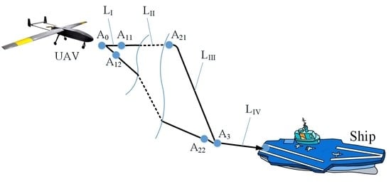
A typical approach landing trajectory between a common UAV and a vessel is shown in Figure 1. At the time t = 0 (starting of the approach maneuver), the UAV is at the point ${\mathit{A}}_0$, with coordinates $\left(\begin{array}{ccc}{x}_{A0}& y_{A0}& z_{A0}\end{array}\right)$, speed ${\mathit{V}}_A\left(t\right)$, and speed direction expressed as ${\mathit{\phi }}_{A0}\left(\begin{array}{cc}{\gamma }_{A0}& {\vartheta }_{A0}\end{array}\right)$. Similarly, at the time t = 0, the vessel carrying the land-based device is located at a point ${\mathit{B}}_0$, with coordinates $\left(\begin{array}{ccc}{x}_{B0}& y_{B0}& z_{B0}\end{array}\right)$, speed ${\mathit{V}}_B\left(t\right)$, and speed direction of ${\mathit{\phi }}_{B0}\left(\begin{array}{cc}{\gamma }_{B0}& {\vartheta }_{B0}\end{array}\right)$.

It is assumed that during the UAV landing approach, the mode of the UAV motion velocity vector is ${\mathit{V}}_A\left(t\right)$, the mode of the vessel motion velocity vector is ${\mathit{V}}_B\left(t\right)$, and the vessel motion velocity direction ${\mathit{\phi }}_{B0}$ are known constants. For the UAV landing time $t_B$, the predicted position of the vessel is ${\mathit{B}}_T\left(\begin{array}{ccc}{x}_{BT}& y_{BT}& z_{BT}\end{array}\right)$. At this time, the mode of the vessel’s motion velocity vector is constant ${\mathit{V}}_B$ with its direction ${\mathit{\phi }}_{B0}\left(\begin{array}{cc}{\gamma }_{B0}& {\vartheta }_{B0}\end{array}\right)$.

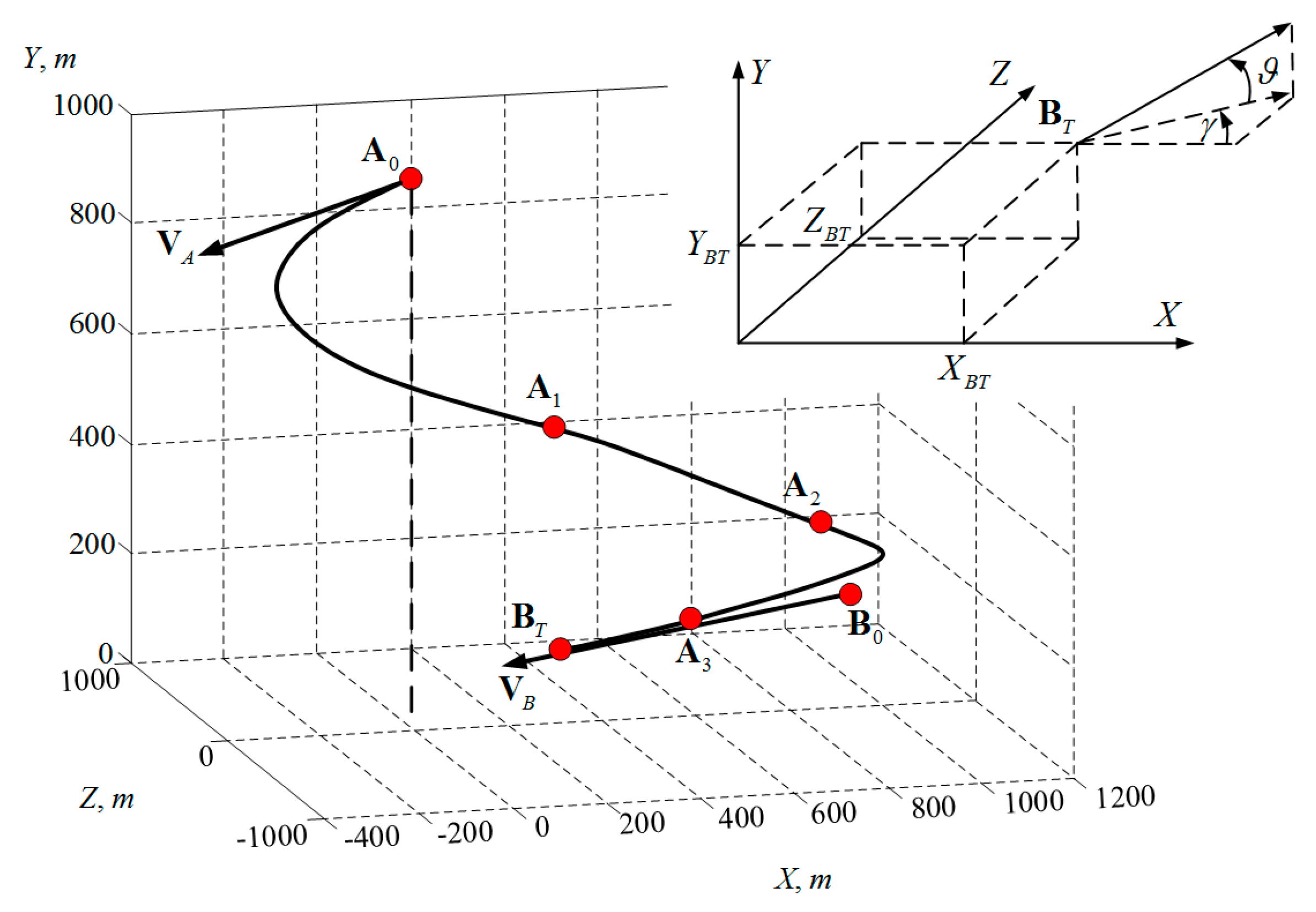
Assuming that the approach landing trajectory is in the plane $\left(\begin{array}{ccc}{\mathit{A}}_0& {\mathit{B}}_0& {\mathit{V}}_B\end{array}\right)$, and the origin of the initial coordinate system is selected at the point ${\mathit{B}}_0$, the coordinates of the point in the new obtained coordinate system are:

$$\{\begin{array}{c}{x}_1^{\prime }=x-x_{B0}\\ y_1^{\prime }=y-y_{B0}\\ z_1^{\prime }=z-z_{B0}\end{array}$$

(1)

where $x^{\prime }$, $y^{\prime }$, $z^{\prime }$, are the coordinates of the points in the new coordinate system, and $x$, $y$ $z$ are the coordinates of the points in the original coordinate system.

In order for the ship’s velocity vector to lie in the horizontal plane, the resulting coordinate system needs to be rotated by $-{\vartheta }_{B0}$ along the axis $x^{\prime }$. The new point coordinates in the resulting coordinate system are:

$$\{\begin{array}{c}{x}_2^{\prime }=x_1^{\prime }\\ y_2^{\prime }=-z_1^{\prime }sin\left(-{\vartheta }_{B0}\right)+y_1^{\prime }cos\left(-{\vartheta }_{B0}\right)\\ z_2^{\prime }=-z_1^{\prime }cos\left(-{\vartheta }_{B0}\right)+y_1^{\prime }sin\left(-{\vartheta }_{B0}\right)\end{array}$$

(2)

Finally, we rotate the obtained coordinate system along the axis $z^{\prime }$ by an angle:

$$\mathsf{\theta }=-\arctan \frac{\left(y_{2B0}^{\prime }-y_{2A0}^{\prime }\right)}{\left(x_{2B0}^{\prime }-x_{2A0}^{\prime }\right)}$$

The point coordinates in the resulting new coordinate system are:

$$\{\begin{array}{c}{x}^{\prime }=x_2^{\prime }cos\theta -y_2^{\prime }sin\theta \\ y^{\prime }=x_2^{\prime }sin\theta +y_2^{\prime }cos\theta \\ z^{\prime }=z_2^{\prime }\end{array}$$

(3)

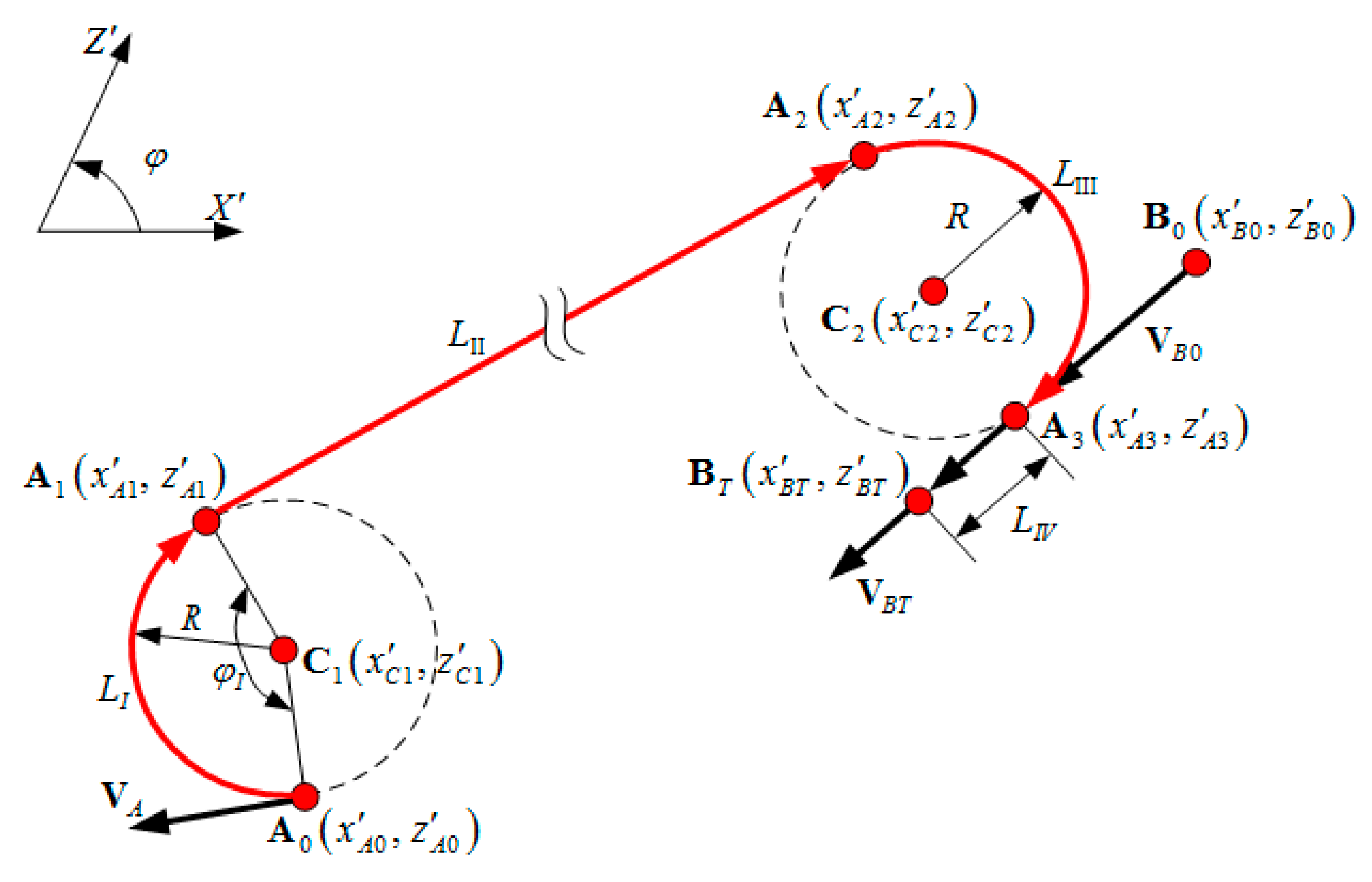
The complete approach trajectory from point ${\mathit{A}}_0$ to point ${\mathit{B}}_T$ in the resulting coordinate system will be in the plane $X^{\prime }{Z}^{\prime }$ (as shown in Figure 2).

The case shown in Figure 2 occurs when the pitch angle of both the UAV and the vessel is numerically close to each other. For example, when the UAV flies at a constant altitude before starting the approach landing decision. The sum direction of the axis $X^{\prime }$ and axis $Z^{\prime }$ and the positive direction of the angle in the plane $X^{\prime }{Z}^{\prime }$ are given in Figure 2.

In general, a landing trajectory approach consists of four feature segments. The first segment corresponds to the UAV landing turn, from the initial UAV position ${\mathit{A}}_0$ to point ${\mathit{A}}_1$ at the end of the turn. If the inertia of the UAV control system in the horizontal plane is neglected, then the maneuvering process can be considered to be done along the center of the circle ${\mathit{C}}_1\left(\begin{array}{cc}{x}_{C1}^{\prime }& y_{C1}^{\prime }\end{array}\right)$, with a minimum allowable turning radius $\mathrm{R}$ (in plane $X^{\prime }{Z}^{\prime }$). At this time:

$$\{\begin{array}{c}{x}_{C1}^{\prime }=x_{A0}^{\prime }+Rsin{\gamma }_{A0}\\ z_{C1}^{\prime }=z_{A0}^{\prime }-Rcos{\gamma }_{A0}\end{array}$$

(4)

The length of the first track is:

$$L_{\mathrm{I}}={\phi }_{\mathrm{I}}\mathrm{R}$$

(5)

of which the angular distance between ${\mathit{A}}_0$ and ${\mathit{A}}_1$ is ${\phi }_{\mathrm{I}}$, and $\mathrm{R}$ is the turning radius of the UAV. On this trajectory, the value of $\mathrm{R}$ is determined by the lateral overload allowable value $n_z$ [18]. For example, for $V_A=\left|{\mathit{V}}_A\left(t\right)\right|=60\mathrm{m}/\mathrm{s}$, $n_z=1$, we can get:

$$\mathrm{R}=\frac{V_A^2}{n_{z}g}\approx 360\mathrm{m}$$

In this case, the angular velocity of turn is:

$${\omega }_y=\frac{V_A}{R}=\frac{60}{360}=\frac{1}{6}\mathrm{rad}/\mathrm{s}\left({\omega }_y={10}^{\circ }/\mathrm{s}\right)$$

The second segment of the landing trajectory approach corresponds to a straight line segment, between the first maneuver completion point ${\mathit{A}}_1$ and the second maneuver start point ${\mathit{A}}_2$. The UAV enters the vessels navigation direction. The length of the trajectory is equal to the distance between the center of the first and second turns of the UAV, namely:

$$L_{\mathrm{II}}=\sqrt{{\left(x_{C2}-x_{C1}\right)}^2+{\left(z_{C2}-z_{C1}\right)}^2}$$

(6)

On this trajectory, the direction angle ${\phi }_{A2}$ of the UAV’s motion trajectory is calculated by:

$${\phi }_{A2}=\{\begin{array}{c}arctan\left(\frac{z_{C2}-z_{C1}}{x_{C2}-x_{C1}}\right), \left(x_{C2}-x_{C1}\ge 0\right)\\ \pi +arctan\left(\frac{z_{C2}-z_{C1}}{x_{C2}-x_{C1}}\right), \left(x_{C2}-x_{C1}<0\right)\end{array}$$

(7)

In the third segment, along the center of the circle ${\mathit{C}}_2$, the arc of radius $\mathrm{R}$ is flying from the point ${\mathit{A}}_2$ to the point ${\mathit{A}}_3$. At the point ${\mathit{A}}_3$, the UAV direction lies in the same direction of the ship carrying the landing device (ship). The length of the path is:

$$L_{\mathrm{III}}={\phi }_{\mathrm{III}}R$$

(8)

of which ${\phi }_{\mathrm{III}}$ refers to the angular distance between ${\mathit{A}}_2$ and ${\mathit{A}}_3$.

In the fourth section of the landing trajectory approach, the UAV moves along the direction of the vessel, making an approximate linear motion between the second maneuver completion point ${\mathit{A}}_3$ and the landing end point ${\mathit{B}}_T$. The length $L_{\mathrm{IV}}$ of the section is a constant value, about 200 to 300 m. The length of this passage is selected in advance based on the conditions that accurately guide the UAV to the landing device. On this path segment, a compensation of the calculated landing error, as well as a reduction in the UAV flight speed to the minimum required for landing, is achieved.

Assuming that $t_3$ is the time when the UAV ends its turn (return to point ${\mathit{A}}_3$), then, in general, the following equation can be obtained:

$${\mathit{A}}_3={\mathit{B}}_0+\underset{0}{\overset{t_3}{{\displaystyle \int }}}{\mathit{V}}_B\left(t\right)dt$$

(9)

For a specific uniform linear motion of the ship in the plane, we can get:

$$\{\begin{array}{c}{x}_{A3}^{\prime }=x_{B0}^{\prime }+V_B{t}_{3}cos{\gamma }_{B0}\\ z_{A3}^{\prime }=z_{B0}^{\prime }+V_B{t}_{3}sin{\gamma }_{B0}\end{array}$$

(10)

where the coordinates of the end point ${\mathit{B}}_T$, the UAV and the vessel are connected at this point:

$$\{\begin{array}{c}{x}_{BT}^{\prime }=x_{B0}^{\prime }+\left(V_B{t}_3+L_{\mathrm{IV}}\right)cos{\gamma }_{B0}\\ z_{BT}^{\prime }=z_{B0}^{\prime }+\left(V_B{t}_3+L_{\mathrm{IV}}\right)sin{\gamma }_{B0}\end{array}$$

(11)

After determining the coordinates of the point ${\mathit{A}}_3$, the coordinates of the turning circle center ${\mathit{C}}_2$ of the third segment of the landing trajectory can be obtained with the following relationship:

$$\{\begin{array}{c}{x}_{C2}^{\prime }=x_{A3}^{\prime }+Rsin{\gamma }_{BT}\\ z_{C2}^{\prime }=z_{A3}^{\prime }+Rcos{\gamma }_{BT}\end{array}$$

(12)

In addition, according to Equation (7), the angle ${\phi }_{A2}$ can be obtained, and then the coordinates of the point ${\mathit{A}}_1$ and ${\mathit{A}}_2$ are obtained as follows:

$$\{\begin{array}{c}{x}_{A1}^{\prime }=x_{C1}^{\prime }-Rsin{\phi }_{A2}\\ z_{A1}^{\prime }=z_{C1}^{\prime }+Rcos{\phi }_{A2}\\ \begin{array}{c}{x}_{A2}^{\prime }=x_{C2}^{\prime }-Rsin{\phi }_{A2}\\ z_{A2}^{\prime }=z_{C2}^{\prime }+Rcos{\phi }_{A2}\end{array}\end{array}$$

(13)

The difficulty in solving Equations (4)–(13) is that the value $t_3$ is indeterminate. To this end, this paper proposes an iterative method to determine the values of $t_3$. For the approximation of $t_3$, we can use:

$$t_3\left(i=1\right)=\frac{\sqrt{{\left(x_{B0}-x_{A0}\right)}^2+{\left(z_{B0}-z_{A0}\right)}^2}}{\left(V_A\pm V_B\right)}+\frac{\pi R}{V_A}$$

(14)

where if the UAV and the vessel are facing each other, the symbol “$+$” is selected, but if not, the symbol “$-$” is selected. In formula (14), the angle between the UAV flight speed vector and the ship’s navigation speed vector cannot be equal to 90°.

The error $\Delta \mathrm{t}$ of a single approximation does not exceed the following value:

$$\Delta \mathrm{t}=\frac{\pi R}{V_A}$$

(15)

Within the interval $\left[t_3\left(i=1\right)-\Delta t, t_3\left(i=1\right)+\Delta t\right]$, the value $t_3$ is searched and determined by the binary method. The search termination condition is:

$$\left|{\mathit{A}}_{2\mathrm{II}}\left(t_3\left(i\right)\right)-{\mathit{A}}_{2\mathrm{III}}\left(t_3\left(i\right)\right)\right|<\epsilon$$

(16)

where $\epsilon$—sets the coordinate error of point ${\mathit{A}}_2$ in the track segment $L_{\mathrm{II}}-A_{2\mathrm{II}}\left(t_3\left(i\right)\right)$ and $L_{\mathrm{III}}-A_{2\mathrm{III}}\left(t_3\left(i\right)\right)$. The value $\epsilon$ is determined by the accuracy of the actual landing trajectory approach, and in this paper is selected as $\epsilon \le 10\mathrm{m}$. ${\mathit{A}}_{2\mathrm{II}}$ refers to the point at the end of the left side trajectory of point ${\mathit{A}}_2$ (the second trajectory); ${\mathit{A}}_{2\mathrm{III}}$ refers to the point at the end of the right side trajectory of point ${\mathit{A}}_2$ (the third trajectory).

When the vessel is cruising at a constant speed, at ${\phi }_{A2}\left(t_3\left(i\right)\right)$ according to Equation (7), the coordinates of the point ${\mathit{A}}_{2\mathrm{II}}$ are:

$$\{\begin{array}{c}{x}_{2\mathrm{II}}^{\prime }=x_{C1}^{\prime }-Rsin{\phi }_{A2}\left(t_3\left(i\right)\right)+L_{\mathrm{II}}cos{\phi }_{A2}\left(t_3\left(i\right)\right)\\ z_{2\mathrm{II}}^{\prime }=z_{C1}^{\prime }+Rcos{\phi }_{A2}\left(t_3\left(i\right)\right)+L_{\mathrm{II}}sin{\phi }_{A2}\left(t_3\left(i\right)\right)\end{array}$$

(17)

With the coordinates of the point ${\mathit{A}}_{2\mathrm{III}}$ being:

$$\{\begin{array}{c}{x}_{2\mathrm{III}}^{\prime }=x_{C2}^{\prime }-Rsin{\phi }_{A2}\left(t_3\left(i\right)\right)\\ z_{2\mathrm{III}}^{\prime }=z_{C2}^{\prime }+Rcos{\phi }_{A2}\left(t_3\left(i\right)\right)\end{array}$$

(18)

After the value $t_3$ is determined, the total length $L$ of the approach landing trajectory is determined by the sum of the length of the four-part trajectory segments:

$$L=L_{\mathrm{I}}+L_{\mathrm{II}}+L_{\mathrm{III}}+L_{\mathrm{IV}}$$

(19)

By calculating the length $L$ of the shortest approach landing trajectory in real time, according to Equation (19), we can control the likelihood of the UAV returning to the landing device on the vessel. If the remaining fuel amount of the aircraft is less than the fuel amount $M_{KP}$ required to return to the vessel, then the UAV must perform a return maneuver. Among them, $M_{KP}$ is determined according to Equation (20).

$$M_{KP}=L{m}_L$$

(20)

where $m_L$ refers to the amount of fuel consumed by the drone unit path.

It is worth noting that, if $L_{\mathrm{II}}\ge L_{\mathrm{I}}+L_{\mathrm{III}}+L_{\mathrm{IV}}$, the approximate calculation Formula (21) can be used to replace the exact calculation formula of the landing trajectory approach $L$ (14).

$$L=\frac{\sqrt{{\left(x_{B0}-x_{A0}\right)}^2+{\left(z_{B0}-z_{A0}\right)}^2}}{\left(1\pm \frac{V_B}{V_A}\right)}+2\pi R$$

(21)

where $+$ or $-$ is used when the UAV and the vessel are facing or are opposite each other, respectively.

The ratio of average speeds is defined by:

$$\frac{V_B}{V_A}=\frac{{{\displaystyle \int }}_0^{t_3}\left|{\mathit{V}}_B\left(t\right)\right|dt}{{{\displaystyle \int }}_0^{t_3}\left|{\mathit{V}}_A\left(t\right)\right|dt}$$

(22)

In order to estimate the error of the approximate calculation Formula (21), it is preferable to perform a more accurate calculation of the average speed ratio.

Based on the above-mentioned transformation relationship among coordinate systems, the coordinates in the reference coordinate system are calculated according to the coordinates ${\mathit{C}}_1$, ${\mathit{C}}_2$, ${\mathit{A}}_1$, ${\mathit{A}}_2$, ${\mathit{A}}_3$ of the approaching landing trajectory feature points in the new coordinate system. At this time, the transformation order is reversed, and the sign of the corner of the coordinate system and the sign of the displacement of the coordinate origin are also opposite.

The research work in this paper is applicable in an ideal UAV control system, regardless of the inertia of the UAV control system. The actual approach landing trajectory between the UAV and the vessel can be determined by simulating the movement of the UAV along with an ideal landing trajectory.

3. Initial Error Estimation of an UAV Autonomous Guidance System

3.1. Optimal Approach Landing Trajectory Simulation between an UAV and a Vessel

For each landing trajectory (I, II, and III), the calculation of the landing trajectory coordinates between the UAV and the vessel is independent of each other. For the trajectory I, the $i$ point coordinates $\left(x_1\left(i\right), z_1\left(i\right)\right)$ of the approach landing trajectory are calculated according to the iterative Formula (23).

$$\{\begin{array}{c}{x}_1\left(i\right)=x_{C1}+Rcos\phi \left(i\right)\\ z_1\left(i\right)=z_{C1}+Rsin\phi \left(i\right)\end{array}$$

(23)

where the value $\mathsf{\phi }\left(i\right)=\mathsf{\phi }\left(i-1\right)+\Delta \phi , i=2, 3, \dots$, $\Delta \mathsf{\phi }={\omega }_y\Delta t$, $\Delta t$ is set. $\mathsf{\phi }\left(0\right)$ is the initial angle value of turning circular arc rotated according to the UAV speed vector.

If the descent angle in the vertical plane ${\vartheta }_{tr}$ is constant, then it can be defined as the ratio of the height difference between the UAV and the vessel to the horizontal distance between the UAV and the vessel:

$$\tan \left({\vartheta }_{tr}\right)=\frac{y_{A3}-y_{A0}}{\sqrt{{\left(x_{A3}-x_{A0}\right)}^2+{\left(z_{A3}-z_{A0}\right)}^2}}$$

(24)

For each approach landing trajectory, the following relationship is used:

$$\{\begin{array}{c}{y}_{1,2,3}\left(i\right)=y_{1,2,3}\left(i-1\right)+\Delta y, i=2, 3, \dots \\ \Delta y=\sqrt{{\left(x_{1,2,3}\left(i\right)-x_{1,2,3}\left(i-1\right)\right)}^2+{\left(z_{1,2,3}\left(i\right)-z_{1,2,3}\left(i-1\right)\right)}^2}tan\left({\vartheta }_{tr}\right)\end{array}$$

(25)

The termination condition for the I approach landing trajectory is:

$$\frac{\left|x_1\left(i\right)-x_{A1}\right|+\left|z_1\left(i\right)-z_{A1}\right|}{2}\le \epsilon$$

(26)

using the $\epsilon$ given value. When the termination condition (26) is satisfied, the number $i_1$ of calculation points of the I landing trajectory is considered as $i_1=i$.

For the II (straight) landing trajectory, the coordinates $\left(x_2\left(i\right), z_2\left(i\right)\right)$ of the $i$ point of the approach landing trajectory are calculated according to the iteration Formula (27).

$$\{\begin{array}{c}{x}_2\left(i\right)=x_{A1}+i{V}_A\Delta tcos{\phi }_{A2}\\ z_2\left(i\right)=z_{A1}+i{V}_A\Delta tsin{\phi }_{A2}\end{array}$$

(27)

where $i=1,2,\dots$.

The termination condition for the approach landing trajectory II is:

$$\frac{\left|x_2\left(i\right)-x_{A2}\right|+\left|z_2\left(i\right)-z_{A2}\right|}{2}\le \epsilon$$

(28)

When the termination condition is met, the number of calculation points for the approach landing trajectory II is $i_2=i$.

The calculation of the coordinates $\left(x_3\left(i\right), z_3\left(i\right)\right)$ of landing trajectory III is similar to the calculation of the coordinates of landing trajectory I, and the number of points calculated on the path is $i_3$.

Similarly, the calculation of the coordinates $\left(x_4\left(i\right), z_4\left(i\right)\right)$ of landing trajectory IV is analogous to the calculation of the coordinates of landing trajectory II. Since the UAV flies to a fixed position of the landing device in a self-guided way on the trajectory IV, the trajectory IV is out of the scope of this paper. In summary, the feasibility of the UAV approaching landing trajectory studied in this paper is restricted by the landing trajectory III. The actual error of the trajectory III will determine the initial error of the UAV autonomous guidance system.

In this work, the complete approach landing trajectory coordinate array consists of the corresponding array of trajectory coordinates of each trajectory segment, namely: ${\mathit{A}}_{tr}=\left[{\mathit{A}}_1\left(1: i_1, 1:i_1\right), {\mathit{A}}_2\left(1: i_2, 1:i_2\right), {\mathit{A}}_3\left(1: i_3, 1:i_3\right)\right]$.

3.2. UAV Motion Simulation Based on Optimal Approach Landing Trajectory

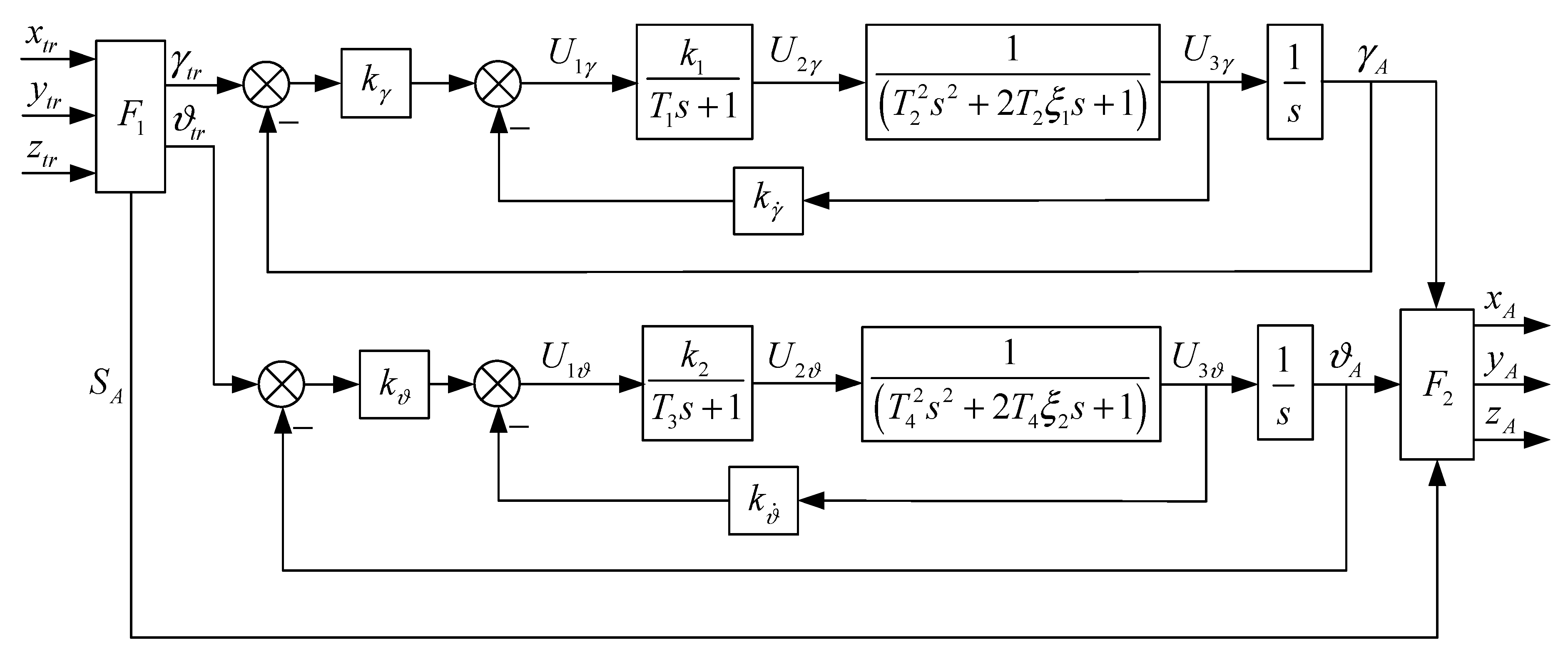
The dynamic structure of the UAV attitude control system in the horizontal and vertical planes is shown in Figure 3. The values $T_1$, $T_2$, $T_3$, and $T_4$ correspond to the time constant of the steering gear system and the aircraft; the ${\xi }_1$ and ${\xi }_2$ are the damping coefficients; with $k_1$, $k_2$, $k_{\gamma }$, $k_{\dot{\gamma }}$, $k_{\vartheta }$, $k_{\dot{\vartheta }}$, the track azimuth ${\gamma }_A$ and the track dip angle ${\vartheta }_A$ and its control loop transfer coefficient of rate of change.

In the coordinate converter $F_1$, the calculation formulas of the track azimuth ${\gamma }_{tr}$ and the track dip angle ${\vartheta }_{tr}$ of the UAV flight speed vector at the $i$ approach landing trajectory point are:

$$\{\begin{array}{c}{\gamma }_{tr}\left(i\right)=arctan\left(\frac{z_{tr}\left(i+1\right)-z_{tr}\left(i\right)}{x_{tr}\left(i+1\right)-x_{tr}\left(i\right)}\right)\\ {\vartheta }_{tr}\left(i\right)=arctan\left(\frac{y_{tr}\left(i+1\right)-y_{tr}\left(i\right)}{\sqrt{{\left(x_{tr}\left(i+1\right)-x_{tr}\left(i\right)\right)}^2+{\left(z_{tr}\left(i+1\right)-z_{tr}\left(i\right)\right)}^2}}\right)\end{array}$$

(29)

$$S_A\left(i\right)=\sqrt{{\left(x_{tr}\left(i+1\right)-x_{tr}\left(i\right)\right)}^2+{\left(y_{tr}\left(i+1\right)-y_{tr}\left(i\right)\right)}^2+{\left(z_{tr}\left(i+1\right)-z_{tr}\left(i\right)\right)}^2}$$

(30)

The integration step is defined as:

$$\Delta \mathrm{T}=\frac{S_A\left(i\right)}{V_A\left(i\right)}$$

(31)

In the transverse plane, the finite difference forms of the equation of motion of the UAV are:

$$\{\begin{array}{c}{\mathrm{U}}_{1\gamma }\left(i\right)=k_{\gamma }\left({\gamma }_{tr}\left(i\right)-{\gamma }_A\left(i-1\right)\right)-k_{\dot{\gamma }}{U}_{3\gamma }\left(i-1\right)\\ U_{2\gamma }\left(i\right)=U_{2\gamma }\left(i-1\right)+\frac{\left(k_1{U}_{1\gamma }\left(i-1\right)-U_{2\gamma }\left(i-1\right)\right)\Delta T}{T_1}\\ U_{3\gamma }^{\prime }\left(i\right)=U_{3\gamma }^{\prime }\left(i-1\right)+\frac{\left(U_{2\gamma }\left(i-1\right)-2T_2{\xi }_1{U}_{3\gamma }^{\prime }\left(i-1\right)-U_{3\gamma }\left(i-1\right)\right)\Delta T}{T_2^2}\\ U_{3\gamma }\left(i\right)=U_{3\gamma }\left(i-1\right)+U_{3\gamma }^{\prime }\left(i-1\right)\Delta T\\ {\gamma }_A\left(i\right)={\gamma }_A\left(i-1\right)+U_{3\gamma }^{\prime }\left(i-1\right)\Delta T\end{array}$$

(32)

In the longitudinal plane, the finite difference forms of the equation of the UAV motion are:

$$\{\begin{array}{c}{\mathrm{U}}_{1\vartheta }\left(i\right)=k_{\vartheta }\left({\vartheta }_{tr}\left(i\right)-{\vartheta }_A\left(i-1\right)\right)-k_{\dot{\vartheta }}{U}_{3\vartheta }\left(i-1\right)\\ U_{2\vartheta }\left(i\right)=U_{2\vartheta }\left(i-1\right)+\frac{\left(k_2{U}_{1\vartheta }\left(i-1\right)-U_{2\vartheta }\left(i-1\right)\right)\Delta T}{T_3}\\ U_{3\vartheta }^{\prime }\left(i\right)=U_{3\vartheta }^{\prime }\left(i-1\right)+\frac{\left(U_{2\vartheta }\left(i-1\right)-2T_2{\xi }_2{U}_{3\vartheta }^{\prime }\left(i-1\right)-U_{3\vartheta }\left(i-1\right)\right)\Delta T}{T_4^2}\\ U_{3\vartheta }\left(i\right)=U_{3\vartheta }\left(i-1\right)+U_{3\vartheta }^{\prime }\left(i-1\right)\Delta T\\ {\vartheta }_A\left(i\right)={\vartheta }_A\left(i-1\right)+U_{3\vartheta }^{\prime }\left(i-1\right)\Delta T\end{array}$$

(33)

After processing of the track azimuth ${\gamma }_A$ and track dip angle ${\vartheta }_A$ of the UAV flight speed vector by the coordinate converter $F_2$, the finite difference forms of the UAV’s centroid coordinates are as follows:

$$\{\begin{array}{c}{x}_A\left(i\right)=x_A\left(i-1\right)+S_A\left(i\right)cos{\gamma }_A\left(i\right)\\ y_A\left(i\right)=y_A\left(i-1\right)+S_A\left(i\right)cos{\vartheta }_A\left(i\right)\\ z_A\left(i\right)=z_A\left(i-1\right)+S_A\left(i\right)sin{\gamma }_A\left(i\right)\end{array}$$

(34)

In the design of the control system, the transmission azimuth loop transfer coefficient $\left(k_{\gamma }, k_{\dot{\gamma }}\right)$ and the track pitch loop transfer coefficient $\left(k_{\vartheta }, k_{\dot{\vartheta }}\right)$ must be carefully selected to ensure the stability margin and the quality of the transition process. Since the inertia of the control object is large, there is a distinct dynamic error.

For our simulation we used the following parameters: $T_1=T_3=0.3 \mathrm{s}$, $T_2=0.8 \mathrm{s}$, $T_4=0.5 \mathrm{s}$, $k_1=30$, $k_2=50$, ${\xi }_1={\xi }_2=1$, $k_{\gamma }=k_{\vartheta }=1$, $k_{\dot{\gamma }}=k_{\dot{\vartheta }}=0.2 \mathrm{s}$. UAV speed vector initial track azimuth ${\gamma }_{A0}={120}^{\circ }$, vessel speed vector initial track inclination ${\vartheta }_{A0}={20}^{\circ }$, UAV minimum turning radius $\mathrm{R}=720\mathrm{m}$, UAV flight speed $40 \mathrm{m}/\mathrm{s}$, vessel sailing speed $10 \mathrm{m}/\mathrm{s}$, landing position $x_{A0}=0 \mathrm{m}$, $z_{A0}=0 \mathrm{m}$, $y_{A0}=1000 \mathrm{m}$ of UAV at the initial landing time, Landing position $x_{B0}=2500 \mathrm{m}$, $z_{B0}=2500 \mathrm{m}$, $y_{B0}=0 \mathrm{m}$ of the vessel at the initial landing moment, the sampling period $\Delta \mathrm{T}=0.01\mathrm{s}$.

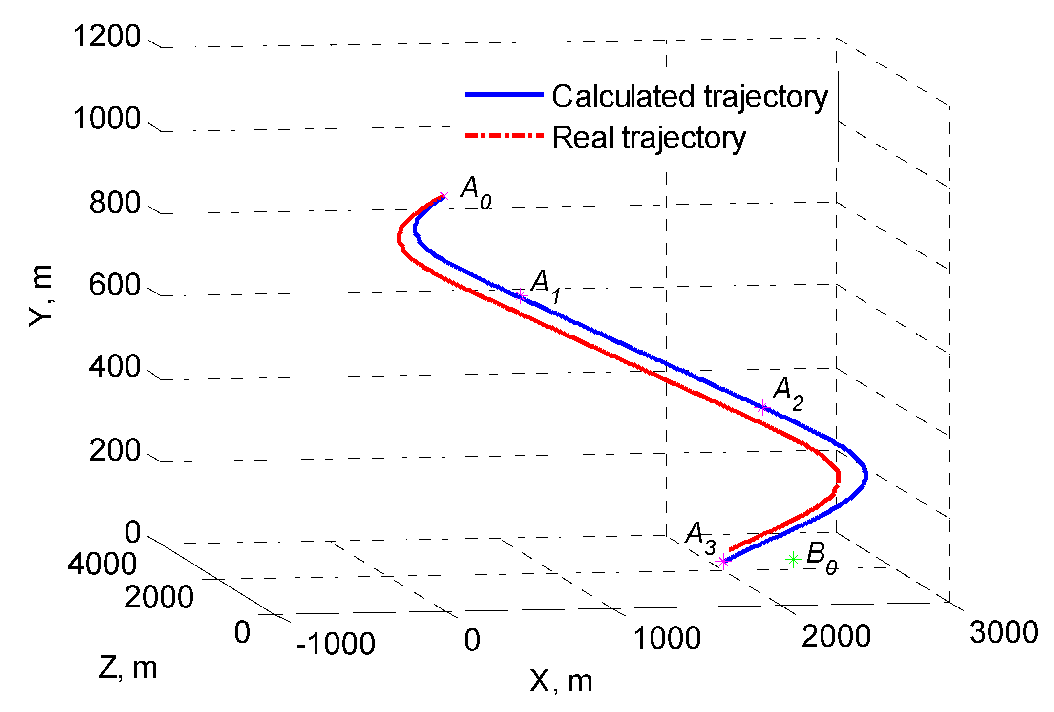
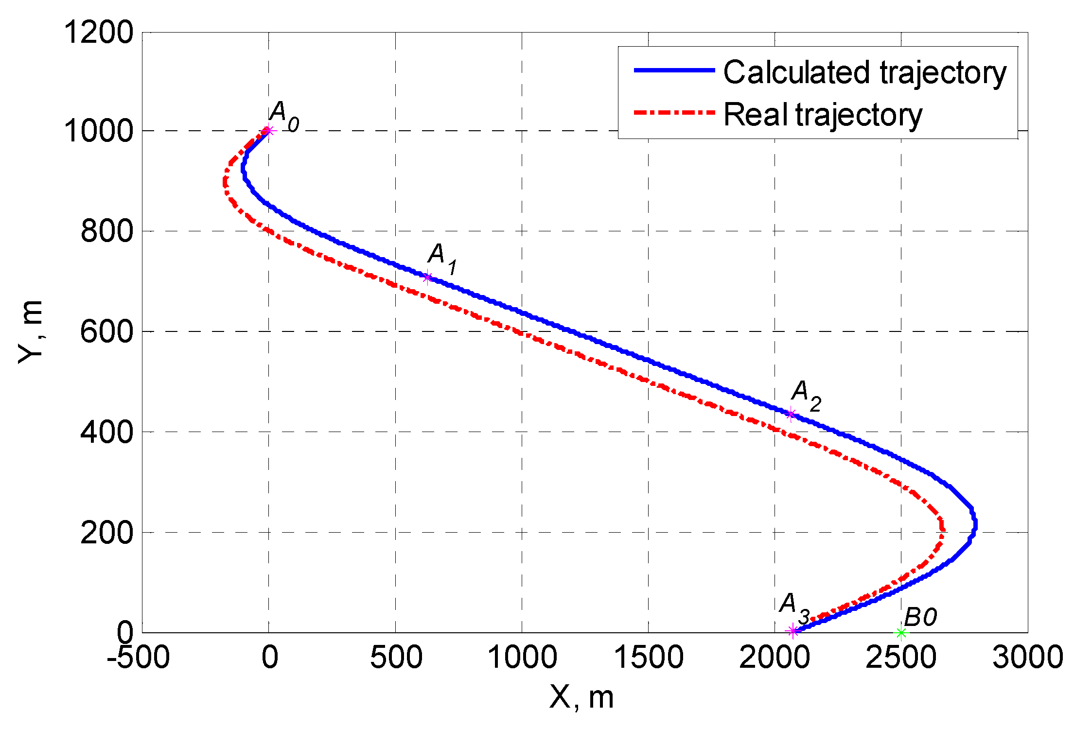
The spatial path of the UAV trajectory (from point ${\mathit{A}}_0$ to point ${\mathit{A}}_3$) is shown in Figure 4, and the projection in the vertical plane $XY$ is shown in Figure 5. The projection in the horizontal plane $XZ$ is shown in Figure 6.

In Figure 4, Figure 5 and Figure 6, the blue solid line indicates the calculated optimal approach landing trajectory, and the red dashed line indicates the actual approach landing trajectory. At the point ${\mathit{A}}_3$, the coordinate deviation between the actual trajectory of the UAV and the optimal calculated trajectory is $\Delta X=33.7\mathrm{m}$, $\Delta Z=34.45\mathrm{m}$, and the total error $\Delta S=53.8\mathrm{m}$. Such deviations can seriously affect the autonomous guidance of the last segment of the landing trajectory since, in many cases, directing the UAV to the autonomous guidance area of the landing device is an intractable task.

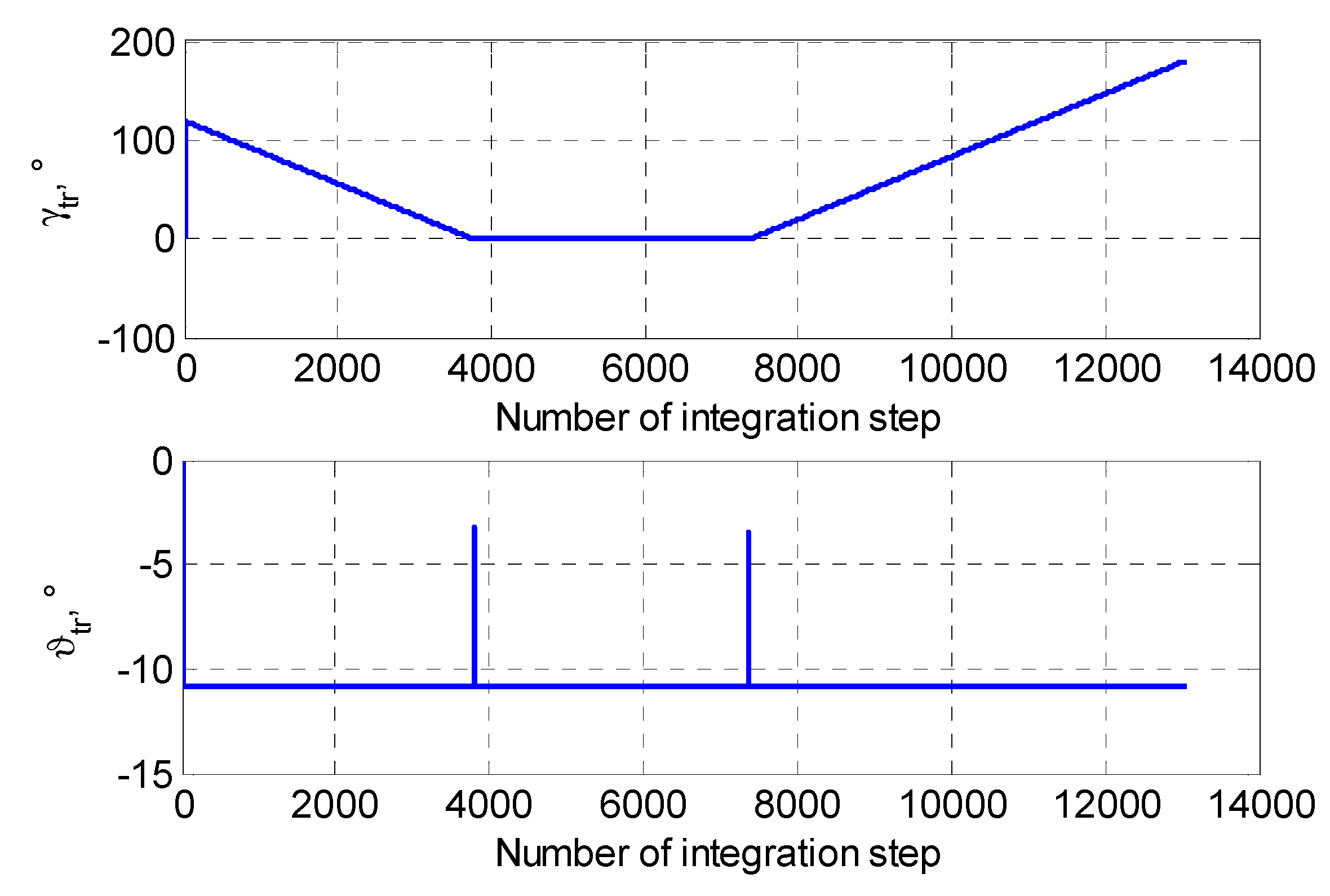
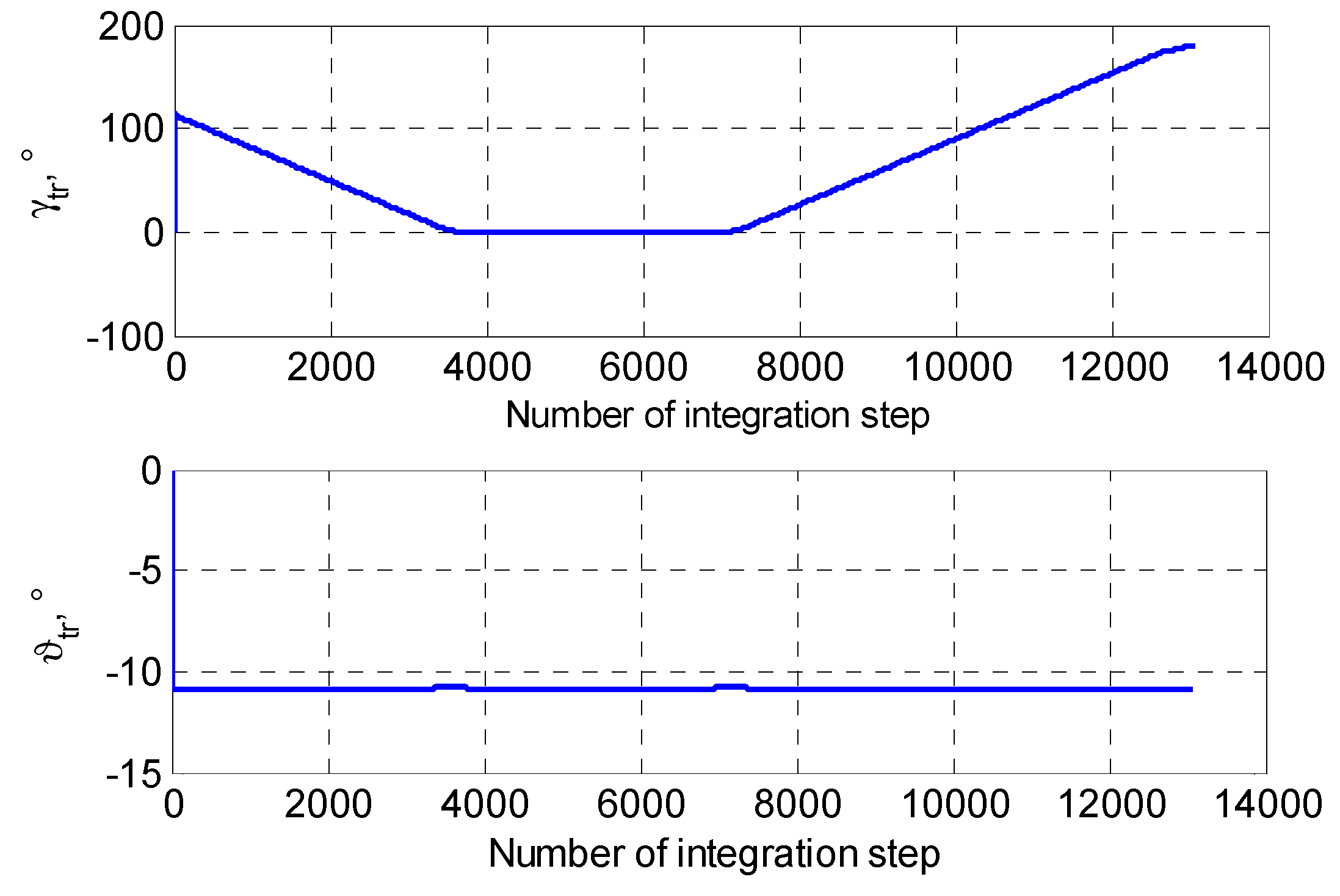
At the $i$$i$ calculation point of the approaching landing trajectory between the UAV and the vessel, the direction angle ${\gamma }_{tr}$ and dip angle ${\vartheta }_{tr}$ of the UAV flight speed vector are shown in Figure 7.

As shown in the simulation results of Figure 7 during the complete approach landing trajectory calculation, the direction angle ${\gamma }_{tr}$ of the UAV flight speed vector changes more smoothly, while the dip angle ${\vartheta }_{tr}$ of the UAV flight speed vector changes more sharply with a step change occurring at the points ${\mathit{A}}_1$ and ${\mathit{A}}_2$ of the approach landing trajectory. This step change is not conducive to an optimal UAV landing trajectory during actual flight.

4. Improving the Accuracy of the Optimal Approach Landing Trajectory

In order to improve the accuracy of the optimal approach landing trajectory between UAV and vessel, we introduce the pre-position n in the calculation formula of the direction angle ${\gamma }_A$ and the dip angle ${\vartheta }_A$ of the UAV flight speed vector. More precisely, we replace Equation (29) with Equation (35) and calculate the direction angle ${\gamma }_A$ and dip angle ${\vartheta }_A$ as follows:

$$\{\begin{array}{c}{\gamma }_{tr}\left(i\right)=arctan\left(\frac{z_{tr}\left(i+n\right)-z_{tr}\left(i\right)}{x_{tr}\left(i+n\right)-x_{tr}\left(i\right)}\right)\\ {\vartheta }_{tr}\left(i\right)=arctan\left(\frac{y_{tr}\left(i+n\right)-y_{tr}\left(i\right)}{\sqrt{{\left(x_{tr}\left(i+n\right)-x_{tr}\left(i\right)\right)}^2+{\left(z_{tr}\left(i+n\right)-z_{tr}\left(i\right)\right)}^2}}\right)\end{array}$$

(35)

with n denoting the initial lead steps.

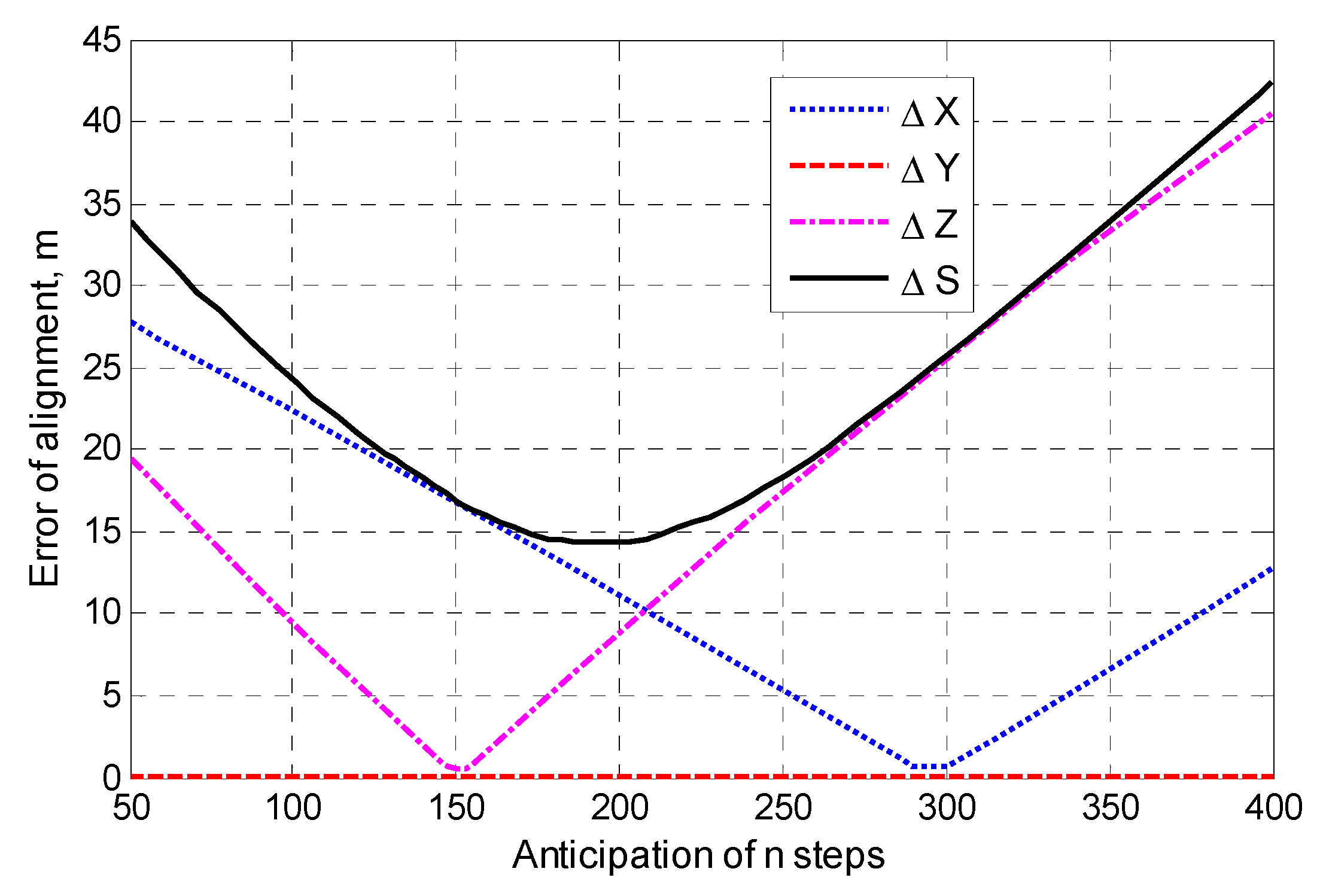
By selecting the optimal value of the initial lead steps n, the guidance error of the UAV’s flying to point ${\mathit{A}}_3$ can be greatly reduced. For the control system with the above parameters, different pre-step values are evaluated, and the coordinate deviation error $\Delta X$, $\Delta Y$, $\Delta Z$ and the total error $\Delta S=\sqrt{\Delta X^2+\Delta Y^2+\Delta Z^2}$ between the UAV actual trajectory and the optimal calculated trajectory at the point ${\mathit{A}}_3$ are shown in Figure 8.

In Figure 8, $\Delta Y=0$ is achieved by artificial compensation for systematic errors of $\Delta Y=14 \mathrm{m}$. From the simulation results shown in Figure 8, it can be concluded that the optimal value of the initial lead is $n=187$. At this value, the total error between the actual UAV approach landing trajectory and the vessel at the point ${\mathit{A}}_3$ is $\Delta S=14.2\mathrm{m}$ and the calculated optimal approach landing trajectory, which is compared with the total error when $n=1$, is reduced by nearly 3.5 times.

The direction angle ${\gamma }_{tr}$ and the dip angle ${\vartheta }_{tr}$ of the flight speed vector between the UAV and the vessel are shown in Figure 9.

From the simulation results shown in Figure 9, it can be seen that when the initial lead is $n=187$, the direction angle ${\gamma }_{tr}$ change process of the UAV flight speed vector almost sees the same trend compared with the results of Figure 7, showing a more gradual correction. By contrast, in the calculation process of the complete approach landing trajectory, the flight vector’s dip angle ${\vartheta }_{tr}$ changed significantly compared with the results of Figure 7, with the change process at the approach point ${\mathit{A}}_1$ and ${\mathit{A}}_2$ being smoother. This behavior is considered beneficial to an optimal UAV landing trajectory tracking planning during actual flight.

By introducing the initial lead in the control signal, it can be concluded that the UAV inertia can be compensated for a certain extent, assuring a more efficient approach landing trajectory.

5. Conclusions

Since vessels are in a state of constant motion, the conventional UAV landing plans are obviously not efficient for such moving platform landings. In this paper, a method for calculating the optimal approach landing trajectory between an UAV and a small vessel is proposed. Simulation results demonstrate the ineffectiveness of conventional algorithms, since they present the following shortcomings: (1) At the point ${\mathit{A}}_3$ of approaching the landing trajectory III, the error between the actual UAV landing trajectory and the calculated optimal landing trajectory is large, which seriously affects the autonomous guidance accuracy; (2) at the points ${\mathit{A}}_1$ and ${\mathit{A}}_2$ of the calculated optimal trajectory, a step change in the dip angle seriously affects the UAV’s tracking planning path.

In order to tackle the above two problems, the initial lead $n$ is introduced in the calculation formula of the direction angle ${\gamma }_A$ and dip angle ${\vartheta }_A$ of the UAV flight speed vector. Based on the performed simulation results, the introduction of the initial lead can effectively solve the above two problems and provide the optimal value of the initial lead.

In order to determine the initial error of the autonomous guidance segment, it is necessary to estimate the deviation of the calculated trajectory under the influence of the atmospheric random disturbance and the navigation system’s error. At the end of the uniform landing of the UAV near the point ${\mathit{A}}_3$, the UAV needs to keep a lower flight height in order to achieve a connection to the landing device.

References

- Zhao, F.; Xie, X.; Li, M. Mathematical Modeling for Optimal Selection of Maritime Patrol Ship Type. Navig. China 2016, 39, 50–54. [Google Scholar]
- Zhang, Y.L.; Wang, Y.Z.; Han, Z. Research on UAV landing based on FastSLAM algorithm. Electron. Opt. Control 2017, 24, 83–87. [Google Scholar]
- Kim, N.V.; Bodunkov, N.E.; Krylov, I.G.; Fedyaeva, E.A. Selecting a Flight Path of an UAV to the Ship in Preparation of Deck Landing. Indian J. Sci. Technol. 2016, 9. [Google Scholar] [CrossRef]
- Jin, W.; Li, P.; Li, Y.; Qiu, L. Restricted regions and main influence parameters for the takeoff and landing of carrier-based aircrafts. Chin. J. Ship Res. 2016, 11, 28–34. [Google Scholar]
- Frølich, M. Automatic Ship Landing System for Fixed-Wing UAV. Master’s Thesis, Department of Engineering Cybernetics, Norwegian University of Science and Technology, Trondheim, Norway, 2015. [Google Scholar]
- Nayak, G.C.; D’Souza, V. Optimized UAV flight mission planning using STK and A* algorithm. Int. J. Emerg. Technol. Eng. 2014, 1, 139–141. [Google Scholar]
- Gao, X.Z.; Hou, Z.X.; Zhu, X.F.; Zhang, J.Y.; Chen, X.Q. The shortest path planning for manoeuvres of UAV. Acta Polytech. Hung. 2013, 10, 221–239. [Google Scholar]
- Clark, S.; Goodrich, M.A. A hierarchical flight planner forsensor-driven UAV missions. In Proceedings of the 2013 IEEE RO-MAN: 22nd IEEE International Symposium on Robot and Human Interactive Communication, Gyeongju, Korea, 26–29 August 2013; IEEE: Piscataway, NJ, USA, 2013; pp. 509–514. [Google Scholar]
- Filippis, L.D. Advanced Path Planning and Collision Avoidance Algorithms for UAVs. Ph.D. Thesis, Polytechnic University of Turin, Turin, Italy, 2012. Available online: http://porto.polito.it/2497102/ (accessed on 26 July 2016).
- Forsmo, E.J. Optimal Path Planning for Unmanned Aerial Systems. Master’s Thesis, Department of Engineering Cybernetics, Norwegian University of Science and Technology, Trondheim, Norway, 2012. [Google Scholar]
- Abramov, N.S.; Makarov, D.A.; Khachumov, M.V. Controlling Flight Vehicle Spatial Motion along a Given Route. Autom. Remote Control 2015, 76, 1070–1080. [Google Scholar] [CrossRef]
- Feng, Y.; Zhang, C.; Baek, S.; Rawashdeh, S.; Mohammadi, A. Autonomous Landing of a UAV on a Moving Platform Using Model Predictive Control. Drones 2018, 2, 34. [Google Scholar] [CrossRef]
- Sánchez, L.; José, L.; Saripalli, S.; Campoy, P.; Pestana, J.; Fu, C. Toward Visual Autonomous Ship Board Landing of a VTOL UAV. J. Intell. Robot. Syst. 2014, 74, 113–127. [Google Scholar] [CrossRef]
- Kai, W.; Chunzhen, S.; Yi, J. Research on Adaptive Guidance Technology of UAV Ship Landing System Based on Net Recovery. Procedia Eng. 2015, 99, 1027–1034. [Google Scholar] [CrossRef] [Green Version]
- Wang, L.; Bai, X. Quadrotor Autonomous Approaching and Landing on a Vessel Deck. J. Intell. Robot. Syst. 2018, 92, 125–143. [Google Scholar] [CrossRef]
- Moriarty, P.; Sheehy, R.; Doody, P. Neural networks to aid the autonomous landing of a UAV on a ship. In Proceedings of the Signals & Systems Conference, Killarney, Ireland, 20–21 June 2017. [Google Scholar]
- Brittany, A. Roston.DARPA SideArm Prototype Snags Drones out of the Air. Available online: https://www.slashgear.com/darpa-sidearm-prototype-snags-drones-out-of-the-air-06474053/ (accessed on 6 February 2017).
- Sun, M.; Shi, J. Real-time path planning algorithm for unmanned aerial vehicles in threatening environment. J. Comput. Appl. 2009, 29, 1840–1842. [Google Scholar]
Figure 1.
Approach trajectory between an UAV and a vessel.
Figure 2.
Characteristic approach trajectory of an UAV and a vessel.
Figure 3.
Structurally-dynamic scheme of UAV control system for angle in horizontal and vertical planes.
Figure 4.
Space motion trajectory of the UAV.
Figure 5.
Projection of the space motion trajectory of the UAV in the vertical plane .
Figure 6.
Projection of the space motion trajectory of the UAV in the horizontal plane .
Figure 7.
Direction angle and dip angle of the UAV flight speed vector.
Figure 8.
The relationship between the error , , , and the initial lead steps n.
Figure 9.
© 2019 by the authors. Licensee MDPI, Basel, Switzerland. This article is an open access article distributed under the terms and conditions of the Creative Commons Attribution (CC BY) license (http://creativecommons.org/licenses/by/4.0/).
Share and Cite
MDPI and ACS Style
Tan, L.; Wu, J.; Yang, X.; Song, S. Research on Optimal Landing Trajectory Planning Method between an UAV and a Moving Vessel. Appl. Sci. 2019, 9, 3708. https://doi.org/10.3390/app9183708
AMA Style
Tan L, Wu J, Yang X, Song S. Research on Optimal Landing Trajectory Planning Method between an UAV and a Moving Vessel. Applied Sciences. 2019; 9(18):3708. https://doi.org/10.3390/app9183708
Chicago/Turabian StyleTan, Liguo, Juncheng Wu, Xiaoyan Yang, and Senmin Song. 2019. "Research on Optimal Landing Trajectory Planning Method between an UAV and a Moving Vessel" Applied Sciences 9, no. 18: 3708. https://doi.org/10.3390/app9183708
Note that from the first issue of 2016, this journal uses article numbers instead of page numbers. See further details here.