Pricing Personal Data Based on Data Provenance

Abstract

Data have become an important asset. Mining the value contained in personal data, making personal data an exchangeable commodity, has become a hot spot of industry research. Then, how to price personal data reasonably becomes a problem we have to face. Based on previous research on data provenance, this paper proposes a novel minimum provenance pricing method, which is to price the minimum source tuple set that contributes to the query. Our pricing model first sets prices for source tuples according to their importance and then makes query pricing based on data provenance, which considers both the importance of the data itself and the relationships between the data. We design an exact algorithm that can calculate the exact price of a query in exponential complexity. Furthermore, we design an easy approximate algorithm, which can calculate the approximate price of the query in polynomial time. We instantiated our model with a select-joint query and a complex query and extensively evaluated its performances on two practical datasets. The experimental results show that our pricing model is feasible.

1. Introduction

Data have become an important asset, and how to explore the value of personal data has become a hot topic. The term “personal data” refers to personal privacy data generated in the daily life or work of individuals, and individuals have ownership of the data [1]. With the further development of the mobile Internet, personal data as a valuable asset are growing exponentially [2]. A much effort has been made to define computing and resource-based pricing models [3]. Moiso et al. [4] presented a user-centered model in which individuals can collect, manage, use, and share their own data to discover their potential value. Personal data have different values for different objects. For example, personal data have different values for data owners and data analysis institutions. In [5], an effective method was designed to explore this competitive benefit distribution. Ng et al. [6] turned individuals into providers and co-creators of data services and products in the economy. However, only recently, Koutris et al. [7] studied some major pricing models of current data trading services and found that buyers can only purchase data through volume or predefined views. In the study of pricing models, arbitrage-free is an important economic attribute, but many pricing models have arbitrage phenomenon. Here, arbitrage refers to the strategy adopted for the purchase of data for greater benefits. For instance, it is more expensive to issue a single query than to issue several and combine their results.

Because of the current data trading market, there is little transparency between buyers and sellers, resulting in uncertainty about how data are collected, how they are handled before sales, and how they are used after sales. This may be the competitive strategy of some institutions, but it prevents the healthy development of the data market and creates information asymmetry. Therefore, it is necessary to trace the source tuples that produce the query results, and data provenance is a good solution to this problem. In [8], a data provenance trust model was proposed to evaluate the reliability of data and data providers according to various factors affecting the reliability. Huang et al. [9] constructed a heterogeneous data source provenance model based on the origin and evolution of data sources. Xing et al. [10] believed data provenance can be used to track query results, audit cloud computing data, and interpret big data analysis output. In this paper, a pricing model with a tuple granularity is devised. The model leverages and extends the concept of data provenance, that is a set of source tuples that contributes to query results.

When designing a personal data pricing model based on data provenance, there will be three difficulties. The first major difficulty is how can source tuples that contribute to query results be compensated reasonably. Furthermore, personal data have different values for data owners and data analysis institutions.

The second difficulty concerns designing a robust personal data pricing mechanism. The current personal data pricing mechanism is very simple, that is buyers can only choose explicit views, and each view has a specific price. Buyers can only purchase data through data volume or predefined views. The complex arbitrage behavior brings great challenges to the design of the pricing model.

The third difficulty is how to calculate the exact price of the query in an acceptable time. Personal data can be viewed as an information commodity with significant original investment costs, but the marginal cost of copying is negligible. As a result, value-based pricing models may be more suitable for personal data transactions.

The main contributions of this paper are as follows.

• A more rigorous personal data provenance model than the existing ones (e.g., [11,12,13]) is devised. In this model, even if a source tuple contributes to a query result multiple times, it is paid only once. A new provenance for a set of source tuples rather than a single source tuple is proposed.
• A creative pricing model is proposed. The pricing model includes two functions: price setting and pricing. A flexible set of pricing methods based on the p-norm [14] is proposed to provide the possibility of tuning and adapting to the pricing strategy for the data market. The pricing model satisfies three required properties: arbitrage-free, monotonic, and bounded.
• Our pricing model first sets prices for source tuples according to their importance and then makes query pricing based on data provenance, which considers both the importance of the data itself and the relationships between the data.
• An exact algorithm is used to calculate the exact price of a query with exponential complexity. Furthermore, an easy approximate algorithm that can calculate the approximate price of a query in polynomial time is devised.

The paper is organized in the following way. Section 2 introduces the existing relational data provenance semantics. Section 3 proposes a creative personal data pricing model that is based on minimal provenance. The exact algorithm and approximate algorithm are proposed to calculate the price of the query respectively in Section 4. Section 5 presents the experimental and evaluation results. Section 6 briefly reviews the related work. Section 7 concludes the paper.

2. Data Provenance

This section first reviews three forms of data provenance. The proposed model aims to pay a query, which is based on the source tuples contributing to the query result. Therefore, it is needed to track the source tuples given a query and its results.

Cheney et al. [15] stated that a relational database has three forms of “provenance”, which describes the relationship between source data and result data. “Where-provenance” is the first form, which has attribute-level granularity, indicating the origin of the attribute value of the source tuple contained in the query result. “Why-provenance” is the second form that explains why the result tuple returned is in the query result. “How-provenance” [13] is the third form that describes how source tuples form result tuples. The latter two forms have tuple level granularity.

The following is a sample relational database instance and query through Example 1.

Example 1.

Let I be a database instance, which is made up of relations R and S.

Table 1. Relation R.

ID	Name	Course No.
t1	John	00602001
t2	Tom	03310117
t3	James	04110235
t4	Tom	05110208

presents the contents of relation R, and

Table 2. Relation S.

ID	Course No.	Grade	Credit
t5	00602001	85	2
t6	00602001	90	2
t7	03310117	95	3
t8	05110208	75	1

presents the contents of relation S. Relation R records the course No. and the name of the student. For instance, the course No. is 00602001 for the student John. Relation S records the grade and the credit. For instance, consider Course No. 05110208, whose grade is 75 and whose credit is one. Each record in a relation is called a base tuple, for example relation R and relation S each contain four base tuples.

Suppose that student names need to be retrieved; then, the query (relational calculus) is $Q=\{<n>|\exists cn,\exists g,\exists c(R(n,cn)\bigwedge S(cn,g,c))\}$. Here, Q stands for query, R and S for relation, n for name attribute, $cn$ for course No. attribute, g for grade attribute, and c for credit attribute.

The query result is $Q(I)=\{<John>,<Tom>\}$. Here, Q represents the query, I represents the database instance, and $Q(I)$ represents the query result on database instance I.

Table 3. Provenances of each result tuple in Example 1.

Name	Why-Provenance [12]	Minimal Why-Provenance [11]
John	{$t_1$, $t_5$, $t_6$}	{{$t_1$,$t_5$},{$t_1,t_6$}}
Tom	{$t_2,t_4,t_7,t_8$}	{{$t_2,t_7$},{$t_4,t_8$}}
Name	How-Provenance [13]	Where-Provenance [11]
John	$t_1.t_5+t_1.t_6$	{$t_1.Name\}$
Tom	$t_2.t_7+t_4.t_8$	$\{t_2.Name\},\{t_4.Name\}$

records the various forms of provenance of the query results in Example 1. In the discussion below, Table 3 will be referenced.

2.1. Why-Provenance

The set of source tuples contributing to the result tuples is its why-provenance. Different versions of the why-provenance are due to different definitions of “contributing”. The source tuples sufficient to produce the result tuple are defined by the simplest one. Here, a result tuple is the set of tuples that make up the query results. In addition, the simplest refers to the minimum principle, which is the minimal set of tuples that can produce a result tuple. Many source tuples have no correlation with the presence of result tuples, resulting in a large number of such subsets.

The authors of [12] tried to filter the “irrelevant” source tuples to avoid this problem. They [12] considered each source tuple that contributed to a result tuple, and such a maximum set of source tuples is the why-provenance. However, the why-provenance computed by [12] will cause an issue, namely it will contain unnecessary base tuples.

Due to the why-provenance containing unnecessary source tuples, on the basis of a deterministic semi-structured data model and query language, the concept of why-provenance was defined in [11]. The definitions in [11] were adapted to the relational model and relational algebra by the authors of [15] (as shown below).

Definition 1.

Let I represent a database instance, Q represent a select-project-join-union query, and trepresent a result tuple in $Q(I)$. In accordance with Q and I, $Why(Q,I,t)$ denotes the set of why-provenances of t. Its definition is shown below:

• $Why({\sigma }_{\theta }(Q),I,t)=Why(Q,I,t),if$$\theta (t)$.
• $Why({\pi }_U(Q),I,t)$ = $\bigcup \{Why(Q,I,u)\mid u\in Q(I),t=u[U]\}$.
• $Why(Q_1\bowtie Q_2,I,t)$ = $Why(Q_1,I,t\left[U_1\right])⨆Why(Q_2,I,t\left[U_2\right])$.
• $Why(Q_1\bigcup Q_2,I,t)$ = $Why(Q_1,I,t)\bigcup Why(Q_2,I,t)$.

Here, selections ${\sigma }_{\theta }$ filter a relation by retaining tuples satisfying some predicate $\theta$. Projections ${\pi }_U(Q)$ replace each tuple t in a relation with $t\left[U\right]$, discarding any other fields. Join (or natural join) $Q_1\bowtie Q_2$ indicates a natural join between $Q_1$ and $Q_2$. Union $Q_1\bigcup Q_2$ represents the union of $Q_1$ and $Q_2$. ⨆ takes all the pairwise unions of two collections. That is, $A⨆B=\{a\bigcup b|a\in A,b\in B\}$.

Minimal why-provenance means that the subset of results produced is minimal. Thus, in some cases, there may exist several minimal why-provenances. There are two minimal why-provenances of $\langle John\rangle$: $\{t_1,t_5\}$ and $\{t_1,t_6\}$ in Table 3. Because $\{t_1,t_6\}$ generates $\langle John\rangle$ and none of its proper subsets can generate $\langle John\rangle$, it is a minimal why-provenance of $\langle John\rangle$.

2.2. Where-Provenance and How-Provenance

The where-provenance [11] of an attribute value in a result tuple consists of the attribute value of the source tuple. The where-provenance of $\langle John\rangle$ is $\{t_1.Name\}$ in Table 3, namely $\langle John\rangle$ comes from the “Name” attribute of $t_1$. The source tuples that contribute to a result tuple are obtained by the why-provenance. However, the why-provenance does not specify how to obtain the result tuple from the source tuples. Therefore, the how-provenance ([13]) is motivated. In Table 3, $t_1·t_5+t_1·t_6$ is the how-provenance of $\langle John\rangle$. Thus, we can produce $\langle John\rangle$ in two manners: the first method is joining $t_1$ and $t_5$, and the second method is joining $t_1$ and $t_6$. We can realize how source tuples contribute to the result $\langle John\rangle$ by this polynomial expression.

2.3. Problems with Current Provenance

The provenances of the above discussion are only applicable to the query result in individual source tuples. In this paper, we cannot use them for personal data pricing. If the above provenance method is used, each source tuple in the query result is priced separately and the prices added up. This causes the same source tuple to be charged multiple times in the database. Thus, it is necessary to ensure that even if each source tuple contributes to the query results many times, it can only be paid once. Therefore, it is necessary to design a more rigorous provenance model than existing ones (e.g., [11,12,13]). This is the focus of this paper.

According to [16], the existing pricing strategies include free use, usage-based pricing, packet pricing, fixed cost, two-part charging system, and freemium. The work in [17] argued that these pricing models assume that all source tuples are equivalent, which leads to an arbitrage situation. In [7], a query-based pricing model was proposed, which allows the seller to set a fixed price for the view. Minimum why-provenance was proposed in [11], but there may be several minimum why-provenances for the same query result tuple. The relational data pricing framework proposed in this paper differs from the previous work as follows. First of all, the work in [11] identified the provenance of a single source tuple. Different from [11], this paper identifies the provenance of a group of source tuples. Second, unlike in [7], pricing is based on view granularity, and our pricing model is based on tuple granularity. Finally, we propose an exact algorithm and an approximate algorithm to calculate the price of the query, which were not available in the previous work.

3. Pricing Data

This section first presents a creative pricing model, which includes two functions: price setting and pricing. Next, we define minimum provenance and the p-norm. Finally, we propose a pricing function based on contribution source tuples, which satisfies three important properties, i.e., monotonicity, boundedness, and arbitrage-freeness. The monotonicity ensures that the queries that use more source tuples have a higher price than those that use fewer source tuples. The boundedness guarantees that the price of any query cannot be higher than the price of the base tuple. The arbitrage-freeness is an important economic robustness guarantee against arbitrage. A valid pricing model must ensure its fairness, feasibility, and robustness through monotonicity, boundedness, and arbitrage-freeness, respectively.

3.1. Pricing Model

Two functions comprise our pricing model. The first function sets the price for the base tuple, and the second defines a price for the query.

Definition 2

(Price setting function [16]). Let I represent a database instance. A price setting function is $s_I$:$\mathbb{T}$→${\mathbb{R}}^{+}$, where $\mathbb{T}$ denotes the set of base tuples in I and ${\mathbb{R}}^{+}=[0,\infty )$.

Definition 3

(Pricing function [16]). Let I represent a database instance. A pricing function is $p_I:\mathbb{Q}\to {\mathbb{R}}^{+}$, where $\mathbb{Q}$ is the set of queries and ${\mathbb{R}}^{+}=[0,\infty )$.

3.2. Minimal Provenance

To prevent arbitrary queries from charging users for the entire database, you must consider enough source tuples to generate the given query results. However, there may be more than one minimum set of enough source tuples. This paper defines the provenance of query results as a whole, not as a single source tuple. In our pricing model, a tuple is paid at most once, regardless of how many times it contributes to the query result.

Definition 4

(Provenance [16]). Let $I,Q,Q(I)$ represent a database instance, a query, and the query results, respectively. A provenance of $Q(I)$ is a set of source tuples $T(T\subseteq I)$ so that $Q(I)\subseteq Q(T)$.

Definition 5

(Minimal provenance [16]). Let $V(Q,I)$ represent the minimum provenance set of $Q(I)$. $V(Q,I)$ is a provenance T of $Q(I)$, so that $\forall T^{\prime },T^{\prime }\subseteq T\Rightarrow T^{\prime }=T$, where $T^{\prime }$ is a provenance of $Q(I)$.

Example 2.

Based on Example 1, the query results $Q(I)$ have four minimal provenances, i.e., $T_1=\{t_1,t_2,t_5,t_7\},T_2=\{t_1,t_4,t_5,t_8\},T_3=\{t_1,t_2,t_6,t_7\}$, $T_4=\{t_1,t_4,t_6,t_8\}$.

Let us explain $T_1$. $T_1$ means the query result $\{<John>,<Tom>\}$ is produced by the set of source tuples $\{t_1,t_2,t_5,t_7\}$, but the query result $\{<John>,<Tom>\}$ cannot be produced by any subsets of $O_1$.

From Example 2, it can be observed that several $V(Q,I)$ exist in query result $Q(I)$. The following demonstrates that $V(Q,I)$ remains constant in the query rewriting.

Theorem 1.

$\forall I$, if $Q_1\equiv Q_2$, then $V(Q_1,I)=V(Q_2,I)$.

Proof. 

Suppose that $Q_1$, $Q_2$ are two equivalent queries: $Q_1\equiv Q_2$. $\forall I$, $Q_1(I)=Q_2(I)$.

Suppose that $\exists I^{\prime }$ such that $V(Q_1,I^{\prime })\ne V(Q_2,I^{\prime })$. Thus, at least one of the two sets contains some elements that the other does not. Suppose:

$$\exists T^{\ast }\in V(Q_1,I^{\prime })\wedge (\forall T_2\in V(Q_2,I^{\prime })\Rightarrow T^{\ast }\ne T_2)$$

(1)

Consider the following cases:

• $\exists T^{\prime }\in V(Q_2,I^{\prime })$ such that $T^{\ast }\subset T^{\prime }$. Build a database instance $I^{-}=T^{\ast }$. Because $T^{\ast }$ denotes a minimal provenance of $Q_1(I^{\prime })$,

  $$Q_1(I^{-})=Q_1(T^{\ast })=Q_1(I^{\prime })$$

  (2)
  Moreover, $T^{\ast }$ is not the provenance of $Q_2(I^{\prime })$. In that case, $T^{\prime }$ cannot be a minimal provenance,

  $$Q_2(I^{-})=Q_2(T^{\ast })⊉Q_2(I^{\prime })$$

  (3)
  Thus,

  $$Q_2(I^{-})\ne Q_2(I^{\prime })$$

  (4)
  Since $Q_1\equiv Q_2$, $Q_1(I^{\prime })=Q_2(I^{\prime })$ and $Q_1(I^{-})\ne Q_2(I^{\prime })$. This result violates $Q1\equiv Q2$.
• $\exists T^{\prime }\in V(Q_2,I^{\prime })$ such that $T^{\prime }\subset T^{\ast }$. Build a database instance $I^{-}=T^{\prime }$. Because $T^{\prime }$ denotes a minimal provenance of $Q_2(I^{\prime })$,

  $$Q_2(I^{-})=Q_2(T^{\prime })=Q_2(I^{\prime })$$

  (5)
  Moreover, $T^{\prime }$ is not the provenance of $Q_1(I^{\prime })$. In that case, $T^{\ast }$ cannot be a minimal provenance,

  $$Q_1(I^{-})=Q_1(T^{\prime })⊉Q_1(I^{\prime })$$

  (6)
  Thus,

  $$Q_1(I^{-})\ne Q_1(I^{\prime })$$

  (7)
  Since $Q_1\equiv Q_2$, $Q_1(I^{\prime })=Q_2(I^{\prime })$ and $Q_1(I^{-})\ne Q_2(I^{-})$. This result violates $Q1\equiv Q2$.
• $\nexists T^{\prime }\in V(Q_2,I^{\prime })$ so that $T^{\prime }\subset T^{\ast }$ or $T^{\ast }\subset T^{\prime }$. Build a database instance $I^{-}=T^{\ast }$. Because $T^{\ast }$ denotes a minimal provenance of $Q_1(I^{\prime })$,

  $$Q_1(I^{-})=Q_1(T^{\ast })=Q_1(I^{\prime })$$

  (8)
  Moreover, $T^{\ast }$ is not the provenance of $Q_2(I^{\prime })$ since $\forall T^{\prime }\in V(Q_2,I^{\prime })\Rightarrow T^{\ast }\ne T^{\prime }$. Additionally, $T^{\ast }$ cannot be a provenance of $Q_2(I^{\prime })$.
  Since $\nexists T^{\prime }\in V(Q_2,I^{\prime })$ such that $T^{\prime }\subset T^{\ast }$,

  $$Q_2(I^{-})=Q_2(T^{\ast })⊉Q_2(I^{\prime })$$

  (9)
  Thus,

  $$Q_2(I^{-})\ne Q_2(I^{\prime })$$

  (10)
  Since $Q_1\equiv Q_2$, $Q_1(I^{\prime })=Q_2(I^{\prime })$ and $Q_1(I^{-})\ne Q_2(I^{-})$. This result violates $Q1\equiv Q2$.

By the same logic, we can get that $\forall I^{\prime },V(Q_1,I^{\prime })=V(Q_2,I^{\prime })$. □

3.3. p-Norm

This section describes the p-norm and how it can be used for pricing adjustment. The p-norm [14] is a set of norms. The norm varies according to p. We can adjust the price according to the change of the p value.

Definition 6

(p-norm [16]). Let X represent a vector $(x_1,x_2,\dots ,x_n)$; for a real number $p\ge 1$, ${\parallel X\parallel }_p=({\sum }_{i=1}^n|x_i{{|}^p)}^{\frac{1}{p}}$ defines the p-norm of X.

When $p={1,\parallel X\parallel }_1={\sum }_{i=1}^n|x_i|$, it is the Manhattan norm of X. When $p={2,\parallel X\parallel }_2={({\sum }_{i=1}^n{x}_i^2)}^{\frac{1}{2}}$, it is the Euclidean norm of X. $p={\infty ,\parallel X\parallel }_{\infty }=max\{|x_1|,|x_2|,\dots ,|x_n|\}$. Similarly, by Definition 6, the p-norm can also be applied to the set.

Proposition 1

([16]). If $p\ge 1$ and $a\ge {0,\parallel X\parallel }_{p+a}\le {\parallel X\parallel }_p$.

Work of Buneman, et al. [11] was proven in Proposition 1. The value of the p-norm is inversely proportional to p, that is when p increases, the p-norm decreases.

Definition 7

([16]). Let $I,X$, and $s_I$ represent a database instance, a set of source tuples, and a price setting function, respectively. $X\subseteq I$. ${\parallel X\parallel }_p={({\sum }_{i=1}^n{s}_I{(t_i)}^p)}^{\frac{1}{p}}$ defines the price of X, where $t_i\in X$.

The p-norm becomes very effective when the data seller offers different discounts to different buyers. For an ordinary customer, p is equal to one, and for an important customer, p is greater than one. As the customer importance increases, so does the p value. This allows the data seller to adjust the size of the p value to provide different discounts to different customers. Therefore, Proposition 1 and Definition 7 can be used to set different prices for source tuples.

Proposition 2.

Assume that there are two sets $X_1$ and $X_2$. If $X_1\subseteq X_2,\mathrm{then}\parallel X_1{\parallel }_p\le {\parallel X_2\parallel }_p$.

Proposition 2 was proven in [14]. This proposition indicates that the more elements a set contains, the greater its p-norm value.

3.4. Pricing Function

The pricing function is used to price query so as to generate minimal provenance. First, define the minimum provenance to produce query results. Then, define several important properties that the pricing function must satisfy. Finally, a pricing function is proposed, and all defined properties are proven to be satisfied.

Definition 8

(Contribution tuples [16]). Let $I,Q,Q(I)$ represent a database instance, a query, and the query results, respectively. The minimal provenances of $Q(I)$, i.e., $V(Q,I)$ is the contribution tuples of $Q(I)$.

Property 1.

(Monotonicity) In fact, it is necessary to have such a property because it ensures that queries that use more source tuples have higher prices than those that use fewer source tuples. However, the implications of “using more source tuples” is uncertain when there are multiple methods for producing query results. If you use only a subset of all the source tuples that produce the results of query $Q_2$ to produce the results of query $Q_1$, you can assume that query $Q_2$ uses more source tuples than query $Q_1$ does.

Definition 9.

(Containment and equivalence) Let I represent a database instance and $Q_1$ and $Q_2$ be two queries. The sets of contribution tuples of $Q_1(I)$ and $Q_2(I)$ are denoted by $V(Q_1,I)$ and $V(Q_2,I)$, respectively. $Q_1$ is contained in $Q_2$ about I, namely $Q_1{\subseteq }_{C(I)}{Q}_2$, if and only if:

$$\forall T^{\prime }(T^{\prime }\in (V(Q_2,I)\Rightarrow \exists T(T\in (V(Q_1,I)\wedge T\subseteq T^{\prime }))))$$

(11)

$Q_1$ and $Q_2$ are equivalent, that is $Q_1{\equiv }_{C(I)}{Q}_2$, if and only if $Q_1{\subseteq }_{C(I)}{Q}_2$ and $Q_2{\subseteq }_{C(I)}{Q}_1$.

$Q_1{\subseteq }_C{Q}_2$, if and only if for any database instance $I,Q_1{\subseteq }_{C(I)}{Q}_2$.

$Q_1{\equiv }_C{Q}_2$, if and only if $Q_1{\subseteq }_C{Q}_2$ and $Q_2{\subseteq }_C{Q}_1$.

Example 3.

Let I represent a database instance and $Q_1$, $Q_2$, and $Q_3$ represent three queries. The sets of contributing tuples of $Q_1(I)$, $Q_2(I)$, and $Q_3(I)$ are denoted by $V(Q_1,I)$, $V(Q_2,I)$, and $V(Q_3,I$), respectively. Suppose that $V(Q_1,I)=\{T_1^1=\{t_1,t_2\},T_1^2=\{t_2,t_3\}\}$,$V(Q_2,I)=\{T_2^1=\{t_1,t_2,t_3\}\}$,$V(Q_3,I)=\{T_3^1=\{t_1,t_2\},T_3^2=\{t_1,t_3\}\}$.

$Q_1\subseteq Q_2$, because for $T_2^1$, there exists $T_1^1$ such that $T_1^1\subseteq T_2^1$. However, $Q_1{⊈}_{C(I)}{Q}_3$ because for $T_3^2$, $T_1^1⊈T_3^2$ and $T_1^2⊈T_3^2$.

For all the methods that produce the results of $Q_2$, we must ensure that the price of $Q_1$ is less than the price of $Q_2$, such that we can find the result of $Q_1$ in a less expensive manner.

Definition 10.

(Monotonicity) If given a database instance I, for any two queries $Q_1$ and $Q_2$, when $Q_1{\subseteq }_{C(I)}{Q}_2$, $p_I(Q_1)\le p_I(Q_2)$, then we can call the pricing function monotonic.

Property 2.

(Boundedness) The price of the base tuple involved in the query is an upper bound on the price of any query.

Definition 11.

(Boundedness) Let $S=\{t\in R|RQ\}$ represent the base tuples and $RQ$ represent the relation R involved in the query Q. If $\forall Q$, there exists ${\parallel S\parallel }_p\ge p_I(Q)$, then we say that the pricing function is bounded.

Lemma 1

([16]). If a pricing function is monotonic, then it is bounded.

Property 3.

(Arbitrage-freeness) The practice of taking full advantage of the price in multiple markets is called arbitrage. Consider the USA business dataset [7]: if p is the price for the entire dataset and $p_1,\dots ,p_{50}$ are the prices for the data in each of the 50 states, then a rational seller would ensure that $p<p_1+\dots +p_{50}$. Otherwise, no buyer would pay for the entire dataset, but would instead buy all 50 states’ datasets separately.

This paper addresses contributing tuples, thus the concept of arbitrage must be adapted for contributing tuples. For a query Q, its contribution tuples are $\{\{t_1,t_2,t_3\}\}$, and the price is p; for another query $Q_1$, its contribution tuples are $\{\{t_1,t_2\}\}$, and the price is $p_1$; and for a third query $Q_2$, its contribution tuples are $\{\{t_3,t_4\}\}$, and the price is $p_2$. The data seller must be sure that $p<p_1+p_2$. Otherwise, this results in the price of $\{\{t_1,t_2,t_3,t_4\}\}$ being lower than the price of $\{t_1,t_2,t_3\}$, which is unreasonable. In this situation, in which users can obtain contributing tuples, and if the query is not carefully defined, arbitrage can occur.

We have to avoid arbitrage, and we will formally define arbitrage-freeness.

Definition 12.

(Arbitrage-freeness) A pricing function is arbitrage-free if:

$$(\forall S(S=\bigcup _{1\le i\le m}{T}_{k_i}^i(T_{k_i}^i\in V(Q_i,I))\Rightarrow \exists T(T\in V(Q,I)\wedge T\subseteq S)))$$

(12)

${\sum }_i{p}_I(Q_i)\ge p_I(Q)$ holds.

Example 4.

Suppose that $V(Q_1,I)=\{T_1^1=\{t_1,t_2\},T_1^2=\{t_2,t_3\}\}$, $V(Q_2,I)=\{T_2^1=\{t_2,t_4\},T_2^2=\{t_1,t_4\}\}$, and $V(Q,I)=\{T^1=\{t_1,t_2\},T^2=\{t_2,t_3\},T^3=\{t_1,t_4\}\}$.

For $T_1^1\bigcup T_2^1=\{t_1,t_2,t_4\}$, there exists $T^1\subseteq T_1^1\bigcup T_2^1$.

For $T_1^2\bigcup T_2^1=\{t_2,t_3,t_4\}$, there exists $T^2\subseteq T_1^2\bigcup T_2^1$.

For $T_1^1\bigcup T_2^2=\{t_1,t_2,t_4\}$, there exists $T^1\subseteq T_1^1\bigcup T_2^2$.

For $T_1^2\bigcup T_2^2=\{t_1,t_2,t_3,t_4\}$, there exists $T^1\subseteq T_1^2\bigcup T_2^2$.

If $p_I(Q_1)+p_I(Q_2)\ge p_I(Q)$, then this pricing function is arbitrage-free.

Definition 13

(Price of a query [16]). The price of the least expensive minimal provenance of $Q(I)$ defines the price of a query Q in a database instance I:

$$P_I(Q)=\underset{T\in V(Q,I)}{min}{\parallel T\parallel }_p$$

(13)

Theorem 2

([16]). The pricing function in Definition 13 satisfies the following properties:

• Equivalent queries should have the same price.

Proof. 

Suppose that $Q_1$, $Q_2$ are two equivalent queries: $Q_1\equiv Q_2$. For ∀ I, $Q_1(I)=Q_2(I)$, according to Theorem 1, we get $V(Q_1,I)=V(Q_2,I)$. According to Definition 13, we get $P_I(Q_1)={min}_{T\in V(Q_1,I)}{\parallel T\parallel }_p$ and $P_I(Q_2)={min}_{T\in V(Q_2,I)}{\parallel T\parallel }_p$. Because $V(Q_1,I)=V(Q_2,I)$, so $P_I(Q_1)=P_I(Q_2)$. □

• The pricing function is monotonic.

Proof. 

Suppose that $Q_1$ and $Q_2$ satisfy $Q_1{\subseteq }_{C(I)}{Q}_2$.

The least expensive minimal provenance of $Q_2(I)$ is denoted by $T_{min}^{\prime }$; thus, $p_I(Q_2)={\parallel T_{min}^{\prime }\parallel }_p$.

Due to $Q_1{\subseteq }_{C(I)}{Q}_2$, $\exists T\in V(Q_1,I)$ such that $T\subseteq T_{min}^{\prime }$.

$$P_I(Q_2)=\parallel T_{min}^{\prime }{\parallel }_p\ge {\parallel T\parallel }_p\ge \underset{O\in V(Q_1,I)}{min}{\parallel T\parallel }_p=p_I(Q_1)$$

(14)

According to Definition 10, the pricing function is monotonic. □

• The pricing function is bounded.

Proof. 

According to Lemma 1, we know that it is bounded. □

• The pricing function is arbitrage-free.

Proof. 

Suppose that Q and $\{Q_i\}(1\le i\le m)$ satisfy the following:

$$\forall S(S=\bigcup _{1\le i\le m}{T}_{k_i}^i(T_{k_i}^i\in V(Q_i,I)))\Rightarrow \exists T(T\in V(Q,I)\wedge T\subseteq S)$$

(15)

Suppose that the least expensive minimal provenance of $V(Q_i,I)$ is denoted by $Q_{min}^i$. Then, $\exists T(T\in V(Q,I)\wedge T\subseteq {\bigcup }_i{Q}_{min}^i)$ such that:

$$p_I(Q)\le {\parallel T\parallel }_p\le \parallel \bigcup _i{T}_{min}^i{\parallel }_p\le \parallel T_{min}^1{\parallel }_p+\dots +{\parallel T_{min}^m\parallel }_p=\sum _i{p}_I(Q_i)$$

(16)

According to Definition 12, the pricing function is arbitrage-free. □

4. Pricing Algorithm

This section proposes two different algorithms for calculating price, namely the exact algorithm and the approximate algorithm. The exact algorithm can calculate the exact price of the query, but the time complexity is NP-hard. The approximate algorithm can calculate the approximate price of the query in polynomial time.

4.1. Exact Algorithm

Theorem 3

([16]). If given the price of each base tuple, a database instance I, the minimal why-provenances of each result tuple $t_i\in Q(I)$, then the complexity of computing the price $p_I(Q)$ is NP-hard.

We reduce this problem to the minimum-cost satisfiability (MinCostSAT) problem [18] to prove this theorem, which is known to be NP-hard.

Proof. 

Recall in Definition 13 that $p_I(Q)$ is the price of the least expensive set of source tuples that guarantees producing all the result tuples in the query result. We refer to the problem of finding the least expensive set of source tuples that guarantees producing all the result tuples in the query result as P.

We reduce a known MinCostSAT problem ([18]) to P, i.e., MinCostSAT $\le P$. If a Boolean formula F in conjunctive normal form (CNF) has n variables and m clauses and the cost function specifies a non-negative weight $w_i$ for $x_i$, the MinCostSat seeks a satisfactory assignment for F that minimizes the objective function [18]:

$$\sum _{i=1}^n{w}_i{x}_i$$

(17)

where $i\in [1,n]$ and $x_i\in \{0,1\}$. MinCostSat is NP-hard.

We construct an MinCostSAT instance. There are five Boolean variables $y_1,y_2,y_3,y_4,y_5$ with their weights $w(y_1),w(y_2),w(y_3),w(y_4),w(y_5)$. We have a CNF formula $C=(y_1\vee y_2\vee y_3)\wedge (y_3\vee y_4)\wedge (y_4\vee y_5\vee y_1)$. The solution to this MinCostSAT instance is the model with the minimum cost.

We reduce the MinCostSAT instance to a P instance. Construct a source tuple for each Boolean variable. A source tuple is selected in the solution if the value of the corresponding Boolean variable is true; otherwise, the corresponding source tuple is not selected. The price of a source tuple is the weight of the corresponding Boolean variable. For a source tuple $t_i\in Q(I)$, $W^i$ represents its set of minimal why-provenances [11], so $W^i$ is constructed from a conjunct in the formula.

The above MinCostSAT instance reduces to a pricing computation problem, as: there are five source tuples $t_{y_1},t_{y_2},t_{y_3},t_{y_4},t_{y_5}$, with their prices $p(t_{y_1})=w(y_1),p(t_{y_2})$ $=w(y_2),p(t_{y_3})=w(y_3),p(t_{y_4})=w(y_4),p(t_{y_5})=w(y_5);$ there are three result tuples $t_1,t_2,t_3$ in the query result; $W^1$ = $\{\{t_{y_1}\},\{t_{y_2}\},\{t_{y_3}\}\}$, $W^2$ = $\{\{t_{y_3}\},\{t_{y_4}\}\}$, and $W^3$ = $\{\{t_{y_4}\},\{t_{y_5}\},\{t_{y_1}\}\}$. The solution to this price computation problem is finding the least expensive set of source tuples being able to produce $t_1,t_2,t_3$.

It is obvious to see that the constructed instance of MinCostSAT is satisfiable iff the transformed instance of P has a solution. Thus, the reduction from MinCostSAT to P is valid and can be done in polynomial time. We have MinCostSAT $\le P$.

We reduce P to a known MinCostSAT problem, i.e., $P\le$ MinCostSAT. We construct a P instance. There are four source tuples $t_{y_1},t_{y_2},t_{y_3},t_{y_4}$, with their prices $p(t_{y_1}),p(t_{y_2}),p(t_{y_3}),p(t_{y_4})$. There are two result tuples $t_1,t_2$ in the query result $W^1$ = $\{\{t_{y_1},t_{y_2}\},\{t_{y_2},t_{y_3}\}\}$, $W^2$ = $\{\{t_{y_1},t_{y_3}\},\{t_{y_2},t_{y_4}\}\}$. The solution to this P instance is the least expensive set of source tuples being able to produce $t_1,t_2$.

We reduce the P instance to an MinCostSAT instance. The basic idea of the reduction is as follows. Construct a Boolean variable for each source tuple. The value of a Boolean variable is true if the corresponding source tuple is selected in the solution; otherwise, the value is false. The weight of a Boolean variable is the price of the corresponding source tuple. Each conjunct in the formula is constructed from $W^i$.

The above P instance reduces to an MinCostSAT instance, as: there are four Boolean variables $y_1,y_2,y_3,y_4$ with the weights $w(y_1)=p(t_{y_1}),w(y_2)=p(t_{y_2}),w(y_3)=p(t_{y_3}),w(y_4)=p(t_{y_4})$. We have the formula $C=((y_1\wedge y_2)\vee (y_2\wedge y_3))\wedge ((y_1\wedge y_3)\vee (y_2\wedge y_4))$. C can be easily converted into its CNF, as $C^{\prime }=(y_1\vee y_2)\wedge (y_1\vee y_3)\wedge (y_2\vee y_2)\wedge (y_2\vee y_3)\wedge (y_1\vee y_2)\wedge (y_1\vee y_4)\wedge (y_3\vee y_2)\wedge (y_3\vee y_4)$. For the ease of explanation, we discuss using C. The solution to this MinCostSAT instance is the model with the least expensive cost.

It is obvious to see that the constructed instance of P is satisfiable iff the transformed instance of MinCostSAT has a solution. Thus, the reduction from P to MinCostSAT is valid and can be done in polynomial time. We have $P\le$ MinCostSAT.

Based on the above proof, $P\equiv$ MinCostSAT. It was shown in [18] that MinCostSAT is NP-hard. Therefore, P is also NP-hard. □

We propose an exact algorithm for calculating the exact price of a query, although the time complexity may be exponential.

Section 2 explained the difference between the minimal provenance proposed by us and the minimal why-provenance proposed in [11]. The relationship between them will be studied in detail below.

Given $V(Q,I)$ and $W^i$, $M(Q,I)$ represents the set in which each element is the union of $W^i$, i.e., $M(Q,I)=\{{\bigcup }_i{w}_{k_i}^i|w_{k_i}^i\in W^i\}$. $V(Q,I)\ne M(Q,I)$ can be verified through the following example.

Example 5.

Suppose $Q(I)=\{t_1,t_2\}$. Let $W^1$ = $\{\{x_1,x_2\}$, $\{x_1,x_4\}\}$ and $W^2$ = $\{\{x_3,x_4\}\}$. $M(Q,I)$ = $\{\{x_1,x_2,x_3,x_4\}$, $\{x_1,x_3,x_4\}\}$, which is not the set of minimal provenances. The proper subset $(\{x_1,x_3,x_4\})$ of $\{x_1,x_2,x_3,x_4\}$ is a minimal provenance; thus, it cannot be a minimal provenance.

It can be observed from Example 5 that $M(Q,I)$ may include nonminimal provenances that are not included in $V(Q,I)$. Below, the relationship between $V(Q,I)$ and $M(Q,I)$ excluding nonminimal provenances is studied.

$M^{\prime }(Q,I)$ represents the set after filtering all nonminimal provenances from $M(Q,I)$.

Theorem 4.

Let $Q,I,Q(I)$ represent a query, a database instance, and the query results, respectively. $V(Q,I)=M^{\prime }(Q,I)$ is true.

In accordance with Theorem 4, we must filter nonminimal provenances from $M(Q,I)$ to produce $M^{\prime }(Q,I)$). However, as shown below, the cost of “filtering” is high. Suppose that the query results contain n result tuples, each of which contains m$W^i$. In this case, $M(Q,I)$ have $m^n$ provenances of the query result. Because we must compare the inclusion relationship between a provenance v in $M(Q,I)$ and all other $m^n-1$ provenances, the time complexity of checking the minimality of a provenance v is $O(m^n)$. The time complexity of checking all provenances in $M(Q,I)$ is $O(m^{2n}$).

Fortunately, we can avoid such expensive “filtering” of nonminimal provenances, because our aim is computing the price of the least expensive provenance of the query result, rather than computing $V(Q,I)$. Thus, a nonminimal provenance will not affect the final query result.

Lemma 2.

$mi{n}_{T\in M(Q,I)}{\parallel T\parallel }_p=mi{n}_{T\in U^{\prime }(Q,I)}{\parallel T\parallel }_p$ is true.

Proof. 

Due to $M(Q,I)$ containing nonminimal provenances, $M^{\prime }(Q,I)\subseteq M(Q,I)$. Let $▵M$ denote the nonminimal provenances, that is $▵M=M(Q,I)-M^{\prime }(Q,I)$.

Suppose that $mi{n}_{T\in M^{\prime }(Q,I)}{\parallel T\parallel }_p=w^{min}$. All the provenances in $▵M$ have prices that are not less than $w^{min}$. For any $v\in ▵M$, because v is nonminimal, there exists at least one minimal provenance $v^{\prime }\in M^{\prime }(Q,I)$ that makes $v^{\prime }\subset v$. Through Proposition 2, we can obtain ${\parallel v\parallel }_p\ge {\parallel v^{\prime }\parallel }_p$ (when the price of the result tuples in $v-v^{\prime }$ is zero, the equality holds). The price of the least expensive provenance in $M^{\prime }(Q,I)$ is denoted by $w^{min}$, that is $\parallel v^{\prime }{\parallel }_p\ge w^{min}$. Thus, it is true that ${\parallel v\parallel }_p\ge w^{min}$. □

From what has been discussed above, the existence of the non-minimal provenances does not affect the price of the least expensive provenance. Thus, $mi{n}_{T\in M(Q,I)}{\parallel T\parallel }_p=mi{n}_{T\in M^{\prime }(Q,I)}{\parallel T\parallel }_p$.

Given a database instance, the exact price of a query Q is computed using Algorithm 1, and the correctness is guaranteed by Theorem 4 and Lemma 2.

Algorithm 1: Exact pricing.

Suppose that the query result contains n result tuples, each of which contains m why-provenances. First, $W^i$ is calculated in the first through third lines of the algorithm. Then, $M(Q,I)$ is constructed with the fourth line of the algorithm, for which the complexity is $O(n^m)$. Finally, ${\parallel T\parallel }_p$ is calculated, and $p_I(Q)$ is selected on Lines 5 through 8 of the algorithm, for which the complexity is $O(n^m)$. The total complexity of calculating the exact price of the query is $O(n^m)$.

4.2. Approximate Algorithm

Because the complexity of calculating the exact price is too high and the cost is too large, it is necessary to design an approximate algorithm to calculate the approximate price of a given query. Let $w_i^{min}$ denote a minimal why-provenance in $W^i$ that minimizes an objective function.

4.2.1. Define

This section proposes an approximate algorithm. Our goal is to obtain the least expensive provenance of a query result. The approximate algorithm pursues the individual local optimum value rather than the global optimum value.

The approximate algorithm is presented in Algorithm 2. The $w_i^{min}$ of $t_i$ is selected by Line 3 of the algorithm. Line 5 selects the $w_i^{min}$ with the largest size. Finally, combine all $w_i^{min}$, and figure out the approximate price through the last two lines.

Algorithm 2: Approximate pricing.

Suppose the query result contains n result tuples, each of which contains m why-provenances. Based on this assumption, the complexity of selecting $w_i^{min}$ of each $t_i$ is $O(m)$. Then, the total complexity of selecting all $w_i^{min}$ is $O(mn)$. Thus, the total complexity of calculating the approximate price of the query is $O(mn)$.

Example 6.

Suppose $Q(I)=\{t_1,t_2,t_3\}$, $W^1$ = $\{\{x_1,x_4\},$$\{x_1,x_2,x_3\}\}$, $W^2$ = $\{\{x_1,x_2\},\{x_1,x_4\}\}$, $W^3$ = $\{\{x_2,x_3\}\}$. The prices of the base tuples are as follows: $s_I(x_1)$ = 3, $s_I(x_2)$ = 4, $s_I(x_3)$ = 5, $s_I(x_4)$ =6. Here, set p = 1 for the p-norm.

The algorithm chooses $\{x_1,x_4\}$ for $t_1$, since the price of $\{x_1,x_4\}$, namely nine, is lower than the price of $\{x_1,x_2,x_3\}$, namely 12. In the same manner, the algorithm chooses $\{x_1,x_2\}$ for $t_2$ and chooses $\{x_2,x_3\}$ for $t_3$. Finally, the algorithm combines all the chosen minimal why-provenances, as $\{x_1,x_2,x_3,x_4\}$. The prices of the base tuples are the following: $s_I(x_1)$ = 3, $s_I(x_2)$ = 4, $s_I(x_3)$ = 5, $s_I(x_4)$ =6. Thus, the price of the query Q is 3 + 4 + 5 + 6, namely 18.

4.2.2. Approximability

The approximability of an approximation algorithm is defined as its performance ratio in [19]. Those authors showed that the polynomial factor of the input size was considered to be the approximability of this problem.

The optimization problem is considered to be an NP-optimization (NPO) problem [19].

Definition 14

(Performance ratio [19]). A solution s to an instance I of an NPO problem A is r-approximate if it has a value V satisfying:

$$max\{\frac{V}{OPT(I)},\frac{OPT(I)}{V}\}\le r$$

(18)

If given any instance I of A with $|I|=n$, it outputs an $R(n)$-approximate solution, then the performance ratio of an approximation algorithm for an NPO problem A is $R(n)$ [19].

Theorem 5.

$r=\sqrt[p]{n}$ is true, i.e., Algorithm 2 is a $\sqrt[p]{n}$-approximation algorithm.

Proof. 

The common why-provenance among all the source tuples is denoted by $w^{\ast }$, then $p_I(Q)={\parallel w^{\ast }\parallel }_p$. For any $i\in [1,n]$, there exists $\parallel w^{\ast }{\parallel }_p\ge {\parallel w_i^{min}\parallel }_p$. $a\_M(Q,I)={\bigcup }_i{w}_i^{min}$ can be constructed using Algorithm 2.

$$a\_p_I(Q)={\parallel a\_M(Q,I)\parallel }_p=\parallel \bigcup _{i=1}^n{w}_i^{min}{\parallel }_p{p}_I(Q)={\parallel w^{\ast }\parallel }_p$$

(19)

By Definition 14,

$$\frac{a\_p_I(Q)}{p_I(Q)}=\frac{\parallel {\bigcup }_{i=1}^n{w}_i^{min}{\parallel }_p}{\parallel w^{\ast }{\parallel }_p}\le \sqrt[p]{n}$$

(20)

Based on the above inequality, Definition 14, and Theorem 15, it can be concluded that in the worst case, the approximate price is less than or equal to $\sqrt[p]{n}$ times the exact price. □

Example 7.

Suppose $Q(I)=\{t_1,t_2,t_3\}(n=3)$, $W^1$ = $\{\{x_1,x_2\},\{x_3,x_4\}\}$, $W^2$ = $\{\{x_1,x_2\},\{x_5,x_6\}\}$, $W^3$ = $\{\{x_1,x_2\},\{x_7,x_8\}\}$. The prices of the base tuples are as follows: $s_I(x_1)$ = 10, $s_I(x_2)$ = 10, $s_I(x_3)$ = 9.99, $s_I(x_4)$ =10, $s_I(x_5)$ = 9.99, $s_I(x_6)$ = 10, $s_I(x_7)$ = 9.99, $s_I(x_8)$ = 10. Here, the p-norm is set to one.

The price of query Q is $p_I(Q)=10+10=20$, due to the least expensive provenance of $Q(I)$ being $\{t_1,t_2\}$. However, the approximate algorithm ensures that the approximate least expensive provenance is $\{t_3,t_4,t_5,t_6,t_7,t_8\}$; thus, the approximate price of the query Q is $a\_p_I(Q)$ = 9.99 + 10 + 9.99 + 10 + 9.99 + 10 = 59.97. Since $n=3$ and $p=1$, $\sqrt[p]{n}\times p_I(Q)=\sqrt[1]{3}\times 20$=60. Since $a\_p_I(Q)$ = 59.97, $a\_p_I(Q)<\sqrt[p]{n}\times p_I(Q)$.

The example is the worst case of the approximate algorithm, which is a $\sqrt[p]{n}$-approximate algorithm. It further proves that Theorem 5 is correct. This result further indicates that the approximate algorithm proposed by us is reasonable and feasible.

5. Experimental Results

Our pricing model was implemented in Python, using MySQL as the underlying database to manage the data. We evaluated the pricing model in terms of two aspects: (a) the effectiveness, i.e., how well the approximation algorithm approximated the price, and (b) the efficiency, i.e., how quickly the approximation algorithm approximated the price.

We performed our experimental evaluation on two real-world datasets, including the shuhuibao dataset from the Personal Data Bank [2] and the MovieLens 1M dataset [20]. First, the shuhuibao dataset is a real dataset from our project team. The shuhuibao dataset has 12 relations. Here, the query operation was mainly performed on the two relations of consume and message, in which the consume relation contains 326 source tuples, and the message relation contains 45,294 source tuples. Besides, the MovieLens dataset contains 1000,209 ratings of 3900 movies from 6040 anonymous users [21]. We performed multi-table multi-logical queries on the MovieLens dataset. Each source tuple was assigned a price between one and five according to its importance, and this can also reflect the value of the data themselves. That is, we set a price attribute for each source tuple, which reflected the importance of the source tuple. The larger the value, the more important the source tuple was.

Firstly, the effectiveness of the algorithm was measured by the calculated price; the lower the price, the more effective the algorithm. Further, the effectiveness of the algorithm was also measured by calculating the ratio between the approximate price and the exact price, as shown below:

$$\alpha =\frac{a\_p}{p}$$

(21)

where $a\_p$ and p denote the approximate price and the exact price, respectively. The optimization goal of the algorithm pursued a smaller $\alpha$ value.

WE evaluated the efficiency of different algorithms by the run time and memory consumption required to execute different queries on different datasets.

All the experiments were run on a single machine running Windows 8.1, equipped with a 2.60-GHz processor and 8 GB RAM. We performed different query operations on two datasets to evaluate the memory consumption of different algorithms.

5.1. Effectiveness

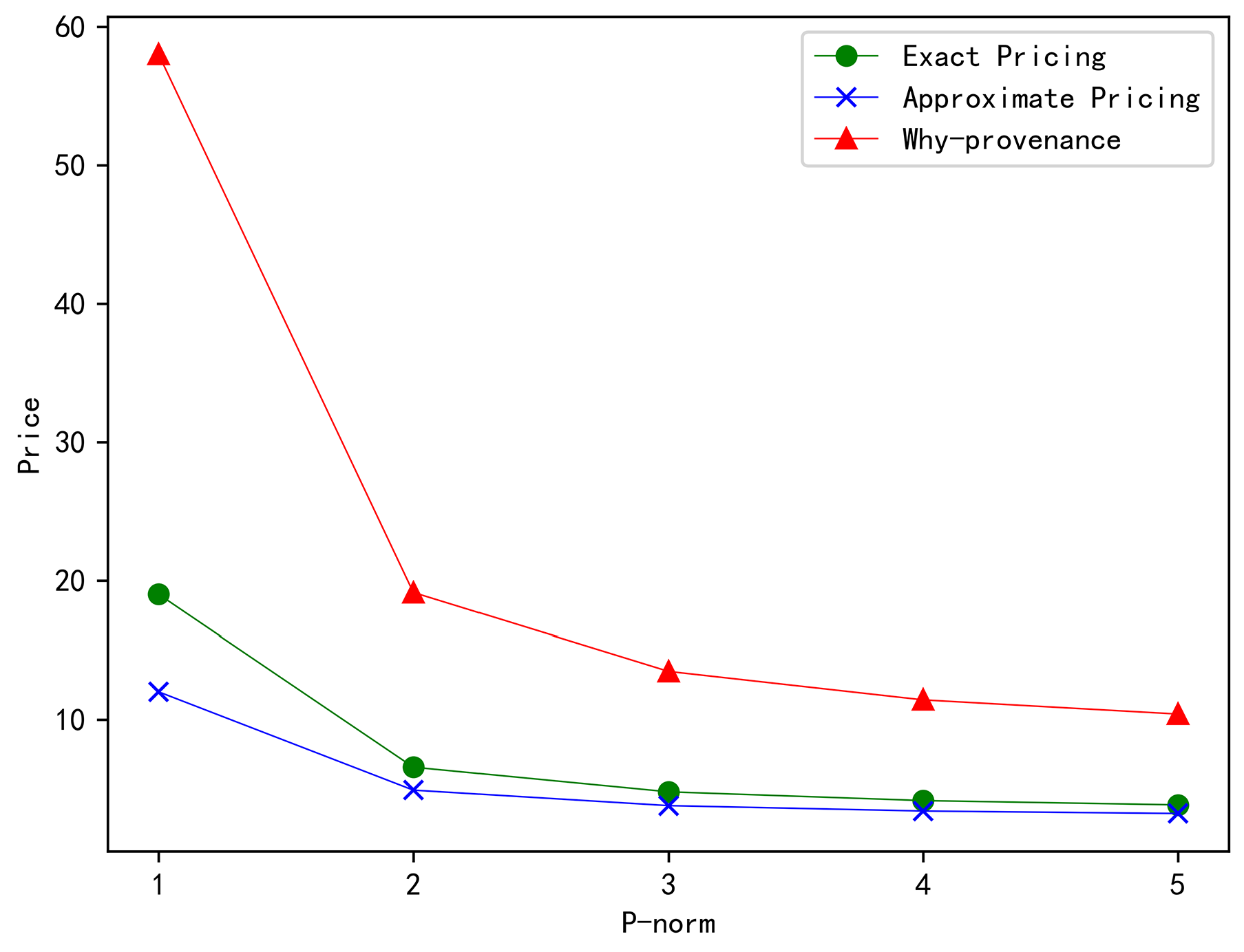
Compared with why-provenance [12], the proposed model used minimal provenance to eliminate unnecessary result tuples in the query result, so our pricing was more accurate and lower. Thus, as depicted in Figure 1, the price of why-provenance was much more expensive than our pricing model. When the p value of the p-norm was used to adjust the price, the higher p was, the lower the price was, and the price was highest when p was one. Similarly, when the p of p-norm was used to adjust the performance ratio, the higher the p was, the lower the performance ratio was, and the highest performance ratio was reached when p was one.

Although Theorem 3 says that calculating the exact price of a query is NP-hard, we show that computing the exact price of the query with selection and join can only be achieved in polynomial time.

Firstly, we performed a selection and join query on the shuhuibao dataset. Let us consider a parameterized query $Q_u^{\bowtie }$:

select$c.User\_ID$, $c.Amount$, $c.Price$as$c\_price$, $m.Price$as$m\_price$from$consume$c, $message$mwhere$c.User\_ID$ = $m.User\_ID$ limit n;

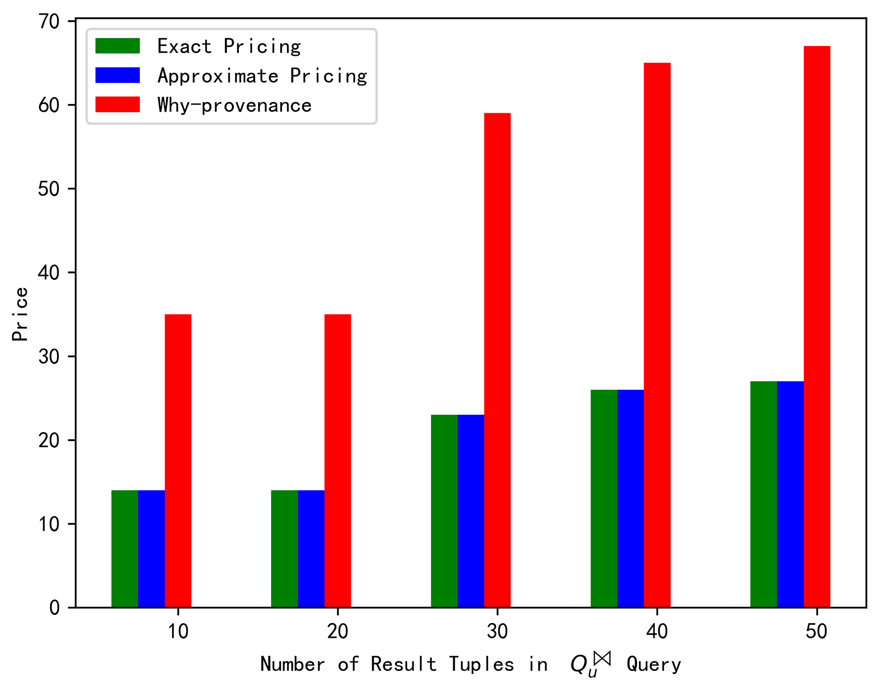
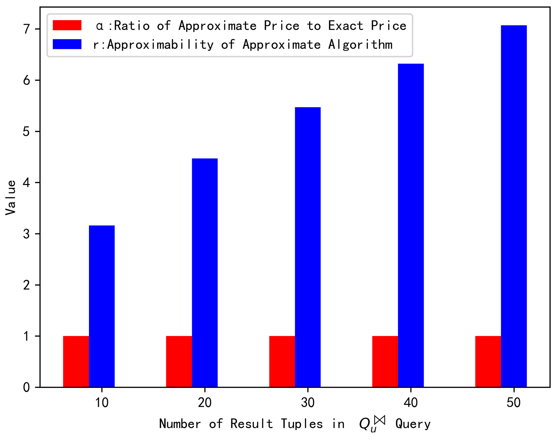
When the number of result tuples n was 10, 20, 30, 40, and 50, the query price of our exact and approximate pricing was 14, 14, 23, 26, and 24, respectively, whereas the why-provenance calculated the query price to be 35, 35, 59, 65, and 67, respectively. It can be intuitively observed from Figure 2 that the exact price is equal to the approximate price, but much less than the why-provenance price, and they maintained a linear increasing relationship with the result tuples, which conformed to the consistency between the number of result tuples and the price, i.e., the more result tuples, the higher the price. The ratio $\alpha$ between the approximate price and the exact price was 1, 1, 1, 1, and 1, respectively. When setting $p=1$ for the p-norm, the performance ratio $r=\sqrt[p]{n}$ value was 3.16, 4.47, 5.47, 6.32, and 7.07, respectively. It can be intuitively observed from Figure 3 that the value of $\alpha$ was far less than the value of r, which further proved that the approximate pricing that we proposed was very effective.

Next, we performed complex queries on the MovieLens dataset. Let us consider a complex query with multiple tables and multiple logics:

select$r.UserID$, $r.MovieID$, $r.Rating$, $r.Price$, $u.User$$ID$, $u.Gender$, $u.Price$from$ratings$r, $users$uwhere$(r.MovieID=1$or$r.MovieID=2)$and$(r.UserID=u.UserID)$limitn;

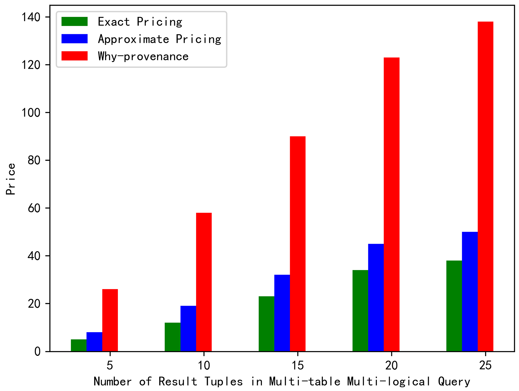
When the number of result tuples n was 5, 10, 15, 20, and 25, the query price of our exact pricing was 5, 12, 23, 34, and 38, the approximate pricing was 8, 19, 32, 45, and 50, and the why-provenance calculated the query price to be 26, 58, 90, 123, and 138, respectively. It can be intuitively observed from Figure 4 that the exact price was slightly lower than the approximate price, but much less than the why-provenance price, and they maintained a linear increasing relationship with the result tuples, which conformed to the consistency between the number of result tuples and the price, i.e., the more result tuples, the higher the price. The ratio $\alpha$ between the approximate price and the exact price was 1.6, 1.58, 1.39, 1.32, and 1.31, respectively. When setting $p=1$ for the p-norm, the performance ratio $r=\sqrt[p]{n}$ value was 2.23, 3.16, 3.87, 4.47, and 5, respectively. It can be intuitively observed from Figure 5 that the value of $\alpha$ was far less than the value of r, which further proves that the approximation algorithm that we proposed was very effective.

5.2. Efficiency

This section studies the efficiency of the algorithm from different dimensions. The running time and memory consumption of the different algorithms were verified by performing different query operations on the two datasets.

Firstly, we still considered the parameterized query that contained selection and join in the previous section $Q_u^{\bowtie }$:

select$c.User\_ID$, $c.Amount$, $c.Price$as$c\_price$, $m.Price$as$m\_price$from$consume$c, $message$mwhere$c.User\_ID$ = $m.User\_ID$ limit n;

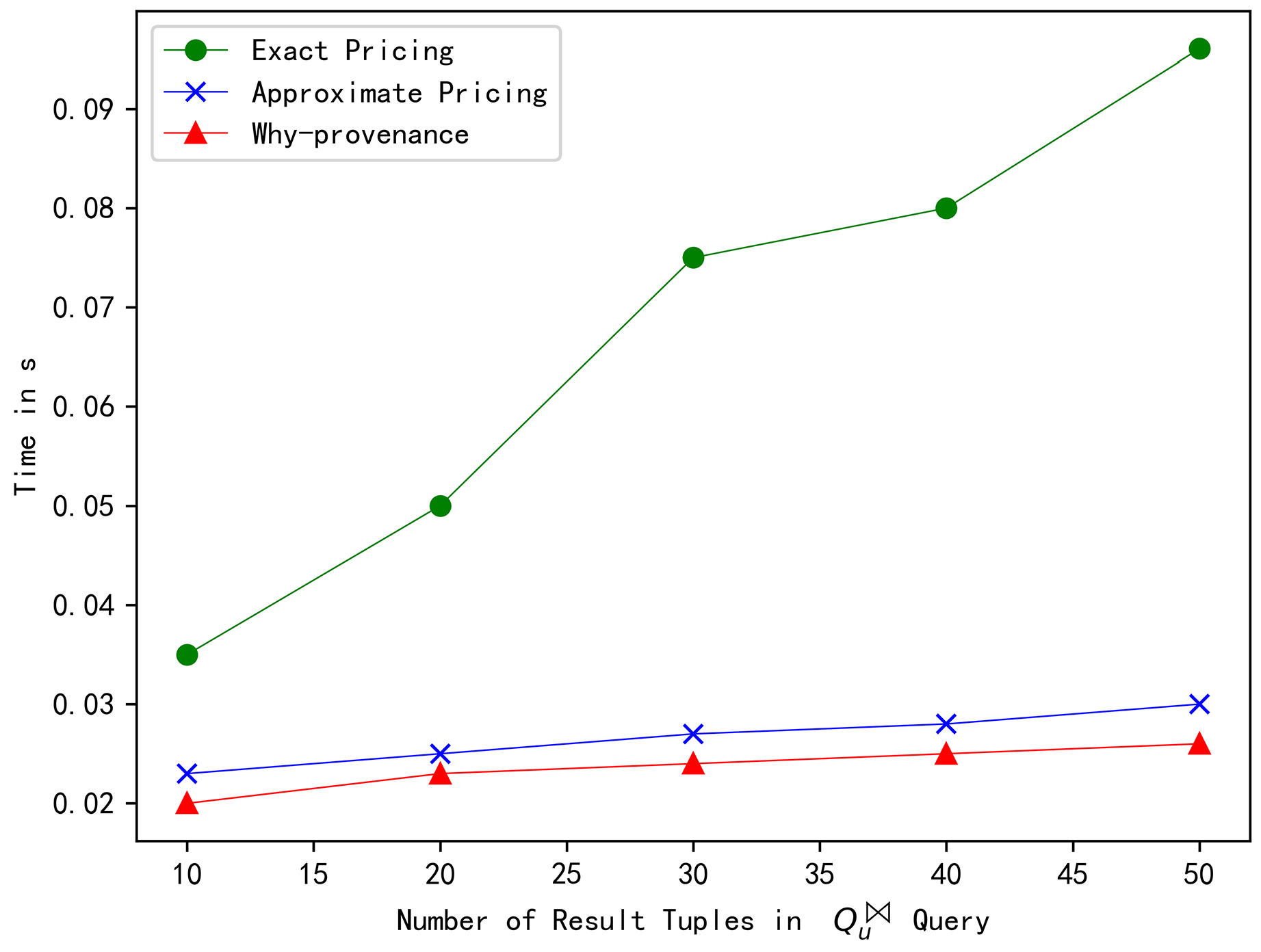
When the number of result tuples n was 10, 20, 30, 40, and 50, the exact pricing calculated the query price in 0.035 s, 0.050 s, 0.075 s, 0.080 s, and 0.096 s, the approximate pricing calculated the query price in 0.023 s, 0.025 s, 0.028 s, 0.028 s, and 0.030 s, and the why-provenance calculated the query price in 0.023 s, 0.025 s, 0.026 s, 0.026 s, and 0.026 s, respectively. It can be observed intuitively from Figure 6 that the run time of the exact pricing was much greater than that of the approximate pricing, but the run time of the approximate pricing was slightly larger than that of the why-provenance, and they maintained a linear increasing relationship with the number of result tuples. The experimental results show that the approximate pricing was more effective. Even for a simple join query, the exact pricing can calculate the query price in polynomial time, but the run time was much longer than the approximate algorithm. Although the run time of approximate pricing was slightly higher than why-provenance, its price was much lower than why-provenance. This result further proved that the approximate pricing was very efficient.

Next, we will still consider a complex query with multiple tables and multiple logics on the MovieLens dataset:

select$r.UserID$, $r.MovieID$, $r.Rating$, $r.Price$, $u.User$$ID$, $u.Gender$, $u.Price$from$ratings$r, $users$uwhere$(r.MovieID=1orr.MovieID=2)$and$(r.UserID=u.UserID)$limitn;

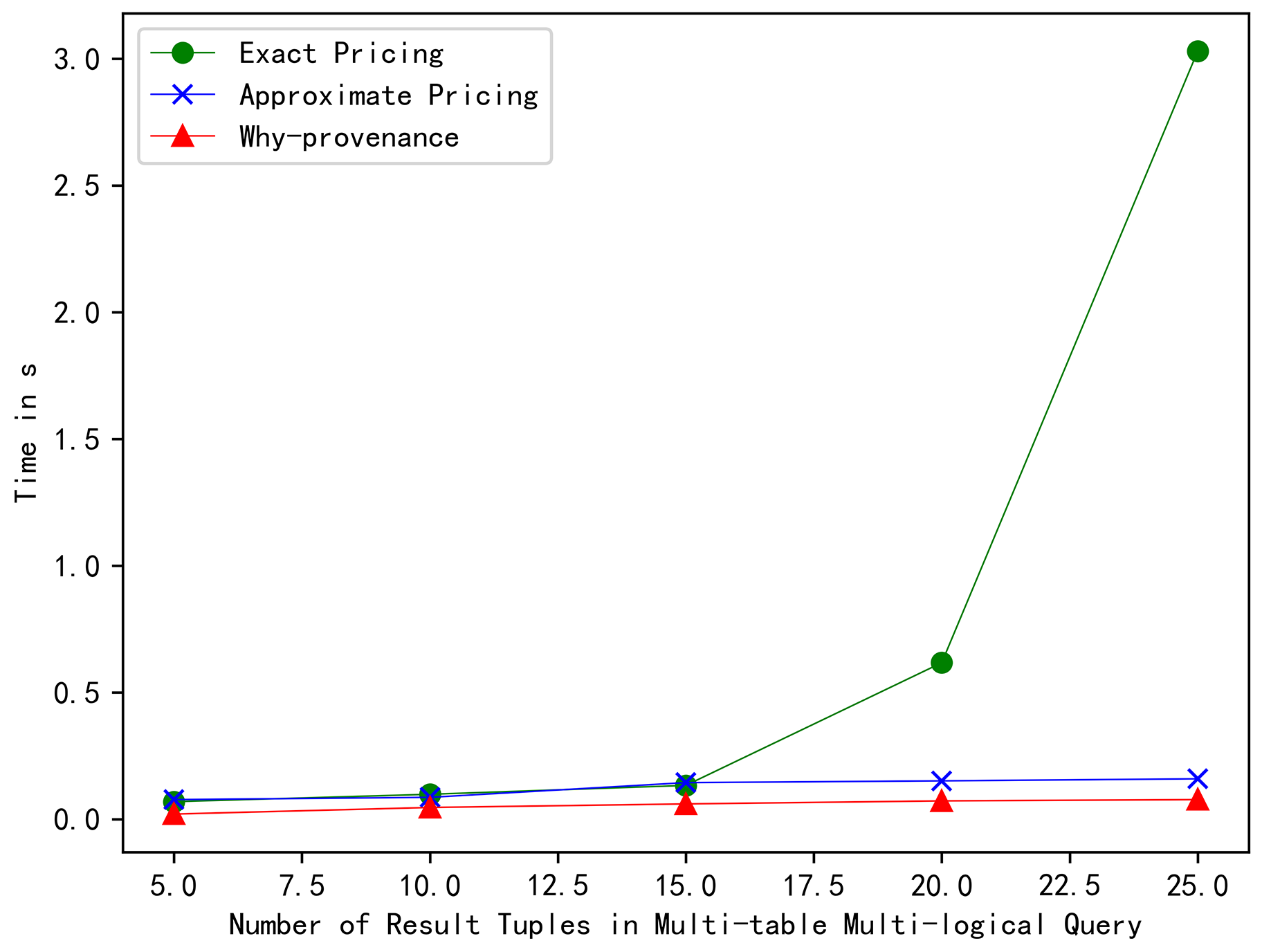
When the number of result tuples n was 5, 10, 15, 20, and 25, the exact pricing calculated the query price in 0.070 s, 0.099 s, 0.134 s, 0.618 s, and 3.03 s, the approximate pricing calculated the query price in 0.078 s, 0.087 s, 0.145 s, 0.152 s, and 0.160 s, and the why-provenance calculated the query price in 0.021 s, 0.047 s, 0.061 s, 0.073 s, and 0.078 s, respectively. It can be observed intuitively from Figure 7 that the run time of the exact pricing was much greater than that of the approximate pricing, but the run time of the approximate pricing was slightly larger than that of the why-provenance, and they maintained a linear increasing relationship with the number of result tuples. The experimental results showed that the approximate pricing was more effective. Even for a simple join query, the exact pricing can calculate the query price in polynomial time. However, for a complex query, the run time of exact pricing would increase exponentially with the increase of the number of result tuples. As can be seen from Figure 7, when the number of result tuples was 25, the run time reached 3 s, which further proved that the time complexity of calculating exact pricing was NP-hard. Although the run time of approximate pricing was slightly higher than why-provenance, its price was much lower than why-provenance. This result further proves that the approximate pricing was very efficient.

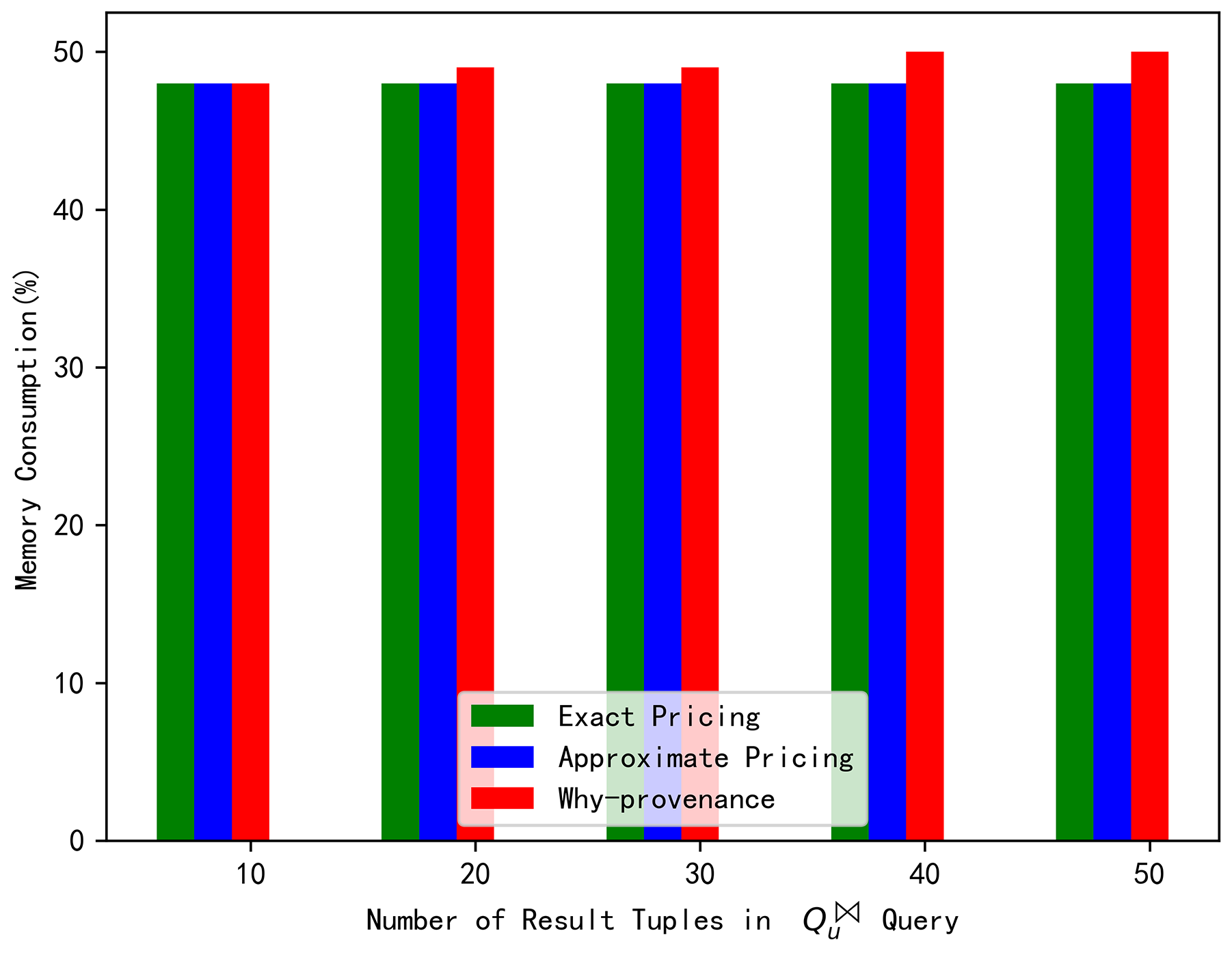
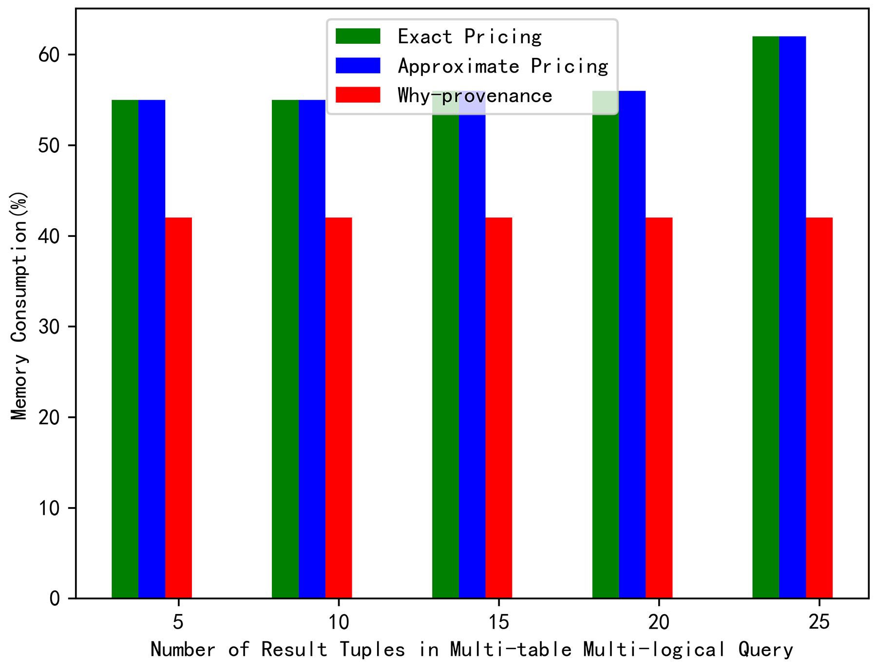
Finally, from Figure 8, we can see that the memory cost of why-provenance was greater than the exact pricing and approximate pricing when performing the join query. However, Figure 9 shows that the memory cost of exact and approximate pricing was greater than why-provenance when complex query was executed. In terms of memory consumption alone, our model might consume more memory. However, our model considered removing redundant and unnecessary result tuples, pursuing minimum provenance, and obtaining the lowest query price. That is the most important thing.

6. Related Work

In the field of pricing mechanism design, there are two crucial focuses of research: query-based pricing and privacy-based pricing.

Query-based pricing: Muschalle et al. [16] observed flat-fee tariffs, usage-based prices, two-part tariffs, package pricing, free pricing, and freemium to be the main pricing strategies. Balazinska et al. [17] believed that the existence of arbitrage opportunities, tuples being able to have the same value, per-query costs being irrelevant, and the lack of a feasible method for data providers to price tiers were four weaknesses of current pricing models. Tang et al. [22] proposed a pricing model that was based on minimal provenance, which is a collection of tuples that contribute to a query. In [23], the concept of data view was proposed; this concept is equivalent to the version of the information product. Koutris et al. [7] proposed a pricing function and proved that it uniquely satisfies the arbitrage-free and discount-free conditions. The least expensive view set determines the price of the query. Deep et al. [24] proposed a framework for arbitrage-free pricing of queries. Lin et al. [25] studied the security implications of query pricing: how to set prices for data queries while protecting the seller’s revenue (preventing arbitrage). Deep et al. [26] presented a scalable pricing framework in which the data provider can choose a variety of pricing functions and control the price of the data by specifying the relation and attribute-level parameters; different parts of the data were assigned different values.

Privacy-based pricing: Niu et al. [21] proposed the first pricing framework ERATOfor the data markets providing common aggregate statistics over private correlated data. In [27], Gkatzelis et al. discussed the privacy attitude, by which individuals were properly compensated and the private data of the data market could be sampled in an unbiased manner by the purchaser. In [28], it was recommended that private data be sold via auction, either completely hidden or completely public. Li et al. [29] studied a balanced privacy data pricing framework in which the purchaser purchases the query data with noise and the data owner is compensated accordingly according to the privacy loss. In [30], Acquisti et al. indicated that privacy valuations are highly dependent on subtle scenarios and are inconsistent. Niu et al. [31] proposed an effective data market security model, which can guarantee data authenticity and protect privacy. Nget et al. [32] considered a practical personal data trading framework that strikes a balance between money and privacy.

Our pricing model was also query-based, but unlike previous work, our pricing model was based on tuple granularity and minimal provenance. In addition, we proposed an exact algorithm and an approximate algorithm to calculate the price of the query, and verified it by instantiation on two real datasets. The original intention of our work is that all source tuples that contributed to the query result were reasonably priced.

7. Conclusions

This paper presented a creative personal data pricing model in accordance with the minimum set of source tuples that contribute to the query results. Our pricing model first set prices for source tuples according to their importance and then performed query pricing based on data provenance, which considered both the importance of the data themselves and the relationships between the data. It was shown that our pricing model was monotonic, bounded, and arbitrage-free. We presented an exact algorithm to calculate the exact price of a query with exponential complexity. Furthermore, we designed an easy approximate algorithm that could calculate the approximate price of the query in polynomial time. In addition, we instantiated our model with the select-joint query and complex query and extensively evaluated its performances on two practical datasets. The experimental results showed that our pricing model was effective and efficient.

References

- Shen, Y.C.; Guo, B.; Shen, Y.; Duan, X.L.; Dong, X.Q.; Zhang, H. A pricing model for Big Personal Data. Tsinghua Sci. Technol. 2016, 21, 482–490. [Google Scholar] [CrossRef]
- Guo, B.; Li, Q.; Duan, X.L.; Shen, Y.C.; Dong, X.Q.; Zhang, H.; Shen, Y.; Zhang, Z.L.; Luo, J. Personal Data Bank: A New Mode of Personal Big Data Asset Management and Value-Added Services Based on Bank Architecture. Chin. J. Comput. 2017, 40, 126–143. [Google Scholar] [CrossRef]
- Durkee, D. Why cloud computing will never be free. Commun. ACM 2010, 53, 62–69. [Google Scholar] [CrossRef]
- Moiso, C.; Minerva, R. Towards a user-centric personal data ecosystem The role of the bank of individuals’ data. In Proceedings of the International Conference on Intelligence in Next Generation Networks, Berlin, Germany, 8–11 October 2012; pp. 202–209. [Google Scholar]
- Chen, R.; Fung, B.C.M.; Mohammed, N.; Desai, B.C.; Wang, K. Privacy-preserving trajectory data publishing by local suppression. Inf. Sci. 2013, 231, 83–97. [Google Scholar] [CrossRef] [Green Version]
- Ng, I.C.L.; Ho, S.Y. Creating New Markets in the Digital Economy: Value and Worth; Cambridge University Press: Cambridge, UK, 2014; pp. 124–125. [Google Scholar]
- Koutris, P.; Upadhyaya, P.; Balazinska, M.; Howe, B.; Dan, S. Query-Based Data Pricing. J. ACM 2015, 62, 1–44. [Google Scholar] [CrossRef]
- Dai, C.; Dan, L.; Bertino, E.; Kantarcioglu, M. An Approach to Evaluate Data Trustworthiness Based on Data Provenance. In Proceedings of the Workshop on Secure Data Management, Auckland, New Zealand, 24 August 2008; pp. 82–98. [Google Scholar]
- Huang, L.; Cheng, H.B. Query Optimization Based on Data Provenance. Adv. Mater. Res. 2011, 186, 586–590. [Google Scholar] [CrossRef]
- Xing, N.; Kapoor, R.; Glavic, B.; Gawlick, D.; Zhen, H.L.; Radhakrishnan, V. Provenance-Aware Query Optimization. In Proceedings of the 2017 IEEE 33rd International Conference on Data Engineering (ICDE), San Diego, CA, USA, 19–22 April 2017; pp. 473–484. [Google Scholar]
- Buneman, P.; Khanna, S.; Wang, C.T. Why and Where: A Characterization of Data Provenance. In Proceedings of the International Conference on Database Theory, London, UK, 4–6 January 2001; pp. 316–330. [Google Scholar]
- Cui, Y.; Widom, J. Practical Lineage Tracing in Data Warehouses. In Proceedings of the 16th International Conference on Data Engineering (Cat. No.00CB37073), San Diego, CA, USA, 29 February–3 March 2000; pp. 367–378. [Google Scholar]
- Green, T.J.; Karvounarakis, G.; Tannen, V. Provenance semirings. In Proceedings of the 26th ACM SIGMOD-SIGACT-SIGART Symposium on Principles of Database Systems, Beijing, China, 11–13 June 2007; pp. 31–40. [Google Scholar]
- Gallone, F. Quantum Mechanics in Hilbert Space; World Scientific Publishing: Singapore, 2015; pp. 611–696. [Google Scholar]
- Cheney, J.; Chiticariu, L.; Tan, W.C. Provenance in Databases: Why, How, and Where. Found. Trends Databases 2007, 1, 379–474. [Google Scholar] [CrossRef]
- Muschalle, A.; Stahl, F.; Löser, A.; Vossen, G. Pricing Approaches for Data Markets. In Proceedings of the 38th International Conference on Very Large Databases, Istanbul, Turkey, 27 August 2012; pp. 129–144. [Google Scholar]
- Balazinska, M.; Howe, B.; Suciu, D. Data Markets in the Cloud: An Opportunity for the Database Community. In Proceedings of the 37th International Conference on Very Large Data Bases, Seattle, Washington, 1 August 2011; pp. 1482–1485. [Google Scholar]
- Xiao, Y.L. Optimization Algorithms for the Minimum-Cost Satisfiability Problem. Ph.D. Thesis, Department of Electrical and Computer Engineering, North Carolina State University, North Carolina, NC, USA, 2004. [Google Scholar]
- Khanna, S.; Trevisan, L.; Williamson, D.P. The Approximability of Constraint Satisfaction Problems. SIAM J. Comput. 2001, 30, 1863–1920. [Google Scholar] [CrossRef] [Green Version]
- MovieLens 1M Dataset. 2003. Available online: https://grouplens.org/datasets/movielens/1m/ (accessed on 16 August 2019).
- Niu, C.Y.; Zheng, Z.Z.; Wu, F.; Tang, S.J.; Gao, X.F.; Chen, G.H. Unlocking the Value of Privacy: Trading Aggregate Statistics over Private Correlated Data. In Proceedings of the 24th ACM SIGKDD International Conference on Knowledge Discovery and Data Mining, London, UK, 19–23 August 2018; pp. 2031–2040. [Google Scholar]
- Tang, R.; Wu, H.; Bao, Z.; Bressan, S.E.; Valduriez, P. The Price is Right: Models and Algorithms for Pricing Data. In Proceedings of the 24th International Conference on Database and Expert Systems Applications, Prague, Czech Republic, 29 August 2013; pp. 380–394. [Google Scholar]
- Balazinska, M.; Howe, B.; Koutris, P.; Dan, S.; Upadhyaya, P. A Discussion on Pricing Relational Data; Springer: Berlin, Germany, 2013; pp. 167–173. [Google Scholar]
- Deep, S.; Koutris, P. The Design of Arbitrage-Free Data Pricing Schemes. In Proceedings of the 20th International Conference on Database Theory, Venice, Italy, 21–24 March 2017; pp. 1–18. [Google Scholar]
- Lin, B.R.; Kifer, D. On arbitrage-free pricing for general data queries. In Proceedings of the 40th International Conference on Very Large Databases, Hangzhou, China, 1–5 September 2014; pp. 757–768. [Google Scholar]
- Deep, S.; Koutris, P. QIRANA: A Framework for Scalable Query Pricing. In Proceedings of the 2017 ACM SIGMOD International Conference on Management of Data, Chicago, IL, USA, 14–19 May 2017; pp. 699–713. [Google Scholar]
- Gkatzelis, V.; Aperjis, C.; Huberman, B.A. Pricing private data. Electron. Mark. 2015, 25, 109–123. [Google Scholar] [CrossRef]
- Riederer, C.; Erramilli, V.; Chaintreau, A.; Krishnamurthy, B.; Rodriguez, P. For sale: Your data: by: You. In Proceedings of the 10th ACM SIGCOMM Workshop on Hot Topics in Networks, Cambridge, MA, USA, 14–15 November 2011; pp. 1–6. [Google Scholar]
- Li, C.; Li, D.Y.; Miklau, G.; Suciu, D. A Theory of Pricing Private Data. Commun. ACM 2017, 60, 79–86. [Google Scholar] [CrossRef]
- Acquisti, A.; John, L.; George, L. What Is Privacy Worth? J. Leg. Stud. 2013, 42, 249–274. [Google Scholar] [CrossRef] [Green Version]
- Niu, C.Y.; Zheng, Z.Z.; Wu, F.; Gao, X.F.; Chen, G.H. Achieving Data Truthfulness and Privacy Preservation in Data Markets. IEEE Trans. Knowl. Data Eng. 2019, 31, 105–119. [Google Scholar] [CrossRef]
- Nget, R.; Cao, Y.; Yoshikawa, M. How to Balance Privacy and Money through Pricing Mechanism in Personal Data Market. In Proceedings of the 2017 SIGIR Workshop On eCommerce, Tokyo, Japan, 7–11 August 2017; pp. 1–10. [Google Scholar]
Figure 1.
Price comparison under the p-norm. As the value of p increases from one to five, the price decreases.
Figure 2.
Price comparison under join query.
Figure 3.
Price ratio vs. approximability of the approximate algorithm.
Figure 4.
Price comparison under complex query.
Figure 5.
Figure 6.
Running time by different algorithms in the select-joint query.
Figure 7.
Running time by different algorithms in complex query.
Figure 8.
Memory consumption by different algorithms in select-joint query.
Figure 9.
Memory consumption by different algorithms in complex query.