Hyper-spectral Recovery of Cerebral and Extra-Cerebral Tissue Properties Using Continuous Wave Near-Infrared Spectroscopic Data

Featured Application

Brain healthmonitoring.

Abstract

Near-infrared spectroscopy (NIRS) is widely used as a non-invasive method to monitor the hemodynamics of biological tissue. A common approach of NIRS relies on continuous wave (CW) methodology, i.e. utilizing intensity-only measurements, and, in general, assumes homogeneity in the optical properties of the biological tissue. However, in monitoring cerebral hemodynamics within humans, this assumption is not valid due to complex layered structure of the head. The NIRS signal that contains information about cerebral blood hemoglobin levels is also contaminated with extra-cerebral tissue hemodynamics, and any recovery method based on such a priori homogenous approximation would lead to erroneous results. In this work, utilization of hyper-spectral intensity only measurements (i.e., CW) at multiple distances are presented and are shown to recover two-layered tissue properties along with the thickness of top layer, using an analytical solution for a two-layered semi-infinite geometry. It is demonstrated that the recovery of tissue oxygenation index (TOI) of both layers can be achieved with an error of 4.4%, with the recovered tissue thickness of 4% error. When the data is measured on a complex tissue such as the human head, it is shown that the semi-infinite recovery model can lead to uncertain results, whereas, when using an appropriate model accounting for the tissue-boundary structure, the tissue oxygenation levels are recovered with an error of 4.2%, and the extra-cerebral tissue thickness with an error of 11.8%. The algorithm is finally used together with human subject data, demonstrating robustness in application and repeatability in the recovered parameters that adhere well to expected published parameters.

1. Introduction

The application of near-infrared spectroscopy (NIRS) is well known in brain health monitoring, and has been used in many clinical settings to monitor cerebral oxygenation during cardiac surgery [1,2]. The most commonly used NIRS instrumentation is a continuous wave (CW) system that is based on the light intensity measurements, i.e., near-infrared light is sent into the tissue and the intensity of the diffusely reflected light is measured. These are of low cost, robust, and have high signal-to-noise ratio, but due to the limited available information of the light propagation, these systems rely on approximations of scattering properties and using simpler homogenous models for parameter recovery. There are other sophisticated systems such as frequency domain (FD) and time domain (TD) NIRS systems, which, additionally to the intensity measurements, can also measure the average time of flight and the distribution of time of flight of photons through the tissue. However, due to the low SNR of TD and FD systems at a relatively high cost, CW systems are widely preferred for cerebral health monitoring.

The parameters of interest are mainly hemoglobin concentration and tissue oxygenation index. Most of the parameter recovery algorithms of CW systems assume a homogenous tissue for the investigated region [3], which is not true for understanding cerebral hemodynamics as the head consists of extra-cerebral tissue between the source-detectors and the cerebral tissue and this can lead to quantification errors. Multi-distance algorithms have been proposed using gradient of intensity attenuation measurements [4,5,6] based on a flat semi-infinite homogenous model. Since the gradient is more sensitive to deeper regions than raw intensity, this makes the recovered parameters less sensitive to changes in extra-cerebral tissue. However, the accuracy of the recovered cerebral tissue parameters still remains low due to the homogenous approximation of the head and due to the curvature and complex internal structure of the head. The assumption of scattering properties of the tissue is another source of error in these gradient-based algorithms. This uncertainty due to scatter approximation has been investigated and an alternative method was proposed [7] to recover scattering parameters and scaled hemoglobin concentrations for a more accurate estimate of tissue oxygenation. Other works that are aimed at the removal of signal contamination due to extra-cerebral layer include: signal regression-based methods [8,9] for recovering changes rather than absolute values. Frequency domain-based methods [10,11] have been proposed that can recover both absorption and scattering properties of extra-cerebral and cerebral tissues along with the thickness of the top layer. In CW-based methods however, phantom studies on a two layered model have been studied with a known superficial layer thickness. [12] The work reported to date has relied on spectral and spatial derivative measurements, where a theoretical non-uniqueness is unavoidable (as detailed in later sections). The unknown superficial layer thickness, and the performance of a two layered model in a realistic scenario with oxy and deoxyhemoglobin as the primary absorption constituents remains unexplored. This is a crucial point to address since the spectral characteristics play a major role in distinguishing the tissue parameters in any recovery algorithm.

With no constraint on the spatial distribution of the optical properties, it has been shown that there can be more than one solutions to CW diffusion equation [13] and with optimal choice of wavelengths this non-uniqueness can be avoided by spectrally constraining the parameter recovery process [14]. In this work, the uniqueness/non-uniqueness problem of a CW system [13] in the context of a layered medium is addressed, by assuming regional homogeneity; it is shown that the solution set is unique if the measured boundary data is intensity-based only. Based on this a two-layered parameter recovery approach is defined for a multi-distance continuous wave hyper-spectral system, to recover the tissue parameters of two layers corresponding to cerebral and extra-cerebral regions as well as the superficial tissue thickness. The study is divided into three parts, the first part deals with data simulated and parameter recovery using the two-layered semi-infinite model, second part deals with data simulated on two-layered head model but the parameter recovery is implemented using two-layered semi-infinite model, third part deals with data simulated on two-layered head model and parameter recovery is also based on a head model. The proposed method is then implemented and used to recover the cerebral and extra-cerebral tissue parameters of a human subject by measuring NIRS data on the forehead to demonstrate the practical viability of the approach.

2. Continuous Wave Data and Uniqueness in Parameter Recovery

Uniqueness/non-uniqueness problem in the parameter recovery methods of CW-based systems has been a long-discussed topic [13,14] and has been shown that for a single wavelength multi-distance boundary intensity measurements there can be more than one solutions of absorption and reduced scattering coefficient distributions which will lead to the same boundary data. This non-uniqueness can be addressed by using multi-wavelength data and constraining the problem spectrally [14]. The reported findings to date discuss a very general scenario of image reconstruction where the recovered parameters are the three-dimensional distribution of absorption and reduced scattering coefficients. However, in the context of finding the absolute parameters of different regions in a layered medium such as the human head, this presented work brings an additional spatial constraint to the distribution of parameters. Here, by extending the arguments made in previous works [13,14] it is shown that given such a regional constraint on parameters, each solution set is unique to a measured boundary intensity data, and also investigates the scenario when the measured data is either a spatial or 1^st spectral derivative of intensity (in log scale).

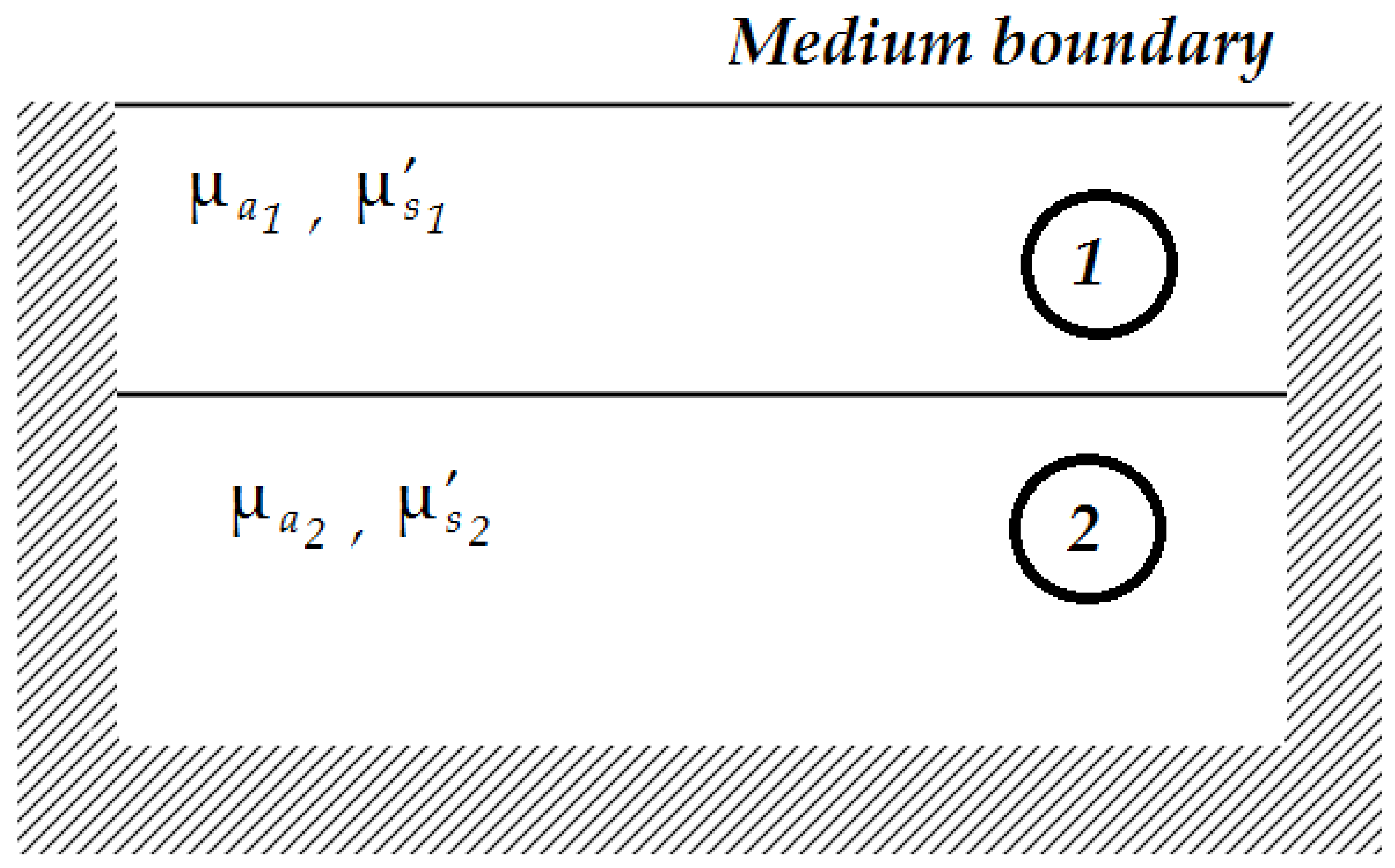
Consider the following schematic of a two-layered medium as shown in Figure 1.

Here, ${\mu }_a$ is the absorption coefficient, ${\mu }_s^{\prime }$ is the reduced scattering coefficient, and the diffusion coefficient ($D$) is defined as, $D=1/3\left({\mu }_a+{\mu }_s^{\text{'}}\right)\approx 1/3{\mu }_s^{\text{'}}$. Re-writing the CW diffusion equation by change of variables to get the Helmholtz-type equation given as [13],

$$-{\nabla }^2\mathsf{\Psi }+\eta \mathsf{\Psi }=\frac{q_0}{\gamma }.$$

(1)

where ${\gamma }^2=D$, $q_0$ is the source distribution, $\mathsf{\Psi }=\gamma \mathsf{\Phi }$, where $\mathsf{\Phi }$ is the photon density, and the variable $\eta$ is given by,

$$\eta =\frac{{\nabla }^2\gamma }{\gamma }+\frac{{\mu }_a}{{\gamma }^2}.$$

(2)

Considering the light-source to be a point source at a location $r_0$ on the external medium boundary, and defining ${\mathsf{\Psi }}_0$ such that:

$$-{\nabla }^2{\mathsf{\Psi }}_0+\eta {\mathsf{\Psi }}_0={\mathrm{q}}_0.$$

(3)

This implies that $\mathsf{\Psi }={\mathsf{\Psi }}_0/\gamma \left(r_0\right)={\mathsf{\Psi }}_0/{\gamma }_1$, as $\gamma \left(r_0\right)={\gamma }_{boundary}={\gamma }_1$ in the given scenario and therefore ${\mathsf{\Phi }}_{\mathrm{boundary}}={\mathsf{\Psi }}_0{}_{boundary}/{\gamma }_1^2$.

For any measured boundary intensity data ${\mathsf{\Phi }}_{\mathrm{boundary}}$, two non-unique solution sets $\left\{{\mu }_a, {\mu }_s^{\text{'}},L\right\}$ and $\left\{{\tilde{\mu }}_a, {\tilde{\mu }}_s^{\text{'}}, \tilde{L}\right\}$ (with their equivalent canonical parameters $\eta$ and $\tilde{\eta }$), can exist if they satisfy the following two conditions:

Condition-1: $\eta =\tilde{\eta }$ everywhere inside the medium, this ensures ${\mathsf{\Psi }}_0$ to be the same for both solutions.

Condition-2: ${\gamma }_{boundary}={\tilde{\gamma }}_{boundary}$, together with condition 1 this ensures ${\mathsf{\Phi }}_{\mathrm{boundary}}$ to be the same for both solutions.

Applying condition 1, to this scenario, $\eta =\tilde{\eta }$ for region-1, region-2 and at the boundary between them. This requires the superficial layer thickness to be equal i.e., $L=\tilde{L}$, as without this the two solutions would have a different location of the interface between region-1 and region-2, and $\eta$ can never be equal to $\tilde{\eta }$ at the regional interface. Solving condition-1 inside region-1 and region-2 (i.e., ${\eta }_1={\tilde{\eta }}_1$ and ${\eta }_2={\tilde{\eta }}_2$ with ${\nabla }^2\gamma =0$), we have:

$${\mu }_{a_1}\cdot {\mu }_{s_1}^{\text{'}}={\tilde{\mu }}_{a_1}\cdot {\tilde{\mu }}_{s_1}^{\text{'}},$$

(4)

$${\mu }_{a_2}\cdot {\mu }_{s_2}^{\text{'}}={\tilde{\mu }}_{a_2}\cdot {\tilde{\mu }}_{s_2}^{\text{'}}.$$

(5)

At the boundary between region-1 and 2, knowing that ${\nabla }^2\gamma \propto \left({\gamma }_2-{\gamma }_1\right)$, and from Equations (4) and (5):

$$\frac{{\gamma }_1}{{\gamma }_2}=\frac{{\tilde{\gamma }}_1}{{\tilde{\gamma }}_2}\Rightarrow \frac{{\mu }_{s_1}^{\text{'}}}{{\mu }_{s_2}^{\text{'}}}=\frac{{\tilde{\mu }}_{s_1}^{\text{'}}}{{\tilde{\mu }}_{s_2}^{\text{'}}}$$

(6)

Similar analysis can be extended for more than two regions if needed and therefore the solution set $\left\{{\tilde{\mu }}_a, {\tilde{\mu }}_s^{\text{'}}\right\}$ should be of the form $\left\{\alpha {\mu }_a, {\alpha }^{-1} {\mu }_s^{\text{'}}\right\}$ everywhere in the medium, for an arbitrary constant$\mathsf{\alpha }$. An equivalent representation of this non-uniqueness expression in terms of spectral parameters chromophore concentrations ($C_{\mathrm{i}}$), scattering amplitude ($Sa$) and scattering power ($Sp$) can be shown as $\left\{{\tilde{C}}_{\mathrm{i}},\widetilde{Sa},\widetilde{Sp}\right\}=\left\{\alpha C_{\mathrm{i}},{\mathsf{\alpha }}^{-1}Sa,\mathrm{Sp}\right\}$, where these spectral parameters are related to the optical properties as follows:

$${\mu }_a\left(\lambda \right)={{\displaystyle \sum }}_{\mathrm{i}=1}^N{\epsilon }_{\mathrm{i}}\left(\lambda \right)\cdot C_{\mathrm{i}}$$

(7)

$${\mu }_s^{\text{'}}\left(\lambda \right)=Sa \cdot {\lambda }^{-Sp}$$

(8)

Here, $C_{\mathrm{i}}$ denotes the concentration of the major chromophores contributing to light absorption, ${\epsilon }_{\mathrm{i}}$ denotes the extinction coefficient of the corresponding chromophore.

Applying condition 2, ${\tilde{\gamma }}_{boundary}={\gamma }_{boundary} \Rightarrow {\tilde{\gamma }}_1={\gamma }_1 \Rightarrow {\tilde{\mu }}_{s_1}^{\text{'}}={\mu }_{s_1}^{\text{'}}$, this gives the value of the arbitrary constant to be $\alpha =1$. This shows that for measured boundary intensity, the solution set is unique with the assumed regional homogeneity.

However, if the measured data is either a spatial or spectral derivative of the form $\log \left({\mathsf{\Phi }}_{\mathrm{boundary}}\left(r_1,{\lambda }_1\right)/{\mathsf{\Phi }}_{\mathrm{boundary}}\left(r_2,{\lambda }_2\right)\right)=\log \left({\mathsf{\Psi }}_0\left(r_1,{\lambda }_1\right)\cdot {\gamma }_1\left({\lambda }_2\right)/{\mathsf{\Psi }}_0\left(r_2,{\lambda }_2\right)\cdot {\gamma }_1\left({\lambda }_1\right)\right)$, any arbitrary value of the constant $\alpha$ leads to the same measured data, thus allowing for a non-unique solution set. In such a scenario, this non-uniqueness leads to uncertain parameter recovery, and this is seen in terms of the cross-talk between chromophore concentrations and scattering amplitude. However, biomarkers such as tissue oxygenation index (TOI), which are based on the ratio of chromophore concentrations, will still be accurate, as all the chromophore concentrations in any of the non-unique solution sets differ only by a common constant factor from true values.

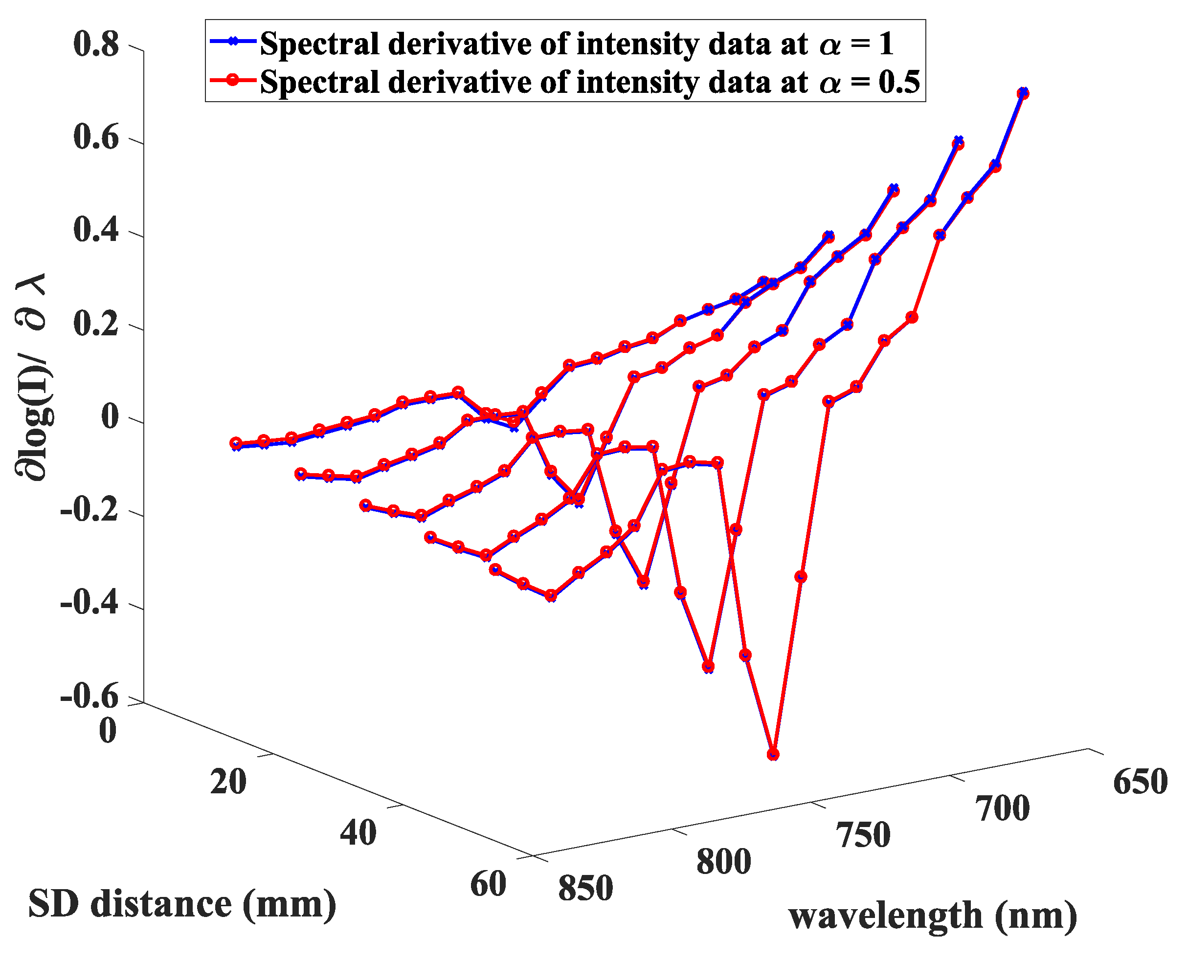
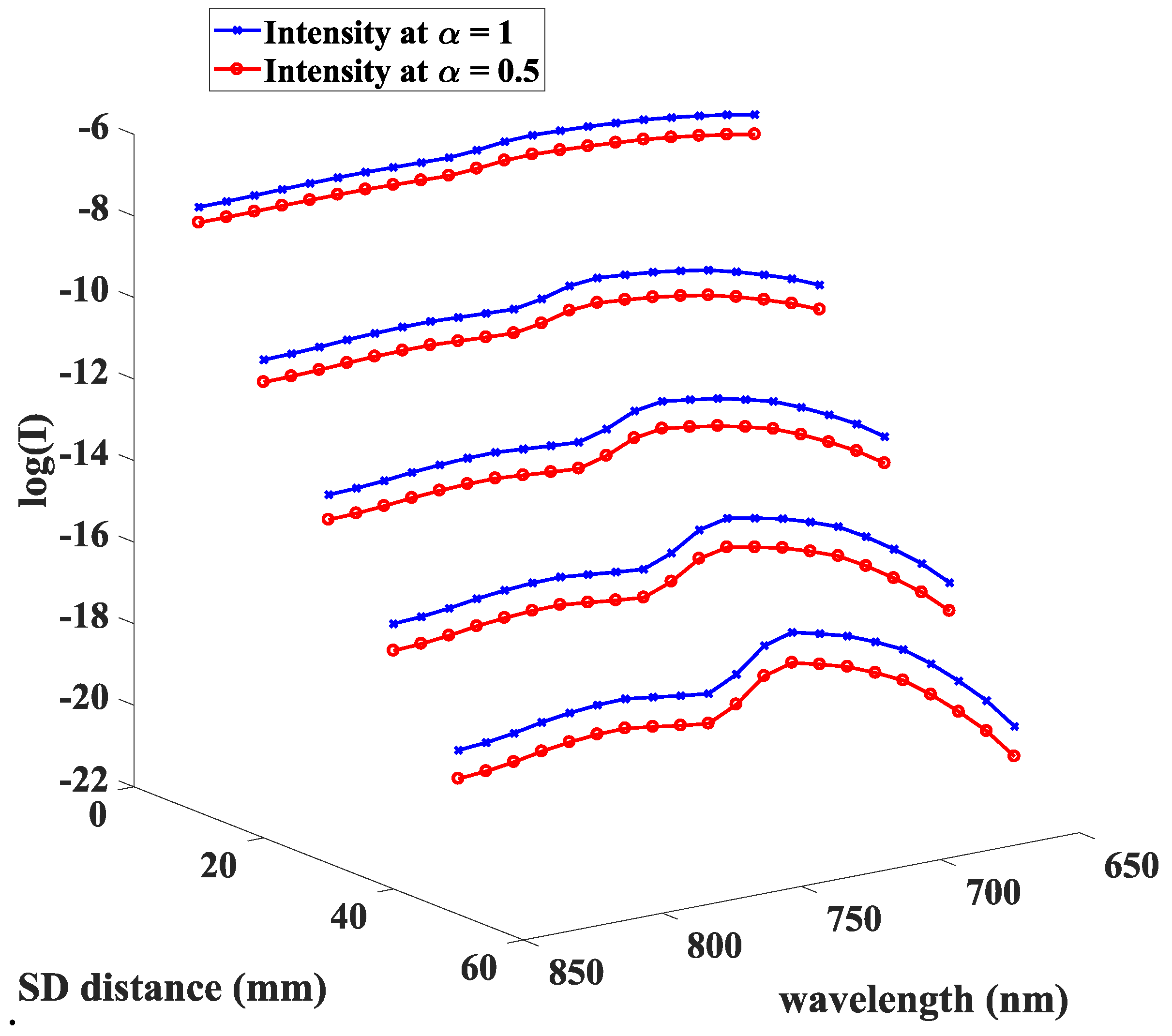
To demonstrate the non-uniqueness in terms of the widely used spectral derivative of intensity data, let us consider an example of a two-layered medium with two major light-absorbing chromophores i.e., oxy-hemoglobin (its concentration denoted by HbO) and deoxy-hemoglobin (its concentration denoted by Hb) with their layer-specific values given as ${\mathrm{HbO}}_1=0.047 \mathrm{mM}$, ${\mathrm{HbO}}_2=0.054 \mathrm{mM}$, ${\mathrm{Hb}}_1=0.011 \mathrm{mM}$, ${\mathrm{Hb}}_2=0.022 \mathrm{mM}$, ${\mathrm{Sa}}_1=0.64{\mathrm{mm}}^{-1}$, ${\mathrm{Sa}}_2=0.98 {\mathrm{mm}}^{-1}$, ${\mathrm{Sp}}_1=1.06$, ${\mathrm{Sp}}_2=0.611$, corresponding to layer-1 and layer-2 respectively, and L=10mm. For the source-detector distances of $\rho =10, 20, 30, 40, 50 \mathrm{mm}$, and wavelengths $\lambda =650 \mathrm{to} 850 \mathrm{nm}$, in steps of 10 nm, the boundary intensity is simulated using NIRFAST [15], which is an open-source finite-element-based model for simulation of light propagation in biological tissue. Figure 2 shows the spectral derivative of intensity data for two distinct parameter sets corresponding to $\alpha =1 \mathrm{and} 0.5$, which are clearly coinciding with each other and their corresponding intensity data is shown in Figure 3.

As evident in Figure 2 and Figure 3, while the intensity data remains distinct for two different ground-truth parameters, the derivative data shows very little variation and therefore demonstrates the non-uniqueness of derivative of intensity data. Hence, in this work, only the intensity data is considered as the measurement for the recovery of absolute tissue parameters. Although uniqueness in terms of intensity data is established from above, one should remember that in a practical scenario, finite independent measurements, noise in the measured data, any mismatch in the assumed model, or the stopping criterion of an iterative fitting method algorithm, can lead to potential recovery errors.

3. Methodology

Initially, the complex structure of the head is simplified into two layers to better understand and distinguish the hemodynamics of cerebral and extra-cerebral (skin and skull) tissues. For a two-layered semi-infinite medium (as shown in Figure 1), the measured boundary intensity at a detector at a distance $\rho$ from a point-source can be written as [16,17]:

$$I\left(\rho \right)=\frac{1}{2\pi }{{\displaystyle \int }}_0^{\infty }\varphi \left(s\right)s J_0\left(s\rho \right)ds,$$

(9)

where, $s$ is the radial spatial frequency coordinate corresponding to the radial distance $\rho$, $J_0$ is the zeroth order Bessel function of first kind, and $\varphi$ is given by:

$$\varphi \left(s\right)=\frac{\sinh \left({\alpha }_1\left(z_b+z_0\right)\right)}{D_1{\alpha }_1}\times \frac{D_1{\alpha }_1\cosh \left({\alpha }_{1}L\right)+D_2{\alpha }_2\sinh \left({\alpha }_{1}L\right)}{D_1{\alpha }_1\cosh \left({\alpha }_1\left(L+z_b\right)\right)+D_2{\alpha }_2\sinh \left({\alpha }_1\left(L+z_b\right)\right)}-\frac{\sinh \left({\alpha }_1{z}_0\right)}{D_1{\alpha }_1}$$

(10)

Here, L is the thickness of layer-1, the subscripts 1 and 2 indicate the properties for layer-1 and layer-2, ${\alpha }_i=\sqrt{s^2+\frac{{\mu }_{a_i}}{D_i}}$, diffusion coefficient $D_i=\frac{1}{3\left({\mu }_{a_i}+{{\mu }^{\prime }}_{s_i}\right)}$, $z_0=\frac{1}{{\mu }_{a_1}+{{\mu }^{\prime }}_{s_1}}$, $z_b=\frac{1+R_{\mathrm{eff}}}{1-R_{\mathrm{eff}}}2D_1$. $R_{\mathrm{eff}}$ is the fraction of photons internally and diffusively reflected at the boundary.

As shown in Section 2, for the measured CW intensity data on the boundary of a two-layered medium a unique solution exists for a parameter set $\left\{{\mu }_{a_1},{\mu }_{{\mathrm{s}}_1}^{\prime },{\mu }_{a_2},{\mu }_{{\mathrm{s}}_2}^{\prime },\mathrm{L}\right\}$. To increase the number of independent measurements and therefore improve the recovery accuracy the problem is spectrally constrained by measuring the intensity data over a broad range of wavelengths. For biological tissues, since hemoglobin is the major absorbing chromophore in the near-infrared range, the wavelength range 650 to 850 nm at either side of the isosbestic region are considered (which is typically conventional in most systems, well away from 950 nm beyond which other molecules, such as Methemoglobin and water are the dominant absorbing chromophores). Although other chromophores have significant extinction coefficients in this wavelength range, their concentration in the tissue is relatively low, therefore oxy and deoxyhemoglobin can be considered as the main absorbers. The parameter set now becomes $p\equiv \left\{Hb{O}_1,Hb{O}_2,H{b}_1,H{b}_2,S{a}_1,S{a}_2,S{p}_1, S{p}_2,L\right\}$, and measurement data is the light intensity at source-detector distances $\rho =10, 20, 30, 40, 50 \mathrm{mm}$, and wavelengths $\lambda =650 \mathrm{to} 850 \mathrm{nm}$, in steps of 10 nm. Instead of a conventional approach of recovering all parameters together using a least-square minimization method which generally exhibits a very high condition number, the recovery of parameters is achieved in two steps: (1) recovering layer-1 parameters from spectral intensity data at $\rho =10 \mathrm{mm}$ i.e., a short source-detector distance, assuming a homogenous model as implemented by considering same parameters of layer-1 and layer-2 properties in Equation (10), the dependency on L is assumed to be minimal in such a case, and (2) utilizing the recovered layer-1 parameters in step-1, the layer-2 parameters and tissue thickness L, are recovered using spectral intensity data from $\rho =10 \mathrm{to} 50 \mathrm{mm}$. This splitting of the parameter recovery is observed to greatly improve the inverse problem with decreasing the condition number by at least an order of magnitude (i.e., by a factor of 10).

Consider the column vectors $p_1\equiv \left\{Hb{O}_1,H{b}_1,S{a}_1,S{p}_1\right\}$, and $p_2\equiv \left\{Hb{O}_2,H{b}_2,S{a}_2,S{p}_2,L\right\}$, denoting the parameter sets for the two step parameter recovery with the corresponding measurement data given by the column vectors $y_1\equiv I\left(\rho , \lambda \right)$ at $\rho =10$ mm and $\lambda =650 \mathrm{to} 850$ nm in steps of 10 nm, and $y_2\equiv I\left(\rho , \lambda \right)$ at $\rho =10 \mathrm{to} 50$ mm in steps of 10 mm, and $\lambda =650 \mathrm{to} 850$ nm in steps of 10 nm. Let ${\mathrm{v}}_m$ be the m-th entry in the column vector $v$, then the element ${\mathrm{j}}_1{}_{mn}$ (of m-th row and n-th column) of the Jacobian (or sensitivity) matrix $J_1$ corresponding to recovery step-1 is given by,

$${\mathrm{j}}_1{}_{mn}=\raisebox{1ex}{$\partial {\mathrm{y}}_1{}_m$}\!\left/ \!\raisebox{-1ex}{$\partial {\mathrm{p}}_1{}_n$}\right..$$

(11)

Similarly, the element ${\mathrm{j}}_2{}_{mn}$ of the Jacobian matrix $J_2$ corresponding to recovery step-2 is given by,

$${\mathrm{j}}_2{}_{mn}=\raisebox{1ex}{$\partial {\mathrm{y}}_2{}_m$}\!\left/ \!\raisebox{-1ex}{$\partial {\mathrm{p}}_2{}_n$}\right..$$

(12)

The inverse problem at each step is then implemented by an iterative regularized least-square minimization, where the data is modelled corresponding to the estimated parameter set at each iteration (beginning with assumed initial values). Based on the mismatch between modelled and measured data the following parameter update equation is calculated at the end of each iteration, [18]

$$\mathsf{\Delta }{p}_i={\left(J_i{}^{\mathrm{T}}{J}_i+\beta I\right)}^{-1} J_i{}^{\mathrm{T}}\mathsf{\Delta }{y}_i.$$

(13)

Here, ‘i’ denotes the recovery step-1 or 2, $\mathsf{\Delta }{p}_i$ represents the update for the parameter set $p_i$, $\mathsf{\Delta }{y}_i$ is the data-model misfit at the end of iteration, and $J_i$ is the corresponding Jacobian matrix. To further aid the stability, the inverse problem is guided with a regularization parameter given by $\beta$, which is considered as 0.01 times the maximum value of the Hessian $J_i{}^{\mathrm{T}}{J}_i$. A relative change of less than 2% in the error corresponding to data-model misfit over two successive iterations is considered as the stopping criteria for the inverse problem.

The simulation study is split into three parts. Part-(1) deals with data generated on a two-layered semi-infinite model and recovered using a two-layered semi-infinite model as well. To consider a more practical scenario, in part-(2) the data is generated on a two-layered head model but parameter recovery is implemented using two-layered semi-infinite model. Part-(3) deals with data generated on head model and recovered using a head model as well. Part-(2) and (3) are compared to see if the semi-infinite model-based recovery is close enough to head-model-based recovery.

4. Results

4.1. Two-layered Semi-infinite Model

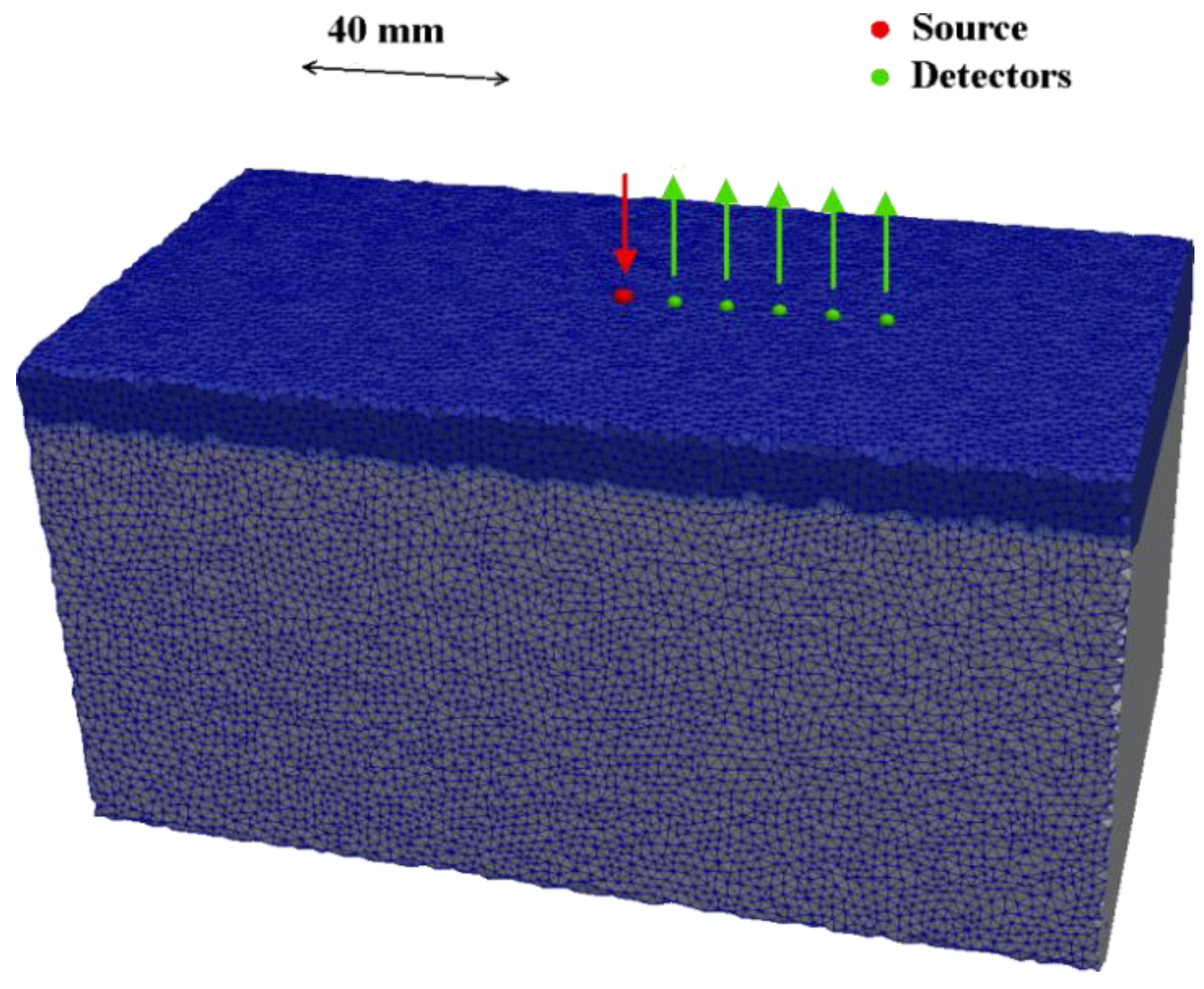
The two-layered semi-infinite model as described in Equations (9) and (10), is employed to simulate the measurement data. The modelled measurement system consists of source-detector distances of 10 to 50 mm in steps of 10 mm, Figure 4, and wavelengths from 650 to 850 nm in steps of 10 nm, and a Gaussian random noise of 1% is added to the data. From previous studies, a noise level from 0.12 to 1.42% is generally added for source-detector separations varying from 13 to 48mm [19], to represent a physical model. In this work, apart from multi-distance measurements varying from 10 to 50 mm, we have broadband wavelength data ranging from 650 to 850 nm, and therefore the distribution of noise levels is more complex than that. Therefore, an average of 1% random noise is applied for all source-detector separations and wavelengths. The tissue properties of the two layers are as shown in

Table 1. Tissue parameters.

	HbT (mM)	TOI (%)	Sa (mm-1)	Sp
Layer-1	0.059	80	0.64 ± 10%	1.0685 ± 10%
Layer-2	0.076	50-80	0.98 ± 10%	0.611 ± 10%

[19,20], and 10 different cases of randomly varying scattering properties (i.e., both Sa and Sp) of both layers are considered with a standard deviation of 10% around the reference values, to include the inter-subject variability in scattering properties. To understand the response of the recovery method to different cerebral oxygenation levels, the TOI of layer-2 was also varied from 50% to 80% which are considered the practical extreme values [21,22]. The sensitivity matrices corresponding to step-1 and step-2 of the recovery process as given in Equations (11) and (12), are calculated using perturbation method on the analytic expression of Equations (9) and (10). The whole simulation study is repeated for different layer-1 thickness values of L = 8, 10, 12 mm which are in the range of practical values for the extra-cerebral thickness of human head.

The recovered TOI values of the two-layers for different thicknesses of layer-1 (8, 10, 12 mm) are as shown in Figure 5 in comparison to the homogenous parameter recovery. The homogenous parameter recovery is similar to step-1 in the proposed two-layered recovery process, but all the measured source-detector distances are considered. The retrieved values of layer-1 thickness is as shown in Figure 6.

The above results (

Table 2. Average percentage error (%) in homogenous and two-layered parameter recovery for different ground-truth scattering parameters and different TOI values of layer-2.

Layer-1 Thickness →		8 mm	10 mm	12 mm
%Δ HbO	Homogenous	−31.5 ± 17.3	−23.8 ± 18.4	−17.8 ± 19.1
	Layer-1	10.0 ± 4.5	8.2 ± 2.6	7.1 ± 1.4
	Layer-2	−16.6 ± 7.2	−15.0 ± 6.1	−15.9 ± 4.9
%Δ Hb	Homogenous	6.1 ± 23.2	16.3 ± 23.3	23.6 ± 22.7
	Layer-1	−15.9 ± 2.6	−13.8 ± 1.9	−13.0 ± 1.2
	Layer-2	−0.3 ± 9.7	0.8 ± 5.2	2.4 ± 3.4
Δ TOI	Homogenous	8.3 ± 8.3	9.5 ± 9.3	10.4 ± 9.9
	Layer-1	−4.4 ± 0.5	−3.6 ± 0.2	−3.3 ± 0.1
	Layer-2	3.2 ± 1.4	3.1 ± 0.9	3.4 ± 0.5
%Δ Sa	Homogenous	39.4 ± 0.6	38.8 ± 0.3	37.8 ± 0.2
	Layer-1	−8.2 ± 2.9	−8.2 ± 1.8	−8.1 ± 0.9
	Layer-2	7.9 ± 4.8	7.6 ± 1.6	6.4 ± 1.1
%Δ Sp	Homogenous	−13.7 ± 0.3	−15.7 ± 0.4	−17.5 ± 0.5
	Layer-1	25.8 ± 0.4	26.1 ± 0.2	26.3 ± 0.1
	Layer-2	−44.9 ± 9.8	−48.8 ± 9.9	−52.4 ± 8.7
%Δ L	Layer-1	3.4 ± 4.4	3.4 ± 4.1	4.0 ± 3.1

) show that the proposed two-layered hyper-spectral parameter recovery method retrieves the tissue oxygenation index and tissue thickness within 4.4% and 4% error respectively. Recovery of other tissue parameters (hemoglobin concentrations and scattering amplitude of two layers) can be obtained within 16.6% error with this two-layered approach, as compared to 31.5% error with the homogenous parameter recovery. However, the scattering power parameter exhibits relatively higher recovery errors due to its low sensitivity to light-intensity.

4.2. Two-layered Head Model

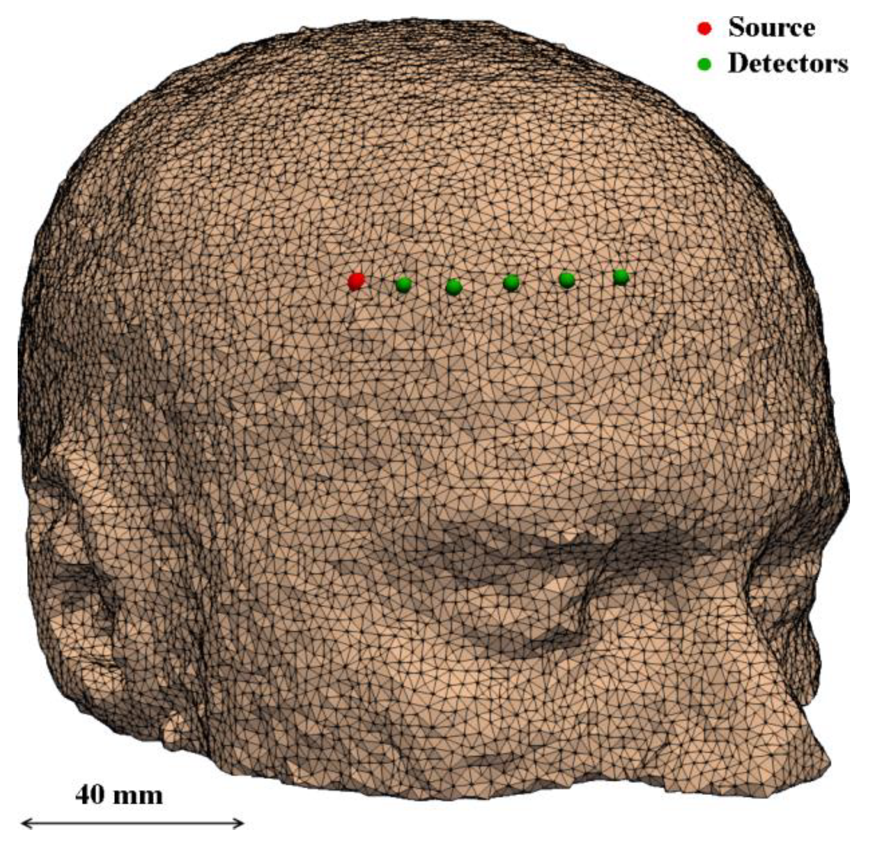
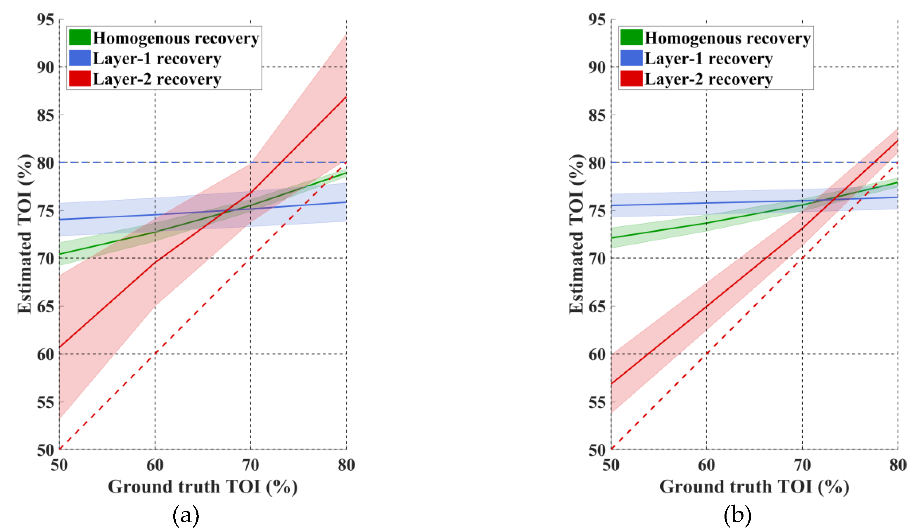
In a realistic scenario, the structure of the head is more complex than a two-layered semi-infinite geometry. Therefore, data were simulated using the same tissue properties as shown in Table 1 on two-layered (cerebral and extra-cerebral tissues) head models using NIRFAST corresponding 10 different subject head models, Figure 7, with their scattering parameters (both Sa and Sp) randomly varying with 10% standard deviation from the reference values shown in Table 1 and the cerebral TOI varying from 50% to 80%, and subsequently the two-step parameter recovery algorithm was utilized, initially, using a two-layered semi-infinite model for the recovery. This was to consider the case where data is from a human subject, but the model utilized for parameter recovery is based on a simple two-layered model. The parameter recovery results are shown in Figure 8a, Figure 9, and

Table 3. Average percentage error (%) in the homogenous and two-layered recovery of parameters corresponding to a semi-infinite recovery model and a head-based recovery model.

Recovery model →		Semi-infinite Recovery Model	Head-based Recovery Model
%Δ HbO	Homogenous	22.0 ± 13..3	−27.2 ± 18.4
	Layer-1	21.9 ± 2.9	5.2 ± 4.4
	Layer-2	19.0 ± 7.5	−23.3 ± 7.6
%Δ Hb	Homogenous	48.3 ± 9.3	15.3 ± 22.5
	Layer-1	−5.5 ± 1.2	−20.0 ± 3.7
	Layer-2	45.4 ± 6.1	−1.36 ± 7.6
Δ TOI	Homogenous	9.3 ± 8.0	9.8 ± 9.0
	Layer-1	−5.1 ± 0.6	−4.1 ± 0.3
	Layer-2	8.4 ± 2.6	4.2 ± 1.9
%Δ Sa	Homogenous	12.3 ± 2.2	37.8 ± 0.4
	Layer-1	−34.0 ± 2.2	−6.2 ± 2.7
	Layer-2	4.4 ± 14.4	16.2 ± 2.7
%Δ Sp	Homogenous	−41.2 ± 4.0	−22.1 ± 0.4
	Layer-1	17.8 ± 0.8	26.8 ± 1.1
	Layer-2	−87.8 ± 58.3	−44.2 ± 7.6

. As some measurement data did not converge to a stable solution, from these results it can be observed that the parameter recovery is accompanied by high standard deviation which can be attributed to the mismatch between the assumed semi-infinite model and the true head-model.

To overcome this instability for parameter recovery using a semi-infinite or slab-model approximation, a second head-model that is different to that as used for the data simulation is introduced and incorporated in the inverse problem to improve the accuracy and consistency of the parameter recovery. The geometrical information for the external boundary of this head model (obtained from the original subject-specific head model) is used for the inverse problem, therefore instead of the semi-infinite model, a medium with similar boundary as the true head model is considered and by building a model corresponding to this geometry, NIRFAST was used to generate the model-data for the inverse problem, and also for calculating the sensitivities of layer-1 and 2. A dense mesh is built for the recovery model (with an average element size around 0.1 mm³ which 10 times smaller than the average element size of 1.7 mm³ considered for head models that are used to simulate data) to compute the sensitivity values corresponding to tissue thickness as shown in Equation (12). Individual layers are assigned to this model structure based on the distance from the boundary surface, therefore unlike the original head model which has a heterogeneous and spatially varying thickness of layer-1, the recovery model consists of uniform layer-1 thickness. So, although this model is better than the semi-infinite model by considering the external boundary structure, its internal structure is not exactly the same as the true head model. The corresponding parameter recovery is shown in Figure 8b, Figure 10, and Table 3.

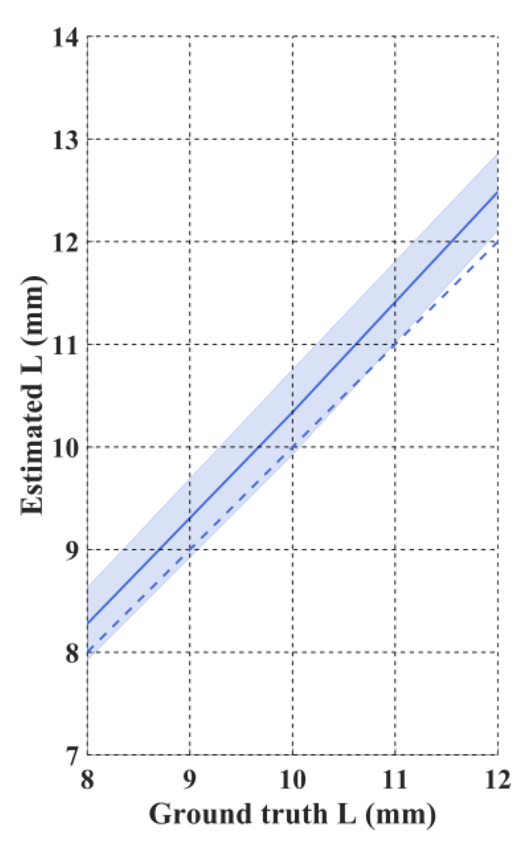
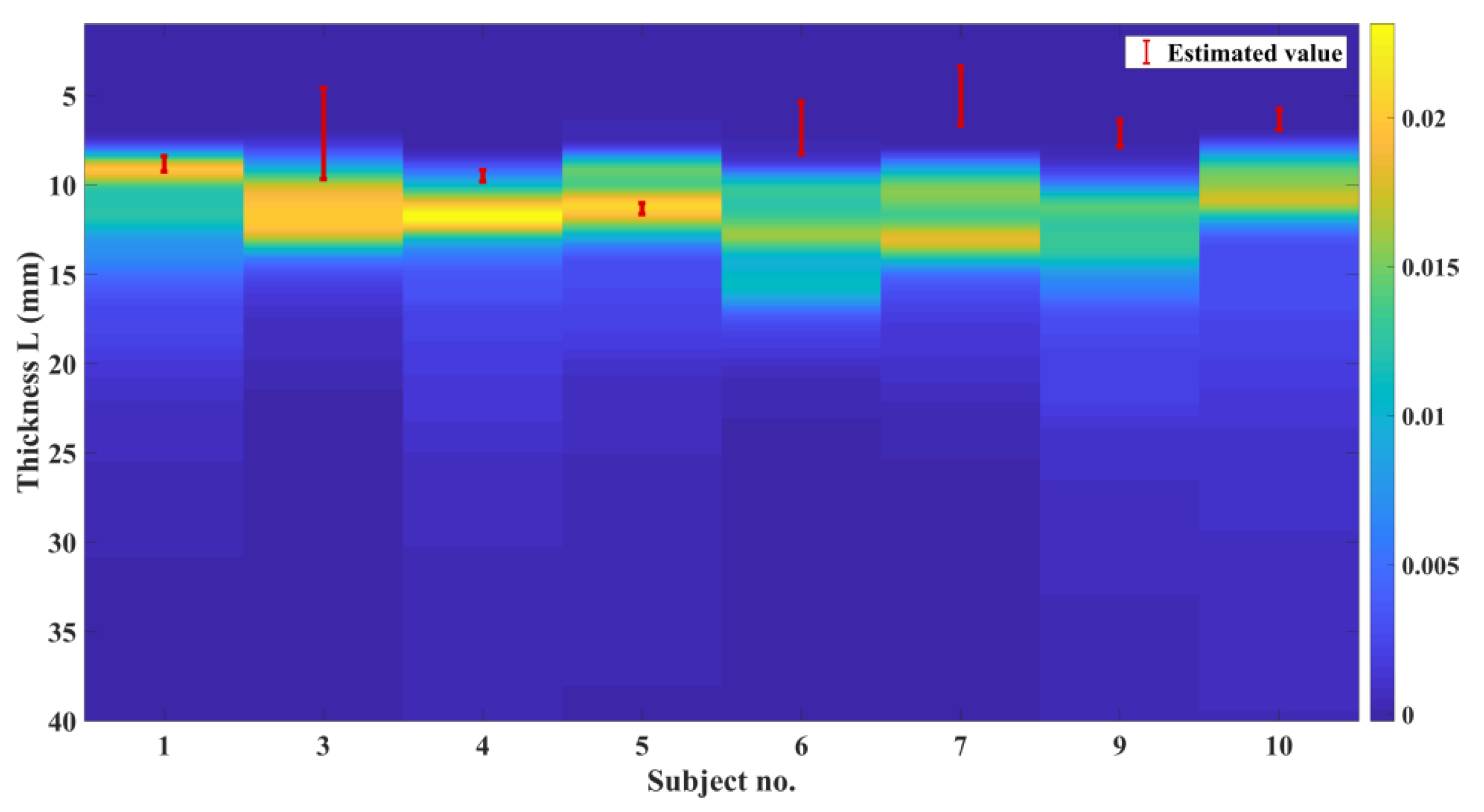
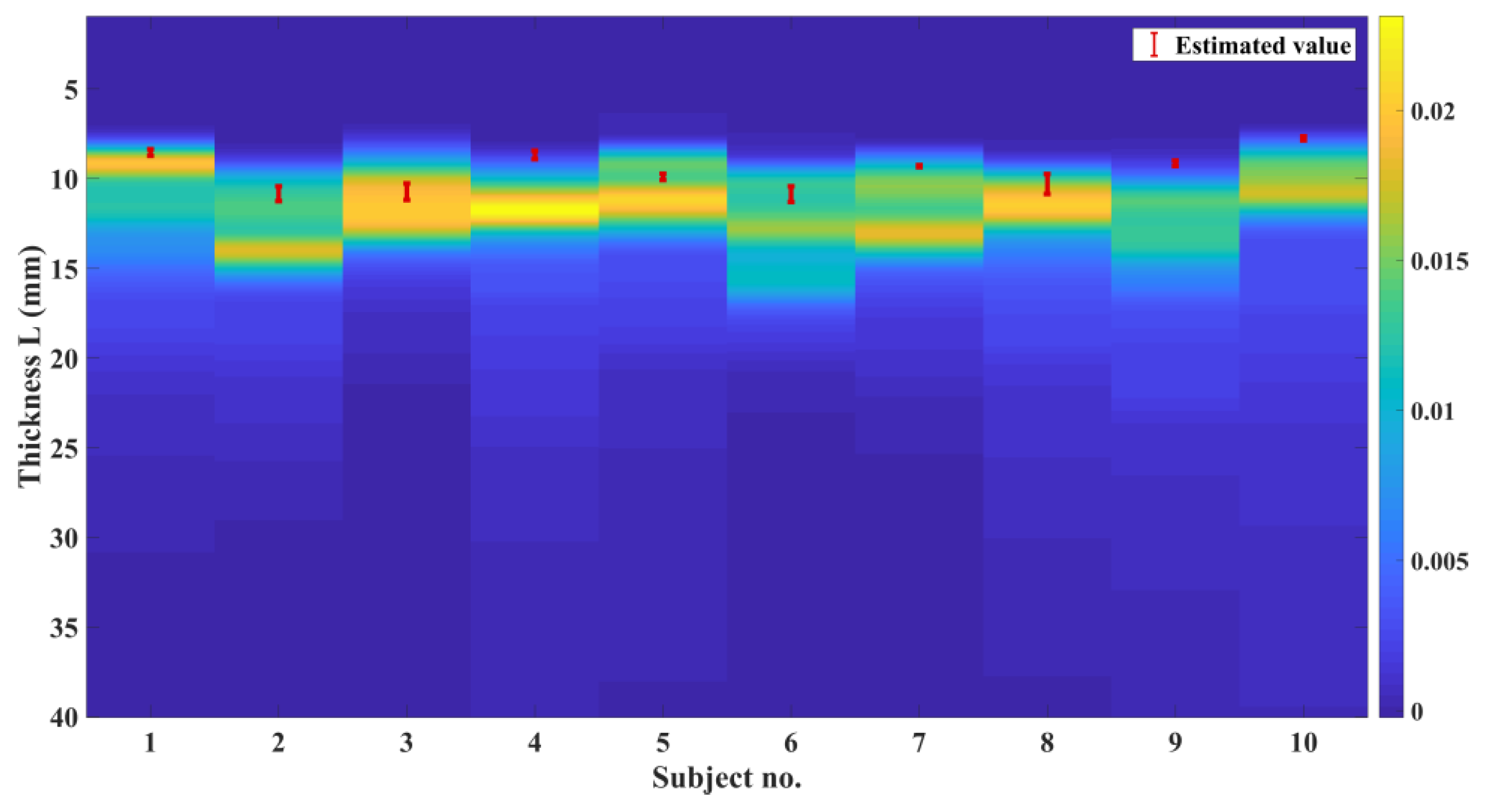
These results demonstrate that for the data corresponding to a head model, the proposed algorithm with a semi-infinite recovery-model estimates the TOI with an average recovery error of 8.4% with the two-layered recovery approach as compared to the error of 9.3% with the homogenous approach. Recovery of other tissue parameters (except for scattering power) can be achieved within 45.4% error with the two-layered approach as compared to the error of 48.3% with the homogenous recovery approach. However, using an appropriate recovery model (head-based model) the parameter recovery can be greatly improved by reducing the average recovery error of TOI to 4.2% with the two-layered approach as compared to the error of 9.8% with the homogenous approach, and the recovery of other tissue parameters (except for scattering power) can be achieved within 23.3% error with the two-layered approach as compared to the error of 37.8% with the homogenous recovery approach. However, the scattering power parameter exhibits relatively higher recovery errors due to its low sensitivity to light-intensity. In regard of the extra-cerebral tissue thickness, as the ground-truth is not a single value but rather varies spatially, we can quantify this variation in terms of a probability density functions as shown in Figure 9 & Figure 10, and by considering the tissue thickness at the peak probability as the ground-truth, the semi-infinite recovery model estimates the tissue thickness with an average error of 30.1%, whereas using an appropriate head based recovery model the error in estimating the tissue thickness is reduced to 11.8%.

4.3. NIRS on Forehead: Experimental Results

A broadband white-light tungsten-halogen light source is used along with a spectrometer to demonstrate the applicability of the described method using real NIRS data measured on a healthy subject at rest. A single subject was recruited from the University of Birmingham community, and written informed consent was obtained. A Tungsten-Halogen light source (Ocean optics HL-2000-FHSA, with approximately 5 minutes of stabilization time) is connected to an optical fiber and used as the source placed on the forehead of the subject. Another fiber as connected to a spectrometer (Ocean optics Flame-S) is used as the detector placed on the forehead of the subject at a distance 10, 20, 30, 40 mm away from the source. The 50 mm measurement was not used due to its low SNR. The two fibers (Ocean Optics: QP1000-2-VIS-BX) utilized in this experiment have a 1000 μm core diameter, with the efficient wavelength range from 300-1100 nm. The spectrometer consists of an entrance slit of 200 μm, and a grating with groove density of 600 grooves per mm. The signal is collected over different acquisition times of 30 ms, 1.5 s, 15 s, and 30 s, for the source-detector distances of 10, 20, 30 and 40 mm respectively, to obtain a good SNR. The collected signal is time-averaged by normalizing each measurement by its corresponding acquisition time. The spectrometer measures the intensities from 340 nm to 1015 nm at a spectral resolution of 0.3 nm, which is later down-sampled to a resolution of 10 nm by averaging every 33 (10/0.3) spectral data points, and is then cropped to the wavelength range 650 nm to 850 nm to match with measurement model considered in simulations. The intensity measurements at different source-detector distances were measured sequentially (starting from 10 mm to 40 mm) due to instrumental limitations. The subject is at rest during the measurements for all experiments. Each experiment was performed once a day with no stimuli and the subject position and data acquisition protocol was kept constant for all measurements, and therefore it was assumed that the hemodynamic changes over the entire duration of measurements (approx. 3 to 5 mins) were insignificant as often seen during the base-line measurements [23] while the subject is at rest. The proposed head-based recovery method as described in Section 4.2 was implemented using the boundary information of the forehead obtained from the MRI of the subject, and later the layer-1 thickness and tissue parameters of two layers were obtained. It should be noted that, while the MRI of the subject was obtained in a supine position, and the subject was measured while sitting on a chair at rest during the experiment and the position was kept constant for all measurements. As the anatomical boundary information of the subject comes from the thin skin/scalp tissue situated on the rigid structure of skull which is unaffected by the subject posture, the boundary information remains the same between the measurements and the acquired MRI. The NIRS experiment is repeated on three different days and the recovery of the parameters are as shown in

Table 4. Homogenous and two-layered parameters recovered using the head-based recovery method described in Section 4.2.

		Day-1	Day-2	Day-3
		Head-based recovery model	Head-based recovery model	Head-based recovery model
HbO (mM)	Homogenous	0.0697	0.0520	0.0694
	Layer-1	0.0358	0.0439	0.0563
	Layer-2	0.1116	0.1333	0.1567
Hb (mM)	Homogenous	0.0201	0.0145	0.0199
	Layer-1	0.0075	0.0098	0.0138
	Layer-2	0.0699	0.1017	0.1130
TOI (%)	Homogenous	77.6	78.2	77.7
	Layer-1	82.6	81.7	80.3
	Layer-2	61.4	56.7	58.1
Sa (mm-1)	Homogenous	0.44	0.56	0.44
	Layer-1	0.58	0.51	0.43
	Layer-2	0.34	0.24	0.12
Sp	Homogenous	0.64	0.69	0.65
	Layer-1	0.69	0.68	0.65
	Layer-2	1.07	1.26	3.0
L (mm)	Layer-1	9.9	10.7	10.8

. Although the physiological parameters of the tissue may have changed over different days, consistent values of tissue thickness over three days were recovered to ascertain the repeatability of the proposed method.

5. Discussion

A hyperspectral continuous wave NIRS parameter recovery method is presented to distinguish extra-cerebral and cerebral tissue hemodynamics, by separating the tissue absorption and scattering parameters and also by simultaneously fitting for the superficial layer thickness. Major challenges of continuous wave NIRS system have been the recovery of scatter (i.e., separating absorption and scattering information from the measured NIRS signal), and removing/separating the extra-cerebral tissue contamination from the NIRS signal to estimate the cerebral hemodynamics. It is shown theoretically in Section 2 that, while for a given spectral derivative of intensity measurements (any derivative measurements) have non-unique solution sets of layered tissue parameters, the absolute intensity measurements have a unique solution set of layered tissue parameters. A two-step approach is presented to recover the two-layered properties along with tissue thickness. In the case of data generated on a two-layered semi-infinite model, the proposed two step approach using a semi-infinite model in the inverse problem is shown to recover the tissue parameters within 16.6% errors. The recovery error of layer-1 properties are reduced with increasing thickness, this is because of the assumption in step-1 that the short distance measurement is only influenced by layer-1. This increase in accuracy of the estimation of layer-1 properties in step-1 which increase with thickness, should improve the recovery of layer-2 properties in step-2 but with increased thickness there is a drop in the sensitivity of layer-2 and therefore a similar trend of improvement in accuracy is not seen for layer-2. The opposite sign of mean-relative errors for absorption (i.e., HbO and Hb) and scattering parameters (scattering amplitude) shows that the cross-talk between these parameters is negatively related, any over-estimation of absorption is accompanied by an under-estimation of scattering amplitude and vice versa.

In the case of data generated on head models, a semi-infinite recovery model is shown to recover results with mixed accuracy. This is due to the complex structure i.e., the spatially varying curvature of external medium boundary and internal regional boundary. This is evident from the recovery accuracy of tissue thickness in Figure 9 for some head models where a correct two-layered semi-infinite model approximation wasn’t found. Therefore, to tackle this problem, using an appropriate boundary structure with the similar two-step parameter recovery approach, it has been demonstrated that the accuracy is greatly improved and similar to the initial case where the data is generated and recovered on semi-infinite model.

The practical implementation of this method has been shown in Section 4.3. The results presented in Table 4 show that the variation in tissue oxygenation levels recovered over three different days is less than 5%, and the variation in the recovery of extra-cerebral tissue thickness was not more than ~1mm, which clearly demonstrates the repeatability of the recovery algorithm.

It is important to highlight that the human head consists of multiple layers, such as skin, skull, CSF and brain tissue. Therefore, although the proposed methodology only assumes a two-layer model, to account for superficial signal contamination, the results indicate that this is much more suitable and robust as compared to the conventional homogenous assumptions. Future work should be directed towards extending this methodology to account for multiple layers, which may require the utilization of more boundary measurements and data-types to better extract information about pathlength [10].

6. Conclusions

A two-layered parameter recovery method using multi-distance hyper-spectral CW intensity measurements is proposed and demonstrated to recover the absolute hemoglobin concentrations, scattering parameters, and the superficial tissue thickness of a human head through simulations across different head models corresponding to different subjects. A practical implementation of this approach with real human subject data measured on the forehead is presented and has shown good repeatability in the recovered tissue parameters over three days. However, validation of these results is challenging as the absolute tissue parameters are unknown. It is the subject of future studies and needs further investigation. Finally, this work suggests the ability of multi-distance CW hyper-spectral data to retrieve or separate the extra-cerebral tissue parameters and the cerebral tissue parameters and that such an approach is more accurate than recovering bulk tissue parameters.

References

- Nollert, G.; Möhnle, P.; Tassani-Prell, P.; Uttner, I.; Borasio, G.D.; Schmoeckel, M.; Reichart, B. Postoperative Neuropsychological Dysfunction and Cerebral Oxygenation During Cardiac Surgery. Thorac. Cardiovasc. Surg. 1995, 43, 260–264. [Google Scholar] [CrossRef]
- Plessis, A.J.D. Cerebral oxygen supply and utilization during infant cardiac surgery. Ann. Neurol. 1995, 37, 488–497. [Google Scholar] [CrossRef] [PubMed]
- Scholkmann, F. A review on continuous wave functional near-infrared spectroscopy and imaging instrumentation and methodology. Neuroimage 2014, 85, 6–27. [Google Scholar] [CrossRef] [PubMed]
- Matcher, S.J. Absolute quantification methods in tissue near-infrared spectroscopy. Int. Soc. Opt. Photonics 1995, 2389, 486–495. [Google Scholar]
- Patterson, M.S.; Schwartz, E.; Wilson, B.C. Quantitative Reflectance Spectrophotometry For The Noninvasive Measurement Of Photosensitizer Concentration In Tissue During Photodynamic Therapy. Int. Soc. Opt. Photonics 1989, 1065, 115–122. [Google Scholar]
- Suzuki, S. Tissue oxygenation monitor using NIR spatially resolved spectroscopy. Int. Biomed. Opt. Symp. 1999, 3597, 582–592. [Google Scholar]
- Veesa, J.D.; Dehghani, H. Spectrally constrained approach of spatially resolved spectroscopy: towards a better estimate of tissue oxygenation. Opt. Soc. Am. 2018, 3, 37. [Google Scholar]
- Gagnon, L. Further improvement in reducing superficial contamination in NIRS using double. Neuroimage 2014, 85, 127–135. [Google Scholar] [CrossRef]
- Zeff, B.W. Retinotopic mapping of adult human visual cortex with high-density diffuse optical tomography. Proc. Natl. Acad. Sci. USA 2007, 104, 12169–12174. [Google Scholar] [CrossRef] [Green Version]
- Hallacoglu, B.; Sassaroli, A.; Fantini, S. Optical Characterization of Two-Layered Turbid Media for Non-Invasive, Absolute Oximetry in Cerebral and Extracerebral Tissue. PLoS ONE 2013, 8, e64095. [Google Scholar] [CrossRef]
- Li, A. Method for recovering quantitative broadband diffuse optical spectra from layered media. Appl. Opt. 2007, 46, 4828–4833. [Google Scholar] [CrossRef]
- Pucci, O.; Toronov, V.; Lawrence, K.S. Measurement of the optical properties of a two-layer model of the human head using broadband near-infrared spectroscopy. Appl. Opt. 2010, 49, 6324–6332. [Google Scholar] [CrossRef] [PubMed]
- Arridge, S.R.; Lionheart, W.R. Nonuniqueness in diffusion-based optical tomography. Opt. Lett. 1998, 23, 882–884. [Google Scholar] [CrossRef] [Green Version]
- Corlu, A. Uniqueness and wavelength optimization in continuous-wave multispectral diffuse optical tomography. Opt. Lett. 2003, 28, 2339–2341. [Google Scholar] [CrossRef] [PubMed]
- Dehghani, H. Near infrared optical tomography using NIRFAST: Algorithm for numerical model and image reconstruction. Commun. Numer. Methods Eng. 2008, 25, 711–732. [Google Scholar] [CrossRef]
- Kienle, A. Noninvasive determination of the optical properties of two-layered turbid media. Appl. Opt. 1998, 37, 779–791. [Google Scholar] [CrossRef] [PubMed]
- Pucci, O.; Sharieh, S.; Toronov, V. Spectral and spatial characteristics of the differential pathlengths in non-homogeneous tissues. SPIE BiOS 2008, 6855, 685506. [Google Scholar]
- Yalavarthy, P.K. Weight-matrix structured regularization provides optimal generalized least-squares estimate in diffuse optical tomography. Med. Phys. 2007, 34, 2085–2098. [Google Scholar] [CrossRef]
- Dehghani, H. Depth sensitivity and image reconstruction analysis of dense imaging arrays for mapping brain function with diffuse optical tomography. Appl. Opt. 2009, 48, 137–143. [Google Scholar] [CrossRef]
- Strangman, G.; Franceschini, M.A.; Boas, D.A. Factors affecting the accuracy of near-infrared spectroscopy concentration calculations for focal changes in oxygenation parameters. Neuroimage 2003, 18, 865–879. [Google Scholar] [CrossRef]
- Greisen, G.; Leung, T.; Wolf, M. Has the time come to use near-infrared spectroscopy as a routine clinical tool in preterm infants undergoing intensive care? Philos. Trans. R. Soc. A Math. Phys. Eng. Sci. 2011, 369, 4440–4451. [Google Scholar] [CrossRef] [PubMed] [Green Version]
- Tosh, W.; Patteril, M. Cerebral oximetry. BJA Educ. 2016, 16, 417–421. [Google Scholar] [CrossRef]
- Davies, D.J. Frequency-domain vs continuous-wave near-infrared spectroscopy devices: a comparison of clinically viable monitors in controlled hypoxia. J. Clin. Monit. Comput. 2017, 31, 967–974. [Google Scholar] [CrossRef] [PubMed]
Figure 1.
Schematic showing a two-layered medium.
Figure 2.
1st Spectral derivative of intensity data at = 1 and 0.5.
Figure 3.
Intensity data at = 1 and 0.5.
Figure 4.
Schematic showing semi-infinite model with source-detector locations on the boundary.
Figure 5.
Estimated tissue oxygenation index (TOI) values from the homogenous and two-layered parameter recovery methods corresponding to a two-layered semi-infinite medium of Layer-1 thickness as (a) 8 mm, (b) 10 mm, and (c) 12 mm, using multi-distance hyper-spectral continuous wave (CW) data. The ground-truth values of layer-1 and layer-2 is shown by dashed lines. The shaded region shows the standard deviation of recovery for different scattering parameters.
Figure 6.
Estimated Layer-1 thickness from the two-layered parameter recovery method using multi-distance hyper-spectral CW data. The shaded region shows the standard deviation of recovery for different scattering parameters of both layers and different TOI values of layer-2.
Figure 7.
Schematic showing an example of the head model with source-detectors placed on the forehead.
Figure 8.
Homogenous and two-layered recovery of TOI for two-layered head model based on: (a) semi-infinite recovery model, (b) head-based recovery model. The shaded region shows the standard deviation over different head models with different scattering parameters.
Figure 9.
Estimated values of layer-1 thickness with semi-infinite recovery model corresponding to extra-cerebral tissue for 10 subject head models, along with the ground-truth probability density function of extra-cerebral tissue thickness in the region of interest. Subjects 2, 8 are not shown as the algorithm did not converge to a stable solution.
Figure 10.
Estimated values of extra-cerebral tissue thickness with head-based recovery model for 10 subject head models, along with the ground-truth probability density function of extra-cerebral tissue thickness in the region of interest.