Deep CNN for IIF Images Classification in Autoimmune Diagnostics


Department of Physics and Chemistry, University of Palermo, 90128 Palermo, Italy
*
Author to whom correspondence should be addressed.
Appl. Sci. 2019, 9(8), 1618; https://doi.org/10.3390/app9081618
Submission received: 12 March 2019
/
Revised: 8 April 2019
/
Accepted: 15 April 2019
/
Published: 18 April 2019
(This article belongs to the Section Applied Biosciences and Bioengineering)
Abstract
:The diagnosis and monitoring of autoimmune diseases are very important problem in medicine. The most used test for this purpose is the antinuclear antibody (ANA) test. An indirect immunofluorescence (IIF) test performed by Human Epithelial type 2 (HEp-2) cells as substrate antigen is the most common methods to determine ANA. In this paper we present an automatic HEp-2 specimen system based on a convolutional neural network method able to classify IIF images. The system consists of a module for features extraction based on a pre-trained AlexNet network and a classification phase for the cell-pattern association using six support vector machines and a k-nearest neighbors classifier. The classification at the image-level was obtained by analyzing the pattern prevalence at cell-level. The layers of the pre-trained network and various system parameters were evaluated in order to optimize the process. This system has been developed and tested on the HEp-2 images indirect immunofluorescence images analysis (I3A) public database. To test the generalisation performance of the method, the leave-one-specimen-out procedure was used in this work. The performance analysis showed an accuracy of 96.4% and a mean class accuracy equal to 93.8%. The results have been evaluated comparing them with some of the most representative works using the same database.
1. Introduction
Antinuclear antibodies (ANAs) are a very large category of autoantibodies, or antibodies that the body produces against itself. They are related to many autoimmune diseases [1].
There are several laboratory investigations for the research and differentiation of antibodies to the nucleus. The most commonly used technique is indirect immunofluorescence, which uses a substrate of HEp-2 cells, that is, human epithelial type 2 cells, to detect antibodies to the nucleus. These particular cells show a very high nucleus/cytoplasm ratio and, by virtue of their neoplastic nature, present numerous mitotic figures allowing the operator to identify antibodies directed against the cellular antigens expressed during the mitotic phase. The ANA research is the first level test in the diagnosis of systemic autoimmune diseases, linked to an altered regulation of immune tolerance control mechanisms and characterized by the production of antibodies directed against cellular components that are no longer recognized as “self”.
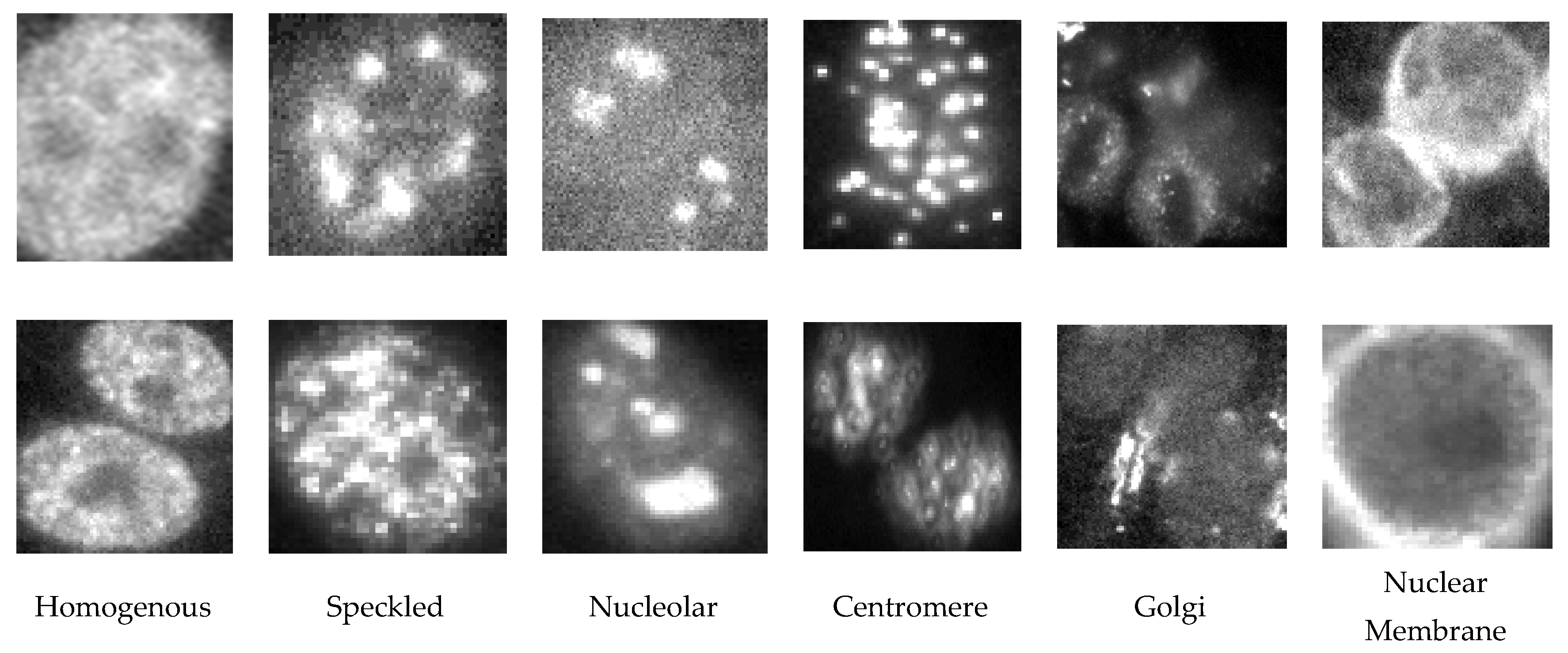
Indirect immunofluorescence (IIF) is the reference method for the determination of ANAs. Despite recent progress in the standardization of the indirect immunofluorescence method (automation of the analytical procedure), the technique still presents some methodological and interpretative limitations [2,3]. The importance of autoimmune diseases and the need for their early diagnosis has pushed the interest of manufacturers and the research world to develop expert fluoroscopic classification systems [4,5,6,7,8]. Figure 1 shows some examples of fluoroscopic patterns. As evinced in the figure, some patterns could be easily misidentified (i.e., homogeneous vs speckled).
In Benammar et al. [9] this difficulty of interpretation has been quantified by finding the percentage of concordance between the classifications of two senior immunologists; the analysis on 589 wells, both positive (six types of patterns) and negative, showed a concordance of around 71%.
Automatic systems to support diagnosis and in particular computer-aided diagnosis (CAD) systems are widely used for different tasks within medicine such as second reading, increasing the diagnosis speed, training physicians for special task, etc. [10,11].
In the last few years, the interest of the scientific community in the problem of HEp-2 cells classification or staining pattern recognition has been remarkable. This was also due to various contests that were organized on the topic [12,13,14], and to the availability of the first public databases [15,16].
In the work of Manivannan et al. [17] the authors extracted sets of local features that were aggregated through sparse encoding. They used a pyramidal decomposition of the cell that consisted in the central part and in the crown that contains the cell membrane. Linear support vector machines (SVMs) are the classifiers used on the learned dictionary; specifically, they used four SVMs, the first trained on the orientation of the original images and the remaining three on the images rotated 90, 180 and 270 degrees, respectively. With this technique they won the indirect immunofluorescence images analysis (I3A) competition in the International Conference on Pattern Recognition (ICPR) 2014.
Larsen et al. [18] developed a multiscale method using shape index histograms. The decomposition was spatial and presented a radially symmetric pattern. Second-order descriptors of textural type were extracted from the decompositions using a shape index. Finally, the shape index statistics were collected in histograms. The system was trained and tested on data from the I3A Task-1 public database.
Ensafi et al. [19] used a variant of the superpixel approach to extract patches from cells in combination with the sparse codes scheme. The features were extracted from both the superpixel patches and their boundary (high gradient zones). From the patches, features wer extracted using scale-invariant feature transform (SIFT) and speeded up robust feature (SURF) to form a dictionary learning. With the sparse codes, a multiclass linear SVM with a one-versus-all strategy is used.
In the work of Gragnaniello et al. [20] the authors used local descriptors at different scales and invariant to rotation. The descriptors were obtained from a log-polar grid transformation, from a multiscale smoothing of directional gradients, and from the Fourier transform. The bag of words technique was used in combination with a linear SVM. The I3A Task-1 database was used by the authors.
Xu et al. [21] presented a method based on linear local distance coding in which, starting from local features, a local distance vector transformation was used by Euclidean distance. Finally, linear coding and max pooling were used, both on the local distance vector and on the local features. The concatenations were provided as examples to a linear SVM.
In recent scientific research on pattern recognition, deep learning methods and in particular the convolutional neural networks (CNNs) have been proven to be efficient and reliable models to achieve remarkable performance for image classification and object detection tasks [22]. Moreover, it has been demonstrated that pre-trained CNN architectures can play an important role as feature extractors and allow high classification performance.
Very recently, depth learning methods have been applied to IIF image classification problems. In the work of Li Y. et al. [23] the authors addressed the problem of segmentation and classification of IIF images. In particular, they used a variant of the note VGG-16 (16-layer network used by the VGG team) called FCN which is aimed at segmentation. They used CNNs for both segmentation and classification. For the development and the performance test, they used the I3A Task-2 database.
Gupta et al. [24] used the known CNN AlexNet in combination with an SVM classifier for the classification of cells in mitosis.
In our previous work [25] we addressed the problem of intensity fluorescence classification. The problem was faced by analyzing the whole image and starting from it by extracting the features. To this end, several pre-trained networks, used as feature extractors, were analyzed, and the image classification was obtained by training an SVM classifier.
Oraibi et al. [26] used the known CNN VGG-19 to extract features and combine them with local features such as RIC-LBP (rotation invariant co-occurrence local binary pattern) and JML (joint motif labels) for an efficient cell classification. The combination of features was used to train a random forest classifier.
Li H. et al. [27] proposed a method for analyzing HEp-2 images based on the use of a CNN to construct a pattern histogram, and through this a linear SVM was trained. The CNN used was composed of 10 layers, of which the first nine were convolutional layers while the last was a softamax layer for classification. The system was trained and tested on data from the I3A Task-2 public database.
In the present paper a system able to classify the fluorescence patterns is presented. The analysis was conducted both at the cell-level (i.e., in terms of cell images correctly classified) and at image-level (i.e., in terms of IIF images correctly classified). The system uses a pre-trained network, AlexNet [28], as a feature extractor and is able to classify the following six fluoroscopic patterns: Homogeneous, speckled, nucleolar, centromere, Golgi, and nuclear membrane. The classification phase was carried out by developing six linear SVM classifiers with a one-against-all training scheme (OAA). The cell-pattern association was obtained by means of a k-nearest neighbors (KNN) classifier. Furthermore, in the present work, the effectiveness of the extraction of the features both from the segmented cells (internal) and from the boundary boxes containing the cells was evaluated. The data augmentation method as a tool for improving classification performance was evaluated. Finally, different layers of the best known and used pre-trained network were evaluated as feature extractors for the problem of the classification of HEp-2 image patterns. For an effective performance comparison, the method was evaluated on a public data set issued by the 2014 ICPR Competition [14].
2. Materials and Methods
2.1. Database and Statistics
In this study the publicly available dataset Task-1 from the I3A Contest [14] was used.
The HEp-2 images Database I3Asel were made public in the “Contest on Performance Evaluation on Indirect Immunofluorescence Image Analysis Systems”, hosted by the 22th International Conference on Pattern Recognition (ICPR 2014). The dataset was collected between 2011 and 2013 at Sullivan Nicolaides Pathology laboratory, Australia. The competition was based on two tasks: Task-1 on HEp-2 pre-segmented cells classification, and Task-2 on well images classification.
In Task-1, it was necessary to identify six straining patterns (homogeneous, speckled, nucleolar, centromere, Golgi, nuclear membrane). The total number of cells was 13,596, extracted from 83 specimens.
Table 1 shows the pattern distribution of the images provided for Task-1.
The specimens were automatically photographed using a monochrome high dynamic range cooled microscopy camera which was fitted on a microscope with a plan-Apochromat 20x/0.8 objective lens and an LED illumination source.
The labelling process involved at least two scientists who read each patient specimen under a microscope. A third expert’s opinion was sought to adjudicate any discrepancy between the two opinions. They used each specimen label for the ground truth of cells extracted from it. Furthermore, all the labels were validated by using secondary tests such as ENA (extractable nuclear antigens) and anti-dsDNA (Anti-double stranded DNA antibody) in order to confirm the presence and/absence of specific patterns.
It is known that in a supervised training, in order not to invalidate the classification result, it is necessary that the test does not contain examples used in training [29,30]. In our specific case, since cells belonging to the same image have a very similar informative contribution, it is advisable, in order not to distort the performance result on the test, that if cells of an image are used in training, no cell of the same image, let alone examples obtained from these for data augmentation, is present in the test. For these reasons, the procedure called leave-one-specimen-out (LOSO) was used in this work [31]. In the LOSO strategy, each time all cell images (and the relative images obtained by data augmentation) from one of the 83 specimens are used for testing, the rest are used for training. Since 83 different specimens were available, we used images from 82 specimens for training in each fold. In this work, the statistical analysis of system performance was based on accuracy and mean class accuracy (MCA) of classification [32] defined as follows:
where CCRk is the correct classification rate for class k determined as follows:
2.2. System Workflow
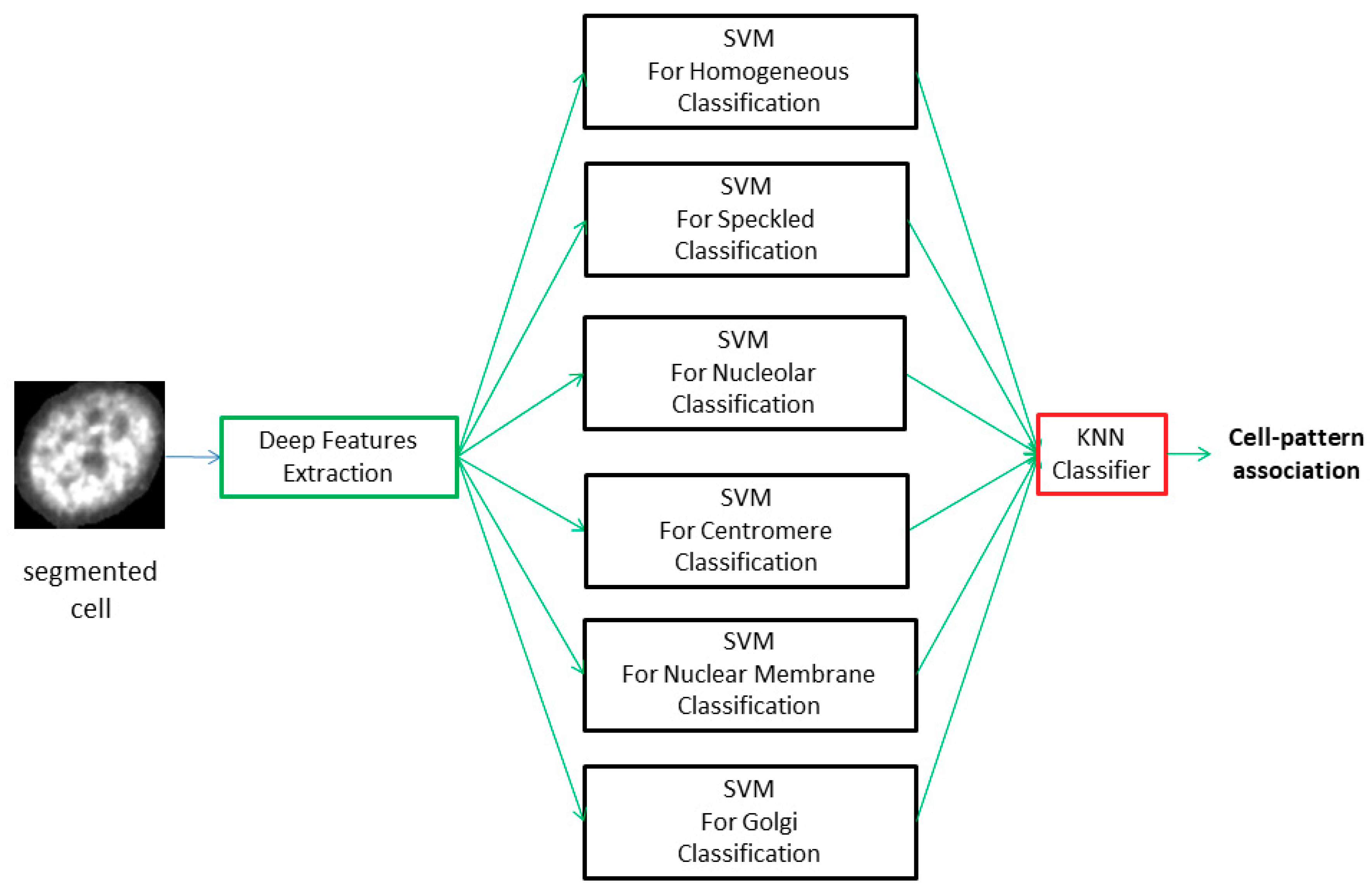
Figure 2 shows the flow of operations adopted in this work for cellular classification: The generic segmented region of interest (ROI) is decomposed by the multilayer neural network to obtain the features used as inputs of the six SVMs. The six output values obtained from the six binary classifiers represent how much the generic region “resembles” each of the analyzed pattern classes. The image classification is achieved by means of the cell classification. Indeed, the classification at the image-level was obtained by analyzing the prevalence of the patterns at the cell-level and associating the generic image to the pattern with the highest rate.
The choice of best features and parameters was performed automatically, using the mean class accuracy as a figure of merit.
To verify the classification power contained in the region immediately adjacent to the cell, in addition to the segmentation mask, the boundary box containing the cell was also analyzed and the relative performance results were obtained.
2.3. Data Preparation
In order to reduce the intensity variability present in the database, a contrast stretching was performed, defined as follows:
where I and Ic denote respectively the images after and before the transformation, and min and max represent the minimum and maximum intensity of input image, respectively. Since the images are stored in 8 bits the normalization is referred to the maximum possible value, that is, 255.
Furthermore, to increase the number of training examples, a data augmentation was made. In particular, an increase for rotation of cell images at angles of 20° was achieved; overall, a multiplication of the data by a factor of 18 was obtained. Data augmentation is a very effective practice especially when the data set for training is limited, or as in our case, when some classes are not particularly represented in the set of examples. The effect of this data augmentation was valued quantitatively in terms of performance.
2.4. Deep CNN
In recent years, deep learning networks have allowed significant improvements in classification performance for many problems of pattern recognition and in fact representing in many areas the state of the art of research.
The term “deep” usually refers to the number of layers hidden in the neural network. Traditional neural networks contain only one to two hidden layers, while deep networks can contain up to 150. Deep learning models are trained using large labeled data sets and neural network architectures that learn features directly from data without having to manually extract them.
One of the most common types of neural networks is known as a convoluted neural network (CNN or ConvNet). A CNN conveys the characteristics learned with the input data and uses the convolutional layers in 2D, which make this architecture suitable for 2D data processing, such as images. CNNs eliminate the need for manual feature extraction [33,34,35,36,37], so the user does not have to identify features used for image classification. In fact, it is possible to use the power of the pre-trained networks, without investing time and effort in training, to implement the extraction phase of the characteristics. Feature extraction can be the fastest way to use in-depth learning. The operation of CNN is based on the extraction of the features directly from the images. The automatic extraction of the features allows a high precision of the deep learning models intended for artificial vision activities, such as the classification of objects.
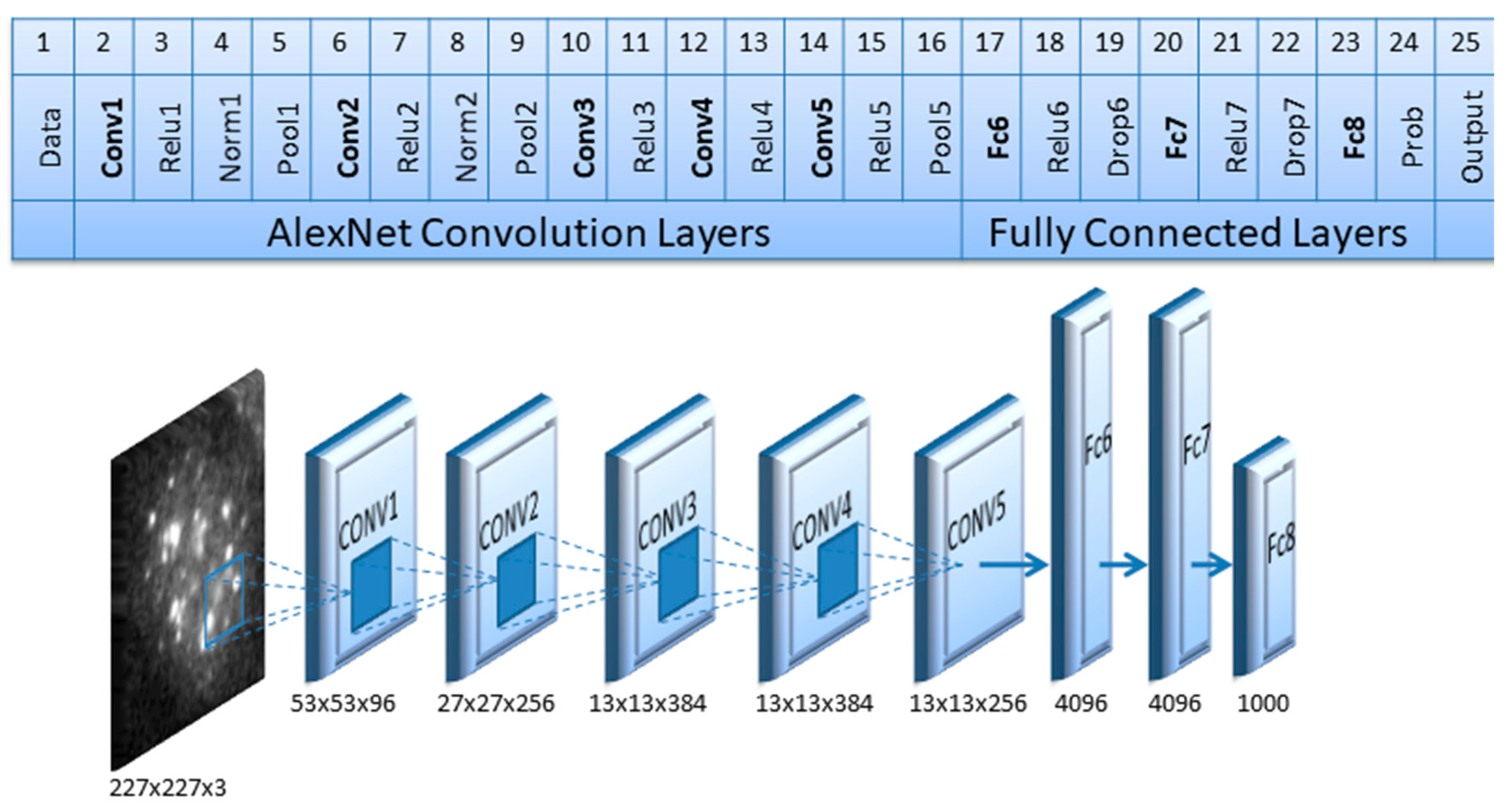
In this work it was decided to use one of the best known CNN (Convolutional Neural Network) networks: AlexNet [28]. This network was trained on the ImageNet database [38] consisting of more than a million images with 1000 object categories. The architecture of the pre-trained network used is shown in Figure 3. The peculiar characteristics of this network are briefly described below: The network architecture consists of eight layers of depth. The first layer accepts an RGB input image of size 227 × 227. The first five layers are convolutional (some of which are followed by max-pooling layers) while the last three are fully connected layers with a final 1000-way softmax. AlexNet uses a ReLU (rectified linear unit) layer that consists of a simple activation function such as the max(0,x) thresholding at zero that is faster than the traditional sigmoid. Furthermore, to avoid the problem of overfitting, dropout layers in the flully-connected layers are used as a regularization method.
Since the network has been weighed and trained to classify a large variety of objects, the feature representation is very robust. In particular, the first layers of the network express lower-level features that are gradually elaborated by the deeper layers, refining them into higher-level features. In this work, the sub-images containing the cells to be classified have been appropriately rescaled to acquire the correct dimensionality for the network entrance (227 × 227)
The vector of features extracted from the pretrainded CNN are used in the training of six support vector machine (SVM) of linear type as specified in Section 2.5. Different layers of the AlexNet network have been evaluated as feature extractors for the problem of the classification of HEp-2 image patterns and the best configuration has been identified.
2.5. Classification
In order to associate the generic image with the correct pattern class, the effectiveness of the characteristics extracted from the CNN has been used in input to the SVMs classifiers.
Since the problem to be addressed required a multiclass classification, we followed the OAA strategy which breaks down the multiclass problem into a series of binary classifiers. In this case, the classification of the six patterns to be identified was decomposed into six binary classifiers that consider the pattern i-th (with i between one and six) as the first class and the remaining five patterns as the second class of the relative binary classifier [39,40].
The choice of the SVM classifier is due to the possibility of this classifier to be implemented, and to allow good classification performance, even if there are few examples available [41,42,43,44,45,46]; this is possible because the SVM classifier has few parameters. In particular, six SVM classifiers with linear kernel were implemented, the simplest in terms of parameters to search. Matlab’s “logspace” function in the range between 10−6 and 101.5 was used as the parameter search method for the linear kernel; 11 equidistant values on a logarithmic scale were analyzed.
Usually in the OAA scheme, each example of the test is assigned to the majority pattern, that is, the pattern that has obtained the highest output value from the relative SVM. In this work the cell-pattern association was implemented by means of a KNN classifier using the outputs of the six SVMs; this choice, carried out because a summary of the classifications of each SVM contributes to improving the classification result, was analyzed in terms of performance. The classification at the image-level was obtained by analyzing the prevalence of the patterns at the cell-level and associating the generic image to the pattern with the highest rate.
3. Results
The performance of the method proposed here was obtained both at cell-level and at image-level. The best confusion matrix, obtained with the LOSO procedure on the 13,596 cell images present in the Task-1 database, is presented in Table 2.
The results contained in Table 2 have been summarized in Table 3 in order to highlight the per-class accuracy.
An overall accuracy of 81.93% and an MCA of 82.16%, at cell-level was achieved.
A performance analysis was performed to evaluate the classification power contained in the region immediately adjacent to the cell, using the boundary box containing the generic ROI rather than the segmentation mask. In this configuration the performances were slightly decreased and in particular the following were obtained: Accuracy = 80.3%, MCA = 79.9%.
The prevalence of patterns at the cell-level was analyzed and, for classification at the image-level, the generic image was associated to the most present pattern. Table 4 shows the confusion matrix at the image-level.
The mean class accuracy obtained was equal to 93.8%, while the accuracy achieved was equal to 96.4%. In the same configuration, the performance results without using the KNN classifier were: Accuracy = 94.0%, MCA = 91.5%.
Regarding the analysis of the features and the use of CNN, the best configuration of the method, which allowed us to obtain the confusion matrix of Table 4, made use of the 4096 features of the Fc7 layer. Table 5 shows the details of the performances obtained when the pre-trained network layer changes.
The best performances, at image-level, obtained without the phase of data augmentation were: Accuracy = 94.0%, MCA = 91.67%. For all the analyzed layers, when using the data augmentation there has always been an increase in performance; the magnitude of the increase was between 2% and 4%.
In order to have a clear comparison of the performances, Table 6 reports the values of accuracy, MCA and the training method used, for various CAD systems proposed in the recent literature and using the database I3A Task-1.
4. Discussion and Conclusions
In this work an automatic system, able to characterize IIF images in terms of fluorescent pattern which is critical for the diagnosis of autoimmune diseases, has been proposed.
The developed system was evaluated on a public database, consisting of 83 specimens (13,596 cell images) obtaining an overall accuracy of pattern classification around 96%.
The proposed system is based on the use of the well-known pre-trained AlexNet network. The AlexNet network was used in the convoluted neural network mode as a feature extractor. The different layers of the network were analyzed and the best was identified for the classification of fluorescence patterns.
The procedure for using the data in training/testing was the leave-one-specimen-out method. The data augmentation, carried out by rotations, led to a significant increase in performance; the less statistically present classes in the database such as the Golgi pattern benefited the most from the correct classification. Moreover, for the feature extraction, we could verify better performances in using the segmentation mask rather than the boundary box.
The results were evaluated by comparing them with some of the most representative works using the same public database. The results obtained show an excellent ability of the method to classify the patterns under analysis, despite the small number of specimens in the database. The method proposed here has shown better performance or in any case comparable with other methods of recent literature (including the winner of the last competition on the subject). Hence, the system here presented can be proposed as a valid solution to the problem of ANA testing automatization.
Author Contributions
D.C. conceived of the study, performed the statistical analysis and drafted the manuscript. V.T. developed the software, optimized the parameters and helped to write the draft. G.R. participated in the design and coordination of the manuscript.
Funding
This research received no external funding.
Conflicts of Interest
The authors declare no conflict of interest.
References
- Grygiel-Górniak, B.; Rogacka, N.; Puszczewicz, M. Antinuclear antibodies in healthy people and non-rheumatic diseases—Diagnostic and clinical implications. Reumatologia 2018, 56, 243–248. [Google Scholar] [CrossRef]
- Agmon-Levin, N.; Damoiseaux, J.; Kallenberg, C.; Sack, U.; Witte, T.; Herold, M.; Bossuyt, X.; Musset, L.; Cervera, R.; Plaza-Lopez, A.; et al. International recommendations for the assessment of autoantibodies to cellular antigens referred to as anti-nuclear antibodies. Ann. Rheum. Dis. 2014, 73, 17–23. [Google Scholar] [CrossRef]
- Bizzaro, N.; Antico, A.; Platzgummer, S.; Tonutti, E.; Bassetti, D.; Pesente, F.; Tozzoli, R.; Tampoia, M.; Villalta, D. Automated antinuclear immunofluorescence antibody screening: A comparative study of six computer-aided diagnostic systems. Autoimmun. Rev. 2014, 13, 292–298. [Google Scholar] [CrossRef] [PubMed]
- Hiemann, R.; Büttner, T.; Krieger, T.; Roggenbuck, D.; Sack, U.; Conrad, K. Challenges of automated screening and differentiation of non-organ specific autoantibodies on HEp-2 cells. Autoimmun. Rev. 2009, 9, 17–22. [Google Scholar] [CrossRef] [PubMed]
- Rigon, A.; Buzzulini, F.; Soda, P.; Onofri, L.; Arcarese, L.; Iannello, G.; Afeltra, A. Novel opportunities in automated classification of antinuclear antibodies on HEp-2 cells. Autoimmun. Rev. 2011, 10, 647–652. [Google Scholar] [CrossRef] [PubMed]
- Willitzki, A.; Hiemann, R.; Peters, V.; Sack, U.; Schierack, P.; Rödiger, S.; Anderer, U.; Conrad, K.; Bogdanos, D.P.; Reinhold, D.; et al. New platform technology for comprehensive serological diagnostics of autoimmune diseases. Clin. Dev. Immunol. 2012, 2012, 284740. [Google Scholar] [CrossRef] [PubMed]
- Vivona, L.; Cascio, D.; Taormina, V.; Raso, G. Automated approach for indirect immunofluorescence images classification based on unsupervised clustering method. IET Comput. Vis. 2018, 12, 989–995. [Google Scholar] [CrossRef]
- Cascio, D.; Taormina, V.; Cipolla, M.; Fauci, F.; Vasile, M.; Raso, G. HEp-2 Cell Classification with heterogeneous classes-processes based on K-Nearest Neighbours. In Proceedings of the IEEE 1st Workshop on Pattern Recognition Techniques for Indirect Immunofluorescence Images ICPR, Stockholm, Sweden, 24 August 2014; pp. 10–15. [Google Scholar]
- Elgaaied Benammar, A.; Cascio, D.; Bruno, S.; Ciaccio, M.C.; Cipolla, M.; Fauci, A.; Morgante, R.; Taormina, V.; Gorgi, Y.; Triki, R.M.; et al. Computer-assisted classification patterns in autoimmune diagnostics: The A.I.D.A. Project. Biomed Res. Int. 2016, 2016, 1–9. [Google Scholar] [CrossRef] [PubMed]
- Ciatto, S.; Cascio, D.; Fauci, F.; Magro, R.; Raso, G.; Ienzi, R.; Martinelli, F.; Simone, M.V. Computer-assisted diagnosis (CAD) in mammography: Comparison of diagnostic accuracy of a new algorithm (Cyclopus®, Medicad) with two commercial systems. Radiol. Med. 2009, 114, 626–635. [Google Scholar] [CrossRef]
- Cascio, D.; Fauci, F.; Iacomi, M.; Raso, G.; Magro, R.; Castrogiovanni, D.; Filosto, G.; Ienzi, R.; Vasile, M.S. Computer-aided diagnosis in digital mammography: Comparison of two commercial systems. Imaging Med. 2014, 6, 13–20. [Google Scholar] [CrossRef]
- Foggia, P.; Percannella, G.; Soda, P.; Vento, M. Benchmarking hep-2 cells classification methods. IEEE Trans. Med. Imaging 2013, 32, 1878–1889. [Google Scholar] [CrossRef]
- Foggia, P.; Percannella, G.; Saggese, A.; Vento, M. Pattern recognition in stained HEp-2 cells: Where are we now? Pattern Recognit. 2014, 47, 2305–2314. [Google Scholar] [CrossRef]
- Lovell, B.C.; Percannella, G.; Vento, M.; Wiliem, A. Performance Evaluation of Indirect Immunofluorescence Image Analysis Systems. In Proceedings of the ICPR Workshop, Stockholm, Sweden, 24 August 2014. [Google Scholar]
- Hobson, P.; Lovell, B.C.; Percannella, G.; Saggese, A.; Vento, M.; Wiliem, A. Computer Aided Diagnosis for Anti-Nuclear Antibodies HEp-2 images: Progress and challenges. Pattern Recognit. Lett. 2016, 82, 3–11. [Google Scholar] [CrossRef]
- Cascio, D.; Taormina, V.; Raso, G. An Automatic HEp-2 Specimen Analysis System Based on an Active Contours Model and an SVM Classification. Appl. Sci. 2019, 9, 307. [Google Scholar] [CrossRef]
- Manivannan, S.; Li, W.; Akbar, S.; Wang, R.; Zhang, J.; McKenna, S.J. An automated pattern recognition system for classifying indirect immunofluorescence images of HEp-2 cells and specimens. Pattern Recognit. 2016, 51, 12–26. [Google Scholar] [CrossRef] [Green Version]
- Larsen, A.B.L.; Vestergaard, J.S.; Larsen, R. Hep-2 cell classification using shape index histograms with donut-shaped spatial pooling. IEEE Trans. Med. Imaging 2014, 33, 1573–1580. [Google Scholar] [CrossRef] [PubMed]
- Ensafi, S.; Lu, S.; Kassim, A.A.; Tan, C.L. Accurate HEp-2 cell classification based on Sparse Coding of Superpixels. Pattern Recognit. Lett. 2016, 82, 64–71. [Google Scholar] [CrossRef]
- Gragnaniello, D.; Sansone, C.; Verdoliva, L. Biologically-Inspired Dense Local Descriptor for Indirect Immunofluorescence Image Classification. In Proceedings of the IEEE 1st Workshop on Pattern Recognition Techniques for Indirect Immunofluorescence Images ICPR, Stockholm, Sweden, 24 August 2014. [Google Scholar]
- Xu, X.; Lin, F.; Ng, C.; Leong, K.P. Automated classification for HEp-2 cells based on linear local distance coding framework. EURASIP J. Image Video Process. 2015, 2015, 13. [Google Scholar] [CrossRef]
- Chen, J.; Liu, Q.; Gao, L. Visual Tea Leaf Disease Recognition Using a Convolutional Neural Network Model. Symmetry 2019, 11, 343. [Google Scholar] [CrossRef]
- Li, Y.; Shen, L.; Zhouand, X.; Yu, S. HEp-2 Specimen Classification with fully convolutional network. In Proceedings of the 23rd International Conference on Pattern Recognition (ICPR), Cancun, Mexico, 4–8 December 2016. [Google Scholar]
- Gupta, K.; Bhavsar, A.; Sao, A.K. CNN based mitotic HEp-2 cell image detection. In Proceedings of the BIOIMAGING 2018—5th International Conference on Bioimaging, Funchal, Portugal, 19–21 January 2018. [Google Scholar]
- Cascio, D.; Taormina, V.; Raso, G. Deep Convolutional Neural Network for HEp-2 fluorescence intensity classification. Appl. Sci. 2019, 9, 408. [Google Scholar] [CrossRef]
- Oraibi, Z.; Yousif, H.; Hafiane, A.; Seetharaman, G.; Palaniappan, K. Learning local and deep features for efficient cell image classification using random forests. In Proceedings of the IEEE International Conference on Image Processing, Athens, Greece, 7–10 October 2018. [Google Scholar]
- Li, H.; Huang, H.; Zheng, W.-S.; Xie, X.; Zhang, J. HEp-2 Specimen Classification via Deep CNNs and Pattern Histogram. In Proceedings of the 23rd International Conference on Pattern Recognition (ICPR), Cancun, Mexico, 4–8 December 2016. [Google Scholar]
- Krizhevsky, A.; Sutskever, I.; Hinton, G.E. Imagenet classification with deep convolutional neural networks. Adv. Neural Inf. Process. Syst. 2012, 25, 1097–1105. [Google Scholar] [CrossRef]
- Manavalan, B.; Shin, T.H.; Lee, G. DHSpred: Support-vector-machine-based human DNase I hypersensitive sites prediction using the optimal features selected by random forest. Oncotarget 2017, 9, 1944–1956. [Google Scholar] [CrossRef] [PubMed]
- Manavalan, B.; Shin, T.H.; Lee, G. PVP-SVM: Sequence-Based Prediction of Phage Virion Proteins Using a Support Vector Machine. Front. Microbiol. 2018, 16, 476. [Google Scholar] [CrossRef] [PubMed]
- Li, H.; Zhang, J.; Zheng, W.-S. Deep CNNs for HEp-2 Cells Classification: A Cross-specimen Analysis. arXiv, 2018; arXiv:1604.05816. [Google Scholar]
- Cascio, D.; Taormina, V.; Cipolla, M.; Bruno, S.; Fauci, F.; Raso, G. A multi-process system for HEp-2 cells classification based on SVM. Pattern Recognit. Lett. 2016, 82, 56–63. [Google Scholar] [CrossRef]
- Wang, N.; Yeung, D.-Y. Learning a deep compact image representation for visual tracking. In Proceedings of the 26th International Conference on Neural Information Processing Systems, Lake Tahoe, Nevada, 5–10 December 2013; pp. 809–817. [Google Scholar]
- Iacomi, M.; Cascio, D.; Fauci, F.; Raso, G. Mammographic images segmentation based on chaotic map clustering algorithm. BMC Med. Imaging 2014, 14, 1–11. [Google Scholar] [CrossRef] [PubMed]
- Fauci, F.; La Manna, A.; Cascio, D.; Magro, R.; Raso, G.; Iacomi, M.; Vasile, M.S. A Fourier Based Algorithm for Microcalcifications Enhancement in Mammographic Images. In Proceedings of the IEEE Nuclear Science Symposium and Medical Imaging Conference, Dresden, Germany, 19–25 October 2008; pp. 4388–4391. [Google Scholar]
- Masala, G.L.; Golosio, B.; Cascio, D.; Fauci, F.; Tangaro, S.; Quarta, M.; Cheran, S.C.; Torres, E.L. Classifiers trained on dissimilarity representation of medical pattern: A comparative study. Nuovo Cimento- Societa Italiana di Fisica Sezione C 2005, 28, 905–912. [Google Scholar]
- Vivona, L.; Cascio, D.; Magro, R.; Fauci, F.; Raso, G. A fuzzy logic C-means clustering algorithm to enhance microcalcifications clusters in digital mammograms. In Proceedings of the Nuclear Science Symposium and Medical Imaging Conference (NSS/MIC) IEEE, Valencia, Spain, 23–29 October 2011; pp. 3048–3050. [Google Scholar]
- Russakovsky, O.; Deng, J.; Su, H.; Krause, J.; Satheesh, S.; Ma, S.; Huang, Z.; Karpathy, A.; Khosla, A.; Bernstein, M.; et al. ImageNet Large Scale Visual Recognition Challenge. IJCV 2015, 115, 211–252. [Google Scholar] [CrossRef] [Green Version]
- Furnkranz, J.; Round, R. Classification. J. Mach. Learn. Res. 2002, 2, 721–747. [Google Scholar]
- Hsu, C.-W.; Chang, C.-C.; Lin, C.-J. A Practical Guide to Support Vector Classification; Department of Computer Science National Taiwan University: Taipei, Taiwan, 2003. [Google Scholar]
- Manavalan, B.; Basith, S.; Shin, T.H.; Wei, L.; Lee, G. mAHTPred: A sequence-based meta-predictor for improving the prediction of anti-hypertensive peptides using effective feature representation. Bioinformatics 2018. [Google Scholar] [CrossRef]
- Wei, L.; Luan, S.; Nagai, L.A.E.; Su, R.; Zou, Q. Exploring sequence-based features for the improved prediction of DNA N4-methylcytosine sites in multiple species. Bioinformatics 2018. [Google Scholar] [CrossRef] [PubMed]
- Manvalan, B.; Basith, S.; Shin, T.H.; Choi, S.; Kim, M.O.; Lee, G. MLACP: Machine-learning-based prediction of anticancer peptides. Oncotarget 2017, 8, 77121–77136. [Google Scholar] [CrossRef] [PubMed]
- Wei, L.; Chen, H.; Su, R. M6APred-EL: A Sequence-Based Predictor for Identifying N6-methyladenosine Sites Using Ensemble Learning. Mol. Ther. Nucleic Acids 2018, 12, 635–644. [Google Scholar] [CrossRef] [PubMed]
- Manavalan, B.; Shin, T.H.; Kim, M.O.; Lee, G. PIP-EL: A New Ensemble Learning Method for Improved Proinflammatory Peptide Predictions. Front. Immunol. 2018, 9, 1783. [Google Scholar] [CrossRef] [PubMed]
- Wei, L.; Zhou, C.; Chen, H.; Song, J.; Su, R. ACPred-FL: A sequence-based predictor using effective feature representation to improve the prediction of anti-cancer peptides. Bioinformatics 2018, 34, 4007–4016. [Google Scholar] [CrossRef] [PubMed]
Figure 1.
Sample cells images of six patterns from different specimens.

Figure 2.
Flowchart of the proposed method for cell classification: The segmented region of interest (ROI) is decomposed by the multilayer neural network to obtain the features that are used as inputs of the six support vector machines (SVMs). The cell-pattern association is obtained with a k-nearest neighbors (KNN) classifier.

Figure 3.
AlexNet architecture used in this work for patterns classification.


Table 1.
Staining patterns distribution in Task-1 dataset.
| Homogeneous | Speckled | Nucleolar | Centromere | Golgi | Nuclear Membrane | |
|---|---|---|---|---|---|---|
| Cell Numbers | 2494 | 2831 | 2598 | 2741 | 724 | 2208 |
Table 2.
Confusion matrix of our method at cell-level.
| Homogenous | Speckled | Nucleolar | Centromere | Golgi | Nuclear Membrane | |
|---|---|---|---|---|---|---|
| Homogenous | 2194 | 215 | 7 | 21 | 36 | 21 |
| Speckled | 261 | 2328 | 91 | 57 | 83 | 11 |
| Nucleolar | 80 | 312 | 2077 | 45 | 66 | 18 |
| Centromere | 48 | 379 | 114 | 2144 | 53 | 3 |
| Golgi | 50 | 17 | 39 | 0 | 604 | 14 |
| Nuclear Membrane | 256 | 43 | 19 | 2 | 95 | 1793 |
Table 3.
Per-class accuracy.
| Class | Accuracy |
|---|---|
| Homogenous | 87.97% |
| Speckled | 82.23% |
| Nucleolar | 79.94% |
| Centromere | 78.21% |
| Golgi | 83.42% |
| Nuclear membrane | 81.20% |
Table 4.
Confusion matrix of our method at image-level.
| Homogenous | Speckled | Nucleolar | Centromere | Golgi | Nuclear Membrane | |
|---|---|---|---|---|---|---|
| Homogenous | 16 | 0 | 0 | 0 | 0 | 0 |
| Speckled | 0 | 15 | 0 | 1 | 0 | 0 |
| Nucleolar | 0 | 0 | 16 | 0 | 0 | 0 |
| Centromere | 0 | 1 | 0 | 15 | 0 | 0 |
| Golgi | 0 | 0 | 0 | 0 | 3 | 1 |
| Nuclear Membrane | 0 | 0 | 0 | 0 | 0 | 15 |
Table 5.
Performance analysis obtained using different layers of the pre-trained network as feature extractors.
Table 5.
Performance analysis obtained using different layers of the pre-trained network as feature extractors.
| Layer | Accuracy | MCA |
|---|---|---|
| Fc6 | 93.99% | 91.67% |
| Fc7 | 96.37% | 93.75% |
| Fc8 | 93.93% | 91.67% |
| Relu6 | 92.80% | 90.63% |
| Relu7 | 92.74% | 90.63% |
| Drop6 | 92.80% | 90.63% |
| Drop7 | 92.74% | 90.63% |
Table 6.
Comparison of performance between the adopted method and previous investigations.
| Method | Training Method | Cell-Level | Image-Level | ||
|---|---|---|---|---|---|
| MAC | Accuracy | MAC | Accuracy | ||
| Manivannan [17] | Leave-One-Specimen-Out | 81.13% | - | - | - |
| Larsen [18] | Leave-One-Specimen-Out | 78.7% | 82.19% | - | - |
| Ensafi [19] | Leave-One-Specimen-Out | 81.83% | 81.25% | - | - |
| Gragnaniello [20] | Leave-One-Specimen-Out | 81.1% | - | - | - |
| Xu [21] | Training: Cells from 42 images Test: Cells from 41 images | 76.16% | 77.6% | 85.41% | 90.2% |
| Our Method | Leave-One-Specimen-Out | 82.16% | 81.93% | 93.75% | 96.37% |
© 2019 by the authors. Licensee MDPI, Basel, Switzerland. This article is an open access article distributed under the terms and conditions of the Creative Commons Attribution (CC BY) license (http://creativecommons.org/licenses/by/4.0/).
Share and Cite
MDPI and ACS Style
Cascio, D.; Taormina, V.; Raso, G. Deep CNN for IIF Images Classification in Autoimmune Diagnostics. Appl. Sci. 2019, 9, 1618. https://doi.org/10.3390/app9081618
AMA Style
Cascio D, Taormina V, Raso G. Deep CNN for IIF Images Classification in Autoimmune Diagnostics. Applied Sciences. 2019; 9(8):1618. https://doi.org/10.3390/app9081618
Chicago/Turabian StyleCascio, Donato, Vincenzo Taormina, and Giuseppe Raso. 2019. "Deep CNN for IIF Images Classification in Autoimmune Diagnostics" Applied Sciences 9, no. 8: 1618. https://doi.org/10.3390/app9081618
Note that from the first issue of 2016, this journal uses article numbers instead of page numbers. See further details here.