A New Multi-Objective Unit Commitment Model Solved by Decomposition-Coordination

Abstract

Multi-objective unit commitment (MOUC) considers concurrently both economic and environmental objectives, then finds the best trade-off with respect to these objectives. This paper proposes a novel model for MOUC, and a decomposition coordination approach is presented to solve the model. The economic objective is to reduce the fuel cost while the environmental objective is to reduce the CO${}_2$ emission. The MOUC model considers these objectives by minimizing the distance to the Utopian point, which avoids generating Pareto optimal solutions. The model is solved by a decomposition coordination approach, which decomposes the whole system into subsystems and performs an iterative process. During each iteration step, the tie-line power flow is updated based on the margin price in connected subsystems, then, each subsystem is solved by branch and bound method, and the result is improved during iterations as shown in case studies. Besides, as the process does not require uploading units parameters, it protects the privacy of generating companies. Numerical case studies conducted using the proposed multi-objective model are applied to illustrate the performance of the approach.

1. Introduction

With the depletion of fossil resources and the growing awareness of environmental protection, higher requirements have been put forward for energy efficiency and clean use. As one of the biggest production systems, it is essential to improve operational strategies to take the economy as well as the environmental protection targets into account at the same time. In this paper, the economic objective is to reduce the CO${}_2$ emission, and the economic objective is to reduce the fuel cost. MOUC provides an operation schedule considering both objectives, hence it is of great value and practical significance.

Currently, a great number of scholars have conducted in-depth research on the unit commitment (UC) problem and have achieved great performance. UC is a mixed integer, non-convex, non-linear problem, and with the scale of the system grows, the computation time increases almost linearly [1,2]. The objective of UC is to determine the optimal or near optimal operating schedule of the power system in a feasible time, and the schedule must minimize the operating and commitment cost of a giving forecasted system load, considering the unit and system constraints as well as the tie-line limitation between any pairs of regions.

A lot of work has been done on the literature of UC, which could be mainly grouped as numerical optimization and heuristics methods.

Numerical optimization methods such as priority list [3] gives a high cost schedule, and dynamic programmming may suffer from ’curse of dimension’ [4]. In considering the dual problem, LR involves decomposition of the problem into a sequence of master problem and multiple independent subproblems, and the subproblems could be solved separately. One of the most obvious advantages of the LR method is its quantitative measure of the solution quality since the cost of the dual function is a lower bound on the cost of the primal problem [5]. Some papers improve LR by finding an advanced technique to update the Largrangian multiplier. Zhai [5] presents a better search direction by combining the concepts of augmented LR and surrogate subgradient. In [6], a tight and compact reformulation of the thermal unit commitment is presented, which reduces the search space and increases the searching speed by exploring that reduced space. Presently, researchers tend to use optimizers like GUROBI or CPLEX optimizer to deal with mixed integer problems, which use the branch and bound algorithm, and models based on these optimizers have been proposed [7,8,9,10,11].

Numerical optimization methods are simple and fast but most of them may suffer from numerical convergence and solution quality problems [12]. Hence heuristics methods such as a genetic algorithm [13], particle swarm optimization [14], or memetic algorithm have been proposed for the UC problem. In [15], a hybrid evolutionary framework based on hybridization of genetic algorithm and differential evolution is proposed to solve UC. The binary variables (such as $u_{i,t}$ in (1)) in UC is solved using the genetic algorithm while the continuous variables (such as $p_{i,t}$ in (1)) are solved using differential evolution. Genetic algorithm is more capable of handling binary variables and differential evolution is better in real parameter optimization, hence the performance is enhanced by combining the two algorithms. Shukla [14] uses a three stages approach to get the optimum solution of UC. In the first two stages, operating status of units are obtained by predefined priority while the generation of each unit is obtained by a weight-improved crazy particle swarm optimization algorithm. Finally, total operating cost and reserve are minimized using a solution restructuring process.

For the above literature about UC, most of the research failed to consider the emission or other environmental indicators, but considered the thermal cost only. However, researchers have addressed that issue by search of the entire Pareto-optimal front, such as weighted sum [16], $ϵ$-constraint [17] and simultaneously optimization [18,19,20], which are time-consuming. In [21], the lexicographic optimization along with augmented $ϵ$-constraint technique are proposed to generate the Pareto optimal solutions, then a Fuzzy-based decision making procedure is implemented to select the most desired solution. Li [22] combines the non-dominated sorting genetic algorithm-II (NSGA-II) and a local search algorithm to look for the Pareto-optimal solutions. Kockar [23] analyses how emission caps and emission market prices can influence generation decisions and the resulting generation scheduling. In [12], the objectives of MOUC are decomposed into several scalar optimization subproblems and optimizing the subproblems simultaneously by using the information from its several neighboring subproblems only.

The UC problem is a nonlinear, mixed-integer, combinatorial, high-dimensional, and highly constrained optimization problem and non-deterministic polynomial-time hard (NP hard) problem [12], which could not be solved in a feasible time when solving a large system or require trade-off between speed and result of the calculation. One of the most effective methods is to decompose the UC problem to sets of subproblems. These subproblems are usually independent to each other and could be solved in parallel; besides, subproblems could be solved locally, which protects the data privacy of generating companies. Some decomposition techniques have been applied to solve UC problem, such as Benders [24], Lagrangian [25] and Dantzig-Wolfe [26]. In [27], a two level decomposition framework is presented, the lower level solve the local problem to optimize the local cost, while the upper level use the coordinators obtained in lower level to update the prices by subgradient method [28]. Under some weak assumptions, this method could converge in a finite number of iterations, but it will cost a whole lot of time.

In this work, we present a novel MOUC model and a decomposition coordination method for solving MOUC problem. Instead of generating the Pareto optimal solutions and then looking for a solution among them. In the MOUC model, we look for the best solution directly by minimizing the distance to the Utopian point, which could find the optimal solution more efficiently. The MOUC model is then solved in a decomposition-coordination approach. The whole system is decomposed into subsystems by their geographic region or each subsystem is an independent system operator (ISO). The MOUC problem is also decomposed into a set of subproblems, where each subproblem is independent of each other, corresponding to one subsystem. During iteration, subproblems are solved in parallel and multi-objective margin price in each subsystem is updated. A system-level operator fine-tunes tie-line power flow between subsystems according to the multi-objective margin price and get an improved solution during each iteration. The proposed decomposition coordination method do not need the subsystem to upload their units parameters, hence the privacy of subsystems could be protected.

This work is organized as follows: Section 2 presents the MOUC model. Section 3 explains the proposed decomposition coordination algorithm. Section 4 presents the test cases and obtained result. Finally, Section 5 concludes the manuscript and discusses future work.

2. Model

The MOUC proposed in this study is used to concurrently minimize the fuel cost as well as minimizing the emissions, and there have been many techniques devised to deal with MOUC problem [21,23,27,29,30]. The most popular strategy is to modify the objective or constraints in order to find the Pareto optimal front, which is also known as non-dominated solutions, then performs a technique likes Nash [31] to find a single solution that satisfies the subjective preference of scheduling decision-makers. The strategy above requires calculation of UC on the whole system for multiple times, but could be solved in parallel. Though finding Pareto optimal front could consume little time, the strategy usually confirms the final solution by observing the percentage improvement of the two objectives, which could be highly subjective.

2.1. Objective Functions

In this study, two objectives are considered. The first objective is to minimize the overall production cost over the scheduling horizon, which could be expressed as the sum of the start-up cost and the fuel cost. The fuel cost function can be expressed as quadratic form, the coefficients for unit i are $a_i,b_i,c_i$.

$$\begin{array}{c}\hfill min{F}_1=\sum _{\begin{array}{c}t\end{array}}\sum _{\begin{array}{c}i\end{array}}{u}_{i,t}(a_i{p}_{i,t}^2+b_i{p}_{i,t}+c_i)+y_{i,t}S{T}_i\end{array}$$

(1)

$u_{i,t}$ is the binary variable corresponding to the status of unit i at time interval t and $y_{i,t}$ is the start-up flag. T is the number of time intervals and N is the number of units. The generation of unit i at time interval t is denoted as $p_{i,t}$, and the start up cost of unit i at t is denoted as $S{T}_{i,t}$. The shutdown cost has not been taken into consideration according to [12,22], and the start up cost can be defined as [32]:

$$S{T}_{i,t}=\left\{\begin{array}{cc}{S}_i^H\hfill & T_{i,down}\le T_{t,off}^i\le T_{i,down}+T_{i,C}\hfill \\ S_i^C\hfill & T_{t,off}^i>T_{i,down}+T_{i,C}\hfill \end{array}\right.$$

(2)

where $T_{t,off}^i$ is the consecutive time duration when the unit i has been off before time t, and $T_{i,C}$ is the cold start duration of unit i. $S_i^H$, $S_i^C$ are hot start cost, cold start cost of unit i respectively. $T_{i,down}$ is the minimum down time for unit i.

The second objective is to minimize the CO${}_2$ emission, which can be written in form of quadratic function [27].

$$min{F}_2=\sum _{\begin{array}{c}t\end{array}}\sum _{\begin{array}{c}i\end{array}}{u}_{i,t}(d_i{p}_{i,t}^2+e_i{p}_i,t+f_i)$$

(3)

$d_i$,$e_i$,$f_i$ are coefficients of the emission function of unit i.

2.2. Constraints

These objectives must be minimized over a set of constraints.

• System power balance

  (a)

  For any given time intervals, the total power production must equal to the overall loads.

  $$D_t=\sum _i{u}_{i,t}{p}_{i,t}$$

  (4)

  $D_t$ is the load demand at time interval t.

  (b)

  System reserve constraints

  During each time interval, sufficient spinning reserve must be available.

  $$\sum _i{u}_{i,t}{p}_{i,max}\ge D_t+R_t$$

  (5)

  where $R_t$ is the spinning reserve requirement at time t, and $p_{i,max}$ is the rated upper generation limit of unit i. In our numerical examples. $R_t$ is set to 0.05 times of $D_t$.

• Unit constraints

  (a)

  Generation limits

  $$P_{i,min}\le p_{i,t}\le P_{i,max}$$

  (6)

  where $P_{i,min}$ is the rated lower generation limit of unit i.

  (b)

  Unit minimum up/down time

  $$\left\{\begin{array}{cc}{u}_{i,t}=1\hfill & T_{t,on}^i<T_{i,up}\hfill \\ u_{i,t}=0\hfill & T_{t,off}^i<T_{i,down}\hfill \\ u_{i,t}\in \{0,1\}\hfill & \mathrm{otherwise}\hfill \end{array}\right.$$

  (7)

  $T_{i,up}$, $T_{i,down}$ are minimum up/down time for unit i, and $T_{t,on}^i$ are the time the unit i has been running before t.

  (c)

  Unit ramp constraints

  $$-ram{p}_i\le p_{i,t}-p_{i,t-1}\le ram{p}_i,t>1$$

  (8)

  We assume that the ramp constraint can always be met when $t=1$.

• Binary constraint

  $$u_{i,t},y_{i,t}\in \{0,1\}$$

  (9)
• Tie-line constraint

  $$|p_t^{(tie)}|\le P_{max}^{(tie)}$$

  (10)
  The tie-line between subsystems should not be overloaded. The power flow of tie-line is defined as a sequence $P^{(tie)}=\{p_1^{(tie)},p_2^{(tie)},\dots ,p_{T-1}^{(tie)},p_T^{(tie)}\}$, and the tie-line power flow in any time interval should not exceed $P_{max}^{(tie)}$.

2.3. Multi-Objectives Model

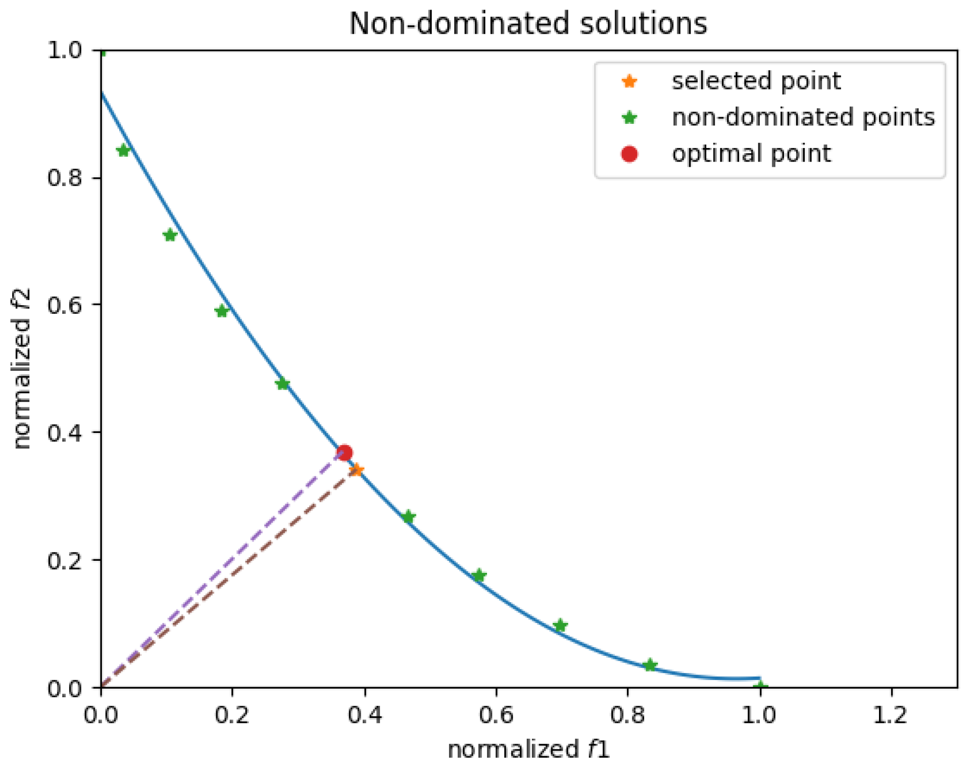
Most of the multi-objective methods tend to seek the optimal Pareto front, then select a single solution among the non-dominated solutions based on some criterion. Although finding the Pareto front could work in parallel, a complete front is required to find the compromise point. See Figure 1. We optimize over the criterion directly, which could find the solution more satisfied with the criterion and avoid looking for the Pareto front.

The “criterion” here is to minimize the Euclidean distance between non-dominated solution and the Utopian point. The Utopian point is the infeasible solution with each entry corresponds to the objective of a single-objective optimization problem [33]. For example, the objective of single-objective optimization $min$ $f1$ is the $f{1}_{min}$, while the objective of $min$ $f2$ is the $f{2}_{min}$. The Utopian point could be ($f{1}_{min}$,$f{2}_{min}$).

To optimize the criterion, the objective could be formed using the following formula.

$$minF=\sqrt{{F_1^{\prime }}^2+{F_2^{\prime }}^2}$$

(11)

where $F_1^{\prime }$, $F_2^{\prime }$ are the normalized objective of $F_1$ and $F_2$. Please note that minimize F is equivalent to minimize ${F_1^{\prime }}^2+{F_2^{\prime }}^2$, which is easier to be optimized. We regard F as MOUC cost.

3. Methodology

We propose a method based on the margin price (MP) in connected subsystems. A system-level operator collects margin price of subsystems. Please note that the margin price is calculated based on (11), which measures the sensitivity to change of the MOUC cost. The basic hypothesis is that for given subsystems, in any time intervals, the total MOUC cost would be decreased, if a little part of load is transferred from high margin price subsystem to the other. Please note that the margin price here is the MOUC cost of the next kWh of energy. During iteration, the system-level operator determines the optimal tie-line power flow and the generation of each subsystem based on MP, load balance constraint and tie-line constraint. Then, the subsystem updates their MP based on the generation. The new MP is uploaded to the system-level operator, and the tie-line power flow is updated again. The process continues until the stop criterion is met. The optimal solution is obtained when the difference of margin price between subsystems near zero. The proposed methodology for MOUC is shown below.

Step 1:

Initialize tie-line based on the total capability and local load in each subsystem.

Step 2:

Update virtual load in each subsystem based on tie-line.

Step 3:

Solve local MOUC problem in each subsystem and calculate MP.

Step 4:

Update tie-line based on MP and local load in subsystems.

Step 5:

If the stop criterion is met, the algorithm is terminated and the UC schedule is returned, otherwise, return to Step 3.

3.1. Initialize Tie-Line

A good initialization strategy of tie-line could lead to an improved result when performing the following procedures. The initialization strategy follows rules.

• The tie-line constraint (10) and system constraints should be met. To ensure the UC problems in subsystems are still feasible, the increase of generation in subsystem should meet constraint (5), which is denoted as $R{C}_{j,t}$ for subsystem j in (17).
• The total generation level in any pairs of subsystems depends on the total capability in each subsystem.

  $$\frac{{\mathrm{Capability}}_{\mathrm{A}}}{{\mathrm{Capability}}_{\mathrm{B}}}=\frac{Generatio{n}_{\mathrm{A}}}{Generatio{n}_{\mathrm{B}}}$$

  (12)
  The priority of these conditions is 1, 2.

The initialized tie-line could be obtained by solving the following problem.

$$\begin{array}{c}min\sum _t\sum _j{\left(\left(D_{j,t}+\sum _i{p}_{j,i,t}^{tie}\right)-D_{i,t}^{init}\right)}^2\hfill \end{array}$$

(13)

$$\begin{array}{cc}\hfill s.t.& p_{i,i,t}^{tie}=0,i\in \{1,\dots ,M\},t\in \{1,\dots ,T\}\hfill \end{array}$$

(14)

$$\begin{array}{c}{p}_{i,j,t}^{tie}+p_{j,i,t}^{tie}=0,i,j\in \{1,\dots ,M\},t\in \{1,\dots ,T\}\hfill \end{array}$$

(15)

$$\begin{array}{c}|p_{i,j,t}^{tie}|\le P_{i,j}^{max},i,j\in \{1,\dots ,M\},t\in \{1,\dots ,T\}\hfill \end{array}$$

(16)

$$\begin{array}{c}\sum _j{p}_{j,i,t}^{tie}\le R{C}_{j,t},i,j\in \{1,\dots ,M\},t\in \{1,\dots ,T\}\hfill \end{array}$$

(17)

where $p_{i,j,t}^{tie}$ is the power flow of tie-line from subsystem i to subsystem j at time t, consequently, ${\sum }_i{p}_{j,i,t}^{tie}$ is the generation which will be added to the subsystem. $P_{i,j}^{max}$ is the tie-line limit, if there is no tie-line between subsystem i and j, $P_{i,j}^{tie}$ could be set to 0. $D_{i,t}^{init}$ is constant calculated based on rule 2, which stands for the recommended load in subsystem i during time interval t.

Solving (13) can be easy as there is no time-dependent constraint and all variables $p_{j,i,t}^{tie}$ are continuous. Hence the initialized tie-line could be obtained by satisfying the recommended load as well as system constraints.

3.2. Update Virtual Load

The virtual load of subsystem is not the real load in the subsystem, but virtual load with consideration of the tie-line. The sum of virtual loads in all subsystems is still equal to the sum of real loads. The virtual load is updated based on the actual local load and tie-line.

$$V{L}_{i,t}=D_{i,t}+\sum _j{p}_{i,j,t}^{tie},i,j\in \{1,\dots ,M\},t\in \{1,\dots ,T\}$$

(18)

$V{L}_{i,t}$ is the virtual load in area i during time interval t. During the iteration process, we calculate the virtual load by (18), then, solve local MOUC with consideration of constraints in Section 2. The load demand in (4) is modified to virtual load to see the consequence of updated tie-line.

3.3. Calculate local MOUC

Local MOUC problems are solved using the branch and bound method, by solving (11) respects to constraints (4)–(9), and the load balance is updated as discussed above. Please note that solving local MOUC do not require additional information other than power flow of tie-line.

After solving the local MOUC problem for each subsystem, $M{P}_{i,t}$ should be by taking the derivative with respect to local load.

$${MP}_{i,t}=\frac{\partial F^{\prime }}{\partial V{L}_{i,t}},i\in \{1,\dots ,M\},t\in \{1,\dots ,T\}$$

(19)

As there is no closed form of $V{L}_{i,t}$ in (11), (19) could not be solved directly. So we apply Algorithm 1 to get $M{P}_{i,t}$.

Algorithm 1 Calculate multi-objective margin price in subsystem i

j is the index of unit in subsystem i $p_{j,t}$ is the scheduled output of unit j at time t $penalty=$ 100,000 initialize $gap>0$  1: for each $t\in \{1,\dots ,T\}$ do  2:   for each $j\in \{1,\dots ,N\}$ do  3:    if $p_{max}^j-p_{j,t}\le gap$ then  4:      $mp{u}_{j,t}=penalty$  5:    else  6:      $mp{u}_{j,t}=\frac{\partial F^{\prime }}{\partial p_{j,t}}$  7:    end if  8:   end for  9: $M{P}_{i,t}=min(mp{u}_{j,t}),j\in \{1,\dots ,N\}$ 10: end for 11: return$M{P}_i$

3.4. Update Tie-Line Power Flow

The tie-line power flow is updated based on the hypothesis that for any time intervals, if a little part of load is transferred from high $MP$ area to the other, the total MOUC cost in the whole system could be decreased, and the amount of change signifies the step size with direction defined by the difference between subsystems. The rules of updating tie-line power flow are summarized as follows.

• For any given time interval, the change of tie-line should decrease the total MOUC cost in the whole system. As the $MP$ has been calculated in the previous step, the subsystem with high $MP$ should generate less, and tie-line power flow could be updated as follows.

  $$\begin{array}{cc}\hfill & min\sum _t\sum _i\left({MP}_{i,t}\left(\sum _j{x}_{i,j,t}\right)\right)\hfill \end{array}$$

  (20)

  $$\begin{array}{c}\hfill s.t.\end{array}$$

  (21)

  $$\begin{array}{c}{x}_{i,i,t}=0,i\in \{1,\dots ,M\},t\in \{1,\dots ,T\}\hfill \end{array}$$

  (22)

  $$\begin{array}{c}{x}_{i,j,t}+x_{j,i,t}=0,i,j\in \{1,\dots ,M\},t\in \{1,\dots ,T\}\hfill \end{array}$$

  (23)

  $$\begin{array}{c}|x_{i,j,t}|\le P_{i,j}^{max},i,j\in \{1,\dots ,M\},t\in \{1,\dots ,T\}\hfill \end{array}$$

  (24)

  $$\begin{array}{c}|\sum _j{x}_{j,i,t}|\le Ste{p}_{i,t},i,j\in \{1,\dots ,M\},t\in \{1,\dots ,T\}\hfill \end{array}$$

  (25)

  $x_{i,j,t}$ is the step change which should be added to $p_{i,j,t}^{tie}$.

  $$P_{i,j,t}^{tie}=P_{i,j,t}^{tie}+x_{i,j,t},i,j\in \{1,\dots ,M\},t\in \{1,\dots ,T\}$$

  (26)
  $|{\sum }_j{x}_{j,i,t}|$ is the change of $V{L}_i$ at time t. We assumes that if the change of system load did not exceed $Ste{p}_{i,t}$, the $M{P}_{i,t}$ would be seen as constant. As a result, the objective of (20) represents the increase of total MOUC cost in the whole system.
• However, $Step$ must be chosen to update the tie-line power flow. $Step$ could neither be too big nor too small. A big $Step$ may cause the total MOUC cost to increase, because the direction is a decent direction only if the $Step$ is not too big in any time interval. Furthermore, a small $Step$ may lead to the total MOUC cost to be almost invariant, or will not encourage more units to be on. Here, $Step$ is chosen based on the following rules.

  (a)

  The $Ste{p}_t$ would be big, if the difference of margin price between the two subsystems is significant.

  (b)

  The $Ste{p}_t$ shall not only meet the tie-line constraint, but also ensure that it does not exceed a certain percentage of the local load of the two subsystems to which tie-line is connected.

  $$0\le Ste{p}_t\le \delta \times D_t$$

  (27)

  $\delta$ represents the percentage of load allowed to be changed.

  (c)

  The feasibility of UC problems related with subsystems should be guaranteed. The direct solution here is based on the observation that if system reserve constraint (5) is satisfied, then by modifying the output of units, it is easy to satisfy the demand constraint (4) [35].

  The algorithm of choosing the $Step$ could be stated as follows.

Algorithm 2 Find the $Step$ for subsystem i at time t

Input: system index i and time t get the UC schedule during last iteration $P_{max}={\sum }_k{P}_{k,max}$, where k is the index of unit in subsystem i  1: for each $j\in \{1,\cdots ,M\}$ do  2:   if $j=i$ then  3:    $step{s}_j=0$  4:   else  5:    $step{s}_j=\frac{|{MP}_{i,t}-{MP}_{j,t}|}{max({MP}_{i,t},{MP}_{j,t})}·\delta ·min(D_{i,t},D_{j,t})$  6:   end if  7: end for  8: $ste{p}_{i,t}=max(step{s}_j),j\in \{1\dots M\}$  9: if$P_{max}\le D_{i,t}+R_{i,t}+ste{p}_{i,t}$then 10:    $ste{p}_{i,t}=D_{i,t}+R_{i,t}-Pmax$ 11: end if 12: return$Ste{p}_{i,t}$

The parameter $\delta$ varies from system to system. If the $MP$ in subsystem i is quite low, the generation of subsystem i would increase by $Step$. As the iteration moving on, the increased generation will encourage more units in subsystem i to be on, and $P_{max}$ in line 10 of the Algorithm above will be bigger to encourage more generation(if the $MP$ in the subsystem is still low).

3.5. Stop Criterion

The stop criterion is of great interest that we should ensure either the optimality as well as convergence. A natural idea is that the difference of $MP$ between any pairs of subsystems attached with a tie-line is the criterion of convergence because we are taking the difference of $MP$ as an iterative basis, but the difference of $MP$ between subsystems may never be zero as there are other constraints like system reserve constraint (5) and tie-line constraint (10). Therefore, the stop criterion could be formed as the following rules.

• If $|{MP}_{i,t}-{MP}_{j,t}|<\theta ,(i\ne j)$ is met at all time intervals and $P_{i,j}^{max}\ne 0$ (there exists a tie-line between subsystem i and j), or the change MOUC cost is almost invariant, the iteration process is terminated.
• If the tie-line power flow has reached its limit or the maximum number of iterations been reached, stops updating the tie-line.
• When the subsystem spinning reserve has been reached and the $MP$ of that subsystem is still low, which means, if the tie-line encourages the generation of that subsystem to be decreased, the total MOUC cost would increase, but the generation should not be increased. So the attached tie-line should not be updated anymore.

Theorem 1.

There exits an equilibrium so the iteration process could be terminated.

Proof. 

We focus on the situation where rules 2 and 3 have not been met. The $MP$ of subsystem is defined as the first-order derivative of one of the units in the subsystem. Assumes the $MP$ of unit i is the lowest. So, the $MP$ for the subsystem at time t could be written as derivative with respect to the unit output that belongs to the subsystem.

$$MP=\frac{\partial F^{\prime }}{\partial p_{i,t}}=2F_1^{\prime }\frac{\partial F_1^{\prime }}{\partial p_{i,t}}+2F_2^{\prime }\frac{\partial F_2^{\prime }}{\partial p_{i,t}}$$

(28)

Please note that the $MP$ at time t can be influenced by not only $p_{i,t}$, but also the output of other units at any time intervals. If the system load is increased by $Step$, the generation of some units (especially the one with lowest $MP$) would be increased and vice versus. So we look at the influence on $MP$ when the output of some units have changed.

$$\frac{\partial MP}{\partial p_{i,t}}=2{\left(\frac{\partial F_1^{\prime }}{\partial p_{i,t}}\right)}^2+2{\left(\frac{\partial F_2^{\prime }}{\partial p_{i,t}}\right)}^2+2F_1^{\prime }\frac{{\partial }^2{F}_1^{\prime }}{\partial p_{i,t}^2}+2F_2^{\prime }\frac{{\partial }^2{F}_2^{\prime }}{\partial p_{i,t}^2}$$

(29)

Each term in (29) is only influenced by parameters of unit i. For any units, the coeffcients of fuel cost function (1) are always positive, which means the first and third term in (29) are positive. As for the first and second order derivative of (3), we refer to [36] that these derivatives are always positive when $p_{i,t}\in \{P_{i,min},P_{i,max}\}$.

Hence, for all units, (29) has always been positive when $p_{i,t}\in \{P_{i,min},P_{i,max}\}$. If the output of any units in that subsystem is increased, the $MP$ of the subsystem must be increased and vice versus. As the iteration process moving on, the $MP$ between pairs of subsystem could be closing to each other.

Please note that the proof above based on the unit with lowest margin price is not changed with the iteration process going on. If the margin unit has been changed, the proof could also make sense:

• If the margin unit in the last iteration step has been scheduled to generate at its full capacity, the margin unit will be changed, and there will be a gap of the $MP$. The (29) could also be positive because the if the generation of new margin unit is increased, $MP$ is increased, and if the $VL$ of the system is decreased, margin unit would be switched to that in the last iteration step, the $MP$ is decreased.
• If the margin unit has been changed and the margin unit in the last iteration step has not reached its generation limit, the (29) will not be consistent, but it is still positive.

Furthermore, for any tie-line updated based on rule 1, the convergence could be guaranteed. □

Theorem 2.

The iterative process converges to the local optimum.

Proof. 

The MOUC cost of the whole system could be written as a function of tie-line.

$$\begin{array}{c}min{F}^{\prime }=\sum _t\sum _i{f}_i^{\prime }\left(D_{i,t}+\sum _j{p}_{i,j,t}^{tie}\right)\hfill \end{array}$$

(30)

$$\begin{array}{c}\hfill s.t.\end{array}$$

(31)

$$\begin{array}{c}{p}_{i,j,t}^{tie}=-p_{j,i,t}^{tie},i,j\in \{1,...,M\},t\in \{1,...,T\}\hfill \end{array}$$

(32)

$$\begin{array}{c}{p}_{i,i,t}^{tie}=0,i\in \{1,...,M\},t\in \{1,...,T\}\hfill \end{array}$$

(33)

$$\begin{array}{c}|p_{i,j,t}^{tie}|\le P_{i,j,t}^{max},i,j\in \{1,...,M\},t\in \{1,...,T\}\hfill \end{array}$$

(34)

$f_i^{\prime }(x)$ is the function of MOUC cost for subsystem i. Adding the Lagrange multiplier, using the constraint (33), and setting derivative with respect to $p_{i,j,t}^{tie}$ equal to zero (if there exists tie-line between sybsystem i and j), we get:

$$\begin{array}{c}\hfill \frac{\partial f_i^{\prime }\left(D_{i,t}+{\sum }_k{p}_{i,k,t}^{tie}\right)}{\partial p_{i,j,t}^{tie}}-\frac{\partial f_j^{\prime }\left(D_{j,t}+{\sum }_k{p}_{j,k,t}^{tie}\right)}{\partial p_{i,j,t}^{tie}}\\ \hfill ={\lambda }_{i,j}^{max}-{\lambda }_{i,j}^{min}+{\lambda }_{j,i}^{max}-{\lambda }_{j,i}^{min}\end{array}$$

(35)

where ${\lambda }_{i,j}^{max}$ is the Lagrangian multiplier of inequality constraint $p_{i,j,t}^{tie}\le P_{i,j,t}^{max}$, and ${\lambda }_{i,j}^{min}$ is for $p_{i,j,t}^{tie}\ge P_{i,j,t}^{min}$. When rule 1 is met and rule 2, 3 have not been met, constraint (34) is satisfied, $\lambda$ in (35) is zero. Then, for subsystem i, j, the derivative of MOUC cost with respect to attached tie-line power flow, or, $MP$ of subsystems, are equal to each other. which is the same solution as our algorithm. If $\lambda \ne 0$, the boundary of constraint (34) has been met, then we still get the same solution as our algorithm considering rule 2. Furthermore, we have considered the feasibility of local MOUC. □

Please note that units parameters in each subsystem are not required to be uploaded. For each subsystem, only local $MP$ and the cost for each objective (fuel cost and gas emission in this article) are required, which protects the privacy of generating companies.

4. Numerical Examples

The algorithm was coded in JAVA, and had been performed on a workstation with Intel i5-6600K processor and 16GB of RAM under Windows operating system. A test case was conducted to emphasize the robustness of the algorithm, which includes two subsystems and the result is compared with the weighted-sum [37] and NBI [38,39].

The tie-line limit in (10) is set to 100 MW, and $\delta$ in Algorithm 2 varies from cases.

4.1. 46 Units Test

A 46 units case is applied to illustrate the performance of the proposed algorithm. The whole system is divided into two subsystems, one has 10 units and the other has 36 units. The 10 units fuel and gas parameters are referenced from [40], and 36 units thermal parameters are from [41]. The gas efficients for 36 units are referenced from 10 units case, with high cost units are assigned bigger emission function. The parameters of units is shown in the Appendix A.

The initial condition time (ICT) in the appendix corresponds to the operating status before time 1. For example, initial condition hour ‘−3’ means the unit had been turned off for 3 h before time 1, and 4 means the unit had been turned on for 4 h before time 1. The threshold $\theta$ in Section 3.5 is set to 10$/t and $\delta$ in Algorithm 2 is set to 0.02.

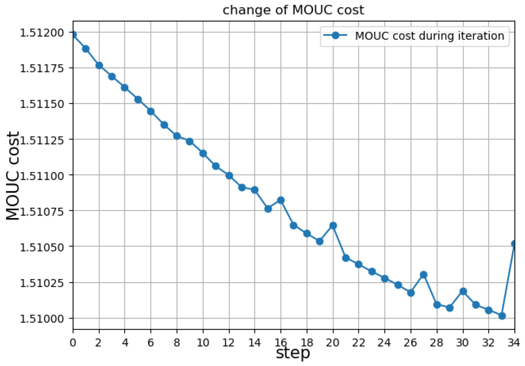
The initialized tie-line power flow and that during iteration process can be seen in Figure 2. During the iteration process, the tie-line had been approaching its limit at some time intervals, and the margin price had been closed to each other as shown in Figure 3. The gray area in Figure 3 represents the difference of the margin price between subsystems, and the area becomes smaller with the iteration going on. The iteration process is terminated due to rule 1 in Section 3.5. The total MOUC cost is decreasing during iteration, which had been shown in Figure 4.

The MOUC cost is decreasing in the first 30 steps, and then converges to about 1.51. The thermal cost and the emission during the iteration process have been shown in Figure 5.

4.2. Comparing with Other Methods

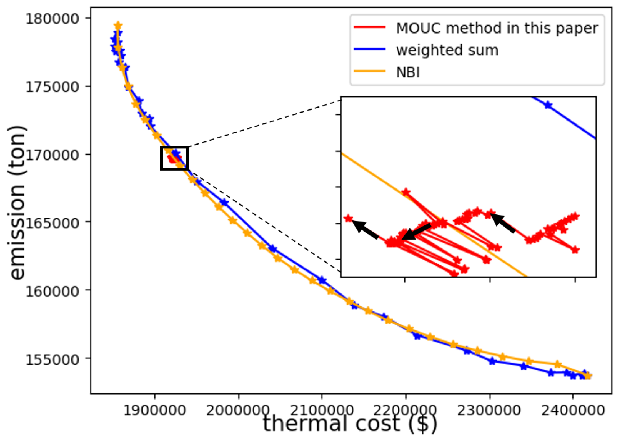
One important contribution of this paper is that the strategy of finding the compromise solution is directly optimized in the objective function in (11), which avoids looking for other non-dominated solutions as described in Section 2.3. The MOUC solution in this paper is compared with other two MOUC methods namely weighted-sum [37] and NBI [38,39]. In addition, the results and computation times have been shown in Figure 5 and

Table 1. Computation times.

	Weighted Sum	NBI	MOUC Method in This Paper
Time (S)	1775	3647	1294

respectively.

In conventional methods, the Pareto front is calculated by weighted-sum and NBI, then the best solution with respect to (11) is selected among the Pareto front. Hence, in order to find a better compromise solution, a denser Pareto front is required. In Figure 5, for weighted-sum and NBI, we use each algorithm to calculate 30 non-dominated solutions to obtain the Pareto front. The initialization strategy of this paper can make the solution of our method better than the result of weighted-sum, but not as good as that of NBI. However, as the iterative process progresses, our method ultimately finds solutions that are better than the NBI method. Besides, in the proposed problem formulation, the UC problem only needs to be solved for one time, hence, the efficiency outperforms weighted sum and NBI as seen in Table 1.

5. Conclusions

This paper proposes a novel MOUC model and a decomposition coordination method to solve it considering tie-line constraint. To minimize the production cost and emission, the multi-objective problem is transformed into a single objective, instead of generating a complete Pareto front or assigning weight to each objective, we minimize the Euclidean distance to the Utopian point, as a result, a better solution which is more satisfied with the proposed criterion could be found.

Then, we calculate the revised problem by an iteration process. During the iteration process, the margin price in connected subsystems is regarded as the coordinator to update tie-line, and we realize exact step control by considering the margin price, total load, etc. Each subsystem is solved separately and locally by the branch and bound method. Test cases indicate that our method could obtain an improved result than weighted-sum and NBI. Besides, solving local MOUC problem avoids the need for uploading units parameters, which protects the data privacy of generating companies.

For any given two subsystems, if the subsystem with a high margin price generates less while the other generates more, the total cost would be decreased. However, the step size is chosen by a subjective approach, and we have not found the optimal step. In addition, the solution is very sensitive to the initialization strategy, maybe we could solve MOUC based on a parallel way, with different initialized tie-line. Furthermore, we could apply DNN [42] to find the underlying relationship among units, load, tie-line as well as step size in the future.

References

- Frangioni, A.; Gentile, C. Solving nonlinear single-unit commitment problems with ramping constraints. Oper. Res. 2006, 54, 767–775. [Google Scholar] [CrossRef]
- Guan, X.; Zhai, Q.; Papalexopoulos, A. Optimization based methods for unit commitment: Lagrangian relaxation versus general mixed integer programming. In Proceedings of the Power Engineering Society General Meeting, Toronto, ON, Canada, 13–17 July 2003; Volume 2, pp. 1095–1100. [Google Scholar]
- Johnson, R.; Happ, H.; Wright, W. Large scale hydro-thermal unit commitment-method and results. IEEE Trans. Power Appar. Syst. 1971, PAS-90, 1373–1384. [Google Scholar] [CrossRef]
- Bertsekas, D.P.; Bertsekas, D.P.; Bertsekas, D.P.; Bertsekas, D.P. Dynamic Programming and Optimal Control; Athena Scientific: Belmont, MA, USA, 1995; Volume 1. [Google Scholar]
- Zhai, Q.; Guan, X.; Cui, J. Unit commitment with identical units successive subproblem solving method based on Lagrangian relaxation. IEEE Trans. Power Syst. 2002, 17, 1250–1257. [Google Scholar] [CrossRef] [Green Version]
- Morales-España, G.; Latorre, J.M.; Ramos, A. Tight and compact MILP formulation for the thermal unit commitment problem. IEEE Trans. Power Syst. 2013, 28, 4897–4908. [Google Scholar] [CrossRef]
- Alemany, J.; Magnago, F.; Moitre, D.; Pinto, H. Symmetry issues in mixed integer programming based Unit Commitment. Int. J. Electr. Power Energy Syst. 2014, 54, 86–90. [Google Scholar] [CrossRef]
- Lei, X.; Guan, X.; Zhai, Q. Constructing Valid Inequalities by Analytical Feasibility Conditions on Unit Commitment with Transmission Constraints. IEEE Trans. Power Syst. 2016, 31, 3484–3494. [Google Scholar] [CrossRef]
- Pan, K.; Guan, Y.; Watson, J.P.; Wang, J. Strengthened MILP Formulation for Certain Gas Turbine Unit Commitment Problems. IEEE Trans. Power Syst. 2016, 31, 1440–1448. [Google Scholar] [CrossRef]
- Todosijevic, R.; Mladenovic, M.; Hanafi, S.; Mladenovic, N.; Crevits, I. Adaptive general variable neighborhood search heuristics for solving the unit commitment problem. Int. J. Electr. Power Energy Syst. 2016, 78, 873–883. [Google Scholar] [CrossRef]
- Wang, C.; Fu, Y. Fully parallel stochastic security-constrained unit commitment. IEEE Trans. Power Syst. 2016, 31, 3561–3571. [Google Scholar] [CrossRef]
- Trivedi, A.; Srinivasan, D.; Pal, K.; Saha, C.; Reindl, T. Enhanced multiobjective evolutionary algorithm based on decomposition for solving the unit commitment problem. IEEE Trans. Ind. Inform. 2015, 11, 1346–1357. [Google Scholar] [CrossRef]
- Nemati, M.; Braun, M.; Tenbohlen, S. Optimization of unit commitment and economic dispatch in microgrids based on genetic algorithm and mixed integer linear programming. Appl. Energy 2018, 210, 944–963. [Google Scholar] [CrossRef]
- Shukla, A.; Singh, S. Advanced three-stage pseudo-inspired weight-improved crazy particle swarm optimization for unit commitment problem. Energy 2016, 96, 23–36. [Google Scholar] [CrossRef]
- Trivedi, A.; Srinivasan, D.; Biswas, S.; Reindl, T. A genetic algorithm–differential evolution based hybrid framework: case study on unit commitment scheduling problem. Inf. Sci. 2016, 354, 275–300. [Google Scholar] [CrossRef]
- Dhillon, J.; Parti, S.; Kothari, D. Stochastic economic emission load dispatch. Electric Power Syst. Res. 1993, 26, 179–186. [Google Scholar] [CrossRef]
- Yokoyama, R.; Bae, S.; Morita, T.; Sasaki, H. Multiobjective optimal generation dispatch based on probability security criteria. IEEE Trans. Power Syst. 1988, 3, 317–324. [Google Scholar] [CrossRef]
- Abido, M.A. Environmental/economic power dispatch using multiobjective evolutionary algorithms. IEEE Trans. Power Syst. 2003, 18, 1529–1537. [Google Scholar] [CrossRef]
- Wang, L.; Singh, C. Environmental/economic power dispatch using a fuzzified multi-objective particle swarm optimization algorithm. Electr. Power Syst. Res. 2007, 77, 1654–1664. [Google Scholar] [CrossRef]
- Cai, J.; Ma, X.; Li, Q.; Li, L.; Peng, H. A multi-objective chaotic ant swarm optimization for environmental/ economic dispatch. Int. J. Electr. Power Energy Syst. 2010, 32, 337–344. [Google Scholar] [CrossRef]
- Norouzi, M.R.; Ahmadi, A.; Nezhad, A.E.; Ghaedi, A. Mixed integer programming of multi-objective security-constrained hydro/thermal unit commitment. Renew. Sustain. Energy Rev. 2014, 29, 911–923. [Google Scholar] [CrossRef]
- Li, Y.F.; Pedroni, N.; Zio, E. A memetic evolutionary multi-objective optimization method for environmental power unit commitment. IEEE Trans. Power Syst. 2013, 28, 2660–2669. [Google Scholar] [CrossRef]
- Kockar, I. Unit commitment for combined pool/bilateral markets with emissions trading. In Proceedings of the 2008 IEEE Power and Energy Society General Meeting—Conversion and Delivery of Electrical Energy in the 21st Century, Pittsburgh, PA, USA, 20–24 July 2008; pp. 1–9. [Google Scholar]
- Ma, H.; Shahidehpour, S. Transmission-constrained unit commitment based on Benders decomposition. Int. J. Electr. Power Energy Syst. 1998, 20, 287–294. [Google Scholar] [CrossRef]
- Maheswari, S.; Vijayalakshmi, C. A lagrangian decomposition model for unit commitment problem. Int. J. Comput. Appl. 2012, 43, 21–25. [Google Scholar] [CrossRef]
- Fu, Y.; Shahidehpour, M.; Li, Z. Long-term security-constrained unit commitment: Hybrid Dantzig-Wolfe decomposition and subgradient approach. IEEE Trans. Power Syst. 2005, 20, 2093–2106. [Google Scholar] [CrossRef]
- Li, M.Y.; Luh, P.B. A decentralized framework of unit commitment for future power markets. In Proceedings of the 2013 IEEE Power and Energy Society General Meeting, Vancouver, BC, Canada, 21–25 July 2013; pp. 1–5. [Google Scholar]
- Nedic, A. Asynchronous broadcast-based convex optimization over a network. IEEE Trans. Autom. Control 2011, 56, 1337–1351. [Google Scholar] [CrossRef]
- Trivedi, A.; Srinivasan, D.; Pal, K.; Reindl, T. A multiobjective evolutionary algorithm based on decomposition for unit commitment problem with significant wind penetration. In Proceedings of the 2016 IEEE Congress on Evolutionary Computation (CEC), Vancouver, BC, Canada, 24–29 July 2016; pp. 3939–3946. [Google Scholar]
- Younes, M.; Khodja, F.; Kherfane, R.L. Multi-objective economic emission dispatch solution using hybrid FFA (firefly algorithm) and considering wind power penetration. Energy 2014, 67, 595–606. [Google Scholar] [CrossRef]
- Albers, S.; Eilts, S.; Even-Dar, E.; Mansour, Y.; Roditty, L. On Nash equilibria for a network creation game. ACM Trans. Econ. Comput. 2014, 2, 89–98. [Google Scholar] [CrossRef]
- Carrión, M.; Arroyo, J.M. A computationally efficient mixed-integer linear formulation for the thermal unit commitment problem. IEEE Trans. Power Syst. 2006, 21, 1371–1378. [Google Scholar] [CrossRef]
- Qi, Y.; Zhang, Q.; Ma, X.; Quan, Y.; Miao, Q. Utopian point based decomposition for multi-objective optimization problems with complicated Pareto fronts. Appl. Soft Comput. 2017, 61, 844–859. [Google Scholar] [CrossRef]
- Cao, J.; Yan, Z.; He, G. Application of Multi-Objective Human Learning Optimization Method to Solve AC/DC Multi-Objective Optimal Power Flow Problem. Int. J. Emerg. Electr. Power Syst. 2016, 17, 327–337. [Google Scholar] [CrossRef]
- Virmani, S.; Adrian, E.C.; Imhof, K.; Mukherjee, S. Implementation of a Lagrangian relaxation based unit commitment problem. IEEE Trans. Power Syst. 1989, 4, 1373–1380. [Google Scholar] [CrossRef]
- Gent, M.; Lamont, J.W. Minimum-emission dispatch. IEEE Trans. Power Appar. Syst. 1971, PAS-90, 2650–2660. [Google Scholar] [CrossRef]
- Dhillon, J.; Parti, S.; Kothari, D. Fuzzy decision-making in stochastic multiobjective short-term hydrothermal scheduling. IEE Proc. Gener. Transm. Distrib. 2002, 149, 191–200. [Google Scholar] [CrossRef]
- Wang, H.; Xu, X.; Zheng, Y. Multi-Objective Optimization of Security Constrained Unit Commitment Model and Solution Considering Flexible Load. Power Syst. Technol. 2017, 41, 1904–1912. [Google Scholar]
- Ahmadi, A.; Moghimi, H.; Nezhad, A.E.; Agelidis, V.G.; Sharaf, A.M. Multi-objective economic emission dispatch considering combined heat and power by normal boundary intersection method. Electr. Power Syst. Res. 2015, 129, 32–43. [Google Scholar] [CrossRef]
- Zhang, X.-H.; Zhao, J.-Q. Unit commitment by enhanced adaptive Lagrangian relaxation. Proc. CSEE 2010, 30, 71–76. [Google Scholar]
- Ma, H.; Shahidehpour, S. Unit commitment with transmission security and voltage constraints. IEEE Trans. Power Syst. 1999, 14, 757–764. [Google Scholar] [CrossRef]
- Cireşan, D.; Meier, U.; Masci, J.; Schmidhuber, J. Multi-column deep neural network for traffic sign classification. Neural Netw. 2012, 32, 333–338. [Google Scholar] [CrossRef] [PubMed] [Green Version]
Figure 1.
If we want to improve the compromise solution, a denser Pareto front is required [34], so we could select a better solution among the front. However, optimizing the criterion directly could find a better compromise solution and avoids looking for other non-dominated solutions.
Figure 2.
Tie-line during iteration process.
Figure 3.
Margin price during iteration process.
Figure 4.
MOUC cost during iteration process.