An Investigation on the Forced Convection of Al₂O₃-water Nanofluid Laminar Flow in a Microchannel Under Interval Uncertainties

Abstract

Nanofluids are regarded as an effective cooling medium with tremendous potential in heat transfer enhancement. In reality, nanofluids in microchannels are at the mercy of uncertainties unavoidably due to manufacturing error, dispersion of physical properties, and inconstant operating conditions. To obtain a deeper understanding of forced convection of nanofluids in microchannels, uncertainties are suggested to be considered. This paper studies numerically the uncertain forced convection of Al₂O₃-water nanofluid laminar flow in a grooved microchannel. Uncertainties in material properties and geometrical parameter are considered. The uncertainties are represented by interval variables. By employing Chebyshev polynomial approximation, interval method (IM) is presented to estimate the uncertain thermal performance and flow behavior of the forced convection problem. The validation of the accuracy and effectiveness of IM are demonstrated by a comparison with the scanning method (SM). The variation of temperature, velocity, and Nusselt number are obtained under different interval uncertainties. The results show that the uncertainties have remarkable influences on the simulated thermal performance and flow behavior.

1. Introduction

In the traditional numerical investigations on the forced convection problem, the parameters that affect the thermal performance and flow behavior are treated as deterministic values. However, for complicated convection heat transfer problem in the real world, uncertainties exist naturally. To obtain a deeper understanding of the forced convection problem of nanofluids in microchannels, uncertainties are suggested to be considered.

In 2000, Xuan et al. [1] pointed out that nanofluids had tremendous potential in heat transfer enhancement. Then they investigated the transport and thermal performances of nanofluids and proposed two fitting methods for heat transfer correlations. Maiga et al. [2] investigated the laminar convection heat transfer performance of nanofluids in two different types of passages. Comparisons were carried out between Al₂O₃-water and Al₂O₃-Ethylene Glycol. As concluded in this study, nanofluids could improve thermal performance and this effect was strengthened with the increase in particle concentration. The latter had better thermal performance than the former. He et al. [3] experimentally studied the thermal behavior of TiO₂ nanofluids in vertical tubes, covering laminar, turbulence, and transition states. It was pointed out that nanoparticles increased thermal conductivity and the beneficial effect was more significant at a larger particle concentration and a smaller particle size. An experimental system of a circular channel with nanofluids flow was constructed by Heris et al. [4]. They studied the heat transfer performance under isothermal wall temperature conditions. The experimental results were obviously higher than the prediction results by single phase heat transfer correlation. Nada et al. [5] performed numerical investigations on the natural convection heat transfer of various water-based nanofluids in horizontal annular tubes, and TiO₂, Ag, Cu, and Al₂O₃ nanoparticles were considered. They suggested that the heat transfer was significantly influenced by the Rayleigh number and coefficient of thermal conduction of nanoparticles. Jung et al. [6] experimentally studied the heat transfer and flow behavior of Al₂O₃-water nanofluids in rectangular microchannels. Wherein, the diameter of nanoparticles was 170 nm. They found that, under laminar condition, the adoption of 1.8% nanofluids improved the heat transfer coefficient by 32% compared with water, meanwhile, no obvious resistance loss was produced. Hwang et al. [7] measured the thermal conductivity and pressure drop of Al₂O₃-water nanofluids in uniformly heated tubes. They found that the friction data were in accord with prediction results of the Darcy equation, while the heat transfer enhancement was not in good agreement with the Shah equation. Duangthongsuk et al. [8,9] reported an experimental study on turbulence heat transfer of TiO₂-water nanofluids in a double-tube counterflow heat exchanger. In their study, the solid volume fraction is 0.2–2%. The results showed that the heat transfer could be improved by 6–11% using nanofluids, and a larger friction was also produced. Then they presented correlations of the Nusselt number and the friction factor based on experimental results. Akbari et al. [10] established microchannels with ribs and carried out a numerical investigation on laminar (Re = 10–100) heat transfer behavior of Al₂O₃-water nanofluids of which the maximum volume fraction was 0.04%. Effects of the ribs height and position, nanoparticle concentration, and Re on thermal-hydraulic performance were discussed. It was shown that the increase of rib height and nanoparticle concentration were beneficial to the heat transfer performance. Sekrani et al. [11] studied the flow and heat transfer of nanofluids in horizontal passages using direct numerical simulation. They found that, compared with the single-phase model, the two-phase model provided higher prediction accuracy. Moreover, effects of the nanoparticle type and diameter were also explored and empirical correlations of the Nusselt number and coefficient of friction were proposed. Hussain et al. [12] proposed a mathematical model to analyze the thermal performance and flow behavior of nanofluids on porous media plate. It was suggested that the increase of porous media permeability, nanofluids viscosity, and velocity slip parameter could reduce the thermal boundary layer and improve heat transfer performance. Fetecau et al. [13] obtained the heat transfer and flow behavior of fractional nanofluids in isothermal vertical tubes under heat radiation. Temperature, velocity, Nusselt number, and friction factor were provided, and a comparison was conducted between fractional ordinary nanofluids. Zhao et al. [14] predicted the viscosity of different types of nanofluids. Experimental results of Ethylene Glycol/water-based CuO, TiO₂, SiO₂, and SiC were used to train the neural network, and high prediction accuracy could be reached.

Valuable results concerning heat transfer and the flow of nanofluids have been obtained through deterministic analysis. However, the uncertainty is inevitable due to manufacturing errors, measurement errors, and variable working conditions, which will lead to uncertain thermal performance and flow behavior. For the purpose of taking uncertainties into account, the probabilistic numerical method [15], fuzzy theory [16], and interval method [17] have been developed. Monte Carlo simulation (MCS) [18] and polynomial chaos method [19,20], which belong to the probabilistic method are a valuable solution procedure that can handle the uncertainties. However, the uncertainties in the probabilistic method are treated as stochastic variables whose probability distribution function should be known in advance, which is tough work in reality. The fuzzy theory introduced by Zadeh [21] is an efficient method when uncertainty is considered. The uncertainties in the fuzzy theory are subject to the expert opinions, which should be determined beforehand. In the probabilistic method and the fuzzy theory, the information which is not easy to get about uncertainties is required. In some circumstances, assumptions of the probability distribution function are made when applying the above methods, which will lead to unexpected error and is unreliable. IM is such a method that can overcome the disadvantages of determining a large amount of information in advance in the above methods.

IM is widely employed to analyze the uncertainty problem. Only the bounds of uncertainties are required to determine the bounds of the interested properties. The advantage of IM is it is free of the probability distribution function of uncertainties. Pereira et al. [22] predicted the uncertain temperature of the transient heat conduction in a basin. To avoid overestimations, an element-by-element technique was proposed. Villacci and Vaccaro [23] employed interval mathematics to analyze the transient temperature tolerance in a power cable. The bounds of temperature were predicted, and the results were proved to be conservative in comparison with those obtained by MCS. Xue and Yang [24] investigated the uncertain response of a convection diffusion problem by employing IM based on the Taylor and Neumann expansion procedure. Wang et al. [17] proposed two variations of IM to estimate the bounds of temperature in heat convection-diffusion problems, and different types of uncertainties were taken into account. Then, in their latter work [25], they regarded the fuzzy parameters as interval variables and analyzed the fuzzy uncertainty propagation in a heat conduction problem.

IM has been widely used in uncertain thermodynamics, uncertain structure response [26,27,28], and uncertain rotor dynamics [29,30,31]. However, few papers about uncertain forced convection of nanofluids in microchannels have been published, which motivates this study. Based on the Chebyshev polynomial approximation, IM is proposed to analyze the uncertain thermal performance and flow behavior with uncertainties in material properties and geometric parameter. A comparison is made between IM and SM, which proves the effectiveness and accuracy of IM. Finally, the bounds of the temperature, velocity, and Nusselt number under different interval uncertainties are predicted.

2. Methodology

2.1. Phyical Model and Numerical Method

The schematic diagram of nanofluid flow in a grooved microchannel is shown in Figure 1. This two-dimensional model has a length of L = 500 μm and a height of H = 25 μm.

Table 1. The geometric parameters of the microchannel.

Notation	Description	Value
L1	Length of the entrance section	75 μm
L2	Length of the middle section	350 μm
L3	Length of the exit section	75 μm
δ	Depth of the grooves	10 μm
D	Length of the grooves	50 μm
W	Length of gap on each size of the grooved channel	75 μm

lists the detailed geometric parameters of the microchannel. The entrance section and the exit section are adiabatic. A condition of constant temperature T_h = 303 K is applied to the wall of the middle section. The nanofluid has a constant temperature of T_c = 293 K at x = 0 μm. Nonslip velocity boundary is considered on all the walls. The nanofluid is assumed to be fully developed at x = 0 μm. And the nanofluid exits the microchannel at atmospheric pressure.

To obtain the thermal performance and flow behavior of the forced convection problem, steady and incompressible flow is supposed. A single-phase model and constant physical property are adopted. Therefore, the governing equations of continuity, momentum and energy are

$$\frac{\partial u}{\partial x}+\frac{\partial v}{\partial y}=0$$

(1)

$$u\frac{\partial u}{\partial x}+v\frac{\partial u}{\partial y}=-\frac{1}{{\rho }_{nf}}\frac{\partial p}{\partial x}+\frac{{\mu }_{nf}}{{\rho }_{nf}}\left(\frac{{\partial }^{2}u}{\partial x^2}+\frac{{\partial }^{2}u}{\partial y^2}\right)$$

(2)

$$u\frac{\partial v}{\partial x}+v\frac{\partial v}{\partial y}=-\frac{1}{{\rho }_{nf}}\frac{\partial p}{\partial x}+\frac{{\mu }_{nf}}{{\rho }_{nf}}\left(\frac{{\partial }^{2}v}{\partial x^2}+\frac{{\partial }^{2}v}{\partial y^2}\right)$$

(3)

$$u\frac{\partial T}{\partial x}+v\frac{\partial T}{\partial y}={\alpha }_{nf}\left(\frac{{\partial }^{2}T}{\partial x^2}+\frac{{\partial }^{2}T}{\partial y^2}\right)$$

(4)

where u and v are the velocity along the x direction and y direction, respectively; p and T are the pressure and the temperature, respectively; and α and μ and ρ are the thermal diffusivities, the dynamic viscosity and the density, respectively.

Finite volume method combined with second-order upwind discretization scheme is utilized to solve all equations. Semi Implicit Method Pressure Linked Equation (SIMPLE) and pressure-velocity coupling method is employed in numerical calculation. As the residuals of the governing equations are less than 10⁻⁶, and the wall temperature and pressure drop residuals between adjacent iterative steps are less than 0.1%, the numerical calculation is considered to be convergent.

2.2. Phyical Properties of Nanofluid

The Al₂O₃-water nanofluid composed of base fluid (water) and Al₂O₃ are adopted in this study. The diameter of the nanoparticle is set to be 30 nm.

Table 2. Physical properties of water and Al₂O₃ nanoparticle (293 K).

Substance	k/W·m−1·K−1	Cp/J·kg−1·K−1	ρ/kg·m−3	μ/Pa·s
Al2O3	36.00	773.00	3880.00	-
Water	0.597	4182.00	998.20	9.93 × 10−4

lists the physical properties of water and nanoparticle. A single-phase model and constant physical property are adopted. The nanoparticle is assumed to be spherical and homogeneously suspended in water.

The models used to obtain the physical properties of nanofluid can be expressed as:

• Density model ρ:

  $${\rho }_{nf}=(1-\varphi ){\rho }_b+\varphi {\rho }_p$$

  (5)

  where the subscription nf, b and p denote the properties of nanofluid, water and Al₂O₃ nanoparticle, respectively; φ is the solid volume fraction.
• Specific heat model C_p [32]:

  $$C_{p_{nf}}=\frac{(1-\varphi )C_{p_b}{\rho }_b+\varphi C_{p_p}{\rho }_p}{{\rho }_{nf}}$$

  (6)
• Dynamic viscosity model μ [2]:

  $${\mu }_{nf}={\mu }_b(123{\varphi }^2+7.3\varphi +1)$$

  (7)
• Thermal conductivity model k [33]:

  $$k_{nf}=0.25\left[(3\varphi -1)k_p+(2-3\varphi )k_b+\sqrt{\Delta }\right]$$

  (8)

  where

  $$\Delta ={\left[(3\varphi -1)k_p+(2-3\varphi )k_b\right]}^2+8k_p{k}_b$$

  (9)

The dimensionless local Nusselt number (Nu) [34] is defined as

$$\mathrm{Nu}=-\frac{k_{nf}}{k_b}\left(\frac{\partial \theta }{\partial Y}\right)$$

(10)

where θ and Y are the dimensionless temperature and the y coordinate, respectively, and can be expressed as

$$\theta =\frac{T-T_c}{T_h-T_c}$$

(11)

$$Y=\frac{y}{H}$$

(12)

The average Nusselt number (Nu_m) of the middle section is defined by

$${\mathrm{Nu}}_m=\frac{1}{L_2}{\displaystyle {\int }_{L_1}^{L_1+L_2}\mathrm{Nu}(x)}dx$$

(13)

Besides, the Reynolds number can be expressed as

$$\mathrm{Re}=\frac{{\rho }_{nf}{u}_{c}H}{{\mu }_{nf}}$$

(14)

2.3. Uncertain Thermal Performace and Flow Behavior Prediction

Once the material properties of nanofluid and the boundary conditions are determined, the thermal performance and flow behavior can be obtained based on the physical model and numerical method presented in Section 2.2. A numerical calculation under determined parameters is called a deterministic calculation or a sample, which is widely utilized to study the thermal performance and flow behavior of forced convection problems by a series of deterministic calculations. As mentioned before, the forced convection problem is always at the mercy of uncertainties. Therefore, IM is employed to analyze the uncertain forced convection problem.

This section aims to build the surrogate model of the uncertain forced convection problem and then predict the bounds of interested variables such as temperature, velocity, and Nusselt number. Firstly, a deterministic calculation is described as a black box of which the input is the physical model, material properties and boundary conditions, and the output is the results of the forced convection problem such as temperature, velocity, and Nusselt number. The function of the black box is defined as:

$$\mathit{Y}=f({\mathit{\xi }}^I)$$

(15)

where Y is the vector which consists of the outputs of the black box; f is the function of the black box and ${\mathit{\xi }}^I$ is the interval parameter vector which consists of the interval variables of inputs of the black box. The uncertainties are regarded as interval variables. And the interval parameter vector can be defined by:

$${\mathit{\xi }}^I=\left\{\mathit{\xi }:\underset{\_}{\mathit{\xi }}<\mathit{\xi }<\overline{\mathit{\xi }}\right\}=\left[{\mathit{\xi }}^c-\mathit{\beta }{\mathit{\xi }}^c,{\mathit{\xi }}^c+\mathit{\beta }{\mathit{\xi }}^c\right]$$

(16)

where $\underset{\_}{\mathit{\xi }}$ and $\overline{\mathit{\xi }}$ are the vectors which consists of the lower and upper bounds of uncertainties; ${\mathit{\xi }}^c$ is the vector which consists of the nominal values of uncertainties; and $\mathit{\beta }$ is the vector of deviation coefficients.

SM is a traditional and robust method to predict the uncertain properties of various systems without requiring the probability distributions of the uncertain variables. To carry out SM, the interval variable is divided into equidistant samples and deterministic calculations are conducted at every sample. Then, the bounds of interested properties are obtained based on the results of all samples. However, the requirement of a large amount of samples, limits the application of SM because the number of samples will increase exponentially with the dimension of uncertainties. To overcome the large amount of samples, IM is adopted.

With the help of the Chebyshev polynomial approximation, the surrogate model of the black box can be defined as:

$$\mathit{Y}\cong \tilde{f}({\mathit{\xi }}^I)={\mathit{a}}^T\mathit{C}({\mathit{\xi }}^I)$$

(17)

and

$$\mathit{a}=\left[\begin{array}{cccc}{a}_{0,0,\cdots ,0}& a_{1,0,\cdots ,0}& \cdots & a_{m,m,\cdots ,m}\end{array}\right]$$

(18)

$$\mathit{C}=\left[\begin{array}{cccc}{C}_{0,0,\cdots ,0}({\mathit{\xi }}^I)& C_{1,0,\cdots ,0}({\mathit{\xi }}^I)& \cdots & C_{m,m,\cdots ,m}({\mathit{\xi }}^I)\end{array}\right]$$

(19)

where a and C are the vectors of coefficients and basic functions of Chebyshev polynomial approximation; and m is number of sample points in every dimension. The basic functions of Chebyshev polynomial approximation can be expressed as:

$$C_{i_1,i_2,\cdots ,i_n}({\mathit{\xi }}^I)=\cos (i_1{\theta }_1)\cos (i_2{\theta }_2)\cdots \cos (i_n{\theta }_n)$$

(20)

where

$${\theta }_i=\arccos \frac{2{\xi }_i^I-({\overline{\xi }}_i+{\underset{\_}{\xi }}_i)}{{\overline{\xi }}_i-{\underset{\_}{\xi }}_i}\in \ge \left[0,\pi \right],{\xi }_i^I=\left[{\underset{\_}{\xi }}_i,{\overline{\xi }}_i\right]$$

(21)

where ${\xi }_i^I$ is the ith term of the interval vector ${\mathit{\xi }}^I$; and n is the dimension of Chebyshev polynomial which is equal to the dimension of the interval variables.

The core of establishing the surrogate model is to determine the vector of coefficients. This can be determined by a series of calculation at sample points. The number of sample points $m$ is expected to be larger than the order of the function of the black box, which means $m\ge r+1$, where r is the order of the function of the black box. The normalized sample points in every dimension of the uncertain variables can be calculated by

$${\theta }_{j_i}=\frac{2i-1}{2m}\pi ,i=1,2,\cdots ,m$$

(22)

Then, the sample points ${\xi }_{j_i}$ can be determined by

$${\xi }_{j_i}=\frac{{\overline{\xi }}_i+{\underset{\_}{\xi }}_i}{2}+\frac{{\overline{\xi }}_i-{\underset{\_}{\xi }}_i}{2}\cos {\theta }_{j_i},i=1,2,\cdots ,m$$

(23)

Calling deterministic calculation at every sample point, and equations can be obtained as

$$\left[\begin{array}{cccc}{C}_{0,0,\cdots ,0}({\mathit{\xi }}^I)& C_{1,0,\cdots ,0}({\mathit{\xi }}^I)& \cdots & C_{m,m,\cdots ,m}({\mathit{\xi }}^I)\\ C_{0,0,\cdots ,0}({\mathit{\xi }}^I)& C_{1,0,\cdots ,0}({\mathit{\xi }}^I)& \cdots & C_{m,m,\cdots ,m}({\mathit{\xi }}^I)\\ ⋮& ⋮& \ddots & ⋮\\ C_{00,0,\cdots ,0}({\mathit{\xi }}^I)& C_{1,0,\cdots ,0}({\mathit{\xi }}^I)& \cdots & C_{m,m,\cdots ,m}({\mathit{\xi }}^I)\end{array}\right]\left\{\begin{array}{c}{\mathrm{a}}_{0,0,\cdots ,0}\\ {\mathrm{a}}_{1,0,\cdots ,0}\\ ⋮\\ {\mathrm{a}}_{m,m,\cdots ,m}\end{array}\right\}=\left\{\begin{array}{c}{Y}_{0,0,\cdots ,0}\\ Y_{1,0,\cdots ,0}\\ ⋮\\ Y_{m,m,\cdots ,m}\end{array}\right\}$$

(24)

Therefore, the calculation of the vector of coefficients has transformed to solving a linear equation of which the matrix at the left of the equation is calculated at every corresponding sample point. After solving the Equation (24), the vector of coefficients for the surrogate model of the black box in the forced convection problem can be determined. Finally, the bounds of the outputs of the black box such as the temperature, velocity, and Nusselt number can be estimated.

2.4. Grid Independence Study and Model Validation

In order to balance the computational time and the accuracy, a grid independence study is needed. The results of grid independence study of the determined model described above at φ = 0.05, Re = 25 is summarized in

Table 3. Grid Independence study at φ = 0.05, Re = 25.

Grids	Tout, (y = 15 μm)/K	Difference/%	uout, (y = 15 μm)/m·s−1	Difference/%	Num	Difference/%
400 × 20	296.644	0.065	2.025	−3.094	3.775	0.568
600 × 30	296.507	0.019	2.070	−0.953	3.750	−0.076
800 × 40	296.470	0.006	2.082	−0.384	3.750	−0.088
1000 × 50	296.451	Ref	2.090	Ref	3.753	Ref

. The temperature and velocity of the outlet, and the average Nusselt number are chosen to evaluate the grid independence study. As the grid nodes changing form 800 × 40 to 1000 × 50, the relative differences of temperature, velocity and the average Nusselt number are 0.006%, −0.384%, and −0.088%, respectively, which indicates that the results hardly change when increasing the grid number. Therefore, the grid nodes of 800 × 40 are adopted in the following analysis.

For the purpose of validating the numerical method used in this paper, a comparison between the present numerical method and that from Raisi et al. [34] is made and the results are illustrated in Figure 2. Wherein, inlet fluid temperature 293 K and middle wall temperature 303 K, consistent with boundary conditions reported in the literature, are used and the working substance is water. The inlet velocity is dependent on the Reynolds number. The aspect ratio (length/height) of the two-dimensional channel is 100. A good agreement can be observed in Figure 2, which validates the numerical method employed by this paper.

3. Results and Discussions

3.1. Validation of IM

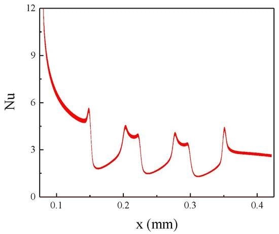
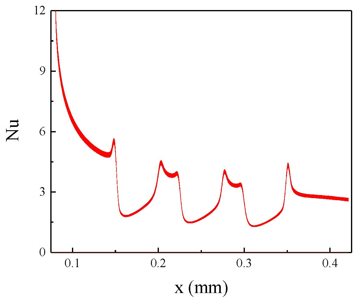
The validation of the accuracy and effectiveness of IM are demonstrated by a comparison with SM. The two methods are both free of the probability distributions of the uncertain variables. A deviation of 10% in solid volume fraction is considered, which means ${\xi }_{\varphi }^I=\left[4.5\%,5.5\%\right]$. Comparisons between the results of IM and SM are summarized in

Table 4. Bounds of variables with 10% deviation in φ.

Item	Bound	SM (100 Samples)	IM (5 Samples)
		Value	Value	Error
Temperature/K	LB	296.378	296.377	−2.558 × 10−06
	UB	296.568	296.572	1.411 × 10−05
Velocity/m·s−1	LB	1.989	1.989	1.407 × 10−05
	UB	2.180	2.180	−2.026 × 10−05
Num	LB	3.635	3.635	−6.301 × 10−05
	UB	3.835	3.835	−7.172 × 10−06

. A good agreement can be observed in Table 4, which proves the accuracy of IM. Wherein, LB and UB denote the lower bound and the upper bound, respectively. There are 100 samples used in the prediction procedure by employing SM while only five samples are used by using IM, which proves the effectiveness of IM. The variation of temperature and velocity of nanofluid on a featured line (y = 15 μm) are shown in Figure 3. In general, due to the forced convection, the temperature increases with the x-coordinate. The velocity decreases as the height of the microchannel increases and vice versa. The interval variable in solid volume fraction hardly changes the trend of temperature and velocity, and obvious bounds in temperature and velocity can be observed. Similarly, obvious bounds in the local Nusselt number of the walls can be observed in Figure 4. The local Nusselt number decreases at the grooves and the width of the bounds of the local Nusselt number is relatively small when the nanofluid enters and leaves the grooves.

3.2. The Effects of Single Uncertainty

The single uncertainty of the physical property of nanofluid has been analyzed in the last section. Thus, another type of uncertainty is considered in this section. As the manufacturing error constantly happens, the uncertainty in geometric parameter of the microchannel needs to be taken into account. To demonstrate the effect of manufacturing error, the uncertainty in the depth of the groove is considered. A deviation of 20% in the depth of the groove is chosen. Comparisons between the results of IM and those of SM are summarized in

Table 5. Bounds of variables with 20% deviation in δ.

Item	Bound	SM (100 Samples)	IM (5 Samples)
		Value	Value	Error
Temperature/K	LB	296.436	296.435	−3.007 × 10−06
	UB	296.511	296.510	−2.993 × 10−06
Velocity/m·s−1	LB	2.082	2.082	0.000
	UB	2.082	2.082	0.000
Num	LB	3.647	3.647	−1.104 × 10−04
	UB	3.826	3.826	−2.270 × 10−06

. A good agreement can be observed in Table 5, which proves the accuracy of IM. The uncertain temperature, velocity, and local Nusselt number solutions are shown in Figure 5 and Figure 6. Different from the effects of uncertainty in φ, the depth of the groove seems to have significant influence only on the variables of the local region while the solid volume fraction can influence the variables of the global region. The bound of temperature and velocity in Figure 5 is narrower than that in Figure 3, which means the depth of the grooves has a lesser impact on the temperature and velocity of nanofluid than that of the solid volume fraction of nanofluid. The depth of the grooves just arouses obvious variation of velocity and the local Nusselt number where the groove occurs. In addition, for the local Nusselt number, the upper wall presents a more obvious variation than the lower wall. In general, the uncertainty in the depth of the groove has a less impact on the thermal performance and flow behavior than that of the solid volume fraction of nanofluid.

3.3. The Effects of Two Uncertainties

When uncertainties exist in both the physical property of nanofluid and the geometric parameter, the situation becomes more serious than that when a single uncertainty happens. Deviations in solid volume fraction and the depth of the grooves are selected as 10% and 20%, respectively. Comparisons between the results of IM and those of SM are summarized in

Table 6. Bounds of variables with 10% deviation in φ and 20% deviation in δ.

Item	Bound	SM (10000 Samples)	IM (25 Samples)
		Value	Value	Error
Temperature/K	LB	296.343	296.343	−1.602 × 10−06
	UB	296.608	296.612	1.467 × 10−05
Velocity/m·s−1	LB	1.989	1.990	3.576 × 10−04
	UB	2.180	2.180	−3.860 × 10−04
Num	LB	3.545	3.541	−2.860 × 10−03
	UB	3.939	3.940	2.289 × 10−03

, and a good agreement is shown between the bounds predicted by the two methods, which proves the accuracy of IM. There are 10,000 samples used in the prediction procedure by employing SM while only 25 samples are used by using IM, which proves the effectiveness of IM. The results of the uncertain temperature, velocity, and local Nusselt number are shown in Figure 7 and Figure 8, and results of a deviation of 10% in the solid volume fraction are shown for comparison. Wherein, the two cases are referred to as Case 2 and Case 1, respectively. The deviation in both the solid volume fraction and the depth of the grooves slightly widen the bounds of temperature of Case 1 in Figure 7. And the difference between the bounds of temperature of Case 1 and Case 2 increase as the x coordinate increases. The two uncertainties in Case 2 lead to a wider bound of velocity than that of Case 1, only at which the groove occurs, and the bounds of velocity is hardly changed in other places. Conclusions can be drawn that the uncertain temperature and velocity is dominated by the deviation in the solid volume fraction. For the local Nusselt number in Figure 8, the two uncertainties in Case 2 remarkably influence the local Nusselt number of groove position on the upper wall. On the upper wall, the uncertain local Nusselt number at the grooves is dominated by the deviation in the depth of the grooves while the local Nusselt number in other places is dominated by the deviation in solid volume fraction. However, on the lower wall, bounds of the local Nusselt number caused by the two uncertainties are just slightly wider than that of Case 1, which means the uncertain local Nusselt number is dominated by the deviation in the solid volume fraction. This is because the grooves on the upper wall are far away from the lower wall.

4. Conclusions

Based on the Chebyshev polynomial approximation, IM is proposed to analyze the uncertain thermal performance and flow behavior of forced convection of nanofluid flow in a grooved microchannel. By comparing the results of IM and those of SM, it has been proved that IM can accurately and effectively predict the bounds of the interested parameters. Then, the uncertain forced convection problem under interval uncertainties in the solid volume fraction, the depth of the grooves, and their combination are investigated numerically. The results show that the uncertainties have remarkable influences on the simulated temperature, velocity, and local Nusselt number of the forced convection problem. In general, the influence of the uncertainty in the solid volume fraction is wider and greater than that of the uncertainty in the depth of the grooves.

References

- Xuan, Y.; Roetzel, W. Conceptions for heat transfer correlation of nanofluids. Int. J. Heat Mass Transf. 2000, 43, 3701–3707. [Google Scholar] [CrossRef]
- Maïga, S.E.B.; Palm, S.J.; Cong, T.N.; Roy, G.; Galanis, N. Heat transfer enhancement by using nanofluids in forced convection flows. Int. J. Heat Fluid Flow 2005, 26, 530–546. [Google Scholar] [CrossRef]
- Yurong, H.E.; Jin, Y.I.; Chen, H.; Ding, Y.; Cang, D.; Huilin, L.U. Heat transfer and flow behaviour of aqueous suspensions of TiO2 nanoparticles (nanofluids) flowing upward through a vertical pipe. Int. J. Heat Mass Transf. 2007, 50, 2272–2281. [Google Scholar]
- Heris, S.Z.; Esfahany, M.N.; Etemad, S.G. Experimental investigation of convective heat transfer of al2o3/water nanofluid in circular tube. Int. J. Heat Fluid Flow 2007, 28, 203–210. [Google Scholar] [CrossRef]
- Abu-Nada, E.; Masoud, Z.; Hijazi, A. Natural convection heat transfer enhancement in horizontal concentric annuli using nanofluids. Int. Commun. Heat Mass Transf. 2008, 35, 657–665. [Google Scholar] [CrossRef]
- Jung, J.Y.; Oh, H.S.; Kwak, H.Y. Forced convective heat transfer of nanofluids in microchannels. Int. J. Heat Mass Transf. 2006, 52, 466–472. [Google Scholar] [CrossRef]
- Hwang, K.S.; Jang, S.P.; Sus, C. Flow and convective heat transfer characteristics of water-based Al2O3 nanofluids in fully developed laminar flow regime. Int. J. Heat Mass Transf. 2009, 52, 193–199. [Google Scholar] [CrossRef]
- Duangthongsuk, W.; Wongwises, S. An experimental study on the heat transfer performance and pressure drop of tio 2-water nanofluids flowing under a turbulent flow regime. Int. J. Heat Mass Transf. 2010, 53, 334–344. [Google Scholar] [CrossRef]
- Duangthongsuk, W.; Wongwises, S. Heat transfer enhancement and pressure drop characteristics of TiO2–water nanofluid in a double-tube counter flow heat exchanger. Int. J. Heat Mass Transf. 2009, 52, 2059–2067. [Google Scholar] [CrossRef]
- Akbari, O.A.; Toghraie, D.; Karimipour, A.; Safaei, M.R.; Goodarzi, M.; Alipour, H.; Dahari, M. Investigation of rib’s height effect on heat transfer and flow parameters of laminar water–Al2O3 nanofluid in a rib-microchannel. Appl. Math. Comput. 2016, 290, 135–153. [Google Scholar]
- Sekrani, G.; Poncet, S. Further investigation on laminar forced convection of nanofluid flows in a uniformly heated pipe using direct numerical simulations. Appl. Sci.-Basel 2016, 6, 332. [Google Scholar] [CrossRef]
- Hussain, S.; Aziz, A.; Aziz, T.; Khalique, C.M. Slip flow and heat transfer of nanofluids over a porous plate embedded in a porous medium with temperature dependent viscosity and thermal conductivity. Appl. Sci.-Basel 2016, 6, 376. [Google Scholar] [CrossRef]
- Fetecau, C.; Vieru, D.; Azhar, W.A. Natural convection flow of fractional nanofluids over an isothermal vertical plate with thermal radiation. Appl. Sci.-Basel 2017, 7, 247. [Google Scholar] [CrossRef]
- Zhao, N.B.; Li, Z.M. Viscosity prediction of different ethylene glycol/water based nanofluids using a rbf neural network. Appl. Sci.-Basel 2017, 7, 409. [Google Scholar] [CrossRef]
- Williams, M.M.R. A probabilistic study of the influence of parameter uncertainty on thermal radiation heat transfer. Int. J. Heat Mass Transf. 2010, 53, 1461–1472. [Google Scholar] [CrossRef]
- Nicolaï, B.M.; Egea, J.A.; Scheerlinck, N.; Banga, J.R.; Datta, A.K. Fuzzy finite element analysis of heat conduction problems with uncertain parameters. J. Food Eng. 2011, 103, 38–46. [Google Scholar] [CrossRef]
- Wang, C. Interval analysis of steady-state heat convection–diffusion problem with uncertain-but-bounded parameters. Int. J. Heat Mass Transf. 2015, 91, 355–362. [Google Scholar] [CrossRef]
- Abdelaziz, O.; Radermacher, R. Modeling heat exchangers under consideration of manufacturing tolerances and uncertain flow distribution. Int. J. Refrig. 2010, 33, 815–828. [Google Scholar] [CrossRef]
- Xiu, D.; Karniadakis, G.E. Modeling uncertainty in steady state diffusion problems via generalized polynomial chaos. Comput. Methods Appl. Mech. Eng. 2002, 191, 4927–4948. [Google Scholar] [CrossRef] [Green Version]
- Xiu, D.; Karniadakis, G.E. A new stochastic approach to transient heat conduction modeling with uncertainty. Int. J. Heat Mass Transf. 2003, 46, 4681–4693. [Google Scholar] [CrossRef]
- Zadeh, L.A. Fuzzy sets. Inf. Control 1965, 8, 338–353. [Google Scholar] [CrossRef] [Green Version]
- Pereira, S.C.; Mello, U.T.; Ebecken, N.F.F.; Muhanna, R.L. Uncertainty in thermal basin modeling: An interval finite element approach. Reliab. Comput. 2006, 12, 451–470. [Google Scholar] [CrossRef]
- Villacci, D.; Vaccaro, A. Transient tolerance analysis of power cables thermal dynamic by interval mathematic. Electr. Power Syst. Res. 2007, 77, 308–314. [Google Scholar] [CrossRef]
- Xue, Y.; Yang, H. Interval estimation of convection-diffusion heat transfer problems. Numer. Heat Transf. Part B Fundam. 2013, 64, 263–273. [Google Scholar] [CrossRef]
- Wang, C.; Qiu, Z.; Xu, M. Collocation methods for fuzzy uncertainty propagation in heat conduction problem. Int. J. Heat Mass Transf. 2017, 107, 631–639. [Google Scholar] [CrossRef]
- Xia, B.; Yu, D.; Liu, J. Interval and subinterval perturbation methods for a structural-acoustic system with interval parameters. J. Fluids Struct. 2013, 38, 146–163. [Google Scholar] [CrossRef]
- Qiu, Z.; Wang, X. Parameter perturbation method for dynamic responses of structures with uncertain-but-bounded parameters based on interval analysis. Int. J. Solids Struct. 2005, 42, 4958–4970. [Google Scholar] [CrossRef]
- Qiu, Z.; Yi, M.; Wang, X. Comparison between non-probabilistic interval analysis method and probabilistic approach in static response problem of structures with uncertain-but-bounded parameters. Commun. Numer. Methods Eng. 2010, 20, 279–290. [Google Scholar] [CrossRef]
- Ma, Y.H.; Liang, Z.C.; Chen, M.; Hong, J. Interval analysis of rotor dynamic response with uncertain parameters. J. Sound Vib. 2013, 332, 3869–3880. [Google Scholar] [CrossRef]
- Fu, C.; Ren, X.M.; Yang, Y.F.; Qin, W.Y. Dynamic response analysis of an overhung rotor with interval uncertainties. Nonlinear Dyn. 2017, 89, 2115–2124. [Google Scholar] [CrossRef]
- Wang, C.; Ma, Y.H.; Zhang, D.Y.; Hong, J. Interval Analysis on Aero-Engine Rotor System with Misalignment. In ASME Turbo Expo 2015: Turbine Technical Conference and Exposition; Amer Soc Mechanical Engineers: New York, NY, USA, 2015. [Google Scholar]
- Ho, C.J.; Chen, M.W.; Li, Z.W. Numerical simulation of natural convection of nanofluid in a square enclosure: Effects due to uncertainties of viscosity and thermal conductivity. Int. J. Heat Mass Transf. 2008, 51, 4506–4516. [Google Scholar] [CrossRef]
- Mahian, O.; Kianifar, A.; Kleinstreuer, C.; Al-Nimr, M.D.A.; Pop, I.; Sahin, A.Z.; Wongwises, S. A review of entropy generation in nanofluid flow. Int. J. Heat Mass Transf. 2013, 65, 514–532. [Google Scholar] [CrossRef]
- Raisi, A.; Ghasemi, B.; Aminossadati, S.M. A numerical study on the forced convection of laminar nanofluid in a microchannel with both slip and no-slip conditions. Numerical Heat Transf. 2011, 59, 114–129. [Google Scholar] [CrossRef]