Computer-Aided Analysis of Gland-Like Subsurface Hyposcattering Structures in Barrett’s Esophagus Using Optical Coherence Tomography

Featured Application

The proposed image analysis algorithm can be potentially used to investigate the roles of gland-like subsurface hyposcattering structures in the progression of Barrett’s esophagus and treatment response in vivo using optical coherence tomography.

Abstract

(1) Background: Barrett’s esophagus (BE) is a complication of chronic gastroesophageal reflux disease and is a precursor to esophageal adenocarcinoma. The clinical implication of subsurface glandular structures of Barrett’s esophagus is not well understood. Optical coherence tomography (OCT), also known as volumetric laser endomicroscopy (VLE), can assess subsurface glandular structures, which appear as subsurface hyposcattering structures (SHSs). The aim of this study is to develop a computer-aided algorithm and apply it to investigate the characteristics of SHSs in BE using clinical VLE data; (2) Methods: SHSs were identified with an initial detection followed by machine learning. Comprehensive SHS characteristics including the number, volume, depth, size and shape were quantified. Clinical VLE datasets collected from 35 patients with a history of dysplasia undergoing BE surveillance were analyzed to study the general SHS distribution and characteristics in BE. A subset of radiofrequency ablation (RFA) patient data were further analyzed to investigate the pre-RFA SHS characteristics and post-RFA treatment response; (3) Results: SHSs in the BE region were significantly shallower, more vertical, less eccentric, and more regular, as compared with squamous SHSs. SHSs in the BE region which became neosquamous epithelium after RFA were shallower than those in the regions that remained BE. Pre-ablation squamous SHSs with higher eccentricity correlated strongly with larger reduction of post-ablation BE length for less elderly patients; (4) Conclusions: The computer algorithm is potentially a valuable tool for studying the roles of SHSs in BE.

1. Introduction

Barrett’s esophagus (BE), a complication of chronic gastroesophageal reflux disease, and in which the normal squamous epithelium of the esophagus is replaced by metaplastic columnar epithelium, is associated with an increased risk of esophageal carcinoma [1,2,3]. Radiofrequency ablation (RFA) is a widely used method to treat BE [1,3,4]. Multicenter clinical studies have demonstrated that RFA safely and effectively eradicates intestinal metaplasia and dysplasia [5]. However, repeated RFA over multiple treatment sessions is usually required to achieve complete remission of intestinal metaplasia (CRIM) and there is recurrence of BE even after achieving CRIM [3]. A recent multi-center study found that 33% of CRIM patients had BE recurrence within the next 2 years [6]. Standard white light endoscopy visualizes only the esophageal surface, and is unable to discern deeper gland-like structures.

Optical coherence tomography (OCT) can image 1–2 mm under the tissue surface over a broad area with micrometer-scale resolution [7,8,9] and is a promising technology for assessment of BE and dysplasia. Using a prototype OCT system, we previously [10] reported the presence of sparsely distributed subsurface hyposcattering structures (SHS) (described as “buried glands” in this reference) before and after RFA located near the gastroesophageal junction (GEJ), and suggested their presence as a negative predictive marker for achieving neosquamous epithelialization after RFA. A commercially available OCT system, known as volumetric laser endomicroscopy (VLE), can image a large field of view (6 cm × 6 cm) with a balloon catheter. Using VLE, Swager et al. [11] localized SHSs in patients previously treated with RFA for BE with high grade dysplasia or early adenocarcinoma and found that 92.4% of the SHSs were associated with normal anatomic structures, such as dilated glands and blood vessels. A later study [12] correlated VLE images from endoscopic resection specimens with histology findings and found that the presence of irregular, dilated glands/ducts is an independent predictor for BE neoplasia. The exact roles of SHSs in BE remain to be elucidated. The SHS analysis in these studies was performed manually, which is time-intensive, and is associated with inter-observer variability, as shown in recent clinical studies for detection of BE with dysplasia [13,14]. There is an unmet need for automated computer algorithms which can be applied to larger scale clinical data for faster analysis without inter-observer variability.

Qi et al. [15,16] pioneered computer-aided detection of dysplasia in BE using a standard machine learning framework and a prototype research OCT system. Ughi et al. [17] developed an algorithm based on individual axial scan analysis to characterize the esophageal wall as normal vs. BE using an OCT capsule. It is unclear whether these methods can be applied to more widely available VLE data, which are acquired with a balloon imaging device with different imaging parameters. Swager et al. [18] used clinically inspired features to train a classifier which was able to classify pre-selected ex vivo VLE images into non-dysplastic BE and neoplastic groups with a high sensitivity and specificity. However, the performance for in vivo VLE volumetric data is yet to be tested. None of the above methods were able to automatically quantify SHSs.

In this study, we therefore aimed to automate SHS analysis for clinical VLE data and quantify the characteristics of SHSs in patients with BE. We first developed a fully automated algorithm to detect and quantify SHSs and validated the algorithm by comparing to expert manual analysis. Next, we investigated the general distribution and characteristics of SHSs in patients with BE, the association between pre-ablation SHSs under the BE region and treatment response in BE patients ablated with RFA, and the correlation between pre-ablation subsquamous SHS characteristics with BE length reduction after RFA.

2. Materials and Methods

2.1. Patient Population and VLE Data

We collected VLE data from 35 patients with a history of dysplasia undergoing BE surveillance at the VA Boston Healthcare System (VABHS) from 7/2014 to 11/2016 using a commercial VLE system (NinePoint Medical, Bedford, MA, USA). The demographic and clinical information of the patients are summarized in

Table 1. Patient demographics (n = 35).

Age, mean ± STD	69.4 ± 9.3
Male, n (%)	33 (94.3%)
Race, white, n (%)	34 (97.1%)
BE length, cm, mean ± STD	2.1 ± 2.0
Treatment naïve patients, n (%) 1	8 (22.9%)
Number of prior RFA sessions, n, mean ± STD	1.7 ± 2.0
Highest pathology record of LGD, n (%) 2	18 (51.4%)
Highest pathology record of HGD/IMC, n (%) 2	14 (40%)

¹ Treatment naïve excludes all endoscopic treatment including radio-frequency ablation (RFA), cryospray ablation (CSA) and endoscopic mucosal resection (EMR). ² The pathology was obtained from biopsy or EMR specimens taken from patients. The highest pathology was selected from all the available records for a particular patient. Since each patient may have multiple visits for repeated treatments, the time of VLE imaging may not correspond to the time when the highest pathology was diagnosed. STD: standard deviation. LGD: low-grade dysplasia, HGD: high-grade dysplasia, IMC: intramucosal carcinoma.

. The study was approved by the institutional review boards at VABHS, Harvard Medical School, and Massachusetts Institute of Technology. Written informed consent was obtained from all patients prior to VLE imaging. A balloon catheter with a 20 mm diameter was introduced across the gastro-esophageal junction (GEJ) under esophagogastroduodenoscopy (EGD) guidance. After a scout OCT scan ensuring an adequate positioning of the balloon catheter, a dense 90 s pullback scan was performed, which acquired 1200 cross-sectional images with a sampling density of 50 μm/image. The axial and lateral resolutions of the system were 7 and 40 μm, respectively. More details of the VLE system can be found in other publications [19]. After VLE imaging, standard endoscopic therapy was performed based on clinical indications from endoscopy. Histology was assessed from biopsies or endoscopic mucosal resections (EMR), but with no registration with VLE. Some patients may have had more than one visit for repeated treatments and therefore multiple VLE data sets were available from different visits. However, only the VLE data during the first visit within the study time frame was used for analysis. It should also be noted that some patients enrolled for this study were not treatment naïve and had already undergone endoscopic therapy (Table 1).

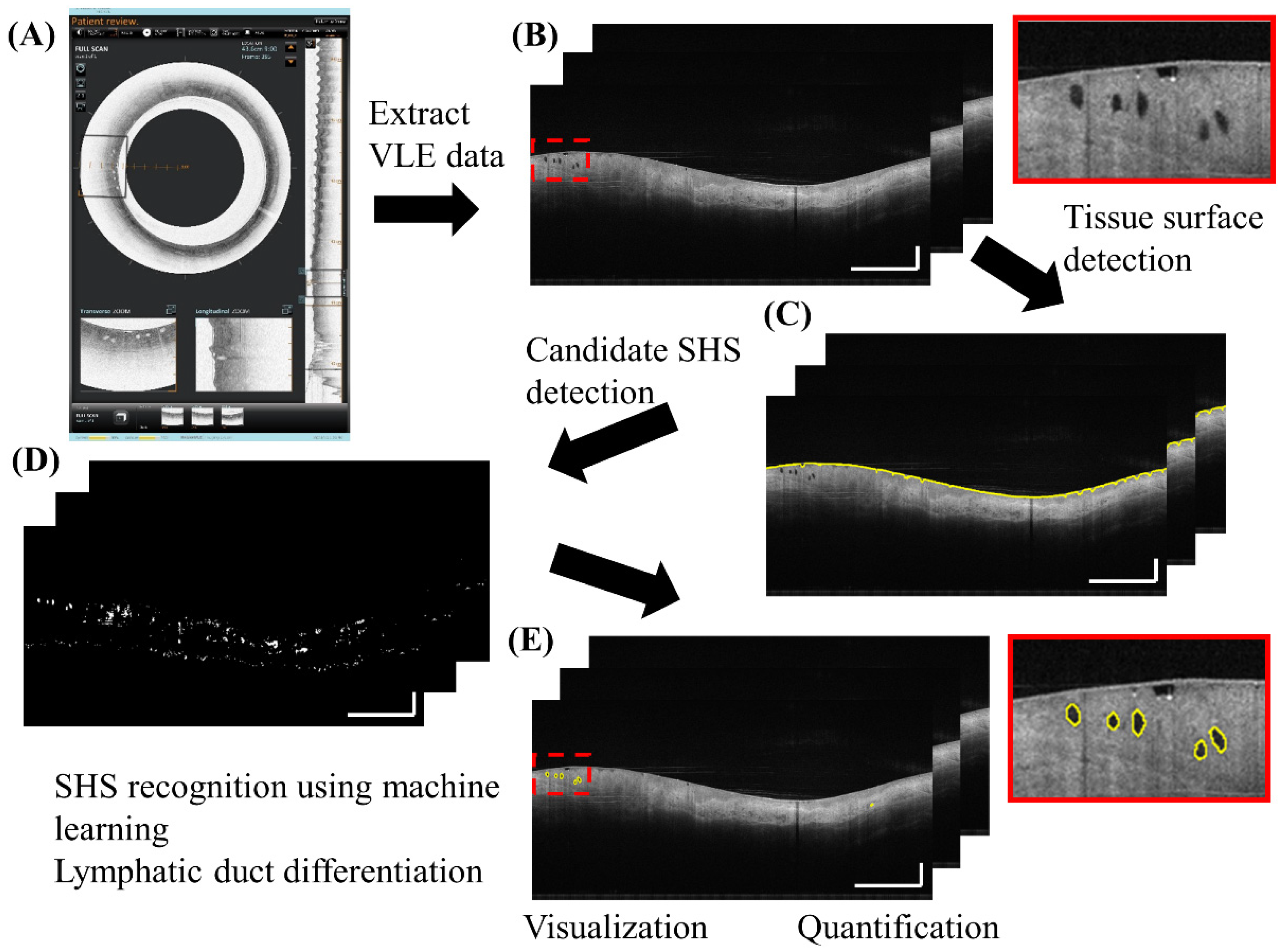
2.2. Fully Automated SHS Detection and Quantification

Figure 1 gives an overview of the algorithm. The VLE data before transform to circular display was collected for analysis (Figure 1B). It should be noted that the data here were already Fourier transformed and logarithmically compressed. From the VLE data, the tissue surface was identified using a 3D graph algorithm [20] (Figure 1C). An initial detection of candidate SHSs was performed using adaptive intensity thresholding and morphological operations by searching for low intensity “voids” (Figure 1D). The “voids” were selected based on their local intensity signature: i.e., they had lower intensity than surrounding regions, and included both SHSs and non-SHSs. Non-SHSs are mucus bubbles or other image artifacts that are non-biological. SHSs further consisted of “gland-like” SHSs and lymphatic ducts and vessels. The goal of this step was to detect all possible SHSs and therefore false positives were expected. Then, a machine learning algorithm based on a support vector machine (SVM) classifier [21] was used to classify SHSs vs non-SHSs (Figure 1E). The classifier was trained using a variety of features extracted from 1018 manually segmented SHSs in a training data set consisting of 109 images from 6 VLE pullbacks. 85 out of the 109 images were selected from BE regions, whereas the remaining 24 images were from squamous esophagus regions. The labeling and segmentation of SHSs in the training data were performed by an OCT image expert using a custom computer program. For the training data all possible “SHSs” were identified and segmented without attempting to differentiate lymphatic ducts or blood vessels from glands because a widely accepted, validated criterion was unavailable at this point. To build the SVM classifier, features were extracted from each SHS in cross-sectional VLE images, which included intensity, shape (eccentricity and solidity, see Section 2.3 and Figure 2), depth and size. Additional features such as the intensity and standard deviation of the surrounding region of each SHS were also added to help differentiate SHSs from surface mucous bubbles. These features effectively removed most of the false positives. The processing steps described above were performed in 2D cross-sectional images (B-scans) without using 3D volumetric information. Although it is difficult even for human experts to differentiate lymphatic ducts and vascular structures from “gland-like” SHSs based on cross-sectional images alone, lymphatic ducts have a much longer longitudinal length extent than “gland-like” SHSs. Therefore, candidate regions longer than a threshold of 0.5 mm (10 images) were automatically classified by the algorithm as lymphatic ducts. The threshold length was pre-determined experimentally with the training data. For simplicity, “gland-like” SHSs are simply referred as SHSs in subsequent text. Currently, the entire algorithm was implemented in MATLAB for rapid development, and was not optimized for high speed processing.

We validated the SHS detection algorithm using a test dataset of 100 randomly selected images from 10 cases not in the training data. An OCT image expert manually segmented 896 SHSs from the test dataset. True positives (TP), false positives (FP) and false negatives (FN) of SHSs were calculated on a per-SHS basis by comparing the algorithm output to expert manual segmentation in individual cross-sectional images. True negatives (TN) were not informative, because any non-SHS features can be regarded as TN. SHS boundary segmentation accuracy was assessed using the Dice coefficient, defined as the intersection over the union between the automatic and manual segmentation (2 × (Auto ∩ Manual)/(Auto + Manual)), which is in the range of 0–1 (Figure 2A).

2.3. SHS Quantification

After SHSs were detected, several metrics were quantified automatically. There were two types of metrics: (1) cumulative metrics generated over a longitudinal segment of the esophagus, and (2) intensity, shape and location metrics generated on a per-SHS basis. The three cumulative metrics are:

• The 2D number: quantified as mean/cross-section
• Volume: total gland volume within the region of interest
• The 3D number (Cluster): if the distance between adjacent 2D SHSs is within 2.5 mm circumferentially (this threshold is relatively large to account for motion artifacts) and within 3 images (0.15 mm) longitudinally, these SHSs were considered as one 3D cluster.

The nine metrics generated on a per-SHS basis were either in Cartesian (C) (Figure 1A) or in Polar (P) (Figure 1B) coordinates, depending on the convenience of computation:

4.

Size: area of each SHS in 2D cross-sectional images (C)

5.

Perimeter: perimeter of each SHS in cross-sectional images (C)

Size and perimeter are related but are not necessarily correlated. An SHS with a concave, irregular shape may have a large perimeter but a small size.

6.

Depth: distance from the centroid of each SHS to the tissue surface (P)

7.

Intensity: intensity of SHS normalized by the mean intensity of the axial lines traversing the SHS to account for intensity fluctuations between different angles, images and pullbacks

8.

Standard deviation (STD): characterizing the intensity heterogeneity (P)

9.

Orientation: absolute angle between the major axis of the SHS and tissue surface (P) after flattening the image to the tissue surface (Figure 2B)

10.

Eccentricity: ratio between the foci of a fitted ellipse to the major axis length with a range of 0–1 where 0 indicates a circle and 1 indicates a line (C) (Figure 2C)

11.

Extent: ratio of SHS area to its bounding box (C), characterizing irregularity (Figure 2D)

12.

Solidity: ratio of SHS area to its convex area (C), characterizing irregularity (Figure 2E)

Extent characterizes how well a region fills in its “bounding box”, whereas solidity characterizes how convex a region is.

2.4. Applications of the Automated SHS Quantification Algorithm

To demonstrate the utility of the SHS quantification algorithm, we analyzed retrospective VLE data from BE patients to investigate the characteristics of SHSs in BE. For each VLE pullback, the maximum extent of contiguous BE (most proximal location, denoted by M) was identified manually by consensus of two OCT image experts and used as a reference for SHS quantification. Three different analysis and patient groups were employed for different purposes, detailed in Section 2.4.1, Section 2.4.2 and Section 2.4.3. Subgroup analysis stratified by the highest pathology records (low-grade dysplasia (LGD) vs high-grade dysplasia (HGD) and intramucosal carcinoma (IMC)) was also performed (Table 1, see also Tables S1–S6).

2.4.1. General Distribution and Characteristics of SHS in Patients with BE

The objective of this study was to investigate the general SHS distribution in BE as well as whether SHSs exhibit any location-specific features. Data from all patients who had VLE (n = 35) was analyzed, regardless of their endoscopy treatment and whether they had EGD follow-up. SHS quantification was performed over a 4 cm segment starting from the 1 cm BE region distal to M extending to the squamous epithelium. The SHS characteristics were compared between each 1 cm segment over the 4 cm longitudinal region (Figure 3A).

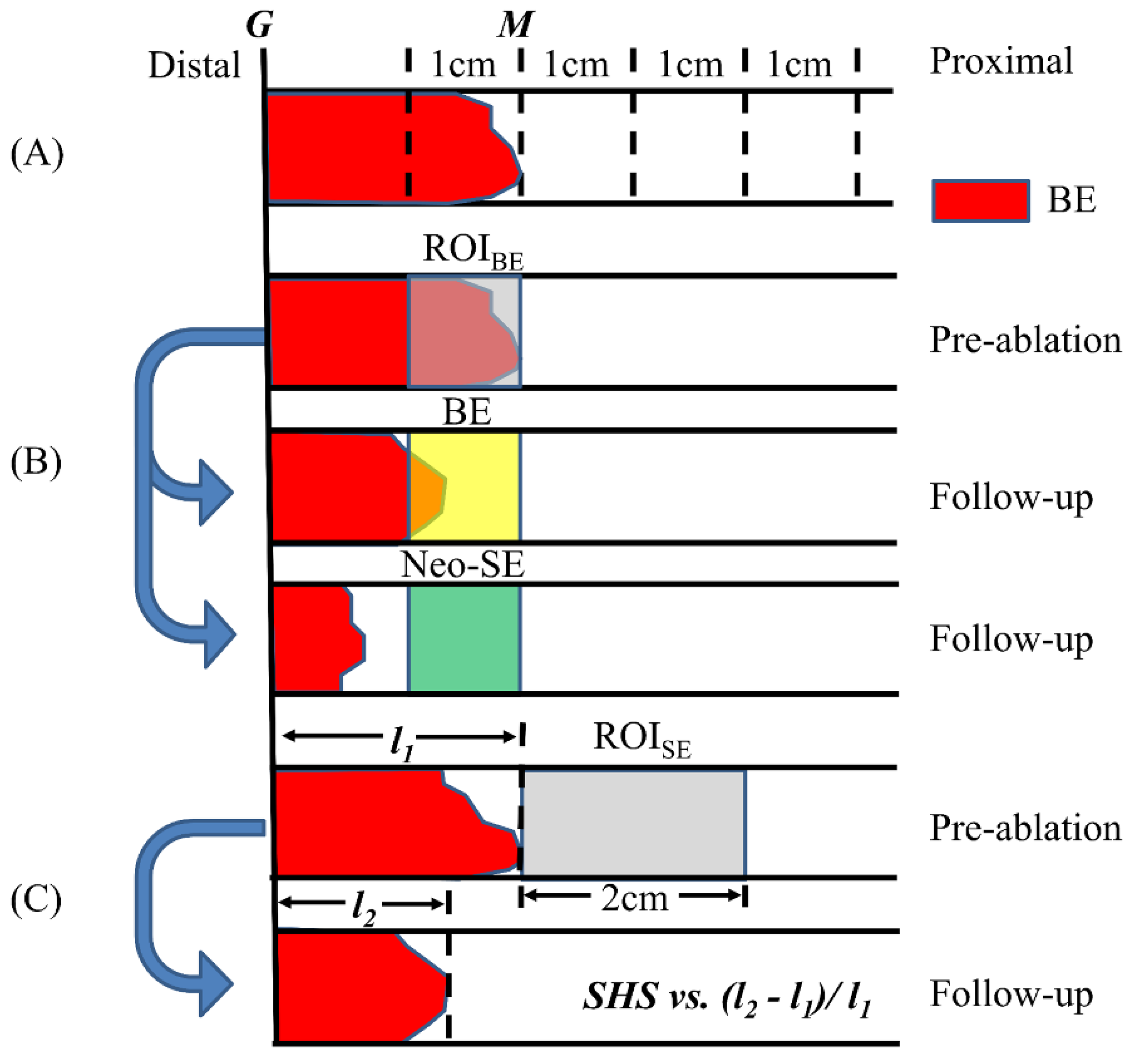
2.4.2. Pre-Ablation BE SHS and RFA Treatment Response

The objective of this study was to investigate whether SHS in the BE region was associated with RFA treatment response. Data from a subset of 21 patients imaged by VLE, treated by RFA on the same visit, and with EGD at follow-up within 1–4 months was analyzed to investigate the association between the pre-ablation BE SHS characteristics and whether the BE region achieved neosquamous epithelium. The mean age of the patients was 71.1 ± 9.7 and all were male. The mean BE length was 2.1 ± 2.3 cm.

We defined the 1 cm segment region distal to M as the BE region of interest (ROI_BE) to perform SHS quantification (Figure 3B). Note that the ROI_BE may not be entirely BE if M was not coincident with the most proximal circumferential extent of BE. The SHS characteristics quantified over this region were compared between patients whose ROI_BE had neosquamous epithelium (neo-SE) versus remaining BE at follow-up EGD. Here, the ROI_BE was required to be completely squamous epithelium to be counted as neo-SE on follow-up (Figure 3B). Therefore, the RFA treatment response here was specifically related to the post-ablation response of the 1 cm segment ROI_BE, rather than the standard definition of CRIM.

2.4.3. Pre-Ablation Subsquamous SHS Characteristics and RFA Treatment Response

The objective of this study was to investigate the association between pre-ablation squamous SHS and treatment response. Similar to the previous study, we included the same cohort of patients (n = 21). However, SHS quantification was performed within the 2 cm segment proximal to M (denoted by ROI_SE, Figure 3C). The SHS characteristics were correlated to the reduction of maximum BE length (change of M in EGD) after RFA treatment. To account for the differences in baseline BE lengths between different patients, we normalized the change of BE length by the initial BE length at the first study visit. To understand the effect of age on the treatment response, we divided the patients into ≤70 (n = 10) and >70 years old (n = 11) and analyzed the correlations separately.

2.5. Statistical Analysis

Quantitative metrics were presented as mean ± standard deviation (STD). Comparison between two groups was performed using either independent sample t-test (for normal distribution) or Mann–Whitney U Test (skewed distribution). Comparison among more than two groups was performed using Analysis of Variance (ANOVA). Correlation between quantitative metrics and treatment response was assessed using either Pearson’s product-moment correlation (for normal distribution), or Spearman’s rank-order correlation (skewed distribution or presence of outliers). A p-value < 0.05 was considered significant. All analyses were conducted in SPSS (version 18, IBM, Armonk, NY, USA).

3. Results

3.1. Performance of the Algorithm

Compared to expert manually segmented SHSs (n = 896) in 100 images from 10 cases (10 images/case), the algorithm achieved a sensitivity (TP/(TP + FN)) of 82.6%, and a positive predictive value (PPV) (TP/(TP + FP)) of 86.7% on a per-SHS basis. For correctly detected SHSs, the boundary segmentation accuracy was 90% ± 3%. The computation time of the algorithm was 3.9 s/image, tested on a 64-bit computer with a 3.2 GHz intel i7 CPU.

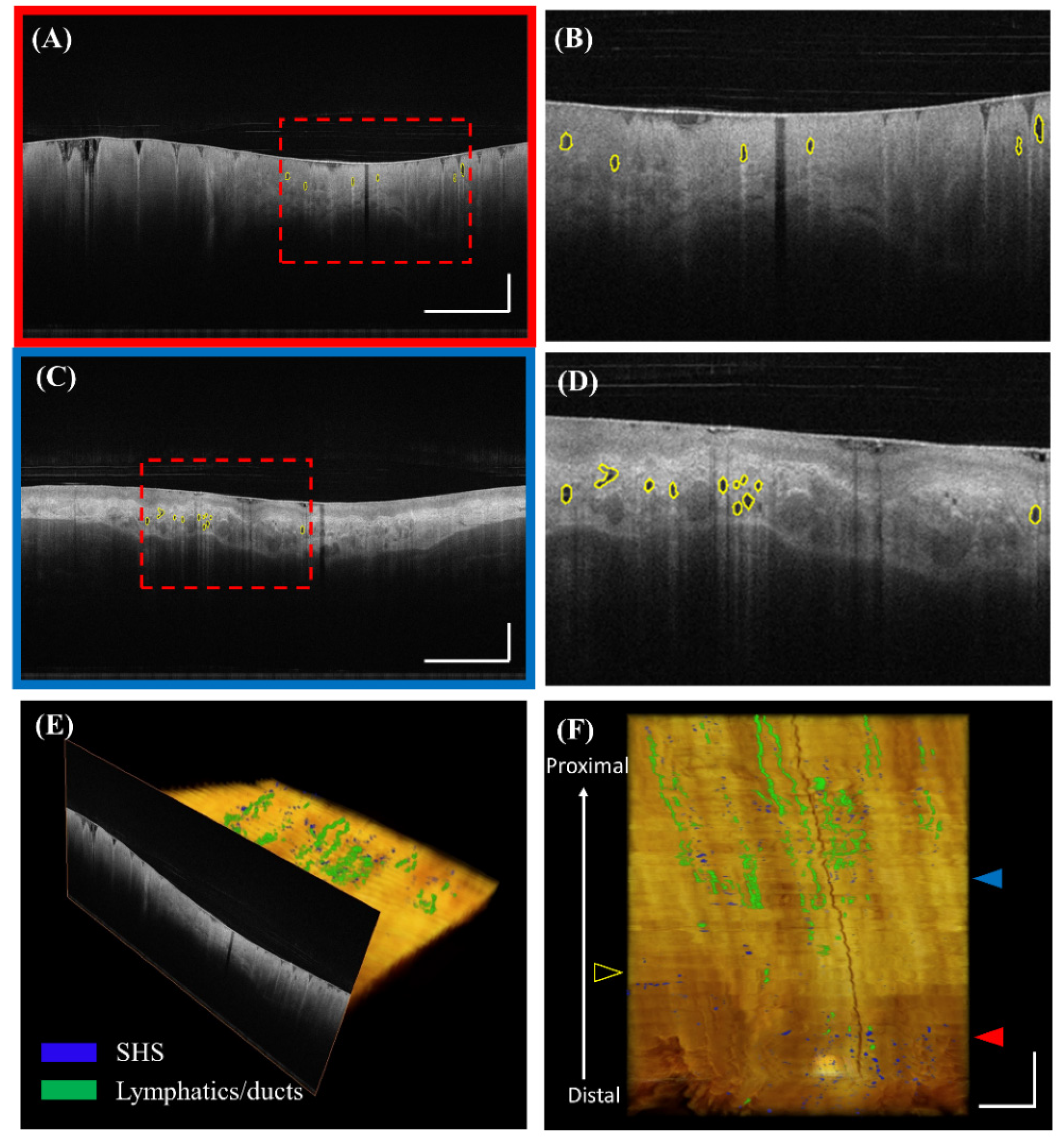
3.2. Visualization of SHS

The automatically detected SHSs can be visualized in 2D and 3D. Figure 4 illustrates an example where the SHSs were segmented and labeled by the algorithm in both BE and squamous regions. In the 3D view, the SHSs (blue) appeared as local, spotted features, whereas the lymphatics and ducts (green) formed elongated, connected “pipes” that traversed many images longitudinally.

3.3. Comparison of SHS Characteristics over the Longitudinal Segments in BE

SHSs in the BE region (Segment 1) were significantly shallower, more vertical, less eccentric, and more regular compared with those in the squamous region (Segments 2–4,

Table 2. Comparison of SHS characteristics over the 4 cm longitudinal segments in BE.

Metrics	Segment 1	Segment 2	Segment 3	Segment 4	p-Value (All)	p-Value (1 vs. 2)	p-Value (2 vs. 3)	p-Value (3 vs. 4)
2D Number	0.98 ± 0.71	1.05 ± 0.59	1.17 ± 0.64	1.14 ± 0.87	0.653	-	-	-
Volume (mm3)	2.25 ± 1.86	2.37 ± 1.84	2.32 ± 1.64	2.28 ± 1.91	0.994	-	-	-
3D Cluster	8.51 ± 7.40	11.17 ± 7.73	12.44 ± 7.72	11.17 ± 9.66	0.221	-	-	-
Size (mm2)	0.22 ± 0.07	0.24 ± 0.14	0.19 ± 0.06	0.19 ± 0.07	0.115	-	-	-
Depth (mm)	0.83 ± 0.15	0.98 ± 0.20	0.95 ± 0.12	0.87 ± 0.25	0.003 **	0.006 **	0.936	0.234
Intensity	0.64 ± 0.11	0.65 ± 0.09	0.67 ± 0.08	0.65 ± 0.18	0.793	-	-	-
STD	0.08 ± 0.01	0.08 ± 0.01	0.08 ± 0.01	0.08 ± 0.02	0.913	-	-	-
Orientation (degrees)	10.0 ± 4.6	7.9 ± 4.7	6.4 ± 2.2	7.0 ± 4.5	0.002 **	0.144	0.399	0.898
Eccentricity (0–1)	0.82± 0.07	0.90 ± 0.03	0.90 ± 0.02	0.84 ± 0.21	0.006 **	0.029 *	0.999	0.135
Extent (0–1)	0.58 ± 0.05	0.54 ± 0.04	0.54 ± 0.03	0.50 ± 0.13	<0.001 ***	0.057	1.000	0.172
Perimeter (mm)	2.02 ± 0.22	2.17 ± 0.40	2.04 ± 0.29	1.95 ± 0.54	0.110	-	-	-
Solidity (0–1)	0.90 ± 0.01	0.89 ± 0.01	0.89 ± 0.01	0.84 ± 0.21	0.080	-	-	-

). Subgroup analysis further revealed that this is the case for LGD patients, but not for HGD/IMC patients (Tables S1 and S2). The number or volume of SHSs in each 1 cm longitudinal segment, from the 1 cm BE region distal to M up to squamous epithelium, were not significantly different. Most SHS parameters in each segment were not significantly different between LGD and HGD/IMC groups (Table S3).

3.4. SHS in the BE Region and RFA Treatment Response

Table 3. Comparison of pre-radiofrequency ablation (RFA) BE SHS between patients who did and did not have RFA treatment response on follow up (achieving neosquamous epithelium).

Cumulative Metrics	Neo-SE	BE	p-Value	Neo-SE	BE	p-Value
2D number	1.04 ± 0.74	0.75± 0.24	0.221	-	-	-
3D number	8.31 ± 7.52	5.88 ± 2.80	0.860	-	-	-
Volume (mm3)	2.52 ± 2.20	1.61 ± 0.83	0.210	-	-	-
Metrics on a per gland basis	Mean of all SHSs			Mean of cross-sectional extreme
Size (mm2)	0.22 ± 0.06	0.22 ± 0.10	0.336	0.28 ± 0.12	0.26 ± 0.15	0.374
Depth (mm)	0.83 ± 0.13	0.96 ± 0.14	0.041 *	0.92 ± 0.13	1.03 ± 0.13	0.064
Intensity	0.63 ± 0.06	0.65 ± 0.11	0.598	0.69 ± 0.08	0.68 ± 0.12	0.750
STD	0.08 ± 0.01	0.08 ± 0.02	0.507	0.09 ± 0.01	0.09 ± 0.02	0.385
Orientation (degrees)	11.2 ± 4.0	8.9 ± 4.4	0.121	15.3 ± 7.8	10.9 ± 5.0	0.185
Eccentricity (0–1)	0.82 ± 0.07	0.86 ± 0.05	0.241	0.87 ± 0.06	0.87 ± 0.06	0.849
Extent (0–1)	0.60 ± 0.04	0.57 ± 0.03	0.087	0.56 ± 0.05	0.54 ± 0.04	0.363
Perimeter (mm)	2.02 ± 0.21	2.00 ± 0.25	0.087	2.27 ± 0.41	2.17 ± 0.34	0.363
Solidity (0–1)	0.90 ± 0.01	0.89 ± 0.01	0.053	0.89 ± 0.01	0.88 ± 0.01	0.238

summarizes the comparison of the SHSs in RFA ablated BE between SHSs in patients with neo-SE and BE at follow-up. For each quantitative metric, we analyzed the mean of all SHSs as well as the maximum or minimum values of individual images, namely the maximum size and depth, highest intensity and STD, maximum orientation and eccentricity, and minimum extent and solidity. Patients having BE with shallower SHSs were more likely to achieve neo-SE on follow up post-ablation (neo-SE mean value: 0.83 ± 0.13 mm vs. BE mean value: 0.96 ± 0.14 mm, p = 0.041). Noticeably, the depth difference for the treatment response was mainly driven by the HGD/IMC patients (neo-SE: 0.84 ± 0.11 mm, BE: 1.02 ± 0.13 mm, p = 0.050, Table S5) rather than LGD patients (neo-SE: 0.82 ± 0.17 mm, BE: 0.90 ± 0.14 mm, p = 0.441, Table S4). Table 3 also shows that the pre-ablation SHS solidity (regularity) in the BE region may be a predictor of post-ablation neo-SE (neo-SE: 0.90 ± 0.01, BE: 0.89 ± 0.01, p = 0.053) although it did not achieve statistical significance in this study.

3.5. SHS in the Squamous Region and RFA Treatment Response

Pre-ablation SHSs parameters were not significantly different between patients of different age groups (data not shown). Subsquamous SHSs with higher eccentricity is strongly correlated with larger reduction of post-ablation BE length for less elderly patients (≤70 years old, R = −0.884, p = 0.001,

Table 4. Correlation between pre-ablation squamous SHS metrics and the relative change of maximum BE length after RFA in different age groups.

Cumulative Metrics	Age ≤ 70 (n = 10)		Age > 70 (n = 11)		Age ≤ 70 (n = 10)		Age > 70 (n = 11)
	R	p-value	R	p-value	R	p-value	R	p-value
2D number	−0.185	0.609	0.178	0.601	-	-	-	-
3D number	−0.180	0.605	0.243	0.471	-	-	-	-
Volume (mm3)	−0.020	0.956	0.103	0.763	-	-	-	-
Metrics on a per gland basis	Mean of all SHSs				Mean of cross-sectional extreme
Size (mm2)	−0.240	0.504	−0.047	0.891	−0.246	0.493	0.047	0.891
Depth (mm)	0.129	0.722	0.327	0.326	0.228	0.527	0.365	0.270
Intensity	−0.326	0.358	−0.065	0.848	−0.062	0.866	0.122	0.722
STD	0.209	0.562	−0.065	0.848	0.129	0.722	0.019	0.956
Orientation (degrees)	0.640	0.046 *	−0.365	0.270	0.825	0.003 **	−0.327	0.326
Eccentricity (0–1)	−0.884	0.001 **	0.355	0.284	−0.850	0.002 **	0.355	0.284
Extent (0–1)	0.695	0.026 *	0.467	0.147	0.695	0.026 *	−0.514	0.106
Perimeter (mm)	−0.714	0.720	0.280	0.403	−0.480	0.160	0.234	0.489
Solidity (0–1)	0.585	0.075	0.570	0.067	0.517	0.126	−0.567	0.069

), but not for elderly patients (>70 years old, R = 0.355, p = 0.284) (Table 4). More vertical and more regular subsquamous SHSs corresponded to less reduction of post-ablation BE length for less elderly patients.

Subgroup analysis stratified by pathology revealed that SHSs in the squamous region correlate differently with post-RFA response in different patient groups. SHSs eccentricity is strongly correlated with larger reduction of post-ablation BE length for LGD patients (R = −0.829, p = 0.003, Table S6), but with less reduction of post-ablation BE length for HGD/IMC patients (R = 0.685, p = 0.029) (Table S6). Less vertical, higher intensity and STD subsquamous SHSs corresponded to less reduction of post-ablation BE length for HGD/IMC patients, but not for LGD patients (Table S6). Smaller perimeter subsquamous SHSs was correlated with less reduction of post-ablation BE length for LGD patients, but not for HGD/IMC patients (Table S6).

4. Discussion

This is the first report of a fully automated algorithm for SHS detection and quantification in OCT images acquired using the commercially available VLE instrument, without requiring any pre-selection of regions of interests or manual input. This is also the first study to apply automated algorithms to investigate the general distribution and characteristics of SHSs in Barrett’s esophagus and the association of SHSs with RFA treatment response. The algorithm can be readily applied to any existing VLE images to extract quantitative information from large amounts of data, which is impractical with manual analysis. With further speed optimization, it could also be applied for real-time analysis to provide clinical information during endoscopic procedures. The SHS quantification algorithm can also be used as an input for other computer-aided algorithms. For example, the features of SHS can be combined with other clinical features for dysplastic BE classification [18].

The conventional way to analyze SHSs is to assess their presence [9,22] or to manually count their number [10], which is time-intensive, and cannot comprehensively characterize SHSs. The algorithm developed in this study not only automates the above tasks, but augments the capability to assess additional features such as the SHS intensity, depth and shape information, which may also be clinically important. As shown in this study, we found that the depth and solidity of SHSs in the BE region were more significant indicators of post-RFA treatment response than the number. It is likely that thicker BE is harder to eradicate completely [23], and conceivable that higher SHS irregularity is associated with more advanced stage of BE. These subsurface features cannot be visualized or analyzed using conventional white light endoscopy. Barrett’s glands have been described to evolve from columnar-lined mucosa without goblet cells, to glands showing intestinal gene expression and to specialized metaplastic glands [24]. More glandular distortions such as branched or cribriform glands may have more malignant potential. The proposed algorithm can be useful to track the changes of gland characteristics and identify the early markers for metaplasia and dysplasia.

We found that the eccentricity of pre-ablation SHSs in the squamous region was strongly correlated with the reduction of BE length at follow-up (Table 4), but only for less elderly patients. This suggests that age might be an important factor that could affect the RFA treatment response. It also suggests that squamous and BE SHSs may play different roles in RFA-treated BE. One obvious difference is that BE SHSs were directly ablated during the treatment, while the squamous SHSs were not. It should be noted that in this study, the SHSs may result from previous ablations for those previously treated patients. Further studies with larger enrollment and treatment naive patients are needed to confirm the roles of squamous SHSs [25,26].

We also found that SHSs in the BE region were significantly shallower, more vertical, less eccentric and more regular compared to subsquamous SHSs (Table 2). This is likely the case because BE glands are usually found in the epithelium, but subsquamous glands are often below the epithelium. Another possible explanation is that OCT light penetration to deeper structures was more limited in the BE region compared with the squamous region. The high irregularity of SHSs in the squamous region may be associated with previous ablation treatments.

There were considerable differences for the roles of SHSs between LGD and HGD/IMC patients. For example, as shown, BE with shallower SHSs were more likely to achieve neo-SE for HGD/IMC patients. The correlations of several subsquamous SHS characteristics and the reduction of BE length were also different between HGD/IMC and LGD patients. However, the results here should be interpreted with caution because the highest pathology diagnosis may not necessarily correspond to the time of VLE imaging.

Swager et al. [11] reported that most of the SHSs in VLE are normal histological features. In this study, we applied a criterion to differentiate normal lymphatic ducts from glands based on their longitudinal axis length. Although empirical, this was effective in excluding most of the normal lymphatic ducts from glands from unwanted analysis. However, it may be difficult to differentiate between glands and vessels in VLE due to their similar intensity. Newly developed functional imaging methods such as OCT angiography can be applied to identify depth-resolved vasculature [27,28]. Moreover, we could not exclude the possibility that there might be other normal features that were detected as “gland-like” structures by the algorithm. Nevertheless, the algorithm can be used with laser marking technology [29,30] to further validate the nature of SHSs found in VLE with histopathology of co-registered excisional biopsies.

There are several limitations in this study. First, the sample size is relatively small. Second, most of the patients enrolled in this study were not treatment naïve and had relatively short segment BE. Third, the SHSs detected by the algorithm were not validated against histopathology, and the correlation between SHS findings and dysplasia cannot be established. Fourth, the study is retrospective. Lastly, VLE data has motion artifacts such as non-uniform rotational distortion (NURD). Several post-processing algorithms [31,32,33] for correcting NURD have been proposed, but methods for high accuracy and full automation are still needed. Therefore, the quantitative shape descriptor results should be interpreted as an estimate of the actual SHS morphology.

5. Conclusions

We developed a computer algorithm which enabled fully automated analysis of SHS number, size, cluster and shape. SHSs in the BE region were significantly shallower, more vertical, less eccentric, and more regular compared with SHS in the squamous region. BE with shallower, more regular subsurface SHS was more likely to achieve neosquamous epithelium after RFA. More eccentric pre-ablation SHSs in the squamous region were strongly correlated with higher reduction of post-ablation BE length for less elderly patients.

References

1. Spechler, S.J.; Souza, R.F. Barrett’s esophagus. N. Engl. J. Med. 2014, 371, 836–845. [Google Scholar] [CrossRef] [PubMed]
2. Sharma, P.; McQuaid, K.; Dent, J.; Fennerty, M.B.; Sampliner, R.; Spechler, S.; Cameron, A.; Corley, D.; Falk, G.; Goldblum, J.; et al. A critical review of the diagnosis and management of Barrett’s esophagus: The AGA Chicago Workshop. Gastroenterology 2004, 127, 310–330. [Google Scholar] [CrossRef] [PubMed]
3. Shaheen, N.J.; Falk, G.W.; Iyer, P.G.; Gerson, L.B.; American College of Gastroenterology. ACG clinical guideline: Diagnosis and management of Barrett’s esophagus. Am. J. Gastroenterol. 2016, 111, 30–50. [Google Scholar] [CrossRef] [PubMed]
4. Orman, E.S.; Li, N.; Shaheen, N.J. Efficacy and durability of radiofrequency ablation for Barrett’s Esophagus: Systematic review and meta-analysis. Clin. Gastroenterol. Hepatol. 2013, 11, 1245–1255. [Google Scholar] [CrossRef] [PubMed]
5. Shaheen, N.J.; Sharma, P.; Overholt, B.F.; Wolfsen, H.C.; Sampliner, R.E.; Wang, K.K.; Galanko, J.A.; Bronner, M.P.; Goldblum, J.R.; Bennett, A.E.; et al. Radiofrequency Ablation in Barrett’s Esophagus with Dysplasia. N. Engl. J. Med. 2009, 360, 2277–2288. [Google Scholar] [CrossRef] [PubMed]
6. Gupta, M.; Iyer, P.G.; Lutzke, L.; Gorospe, E.C.; Abrams, J.A.; Falk, G.W.; Ginsberg, G.G.; Rustgi, A.K.; Lightdale, C.J.; Wang, T.C.; et al. Recurrence of esophageal intestinal metaplasia after endoscopic mucosal resection and radiofrequency ablation of Barrett’s esophagus: Results from a US Multicenter Consortium. Gastroenterology 2013, 145, 79–86. [Google Scholar] [CrossRef] [PubMed]
7. Tearney, G.J.; Brezinski, M.E.; Bouma, B.E.; Boppart, S.A.; Pitris, C.; Southern, J.F.; Fujimoto, J.G. In vivo endoscopic optical biopsy with optical coherence tomography. Science 1997, 276, 2037–2039. [Google Scholar] [CrossRef] [PubMed]
8. Isenberg, G.; Sivak, M.V., Jr.; Chak, A.; Wong, R.C.; Willis, J.E.; Wolf, B.; Rowland, D.Y.; Das, A.; Rollins, A. Accuracy of endoscopic optical coherence tomography in the detection of dysplasia in Barrett’s esophagus: A prospective, double-blinded study. Gastrointest. Endosc. 2005, 62, 825–831. [Google Scholar] [CrossRef] [PubMed]
9. Evans, J.A.; Poneros, J.M.; Bouma, B.E.; Bressner, J.; Halpern, E.F.; Shishkov, M.; Lauwers, G.Y.; Mino-Kenudson, M.; Nishioka, N.S.; Tearney, G.J. Optical Coherence Tomography to Identify Intramucosal Carcinoma and High-Grade Dysplasia in Barrett’s Esophagus. Clin. Gastroenterol. Hepatol. 2006, 4, 38–43. [Google Scholar] [CrossRef] [Green Version]
10. Zhou, C.; Tsai, T.H.; Lee, H.C.; Kirtane, T.; Figueiredo, M.; Tao, Y.K.; Ahsen, O.O.; Adler, D.C.; Schmitt, J.M.; Huang, Q.; et al. Characterization of buried glands before and after radiofrequency ablation by using 3-dimensional optical coherence tomography (with videos). Gastrointest. Endosc. 2012, 76, 32–40. [Google Scholar] [CrossRef] [PubMed] [Green Version]
11. Swager, A.F.; Boerwinkel, D.F.; de Bruin, D.M.; Faber, D.J.; van Leeuwen, T.G.; Weusten, B.L.; Meijer, S.L.; Bergman, J.J.; Curvers, W.L. Detection of buried Barrett’s glands after radiofrequency ablation with volumetric laser endomicroscopy. Gastrointest. Endosc. 2016, 83, 80–88. [Google Scholar] [CrossRef] [PubMed]
12. Swager, A.F.; Tearney, G.J.; Leggett, C.L.; van Oijen, M.G.H.; Meijer, S.L.; Weusten, B.L.; Curvers, W.L.; Bergman, J.J. Identification of volumetric laser endomicroscopy features predictive for early neoplasia in Barrett’s esophagus using high-quality histological correlation. Gastrointest. Endosc. 2017, 85, 918–926. [Google Scholar] [CrossRef] [PubMed]
13. Leggett, C.L.; Gorospe, E.C.; Chan, D.K.; Muppa, P.; Owens, V.; Smyrk, T.C.; Anderson, M.; Lutzke, L.S.; Tearney, G.; Wang, K.K. Comparative diagnostic performance of volumetric laser endomicroscopy and confocal laser endomicroscopy in the detection of dysplasia associated with Barrett’s esophagus. Gastrointest. Endosc. 2016, 83, 880–888. [Google Scholar] [CrossRef] [PubMed]
14. Lee, H.C.; Ahsen, O.O.; Liang, K.; Figueiredo, M.; Giacomelli, M.G.; Potsaid, B.; Huang, Q.; Mashimo, H.; Fujimoto, J.G. Endoscopic optical coherence tomography angiography microvascular features associated with dysplasia in Barrett’s esophagus (with video). Gastrointest. Endosc. 2017, 86, 476–484. [Google Scholar] [CrossRef] [PubMed]
15. Qi, X.; Sivak, M.V.; Isenberg, G.; Willis, J.E.; Rollins, A.M. Computer-aided diagnosis of dysplasia in Barrett’s esophagus using endoscopic optical coherence tomography. J. Biomed. Opt. 2006, 11, 044010. [Google Scholar] [CrossRef] [PubMed]
16. Qi, X.; Pan, Y.; Sivak, M.V.; Isenberg, G.; Rollins, A.M. Image analysis for classification of dysplasia in Barrett’s esophagus using endoscopic optical coherence tomography. Biomed. Opt. Express 2010, 1, 825–847. [Google Scholar] [CrossRef] [PubMed]
17. Ughi, G.J.; Gora, M.J.; Swager, A.F.; Soomro, A.; Grant, C.; Tiernan, A.; Rosenberg, M.; Sauk, J.S.; Nishioka, N.S.; Tearney, G.J. Automated segmentation and characterization of esophageal wall in vivo by tethered capsule optical coherence tomography endomicroscopy. Biomed. Opt. Express 2016, 7, 409–419. [Google Scholar] [CrossRef] [PubMed]
18. Swager, A.F.; van der Sommen, F.; Klomp, S.R.; Zinger, S.; Meijer, S.L.; Schoon, E.J.; Bergman, J.J.; de With, P.H.; Curvers, W.L. Computer-aided detection of early Barrett’s neoplasia using volumetric laser endomicroscopy. Gastrointest. Endosc. 2017, 86, 839–846. [Google Scholar] [CrossRef] [PubMed] [Green Version]
19. Wolfsen, H.C.; Sharma, P.; Wallace, M.B.; Leggett, C.; Tearney, G.; Wang, K.K. Safety and feasibility of volumetric laser endomicroscopy in patients with Barrett’s esophagus (with videos). Gastrointest. Endosc. 2015, 82, 631–640. [Google Scholar] [CrossRef] [PubMed]
20. Li, K.; Wu, X.; Chen, D.Z.; Sonka, M. Optimal Surface Segmentation in Volumetric Images—A Graph-Theoretic Approach. IEEE. Trans. Pattern Anal. Mach. Intell. 2006, 28, 119–134. [Google Scholar] [PubMed]
21. Chang, C.C.; Lin, C.J. LIBSVM: A library for support vector machines. ACM. Trans. Intell. Syst. Technol. 2011, 2, 27. [Google Scholar] [CrossRef]
22. Evans, J.A.; Bouma, B.E.; Bressner, J.; Shishkov, M.; Lauwers, G.Y.; Mino-Kenudson, M.; Nishioka, N.S.; Tearney, G.J. Identifying intestinal metaplasia at the squamocolumnar junction by using optical coherence tomography. Gastrointest. Endosc. 2007, 65, 50–56. [Google Scholar] [CrossRef] [PubMed] [Green Version]
23. Tsai, T.H.; Zhou, C.; Tao, Y.K.; Lee, H.C.; Ahsen, O.O.; Figueiredo, M.; Kirtane, T.; Adler, D.C.; Schmitt, J.M.; Huang, Q.; et al. Structural markers observed with endoscopic 3-dimensional optical coherence tomography correlating with Barrett’s esophagus radiofrequency ablation treatment response (with videos). Gastrointest. Endosc. 2012, 76, 1104–1112. [Google Scholar] [CrossRef] [PubMed]
24. McDonald, S.A.; Graham, T.A.; Lavery, D.L.; Wright, N.A.; Jansen, M. The Barrett’s Gland in Phenotype Space. Cell Mol. Gastroenterol. Hepatol. 2015, 1, 41–54. [Google Scholar] [CrossRef] [PubMed] [Green Version]
25. Yachimski, P.; Falk, G.W. Subsquamous intestinal metaplasia: Implications for endoscopic management of Barrett’s esophagus. Clin. Gastroenterol. Hepatol. 2012, 10, 220–224. [Google Scholar] [CrossRef] [PubMed]
26. Mashimo, H. Subsquamous intestinal metaplasia after ablation of Barrett’s esophagus: Frequency and importance. Curr. Opin. Gastroenterol. 2013, 29, 454–459. [Google Scholar] [CrossRef] [PubMed]
27. Tsai, T.H.; Ahsen, O.O.; Lee, H.C.; Liang, K.; Figueiredo, M.; Tao, Y.K.; Giacomelli, M.G.; Potsaid, B.M.; Jayaraman, V.; Huang, Q.; et al. Endoscopic Optical Coherence Angiography Enables 3-Dimensional Visualization of Subsurface Microvasculature. Gastroenterology 2014, 147, 1219–1221. [Google Scholar] [CrossRef] [PubMed] [Green Version]
28. Lee, H.C.; Ahsen, O.O.; Liang, K.; Wang, Z.; Cleveland, C.; Booth, L.; Potsaid, B.; Jayaraman, V.; Cable, A.E.; Mashimo, H.; et al. Circumferential optical coherence tomography angiography imaging of the swine esophagus using a micromotor balloon catheter. Biomed. Opt. Express 2016, 7, 2927–2942. [Google Scholar] [CrossRef] [PubMed] [Green Version]
29. Suter, M.J.; Gora, M.J.; Lauwers, G.Y.; Arnason, T.; Sauk, J.; Gallagher, K.A.; Kava, L.; Tan, K.M.; Soomro, A.R.; Gallagher, T.P.; et al. Esophageal-guided biopsy with volumetric laser endomicroscopy and laser cautery marking: A pilot clinical study. Gastrointest. Endosc. 2014, 79, 886–896. [Google Scholar] [CrossRef] [PubMed]
30. Swager, A.; de Groof, A.J.; Meijer, S.L.; Weusten, B.L.; Curvers, W.L.; Bergman, J.J. Feasibility of laser marking in Barrett’s esophagus with volumetric laser endomicroscopy: First-in-man pilot study. Gastrointest. Endosc. 2017, 86, 464–472. [Google Scholar] [CrossRef] [PubMed]
31. Kang, W.; Wang, H.; Wang, Z.; Jenkins, M.W.; Isenberg, G.A.; Chak, A.; Rollins, A.M. Motion artifacts associated with in vivo endoscopic OCT images of the esophagus. Opt. Express 2011, 19, 20722–20735. [Google Scholar] [CrossRef]
32. Ahsen, O.O.; Lee, H.C.; Giacomelli, M.G.; Wang, Z.; Liang, K.; Tsai, T.H.; Potsaid, B.; Mashimo, H.; Fujimoto, J.G. Correction of rotational distortion for catheter-based en face OCT and OCT angiography. Opt. Lett. 2014, 39, 5973–5976. [Google Scholar] [CrossRef] [PubMed]
33. Uribe-Patarroyo, N.; Bouma, B.E. Rotational distortion correction in endoscopic optical coherence tomography based on speckle decorrelation. Opt. Lett. 2015, 40, 5518–5521. [Google Scholar] [CrossRef]
Figure 1. Fully automated algorithm for subsurface hyposcattering structure (SHS) detection and quantification. Inset: zoomed-in view. Scale bars: 1 mm.
Applsci 08 02420 g001
Figure 2. Illustration of Dice coefficient (A) for validation of SHS boundary segmentation and quantitative shape descriptors (BE) used in this study. (B) Orientation is the angle between the flattened tissue surface and the major axis of the ellipse fit to the SHS. (C) Eccentricity is the ratio of the distance between the foci (f) of the ellipse and its major axis length. (D) Extent is the ratio of area between the SHS and its bounding box. (E) Solidity is the ratio of area between the SHS and its convex hull.
Applsci 08 02420 g002
Figure 3. Illustration of the three SHS analysis studies. (A) The 4 cm segment starting from the 1 cm Barrett’s esophagus (BE) region distal to M was divided into 1 cm segments to study the general distribution of SHSs. (B) The SHSs in the BE region 1 cm segment distal to M were analyzed and metrics were compared to post-ablation response. (C) The SHSs in the squamous region were analyzed and metrics were correlated with the relative change of BE length after ablation.
Applsci 08 02420 g003
Figure 4. Visualization of automatically detected SHSs. (A) Volumetric laser endomicroscopy (VLE) image with automatically detected SHSs under the BE region in polar coordinates. (B) Corresponding zoomed-in view. (C) Automatically detected SHSs under the squamous region. (D) Corresponding zoomed-in view. (E) and (F) 3D visualization of SHSs (blue) and lymphatics/ducts (green). The registration line on the balloon is also visible as a dark band traversing the entire pullback. The red and blue solid arrows indicate the cross-sectional position of (A) and (C), respectively. The yellow hollow arrow indicates the maximum extent of BE. Scale bars: 1 mm.
Applsci 08 02420 g004