Nonlinear Aeroelastic System Identification Based on Neural Network

Abstract

This paper focuses on the nonlinear aeroelastic system identification method based on an artificial neural network (ANN) that uses time-delay and feedback elements. A typical two-dimensional wing section with control surface is modelled to illustrate the proposed identification algorithm. The response of the system, which applies a sine-chirp input signal on the control surface, is computed by time-marching-integration. A time-delay recurrent neural network (TDRNN) is employed and trained to predict the pitch angle of the system. The chirp and sine excitation signals are used to verify the identified system. Estimation results of the trained neural network are compared with numerical simulation values. Two types of structural nonlinearity are studied, cubic-spring and friction. The results indicate that the TDRNN can approach the nonlinear aeroelastic system exactly.

1. Introduction

Early investigation treated the aeroelastic system as purely linear [1]. However, many sources of nonlinearity exist in the actual aeroelastic system, such as structural nonlinearity or aerodynamic nonlinearity, both of which affect performance of the system. The effects of three types of structural nonlinearity on the flutter of a two-degree-of-freedom system were calculated on an analog computer [2,3]. Describing functions and harmonic balance were adopted to approach nonlinear flutter problems [4,5,6,7,8,9], as both can be used to predict some nonlinear behavior. However, the aeroelastic system is dynamic and its response is dependent on initial conditions. Subsequently, the describing function approach does not permit a full exploration of the effect of nonlinear behavior [10].

The system identification method, which predicts the response of the nonlinear system via establishing an approximate model of the system, has been adopted in the last decades. Volterra kernels were used to represent the system, which can estimate uncertainties by considering only the linear component of flight data [11]. Block-oriented identification, a non-iterative identification algorithm that divides the system into linear and nonlinear subsections, was utilized to approach characterization of nonlinear dynamics [12]. A frequency domain identification method was presented to estimate physical poles of the dynamic system [13]. A parameter-varying estimation framework was proposed to predict flutter speed [14]. Computational fluid dynamics (CFD) based reduced-order-models, were used to study the control surface limit cycle oscillation (LCO) and the structure of aerodynamic model equations, as a combination of linear and nonlinear contributions [15,16]. Unfortunately, the actual wing is a complex nonlinear system, influenced by many uncertain factors. It is difficult for traditional identification methods to establish an accurate model for such a complex system.

The neural network identification method, which does not need to establish the precise model of the system, has been developed in recent years. An artificial neural network (ANN) can approximate any nonlinear function and adapt to environmental changes by learning. Neural network identification can be used to identify linear or nonlinear systems and is a very effective method to identify nonlinear aeroelastic systems. The neural network identification method has been applied to predict aerodynamic force, flutter critical speed, and LCO speed of the system [17,18].

The purpose of this work is to study the nonlinear aeroelastic system identification method based on the ANN and verify the effectiveness of the neural network. A typical three-degree-of-freedom wing section model in two-dimensions is established. Two types of structural nonlinearity, including cubic-spring and friction, are studied in this work. The standard Runge-Kutta algorithm is used to compute the response of the cubic-spring-nonlinear aeroelastic system and the friction-nonlinear aeroelastic system. Then, a time-delay recurrent neural network (TDRNN) is established and the neural network model is trained by the simulated data. The chirp and sine excitation signals are used to verify the identification model.

2. Neural Network System Identification

Traditional identification algorithms, such as the Volterra kernel, Hammerstein-Winner, and harmonic balance methods, need to establish approximate models corresponding to actual systems. However, the actual aeroelastic system is complex and influenced by many nonlinear factors. Thus, establishing corresponding mathematical models of the system is difficult. ANN has good nonlinear mapping ability, self-learning adaptability, and parallel information processing ability. This method can identify essential nonlinear systems and is an ideal tool for identifying unknown and uncertain nonlinear systems. The neural network is also a physical realization of the system and can be used for online control.

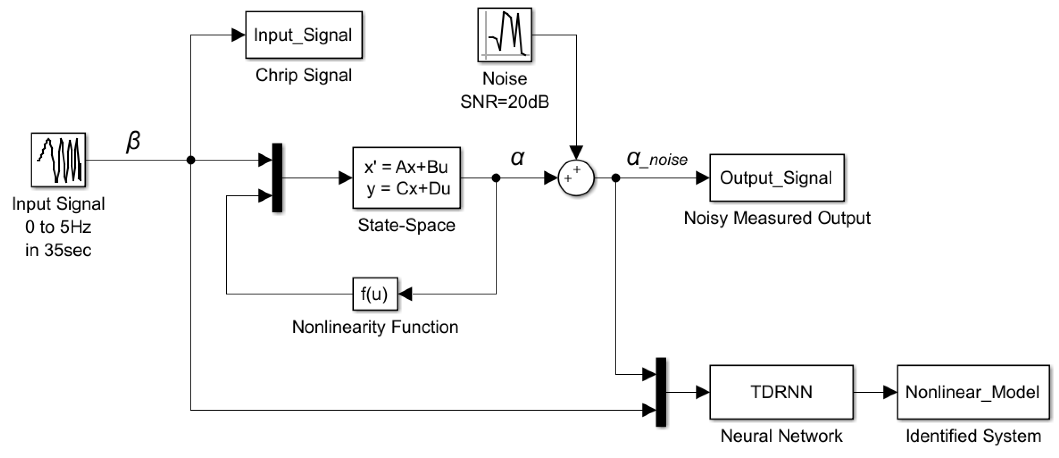
The TDRNN consists of input, hidden, and output layers. The hidden layer contains the input and feedback nodes and nonlinear and linear neurons. A feedback connection is present in the hidden layer. The time-delay memory elements ($Z^{-1}$) are used to store previous values of the input signal and output (feedback) signal. $W$ denotes the weight of the neuron. The weights ($W$) can be adjusted during the training process until accuracy of the neural network meets requirements. $\mathrm{b}$ represents the bias of the neuron. $f_1$ and $f_2$ are transfer functions. The structure of the TDRNN is shown in Figure 1.

The input–output relationship of the TDRNN is written as follows:

$$y\left(t\right)=f\left(y\left(t-1\right),y\left(t-2\right),\dots ,y\left(t-p\right),x\left(t-1\right),\dots ,x\left(t-q\right)\right)$$

(1)

where $x\left(t\right)$ is the input value at $t$ moment, $y\left(t\right)$ is the output value at $t$ moment. The output signal $y\left(t\right)$ is regressed on previous values of the output signal ($y\left(t-1\right),y\left(t-2\right),\dots ,y\left(t-p\right)$) and previous values of an independent (exogenous) input signal ($x\left(t-1\right),\dots ,x\left(t-q\right)$).

The mean squared error (MSE) of training data is used to evaluate performance of the proposed TDRNN, which is defined as:

$$MSE={\displaystyle \sum }_{t=1}^N{\left(\widehat{y}\left(t\right)-y\left(t\right)\right)}^2/N$$

(2)

where $\widehat{y}\left(t\right)$ is the estimated value of the TDRNN, $y\left(t\right)$ is the real value of the nonlinear aeroelastic system, which is obtained from the numerical simulation or wind-tunnel experiment. $N$ is the number of the calculated data values.

Taking control surface flap deflection ($\beta$) as the system input signal and pitch angle ($\alpha$) as the only considered output signal, the aeroelastic system is a single-input-single-output (SISO) system. The flowchart for neural network identification is shown in Figure 2. Measurement noise with an intensity of signal-to-noise ratio (SNR) = 20 dB is added to the output signal to simulate the actual environment. A TDRNN is used to approach the nonlinear aeroelastic system. The input and output data obtained from the simulation is divided into three parts. The first part is the training set (70%), which is used to compute the gradient and update network weights and biases. The second part is the validation set (15%), which is used to evaluate the network during the training process. The third part is the test set (15%), which is used to compare different models. After the network has been trained, it can be used to estimate the response of the nonlinear aeroelastic system.

3. Nonlinear Aeroelastic System Model

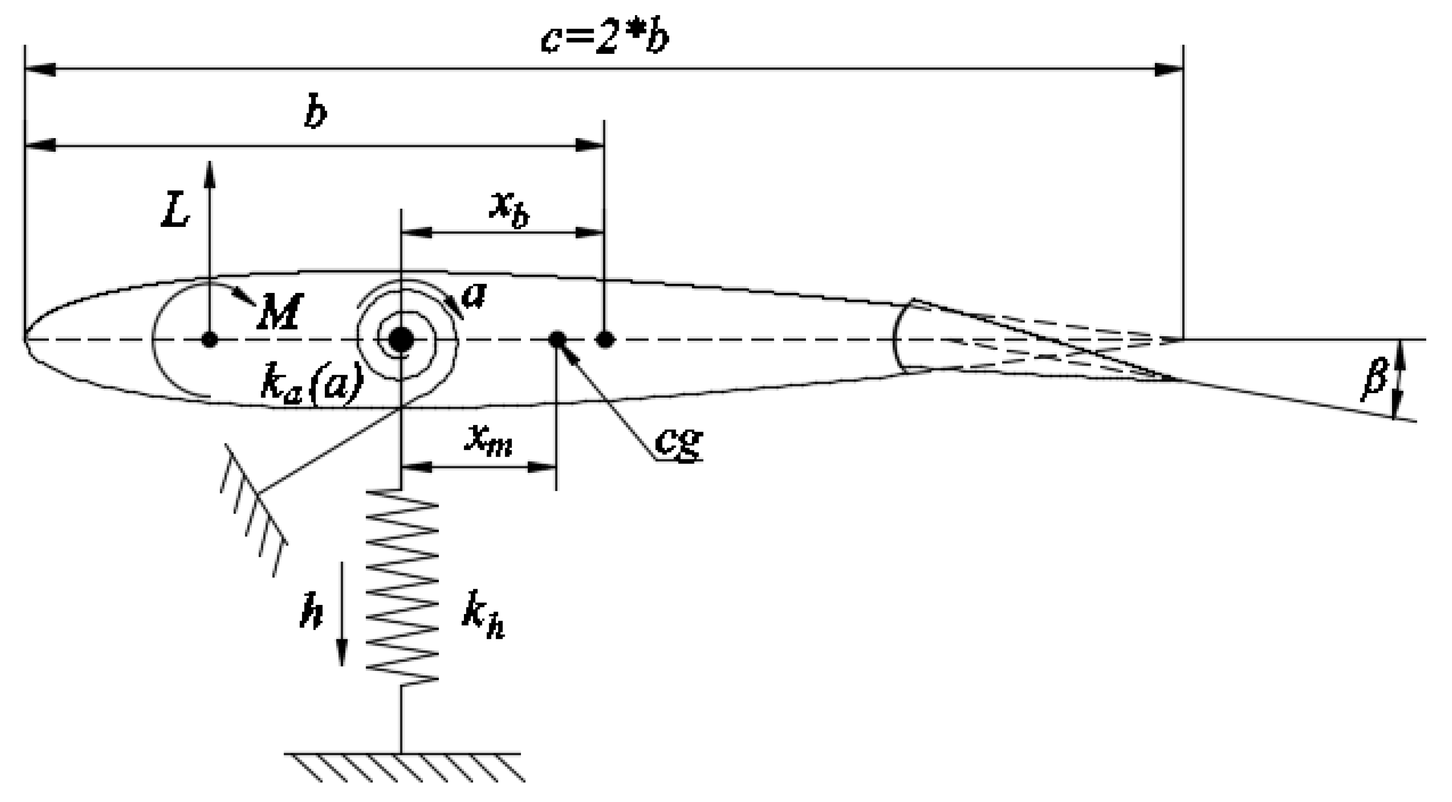
A typical two-dimensional wing section with a control surface is illustrated in Figure 3. This includes the plunge ($h$), the pitch ($\alpha$) of the main wing, and the flap ($\beta$) of the control surface.

Other parameters of the model are shown in

Table 1. Nonlinear aeroelastic system parameters.

Parameter	Value
$V$	6 m/s
$\rho$	1.225 kg/m3
$b$	0.135 m
$m$	12.387 kg
$x_m$	0.2466
$x_b$	−0.6
$I_{\alpha }$	0.065 kg·m2
$c_h$	27.43 kg/s
$c_{\alpha }$	0.180 kg·m2/s
$k_h$	2844.2 N/m
$k_{\alpha }$	2.82 Nm/rad
$c_{l\alpha }$	$2\pi$
$c_{l\beta }$	3.358
$c_{m\alpha }$	−0.628
$c_{m\beta }$	−0.635

[12]. Governing equations of motion for the structure of the nonlinear aeroelastic system are derived to be:

$$\left[\begin{array}{cc}m& m{x}_{m}b\\ m{x}_{m}b& I_a\end{array}\right]\left\{\begin{array}{c}\ddot{h}\\ \ddot{\alpha }\end{array}\right\}+\left[\begin{array}{cc}{c}_h& 0\\ 0& c_a\end{array}\right]\left\{\begin{array}{c}\dot{h}\\ \dot{\alpha }\end{array}\right\}+\left[\begin{array}{cc}{k}_h& 0\\ 0& k_a\end{array}\right]\left\{\begin{array}{c}h\\ \alpha \end{array}\right\}+\left[\begin{array}{c}0\\ M_{\alpha }\left(\alpha \right)-k_a\alpha \end{array}\right]=\left\{\begin{array}{c}-L\\ M_a\end{array}\right\}$$

(3)

Constants are defined as follows: $m$ is the mass of the wing section; $b$ is the semi-chord of the airfoil; $I_a$ is the moment of inertia about the elastic axis; $x_m$ is the non-dimensional distance between the mass center and elastic axis; $c_h$ and $c_a$ represent structural damping coefficients of the wing in plunge and pitch, respectively; and $k_h$ and $k_a$ are stiffness coefficients of the wing in plunge and pitch, respectively.

$L$ and $M_{\alpha }$ are the aerodynamic lift and moment, which can be defined as follows [19]:

$$L=\rho V^{2}b{c}_{l\alpha }\left[\alpha +\frac{\dot{h}}{V}+\left(\frac{1}{2}-x_b\right)b\frac{\dot{\alpha }}{V}\right]+\rho V^{2}b{c}_{l\beta }\beta$$

(4)

$$M_{\alpha }=\rho V^2{b}^2{c}_{m\alpha }\left[\alpha +\frac{\dot{h}}{V}+\left(\frac{1}{2}-x_b\right)b\frac{\dot{\alpha }}{V}\right]+\rho V^2{b}^2{c}_{m\beta }\beta$$

(5)

where $\rho$ is the free-stream density; $V$ is the inflow velocity; $c_{l\alpha }$ and $c_{m\alpha }$ are the lift and moment coefficient per angle of attack, respectively; $c_{l\beta }$ and $c_{m\beta }$ are the lift and moment coefficient per control surface deflection ($\beta$), respectively; $x_b$ is the non-dimensional distance between the mid-chord and the elastic axis; $\beta$ is the flap displacement of the control surface; and $M_{\alpha }\left(\alpha \right)$ is the moment-rotation relationship of pitch angle ($\alpha$).

Substituting Equations (4) and (5) into Equation (3), the following is obtained:

$$\begin{gathered} \left[\begin{array}{cc}m& m{x}_{m}b\\ m{x}_{m}b& I_a\end{array}\right]\left\{\begin{array}{c}\ddot{h}\\ \ddot{\alpha }\end{array}\right\}+\left[\begin{array}{cc}{c}_h+\rho Vb{c}_{l\alpha }& \rho V{b}^2{c}_{l\alpha }\left(\frac{1}{2}-x_b\right)\\ -\rho V{b}^2{c}_{m\alpha }& c_a-\rho V{b}^3{c}_{m\alpha }\left(\frac{1}{2}-x_b\right)\end{array}\right]\left\{\begin{array}{c}\dot{h}\\ \dot{\alpha }\end{array}\right\} \\ +\left[\begin{array}{cc}{k}_h& \rho V^{2}b{c}_{l\alpha }\\ 0& k_{\alpha }-\rho V^2{b}^2{c}_{m\alpha }\end{array}\right]\left\{\begin{array}{c}h\\ \alpha \end{array}\right\}+\left[\begin{array}{c}0\\ M_{\alpha }\left(\alpha \right)-k_{\alpha }\alpha \end{array}\right]=\left\{\begin{array}{c}-\rho V^{2}b{c}_{l\beta }\\ \rho V^2{b}^2{c}_{m\beta }\end{array}\right\}\beta \end{gathered}$$

(6)

Defining:

$$\begin{array}{l}M=\left[\begin{array}{cc}m& m{x}_{m}b\\ m{x}_{m}b& I_a\end{array}\right],\\ C=\left[\begin{array}{cc}{c}_h+\rho Vb{c}_{l\alpha }& \rho V{b}^2{c}_{l\alpha }\left(\frac{1}{2}-x_b\right)\\ -\rho V{b}^2{c}_{m\alpha }& c_a-\rho V{b}^3{c}_{m\alpha }\left(\frac{1}{2}-x_b\right)\end{array}\right],\\ K=\left[\begin{array}{cc}{k}_h& \rho V^{2}b{c}_{l\alpha }\\ 0& k_{\alpha }-\rho V^2{b}^2{c}_{m\alpha }\end{array}\right],\\ F_1=\left\{\begin{array}{c}-\rho V^{2}b{c}_{l\beta }\\ \rho V^2{b}^2{c}_{m\beta }\end{array}\right\},\\ F_2=\left[\begin{array}{c}0\\ 1\end{array}\right].\end{array}$$

Substituting $M,C,K,F_1,F_2$ into Equation (6), it may be expressed in a compact matrix form as:

$$M\left\{\begin{array}{c}\ddot{h}\\ \ddot{\alpha }\end{array}\right\}+C\left\{\begin{array}{c}\dot{h}\\ \dot{\alpha }\end{array}\right\}+K\left\{\begin{array}{c}h\\ \alpha \end{array}\right\}+F_2\left(M_{\alpha }\left(\alpha \right)-k_{\alpha }\alpha \right)=F_1\beta$$

(7)

The transformed equations of motions in the state space form become:

$$\dot{X}=AX+B_1\beta +B_2\left(k_{\alpha }\alpha -M_{\alpha }\left(\alpha \right)\right)$$

(8)

where:

• $X={\left[\begin{array}{ccc}h& \alpha & \begin{array}{cc}\dot{h}& \dot{\alpha }\end{array}\end{array}\right]}^T$,
• $A=\left[\begin{array}{cc}0& I\\ -M^{-1}K& -M^{-1}C\end{array}\right]$,
• $B_1=\left[\begin{array}{c}0\\ M^{-1}{F}_1\end{array}\right]$, and
• $B_2=\left\{\begin{array}{c}0\\ M^{-1}{F}_2\end{array}\right\}$.

The results of Equation (8) can be obtained by direct time marching integration.

4. Results and Discussion

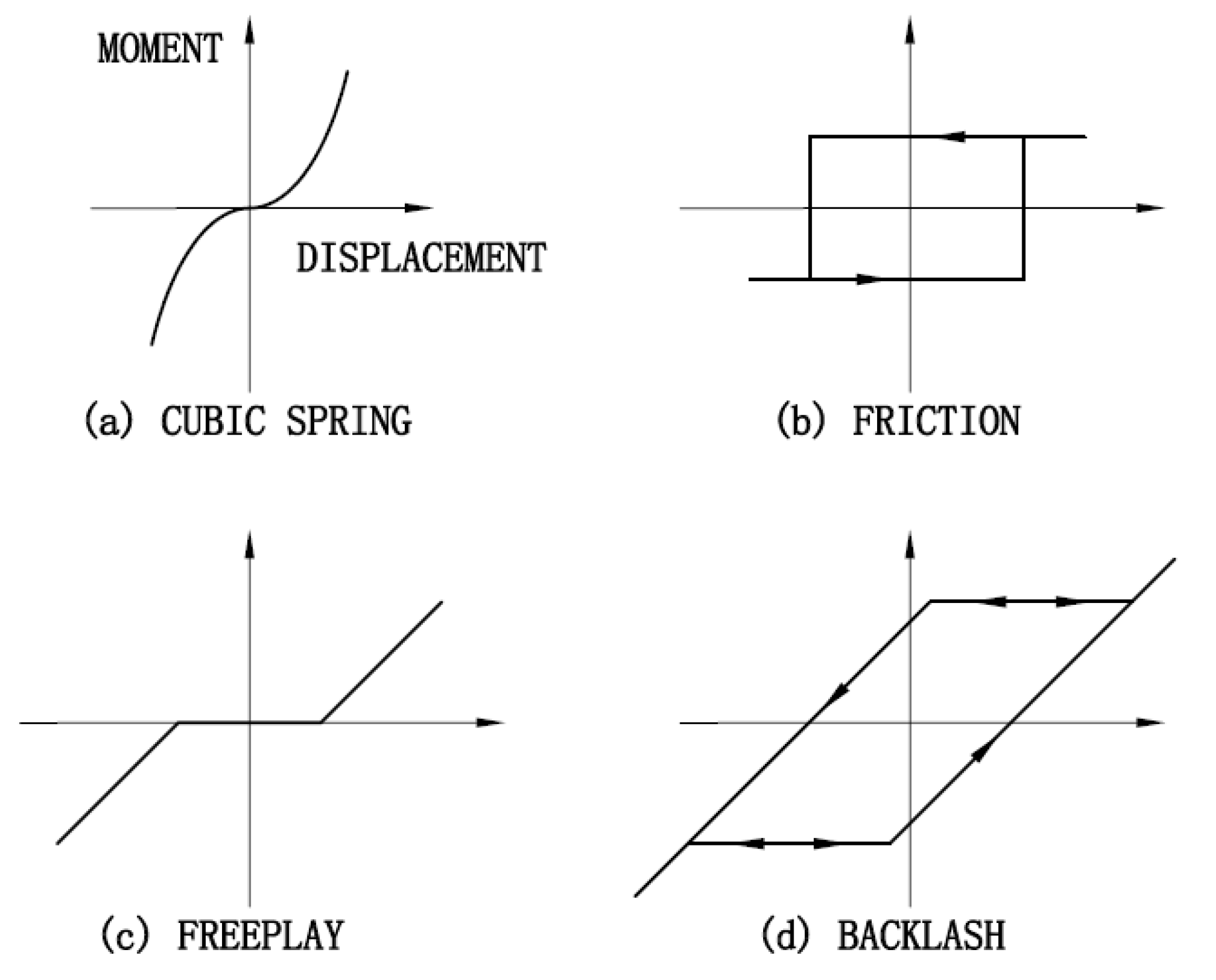
Real aeroelastic systems are often affected by a number of structural nonlinear factors, such as cubic-spring, friction, freeplay, backlash, hysteresis, time-delay, and saturation. Figure 4 shows the moment–displacement relationships of four types of structural nonlinear aeroelastic system.

In the present work, the cubic-spring and friction cases are carried out. These examples will illustrate the use of a neural network to identify the nonlinear aeroelastic system. The initial cases of the aeroelastic system are $h$ = 0, $\alpha$ = 0, $\dot{h}$ = 0, and $\dot{\alpha }$ = 0. Input signal of the system is a sine-sweep-chirp signal in the range of 0 to 5 Hz over 35 s. Time marching integration is used to produce response of the aeroelastic system.

4.1. Case 1: Cubic-Spring Nonlinearity

The first case of nonlinearity is the cubic-spring, the relationship between moment and displacement can be expressed as:

$$M_{\alpha }\left(\alpha \right)=k_{\alpha }\alpha +k_{\alpha 3}{a}^3$$

(9)

where $k_{\alpha 3}$ is cubic stiffness in the pitch direction, and $k_{\alpha 3}=$ 2.44.

Substituting Equation (9) into Equation (8), it is obtained that:

$$\dot{X}=AX+B_1\beta -B_2{k}_{\alpha 3}{a}^3$$

(10)

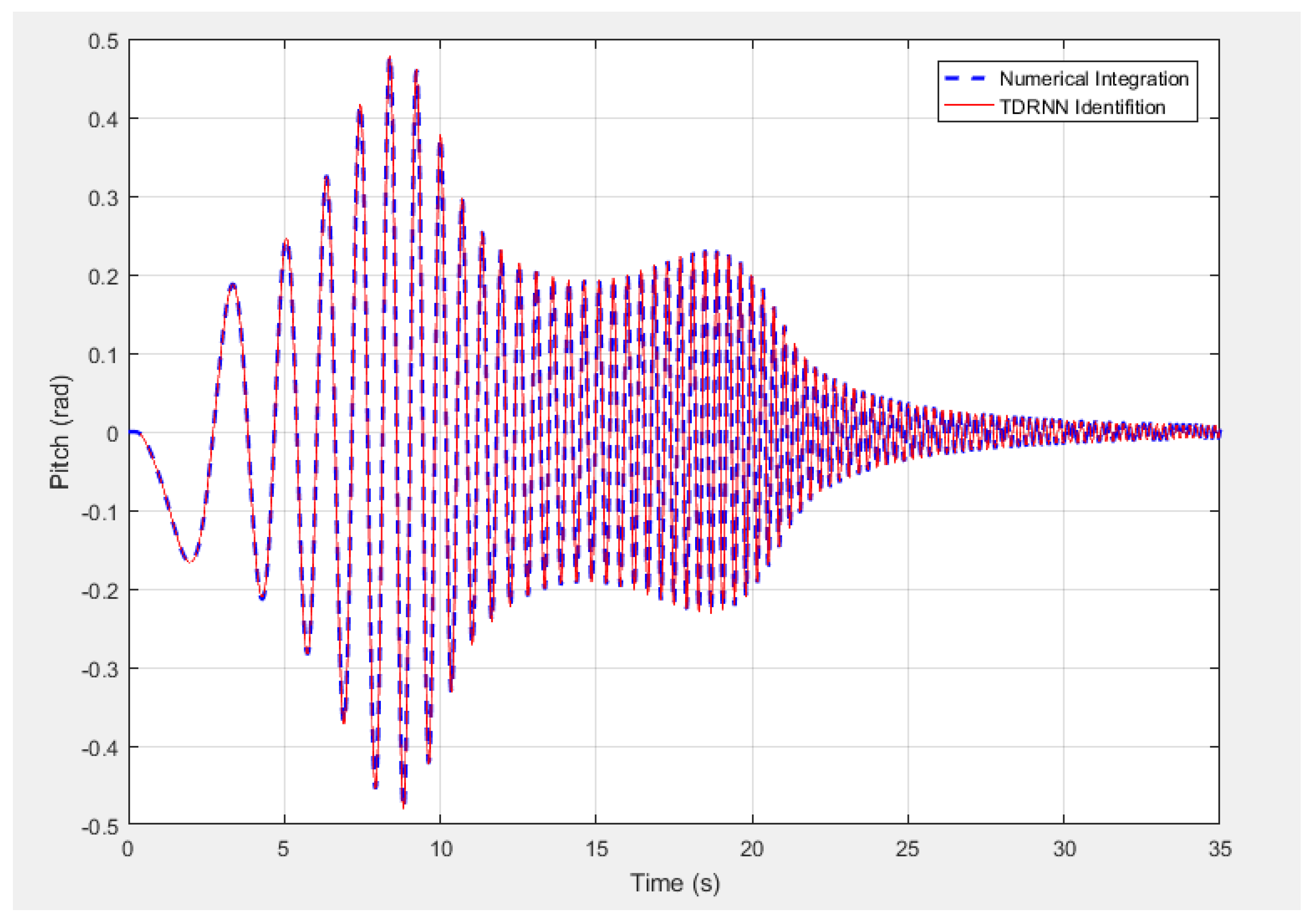
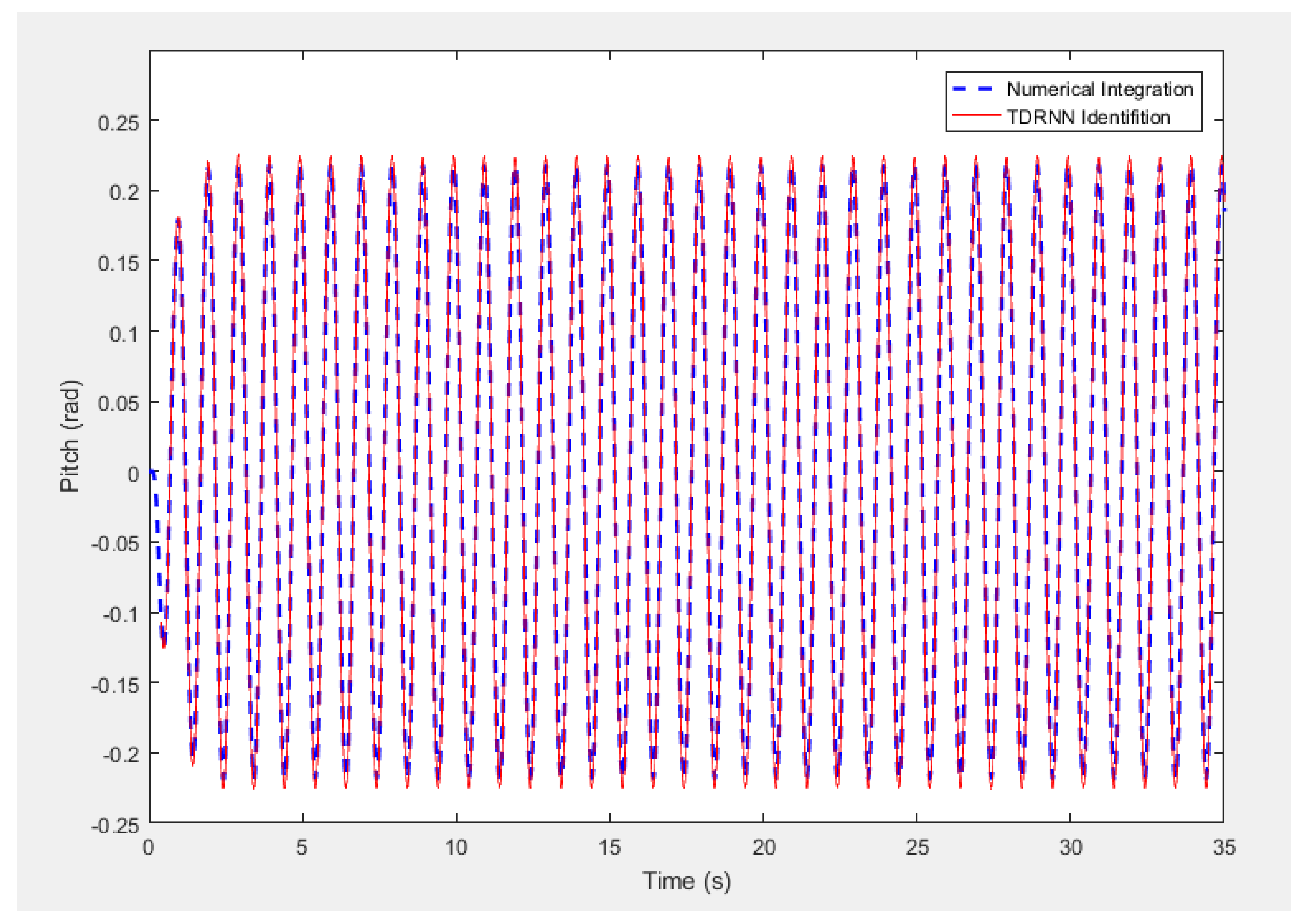
In this case, the standard Runge-Kutta algorithm is employed to produce theoretical results. Then, the neural network is trained by input and output data obtained by simulation. The chirp and sine input signals are used to verify the identified system. Responses of the system are calculated by time-marching-integration and the TDRNN net independently. Comparisons of estimation results with real results are shown in Figure 5 and Figure 6.

The dotted line shows the response of time-marching-integration and the solid line shows results of TDRNN. The two results are in very good agreement and it is hard to distinguish one from the other. The MSE of the chirp input signal is 4.3435 × 10⁻⁷ and the MSE of the sine input signal is 4.0733 × 10⁻⁷. The results indicate that the identified system approaches the real nonlinear aeroelastic system well.

Figure 7 shows a comparison of the input–output characteristic of the aeroelastic system with cubic-spring nonlinearity, when the excitation signal is sine function.

4.2. Case 2: Friction Nonlinearity

The second case of nonlinearity is friction. The Coulomb model is adopted as the friction force model in this paper. The moment-displacement relationship of the pitch angle is arbitrarily assumed to be:

$$M_{\alpha }\left(\alpha \right)=f_c·\mathrm{sgn}(\dot{\alpha )}$$

(11)

where $f_c$ is Coulomb’s friction force.

Substituting Equation (11) into Equation (8) yields:

$$\dot{X}=AX+B_1\beta +B_2(k_{\alpha }\alpha -f_c·\mathrm{sgn}(\dot{\alpha )})$$

(12)

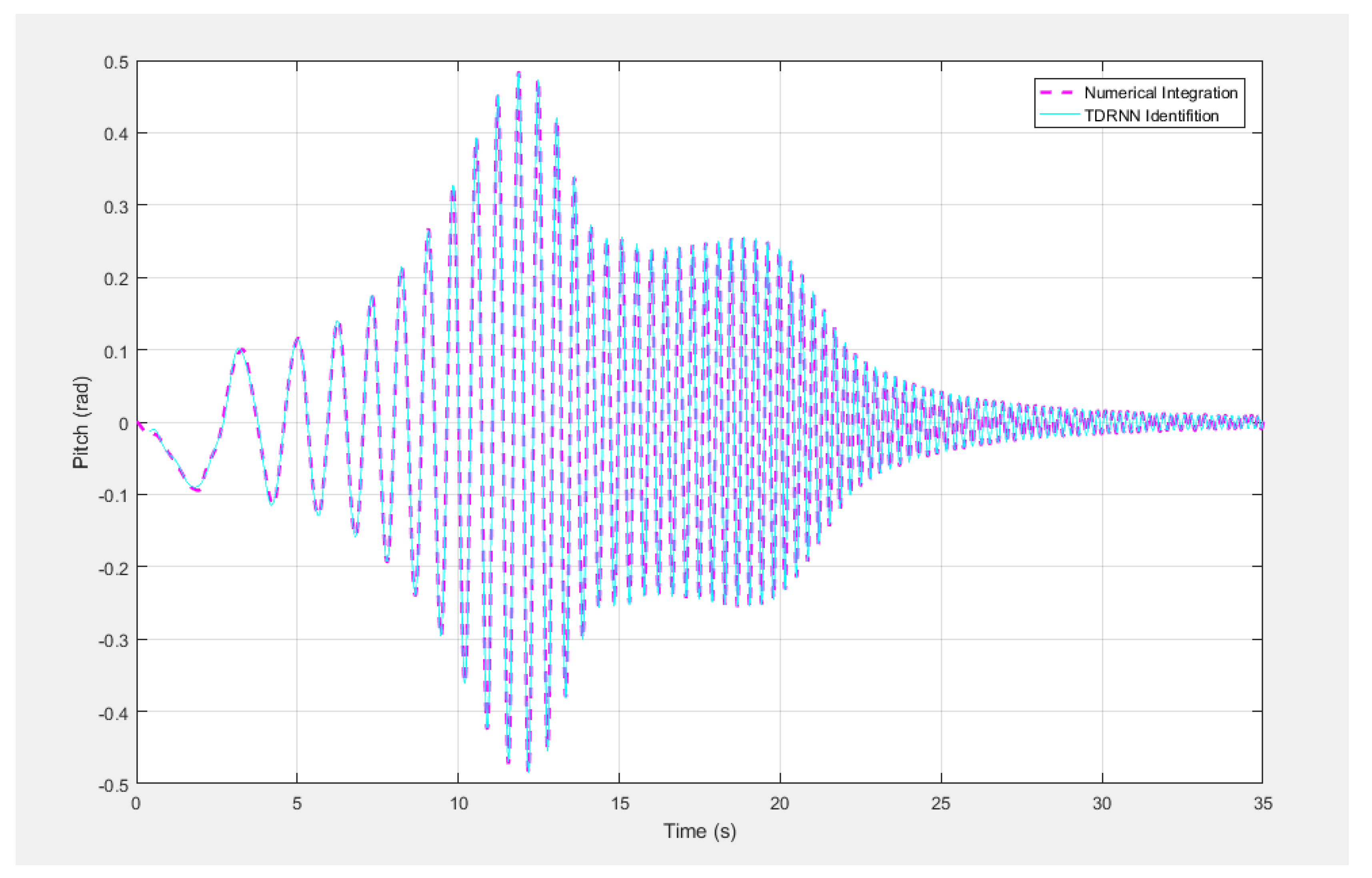
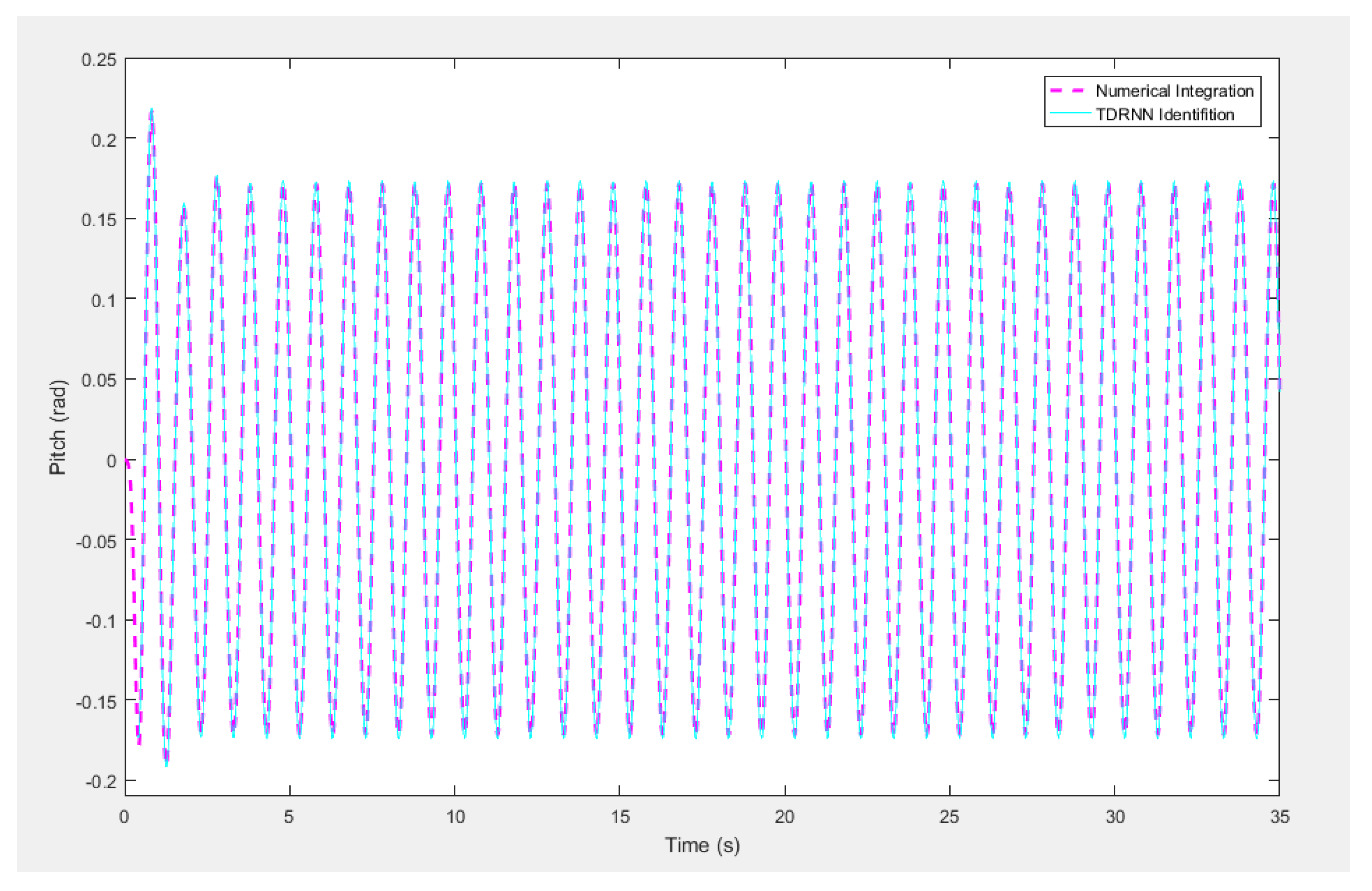
The chirp and sine input signals are also used to verify effectiveness of the neural network identification algorithm. Comparisons of estimation results with real results are illustrated in Figure 8 and Figure 9.

The dotted line shows the response of time-marching-integration and the solid line shows the results of TDRNN. The two results are similar and thus difficult to distinguish. The MSE of the chirp input signal is 2.6631 × 10⁻⁶ and the MSE of the sine input signal is 1.7472 × 10⁻⁶. Therefore, the identified system approaches the real nonlinear aeroelastic system effectively.

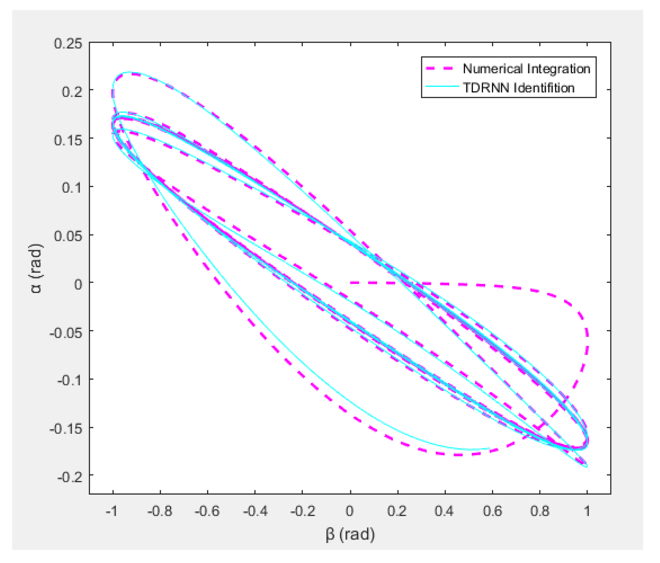
Figure 10 shows a comparison of the input–output characteristic of the aeroelastic system with friction nonlinearity, when the excitation signal is a sine function.

5. Conclusions

Traditional identification methods need to establish describing functions or approximate models of the system. Due to the complexity of the nonlinear aeroelastic system, it is hard to establish an accurate model of the system. The neural network identification method, which does not need to know the precise model of the system, is proposed to approach the nonlinear aeroelastic system. In this algorithm, a recurrent element is used to feedback results of output and a time-delay element is adopted to store previous values of the input and output signals. The TDRNN, which is trained by the simulation or experiment data, can be used to predict the response of the nonlinear aeroelastic system.

A typical three-degree-of-freedom wing section model is used to illustrate the methodology. Both cubic-spring and friction structural nonlinear aeroelastic systems are investigated in this study and responses calculated by direct time-marching-integration. A TDRNN is employed and trained by the simulated data. A frequency sweep input signal and a sinusoidal input signal are used to verify the identification model. The results show that the TDRNN can approach the accuracy of a nonlinear aeroelastic system and that the neural network identification method is a reliable and effective method.

References

- Theodorsen, T. General Theory of Aerodynamic Instability and the Mechanism of Flutter; NACA Rept. 496; NACA: Washington, DC, USA, 1935. [Google Scholar]
- Woolston, D.S.; Runyan, H.L.; Byrdsong, T.A. Some Effects of System Nonlinearities in the Problem of Aircraft Flutter; NACA TN 3539; NACA: Washington, DC, USA, 1955. [Google Scholar]
- Woolston, D.S.; Runyan, H.L.; Andrews, R.E. An Investigation of Effects of Certain Types of Structural Nonlinearities on Wing and Control Surface Flutter. J. Aeronaut. Sci. 1957, 24, 57–63. [Google Scholar] [CrossRef]
- Shen, S.F. An Approximate Analysis of Nonlinear Flutter Problems. J. Aerosp. Sci. 1958, 26, 25–32. [Google Scholar] [CrossRef]
- Breitbach, E. Effects of Structural Non-Linearities on Aircraft Vibration and Flutter; AGARD Rep. 665; AGARD: Reston, VA, USA, 1978. [Google Scholar]
- Laurenson, R.M.; Trn, R.M. Flutter Analysis of Missile Control Surfaces Containing Structural Nonlinearities. AIAA J. 1980, 18, 1245–1251. [Google Scholar] [CrossRef]
- Yang, Z.C.; Zhao, L.C. Analysis of Limit Cycle Flutter of an Airfoil in Incompressible Flow. J. Sound Vib. 1988, 123, 1–13. [Google Scholar] [CrossRef]
- Tang, D.M.; Dowell, E.H. Flutter and stall response of a helicopter blade with structural nonlinearity. J. Aircr. 1992, 29, 953–960. [Google Scholar] [CrossRef]
- Liu, L.; Dowell, E.H. Harmonic Balance Approach for an Airfoil with a Freeplay Control Surface. AIAA J. 2005, 43, 802–815. [Google Scholar] [CrossRef]
- Conner, M.D.; Tang, D.M.; Dowell, E.H.; Virgin, L.N. Nonlinear Behavior of a Typical Airfoil Section with Control Surface Freeplay A Numerical and Experimental Study. J. Fluids Struct. 1997, 11, 89–109. [Google Scholar] [CrossRef]
- Prazenica, R.J.; Lind, R.; Kurdila, A.J. Uncertainty Estimation from Volterra Kernels for Robust Flutter Analysis. J. Guid. Control Dyn. 2003, 26, 331–339. [Google Scholar] [CrossRef]
- Baldelli, D.H.; Lind, R.; Brenner, M. Nonlinear Aeroelastic/Aeroservoelastic Modeling by Block-Oriented Identification. J. Guid. Control Dyn. 2005, 28, 1056–1064. [Google Scholar] [CrossRef]
- Zeng, J.; Baldelli, D.H.; Brenner, M. Novel Nonlinear Hammerstein Model Identification Application to Nonlinear Aeroelastic/Aeroseroelastic System. J. Guid. Control Dyn. 2008, 31, 1677–1686. [Google Scholar] [CrossRef]
- Baldelli, D.H.; Zeng, J.; Lind, R.; Harris, C. Flutter Prediction Tool for Flight Test Based Aeroelastic Parameter Varying Models. J. Guid. Control Dyn. 2009, 32, 158–171. [Google Scholar] [CrossRef]
- Morino, H.; Obayashi, S. Nonlinear Aeroelastic Analysis of Control Surface with Freeplay Using Computational-Fluid-Dynamics-Based Reduced-Order Models. J. Aircr. 2015, 52, 569–583. [Google Scholar] [CrossRef]
- Mannarino, A.; Dowell, E.H. Reduced-Order Models for Computational-Fluid-Dynamics- Based Nonlinear Aeroelastic Problems. AIAA J. 2015, 53, 2671–2685. [Google Scholar] [CrossRef]
- Voitcu, O.; Wong, Y.S. Neural Network Approach for Nonlinear Aeroelastic Analysis. J. Guid. Control Dyn. 2003, 26, 99–105. [Google Scholar] [CrossRef]
- Dou, L.Q.; Ji, R.; Gao, J.Q. Identification of nonlinear aeroelastic system using fuzzy wavelet neural network. Neurocomputing 2016, 214, 935–943. [Google Scholar] [CrossRef]
- Fung, Y.C. An Introduction to the Theory of Aeroelasticity; Wiley: New York, NY, USA, 1955; pp. 207–215. [Google Scholar]
Figure 1.
Structure of the time-delay recurrent neural network (TDRNN).
Figure 2.
Flowchart for neural network identification. SNR: Signal-to-noise ratio.
Figure 3.
Typical two-dimensional wing section with control surface.
Figure 4.
Moment-displacement relationships of four types of structural nonlinear aeroelastic system.
Figure 5.
Response of chirp input signal.
Figure 6.
Response of sine input signal.
Figure 7.
Input–output characteristic of the aeroelastic system with cubic-spring nonlinearity.
Figure 8.
Figure 9.
Figure 10.
Input–output characteristic of the aeroelastic system with friction nonlinearity.