Infrared Image Super-Resolution Reconstruction Based on Quaternion Fractional Order Total Variation with Lp Quasinorm


1
School of Information and Communication Engineering, University of Electronic Science and Technology of China, Chengdu 610054, China
2
Chongqing College of Electronic Engineering, Chongqing 401331, China
*
Author to whom correspondence should be addressed.
Appl. Sci. 2018, 8(10), 1864; https://doi.org/10.3390/app8101864
Submission received: 3 September 2018
/
Revised: 1 October 2018
/
Accepted: 2 October 2018
/
Published: 10 October 2018
(This article belongs to the Special Issue Machine Learning and Compressed Sensing in Image Reconstruction)
Abstract
:Featured Application
This paper proposes a new super-resolution reconstruction method for infrared images, which makes a contribution to the research in infrared image processing and image reconstruction.
Abstract
Owing to the limitations of the imaging principle as well as the properties of imaging systems, infrared images often have some drawbacks, including low resolution, a lack of detail, and indistinct edges. Therefore, it is essential to improve infrared image quality. Considering the information of neighbors, a description of sparse edges, and by avoiding staircase artifacts, a new super-resolution reconstruction (SRR) method is proposed for infrared images, which is based on fractional order total variation (FTV) with quaternion total variation and the quasinorm. Our proposed method improves the sparsity exploitation of FTV, and efficiently preserves image structures. Furthermore, we adopt the plug-and-play alternating direction method of multipliers (ADMM) and the fast Fourier transform (FFT) theory for the proposed method to improve the efficiency and robustness of our algorithm; in addition, an accelerated step is adopted. Our experimental results show that the proposed method leads to excellent performances in terms of an objective evaluation and the subjective visual effect.
1. Introduction
Because of the imaging principle and other properties of infrared imaging systems, infrared images have low resolution with unclear edges; consequently, infrared images are not suitable for many applications. Considering this, it is considerably important to improve the quality of infrared images. There are currently two approaches to improve the resolution of infrared images: hardware and software approaches. For example, one hardware approach involves increasing the number of pixels per unit area, while another hardware approach involves increasing the size of the imaging system chip. These aforementioned hardware methods are not only difficult to implement, but also incur significant costs; thus, in recent years, various software approaches have been developed for the super-resolution reconstruction (SRR) of infrared images.
The objective of these image SRR software approaches is to recover a high-resolution (HR) image using one or multiple low-resolution (LR) images. In general, the image SRR methods can be classified into three types, including interpolation-based [1], learning-based, and regularization-based methods. The interpolation-based methods involve the construction of an HR image by projecting LR images onto reference images. Ur and Gross [2] proposed a method based on a non-uniformity interpolation from a set of spatially shifted LR images by utilizing the generalized multichannel sampling theorem of Papoulis [3] and Brown [4]. Zhang et al. developed an SR algorithm based on a bivariate rational fractal interpolation model, which achieved competitive performance with finer detail and sharper edges [5]. However, in methods based on interpolation, the optimality of the entire reconstruction algorithm is not guaranteed. In recent years, learning-based SRR has become a hot topic for research; in learning-based methods, the relationship between HR and LR images is obtained by learning the training samples and reconstructing the HR images based on the obtained relationship. In another study, Freeman et al. obtained the relationship between HR and LR image blocks using the Markov random field [6]. Donoho proposed the concept of sparse representation, which is a new method of signal representation [7]. Yang et al. proposed a super-resolution (SR) method based on this sparse representation [8,9]. Rajput et al. proposed an SR model based on the iterative sparsity and locality-constrained representation [10]; Huang et al. proposed a method which utilized an effective way to transform the large nonlinear feature space of LR images into a group of linear subspaces with mixture prior models in the training phase [11]. Though learning-based methods can achieve an excellent image visual effect, their high computational complexity limits its application. In contrast, methods based on regularization can capture the primary information and intrinsic geometry of an image with a small number of coefficients. In general, methods based on an integer-order partial differential equation (PDE) have obtained good results for image reconstruction; among these methods, a well-known method is total variation (TV) regularization [12,13], which not only eliminates noise, but also preserves the edges of the image well. However, first-order TV assumes images to be piece-wise constant, which introduces staircase artifacts; to address this limitation, several high-order variational methods have been proposed [14,15,16,17,18,19]. For example, Lysaker, Lundervold, and Tai first replaced the first-order TV by a second-order TV [20]. In addition, Chan, Esedoglu, and Park proposed the fourth-order TV combined with the Chambolle duality method to solve the issue of staircase artifacts [15]. Bredies, Kunisch, and Pock proposed total generalized variation (TGV) based on the combination of TV regularization with higher-order derivatives [21]; although these improved methods can alleviate the staircase artifacts, they might lead to “spots” effects on the processed image. In order to balance the staircase artifacts and “spots” effects, Zhang and Wei proposed a method based on the fractional-order gradient; in particular, in their method, they replaced the integer-order gradient with a fractional-order gradient [22]. Their research shows that using a fractional differential operator with 0 < v < 1 order to process the image not only appropriately processes the noise and edge information, but also enhances the texture and preserves the information related to the smooth region of the image. In fact, for noisy images, the conventional super-resolution way is to denoise the image as a pre-processing step and then super-resolve the de-noised image. Some new methods have been proposed [23,24,25], such as the median filter transform (MFT) with parallelogram shaped windows [23], which could be effectively used to integrate SR and image denoising to provide improved results in comparison to the conventional way.
In the case of SRR, another primary problem that needs to be addressed is the blocking artifact. To reduce the blocking artifact in a reconstructed image, Ren et al. proposed a fractional TV image SRR method [26,27]; their method involves using three parts: the integer-order TV item, the fractional-order TV (FTV) item, and the data fidelity item. The integer-order TV item can maintain the discontinuity and structure of the image, while the FTV item can suitably handle non-local information, such as the texture of the image. Thus, their method can slightly reduce the staircase artifacts in an image. To overcome the insufficiency of dealing with detail and texture information in the typical TV approach, Chen, Zhang, and Li proposed a two-dimensional (2D) compressive sensing sparse method for image reconstruction [28]. Their method introduces the FTV regularization term. In addition, to achieve elastic sparse representation, the discrete wavelet and curvelet transform regularization terms are combined into the cost function. Furthermore, Zachevsky and Zeevi proposed an SRR method based on the PDE of fractional Brownian motion to enhance the random texture information in an image [29]; this method is global and does not require image patches. Fractional Brownian motion is a stochastic process with self-similarity, which can significantly characterize natural texture information; consequently, it can effectively enhance the texture information of an image while enlarging it. Recently, Laghrib et al. proposed a non-convex fractional order variational model for image super-resolution; the use of the non-convex data fitting term can efficiently reduce complex noise such as impulse noise, while the fractional order regularization term can preserve image features like edges and texture much better [30].
In contrast, the TV method can only minimize horizontal and vertical gradients, reducing image noise in the horizontal and vertical directions, whereas the four-direction gradient regularization approach can reduce noise in the 45 and 135 directions, thereby improving the quality of image reconstruction [31,32]. Based on the four-direction TV (TV4) proposed by Sakurai et al. [31], Wu et al. presented a four-directional fractional-order TV (FTV4) [33], which applies the fractional-order difference operator to alleviate the staircase artifacts in TV4 and improve its denoising ability.
In the typical reconstruction method, the TV is based on the norm; however, in practice, many non-convex reconstruction methods outperform the norm sparse constrained reconstruction method. Chartrand first proposed the non-convex optimization problem with the quasinorm minimization (0 < p < 1) as the objective function [34,35]. Further, Sidky et al. replaced the norm with the norm in the minimization function and proposed a total p-variation (TpV) minimization algorithm [36]. Recently, Zhang et al. developed a reliable method which was performed in terms of the modulation transfer function, noise power spectrum, and noise equivalent quanta under different -norm priors in sparse-view X-ray CT reconstruction, and concluded that the best noise-resolution performance is achieved when p is between 0.8 and 1 [37]. Although using the norm leads to non-convex optimization problems, it might allow efficient image reconstruction with a few projection datasets for radiation dose reduction [38].
In this study, we explore the quaternion total variation and quasinorm relaxation to improve the sparsity exploitation of FTV; our proposed method is referred to as the quaternion fractional TV with quasinorm (), which is efficiently solved through plug-and-play alternating direction method of multipliers (ADMM) [39,40,41,42,43] in conjunction with non-convex p-shrinkage mapping. The novelty of our work is three-fold. First, the method is far less restrictive than the TV4 and FTV4 methods for infrared image reconstruction; it not only shows good performance in terms of detail preservation by incorporating high-order image derivatives, but also achieves accurate measurement of the sparsity potential from the regularity prior. Second, an efficient iterative algorithm is proposed to optimize the plug-and-play ADMM with a fast and stable convergence result. Third, fast and efficient closed-form solutions are investigated and derived for computationally complex sub-minimization problems using fast Fourier transforms (FFT).
The remainder of this paper is organized as follows. Section 2 briefly introduces the FTV method, TV4 method, and constrained TVp minimization method. Section 3 describes the proposed method as well as the fast plug-and-play ADMM algorithm for infrared image SRR. Then, in Section 4, our experiments and results are described. Finally, Section 5 and Section 6 present our discussion and conclusions, respectively.
2. Related Works
2.1. Fractional Total Variation
The v-order FTV is defined as follows:
where and represent the gradient operator of the image in the horizontal and vertical directions, respectively; these can be defined as follows [44]:
where and is the Gamma function.
The use of FTV can make the edges of an image more prominent while retaining the texture of the image. Moreover, because it handles pixels in the smooth region effectively, FTV is useful for avoiding staircase artifacts.
2.2. Four-Directional Total Variation
In 2011, Sakurai et al. proposed an extension of TV referred to as TV4 [31] in which both diagonal and back diagonal directional components are included in the typical TV model. TV4 can be defined as
Further, based on TV4, Liao et al. improved the boundary conditions and provided a complete mathematical proof for both anisotropic and isotropic cases [32]:
where , and and represent the anisotropic TV4 and isotropic TV4, respectively.
Compared with the typical TV, TV4 involves four-dimensional components of the spatial domain; these components consider the entire neighborhood information of every pixel, and thus, contain more structural information of the image.
2.3. Sparse Total Variation Based on Quasinorm
Compared with the norm, the quasinorm has one more degree of freedom; therefore, it can better characterize sparse gradient information. The contours of the anisotropic total variation (ATV) based on the quasinorm are shown in Figure 1, where the and norms are special cases of the norm. The norm is defined as , while the quasinorm is defined as . In Figure 1, white Gaussian noise is added to the image with a standard deviation of ; as can be seen from the figure, the intersection of the norm contours and fidelity term is not sparse, whereas the intersection of the norm contours and fidelity term is sparse, but is susceptible to noise pollution. In contrast, the contours of the quasinorm are more robust to noise.
3. Proposed Method
In this study, we propose an SRR method for infrared images based on the quaternion FTV with the quasinorm:
where is a circulant matrix that represents the convolution for the anti-aliasing filter. is a binary sampling matrix, where the rows are subsets of the identity matrix. Further, is an observation image, while represents the corresponding original image. represents the quaternion FTV with the quasinorm, which is defined as follows:
where represents the quasinorm. represents the convolution kernels along the horizontal, vertical, back diagonal, and diagonal directions, respectively; these are defined as follows:
where and ; in addition, is a function that returns A with its columns flipped in the left–right direction. The coefficient can be obtained as follows:
Thus, the proposed SRR method can be represented by
Furthermore, it can be rewritten as
To solve the model in the framework of the plug-and-play ADMM, an assistant variable is required to convert the unconstrained problem given by Equation (12) into the constrained problem:
Consequently, the corresponding augmented Lagrangian function is as follows:
where is the inner product of matrices and . is a Lagrange multiplier, and is a penalty parameter.
The minimizer of Equation (13) is the saddle point of , which can be found by solving the following sequence of sub-problems:
To solve the sub-problem of , let . Then, Equation (15) can be represented as follows
By setting the first-order derivative of in Equation (18) as zero, we have
Accordingly, the solution is
To solve the sub-problem , let . Then, Equation (16) can be transformed as follows:
Let ; then, Equation (21) can be rewritten as
By treating and as the original and noisy images, respectively, Equation (22) is the standard denoising model based on . Consequently, it can be replaced by using an image denoising algorithm to yield
where indicates the denoising process with the regularity parameter .
The proposed SRR algorithm is summarized in Algorithm 1.
| Algorithm 1 Super-resolution using the plug-and-play ADMM (alternating direction method of multipliers) |
| Initialize: Whiledo
|
In addition, based on the fast ADMM algorithm proposed by Goldstein et al. [45], we adopt the accelerated step , variables , and dual variables as
Compared with the accelerated step proposed by Nesterov et al. [46,47] that utilizes an accumulated history of the past iterates recursively, the abovementioned accelerated step only adopts the traditional projection-like step that is evaluated at an auxiliary point obtained from the previous two iterates and an explicit dynamically updated step size. After the accelerated step, the convergence rate increases from to .
This algorithm, which is referred to as SRR using the fast plug-and-play ADMM, is summarized in Algorithm 2.
Regarding the sub-problem , Equation (22) can be converted into the following constraint problem:
Accordingly, the augmented Lagrangian function is
where is the Lagrange multiplier, and is a penalty parameter. Furthermore, based on the ADMM algorithm, the sub-problem can be solved as follows:
| Algorithm 2 Super-resolution using the fast plug-and-play ADMM |
| Initialize: Whiledo
|
By employing the convolution theorem [48], the 2D Fourier transform of can be obtained as follows:
where the symbol ∘ represents component-wise multiplication.
By setting the first-order derivative of in Equation (30) as zero, we have
where is the conjugate map of .
Then, can be obtained as follows:
where represents the 2D inverse FFT operator; the division in the Equation (32) is component-wise as well. In addition, the symbol represents the matrix with all entries being 1.
The sub-problem is
Lastly, the Lagrange multiplier can be updated as
Similar to Algorithm 2, we introduce the acceleration step , variables , and dual variables :
In this manner, all the sub-problems of Equation (22) are solved independently. In all iterations, the sub-problem of is the most time-consuming problem. Considering the special structure of the differential matrices, we regard the differential operators as convolution operators. By introducing the convolution theorem, the sub-problem is skillfully solved in the frequency domain. The entire algorithm to solve Equation (22) is summarized in Algorithm 3.
| Algorithm 3 denoising using the fast ADMM |
| Initialize: Whiledo
|
4. Experiments and Results
4.1. Materials and Method
To verify the performance of the proposed method, six test images were employed from the infrared image databases of IRData (http://www.dgp.toronto.edu/~nmorris/data/IRData/) and LTIR (http://www.cvl.isy.liu.se/research/datasets/ltir/version1.0); these images are shown in Figure 2. Our experiments were performed on a PC with the Intel CPU 2.8 GHz and 8 GB RAM using MATLAB R2014a. Six different SRR methods were adopted for comparison, including the Bicubic method, the MFT method [23], the TV-based method [13], the TGV-based method [21], the TV4-based method [31], and the FTV4-based method [33]. Among the six methods, the Bicubic method was implemented by the function “imresize()” in the images toolbox of MATLAB; the MFT method used the scripts provided in [23]; other methods were taken by self-produced scripts according to [13,21,31,33].
For the objective evaluation, we calculated the peak signal-to-noise ratio (PSNR) and structural similarity (SSIM) [49]. These can be defined as follows:
where and represent the ground truth and reconstructed image, respectively. and are the mean values of and , respectively. Further, and are the variances in the and , respectively. is the covariance of and . The parameters and are set in a manner that ensures that the denominator of SSIM is a non-zero number. In this study, we set and .
Throughout all the experiments, we set the penalty parameters and of the quasinorm. The blur matrix in Equation (7) is set as a corresponding matrix to the blur kernel which is generated by the MATLAB built-in function “fspecial(‘gaussian’, 9, 1)”; is set as a K-fold downsampling operator which is generated by the MATLAB built-in function “downsample(X,K)”.
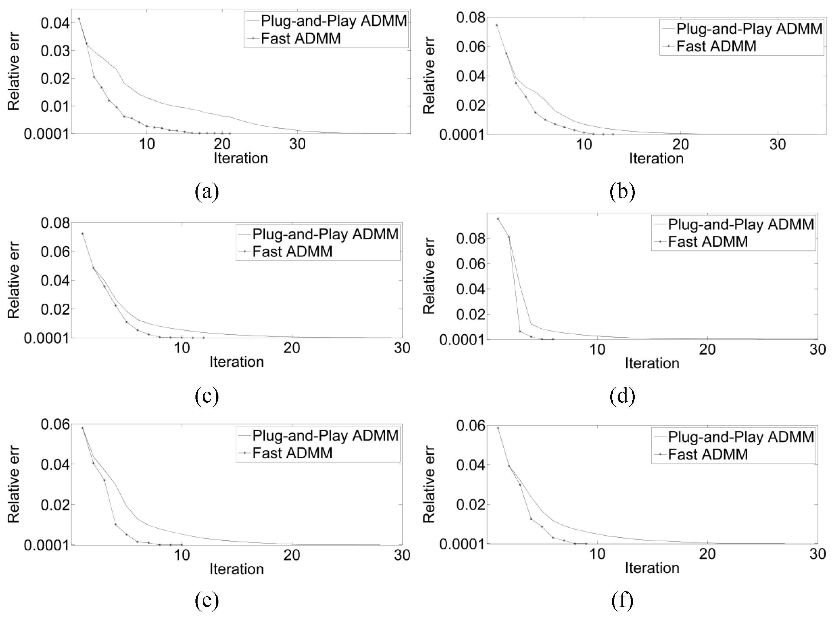
4.2. Comparison between Fast ADMM and Plug-and-Play ADMM
In order to verify the efficiency of the fast ADMM convergence, we adopted six images for comparison with the plug-and-play ADMM. The images were down-sampled by two-fold and white Gaussian noise was added to them. The standard deviation of the white Gaussian noise was set to 20.
4.3. Infrared Image SR Experiment Without Noise
In the experiment, the LR infrared images without noise were generated by applying the down-sampling operator (two-fold, three-fold, four-fold). To evaluate the performance objectively, PSNR and SSIM were calculated at various levels of the super-resolving operator (correspondingly, x2, x3, and x4) and are listed in Table 1.
In the SRR of the LR images with the two-fold downsampled operator, the PSNR of the method is the highest among the sets of results; however, the average PSNR of the six pictures is slightly higher than TGV, as well as being higher than the other methods. Furthermore, the SSIM of is good only in the image of birds; however, the overall SSIM is not as good as the TV4 and TGV methods, even though TV4 has a lower PSNR in four pictures. As the super-resolving operator increases, the results of are superior to the other algorithms. In terms of the computation time, the Bicubic method takes the shortest time, while MFT method takes the longest time, and the proposed method takes almost the same time as the TV4 and FTV4 methods.
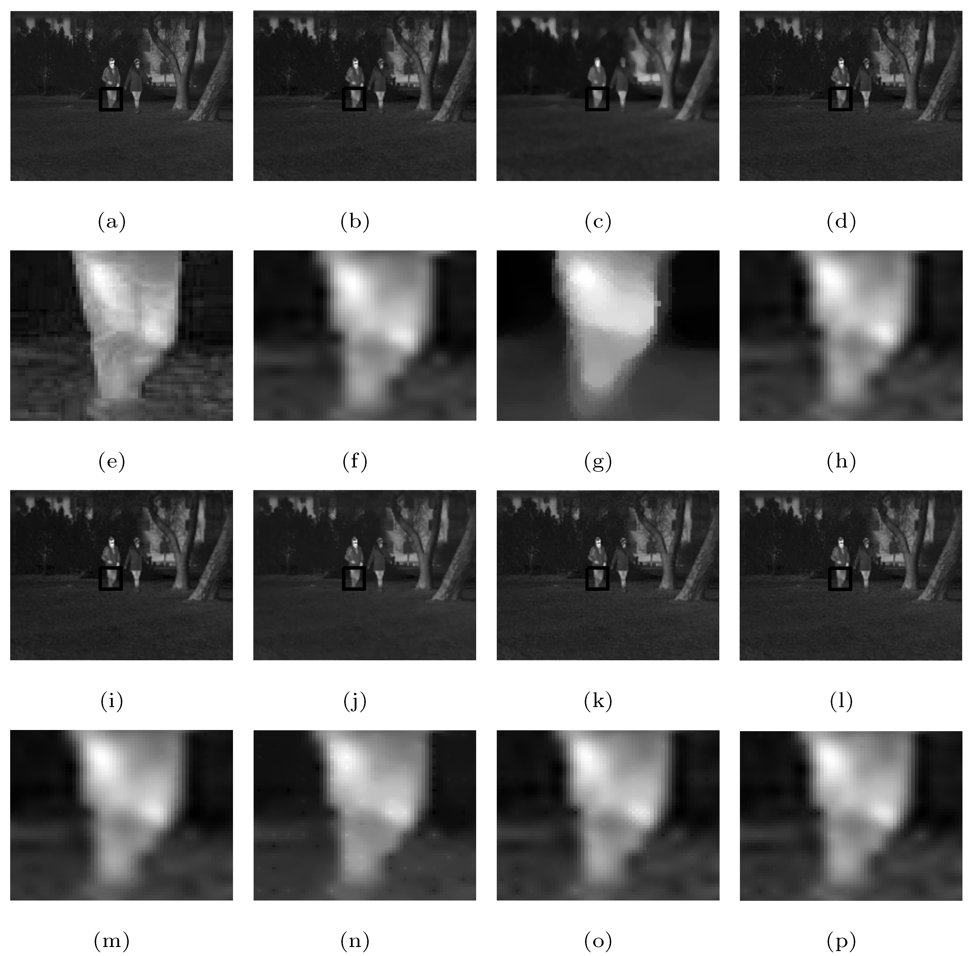
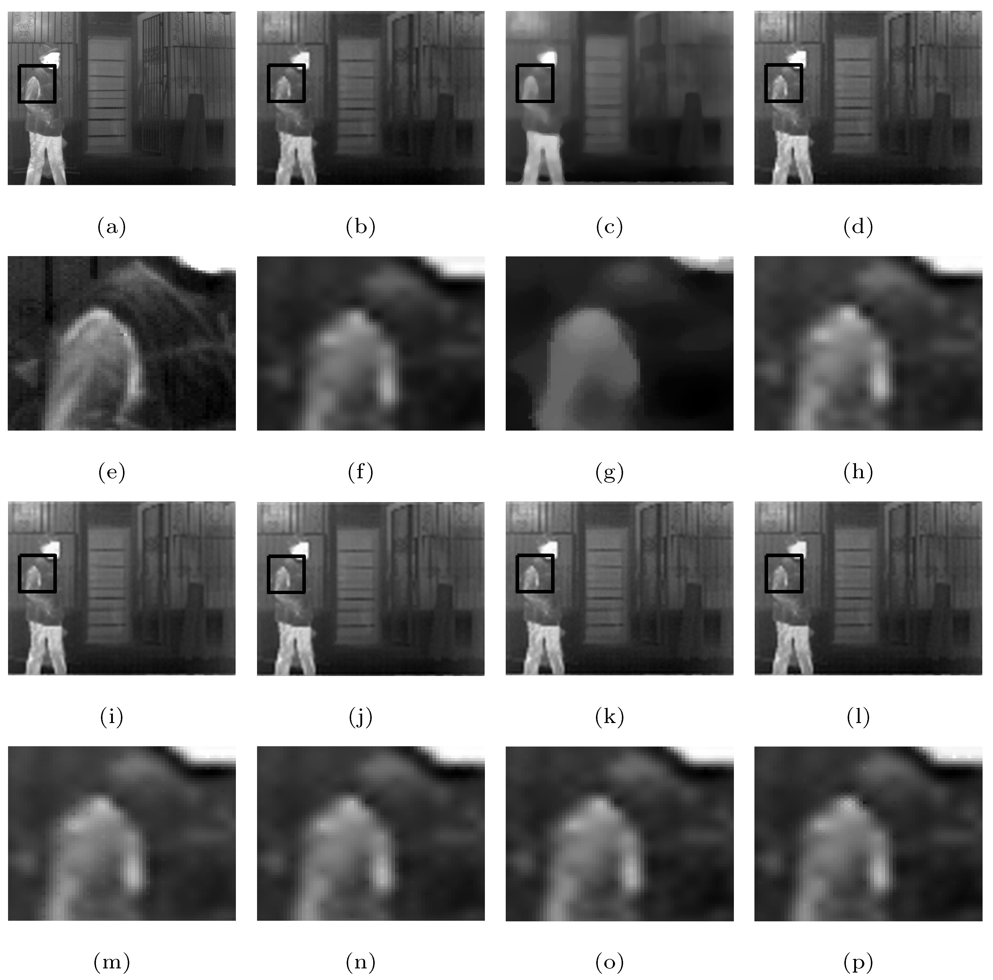
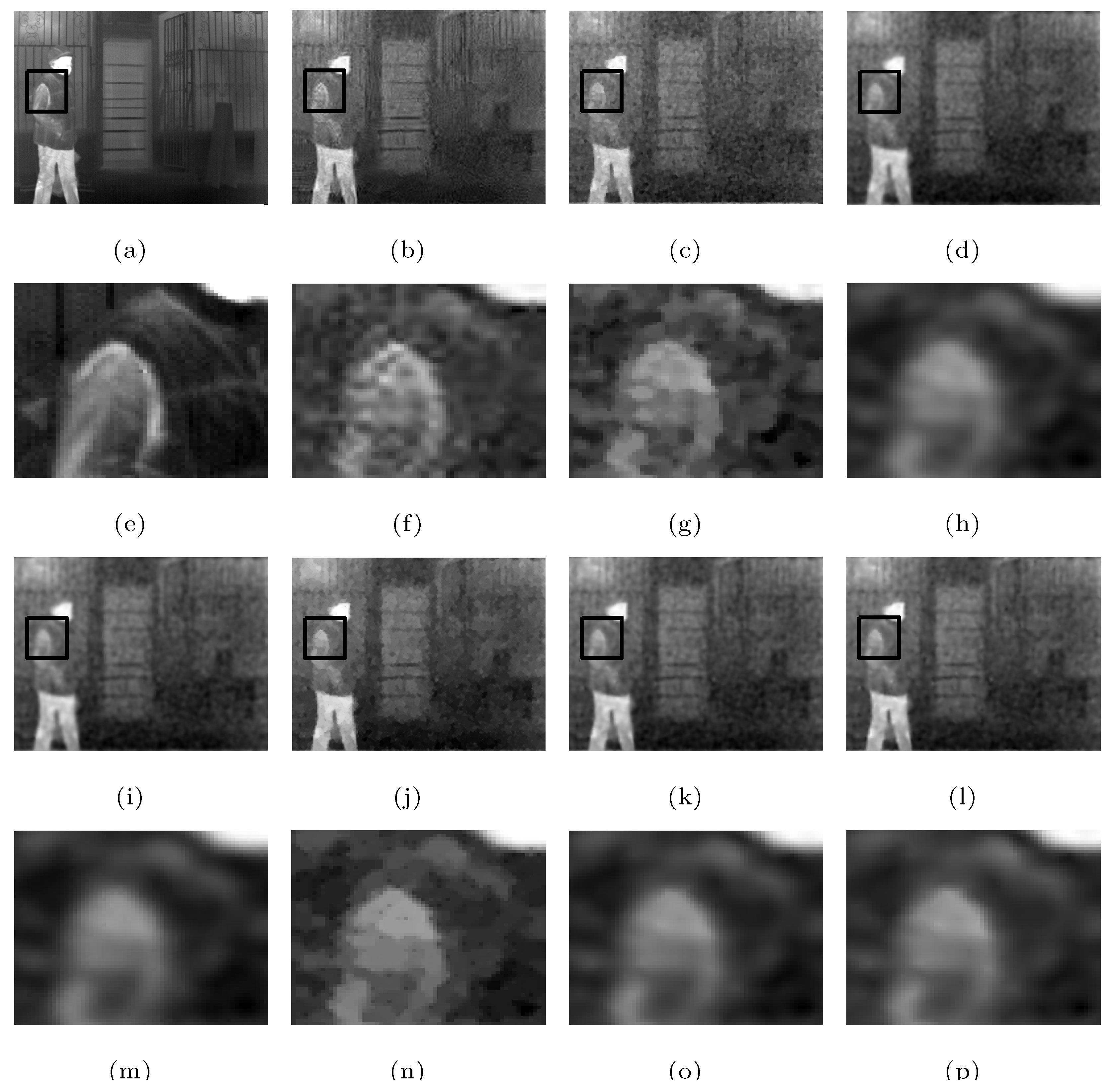
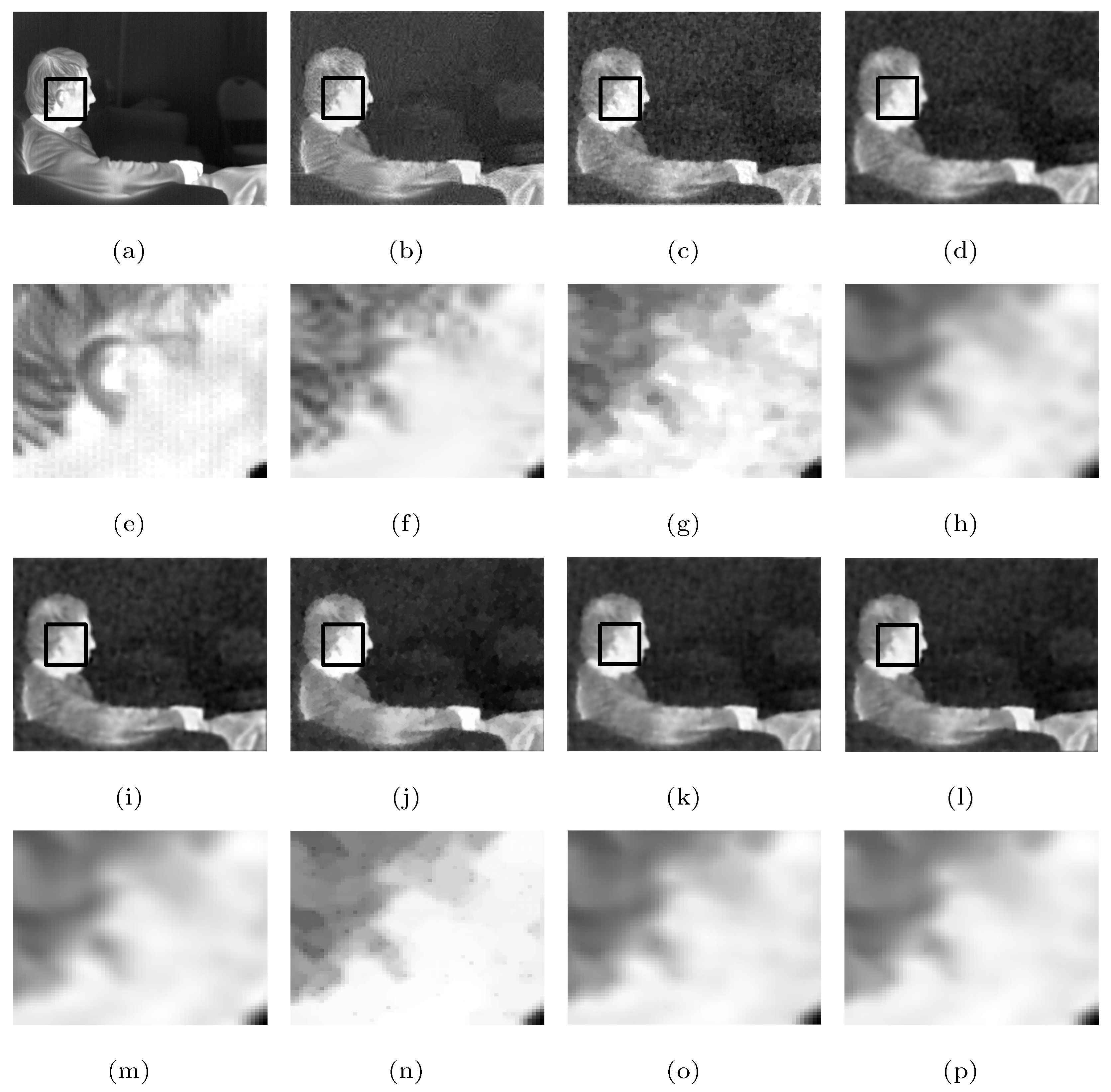
For a visual comparison, we used the LR infrared images of birds, passerby, and a figure, which are downsampled by four-fold in Figure 4.
Based on the results of the reconstruction of SR infrared images in Figure 5, Figure 6 and Figure 7, the edges of images reconstructed using the TV method are relatively clearer than the edges of images reconstructed using the Bicubic and MFT methods; however, staircase artifacts can be observed in the smooth regions of the images. The TGV, TV4, and FTV4 methods lead to improvements in terms of the staircase artifacts; however, many obvious “spots” remain in the bird and passerby images. In contrast, our proposed method performs better than the other four methods in terms of preserving image edges, as well as reducing staircase artifacts and “spots” effects.
4.4. Infrared Image Super-Resolution Experiment with Added White Gaussian Noise
In this experiment, the LR infrared images were generated by applying the two-fold down-sampling operator after which white Gaussian noise of different variance () was added. In order to perform a fair comparison under noise, a denoising pre-processing step was added to the Bicubic. To evaluate the performance of the various methods objectively, PSNR and SSIM were calculated at the x2 super-resolving operator; these results are listed in Table 2.
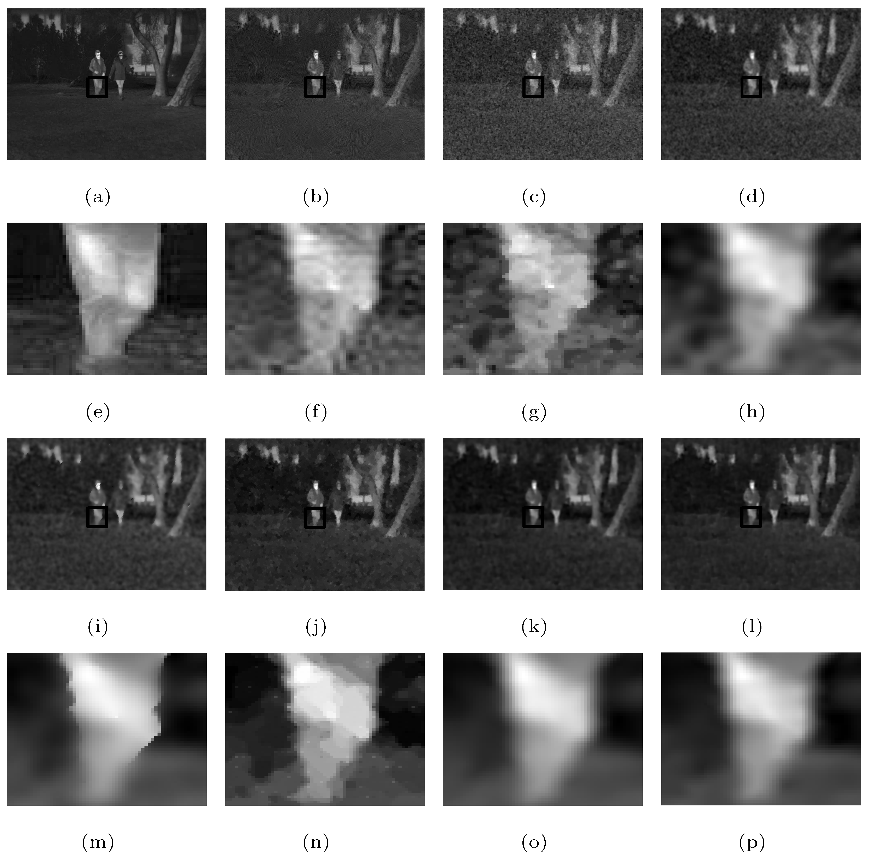
As is clear from Table 2, all the results of the TV-based method are poor. When , the reconstruction results of MFT, TGV and TV4 in the streets, building, passerby and figure images are slightly superior to the proposed method; however, when , their reconstruction results are worse than the proposed method. Furthermore, although the FTV4-based method has no obvious advantage in the SRR with added white Gaussian noise at any particular level, its average result is still superior to the other three methods and is only slightly inferior to the proposed method. In addition, the computation time of all methods becomes significantly longer with an increasing amount of added white Gaussian noise, and the Bicubic method still takes the shortest amount of time among all methods. The proposed method takes almost the same amount of time as the FTV4 method, and longer than the TV4 method. Therefore, considering the PSNR, SSIM, and computation time, the proposed method performs significantly better than the other six methods in most cases. In Figure 8, three infrared images, which have added white Gaussian noise () and were down-sampled by two-fold are shown as examples; the visual effects can still be observed in these images.
From the reconstructed images in Figure 9, Figure 10 and Figure 11, it can be observed that the images reconstructed using the Bicubic, MFT, and TV-based methods still contain considerable noise. In contrast, though the noise in the images reconstructed using the TGV-based method is reduced, some of the reconstructed images are significantly distorted compared with the original HR images. Furthermore, in the case of the TV4 reconstruction results, aside from image distortions, there are obvious “spots”; overall, the visual effect of reconstruction is poor. Finally, in terms of visual effects, the FTV4-based and proposed methods provide outstanding results; however, in terms of noise suppression, the results of the proposed method are superior.
5. Discussion
By extending to the quaternion TV and using the quasinorm constraint based on the FTV method, the proposed method fully utilizes image correlation in four directions and combines it with the quasinorm constraint to perform image reconstruction well, even in the presence of noise interference.
For the Bicubic and MFT methods, for both the noise-free and the added noise images, the reconstruction results are over-smoothed and the details are unclear.
Though the TV method preserves the edge and detail information of an image because of its piece-wise smooth processing, its results often include staircase artifacts. In contrast, because of the constraints of the image with the first-order and second-order gradients, the TGV-based method effectively reduces staircase artifacts; however, it also leads to over-smoothing and image distortion.
Without added white Gaussian noise, the TV4-based and FTV4-based methods show a “spots” effect in some images. Moreover, the TV4-based method has a similar “painting” effect under white Gaussian noisy conditions, which results in a large distortion relative to the original image. With white Gaussian noise, the visual effects of the FTV4 reconstruction are close to those of the proposed reconstruction; however, based on the experimental data analysis, the objective evaluation of the former is inferior to that of the reconstruction.
Furthermore, after introducing a fast ADMM algorithm, the number of ADMM iterations is significantly reduced, which improves the efficiency of the algorithm.
6. Conclusions
In this study, a fast SRR algorithm was proposed to improve the FTV by employing quaternion and quasinorm constraints. Because more neighbor observed information is considered in the proposed method, the SRR performance improves. Furthermore, by using the plug-and-play ADMM, the entire optimization problem is decoupled into several sub-problems that are considerably easier to solve. In our study, the differential operators are regarded as convolution operators; in this manner, the proposed model can be solved in the frequency domain using convolution theorem, thus avoiding large-scale matrix calculations.
We performed experiments on several infrared images; Our obtained results show that the proposed method outperforms the typical methods, including those based on TV, TGV, TV4, and FTV4.
Because the proposed model only focuses on the directions of FTV, it can be expanded to other models, such as the quaternion overlapping group sparse FTV model.
References
Author Contributions
X.L. wrote this manuscript. Y.C., Z.P., J.W. and Z.W. contributed to the writing, direction, and content, and revised the manuscript.
Funding
This research was funded by the National Natural Science Foundation of China (Nos. 61571096, 61775030, 61575038), the Scientific and Technological Research Program of Chongqing Municipal Education Commission (No. KJ1729409), the Natural Science Foundation of Fujian Province (No. 2015J01270), the Education and Scientific Research Foundation of Education Department of Fujian Province for Middle-aged and Young Teachers (No. JAT170352), the Chongqing Educational Science Planning Subject (No. 2015-ZJ-009), the Foundation of Fujian Province Great Teaching Reform (No. FBJG20180015), and the Open Foundation of Digital Signal and Image Processing Key Laboratory of Guangdong Province (No. 2017GDDSIPL-01).
Conflicts of Interest
The authors declare no conflict of interest.
References
- Zhou, F.; Yang, W.; Liao, Q. Interpolation-based image super-resolution using multisurface fitting. IEEE Trans. Image Process. 2012, 21, 3312–3318. [Google Scholar] [CrossRef] [PubMed]
- Ur, H.; Gross, D. Improved resolution from subpixel shifted pictures. CVGIP-Gr. Models Image Process. 1992, 54, 181–186. [Google Scholar] [CrossRef]
- Papoulis, A. Generalized sampling expansion. IEEE Trans. Circuits Syst. 1977, 24, 652–654. [Google Scholar] [CrossRef]
- Brown, J. Multi-channel sampling of low-pass signals. IEEE Trans. Circuits Syst. 1981, 28, 101–106. [Google Scholar] [CrossRef]
- Zhang, Y.; Fan, Q.; Bao, F.; Liu, Y.; Zhang, C. Single-Image Super-Resolution Based on Rational Fractal Interpolation. IEEE Trans. Image Process. 2018, 27, 3782–3797. [Google Scholar] [PubMed]
- Freeman, W.T.; Pasztor, E.C.; Carmichael, O.T. Learning low-level vision. Int. J. Comput. Vis. 2000, 40, 25–47. [Google Scholar] [CrossRef]
- Donoho, D.L. Compressed sensing. IEEE Trans. Inf. Theory 2006, 52, 1289–1306. [Google Scholar] [CrossRef]
- Yang, J.; Wright, J.; Huang, T.; Ma, Y. Image super-resolution as sparse representation of raw image patches. In Proceedings of the 2008 IEEE Conference on Computer Vision and Pattern Recognition, Anchorage, AK, USA, 23–28 June 2008; pp. 1–8. [Google Scholar]
- Yang, J.; Wright, J.; Huang, T.S.; Ma, Y. Image super-resolution via sparse representation. IEEE Trans. Image Process. 2010, 19, 2861–2873. [Google Scholar] [CrossRef] [PubMed]
- Rajput, S.S.; Arya, K.; Singh, V. Robust face super-resolution via iterative sparsity and locality-constrained representation. Inf. Sci. 2018, 463–464, 227–244. [Google Scholar] [CrossRef]
- Huang, Y.; Li, J.; Gao, X.; He, L.; Lu, W. Single Image Super-Resolution via Multiple Mixture Prior Models. IEEE Trans. Image Process. 2018, 27, 5904–5917. [Google Scholar] [CrossRef] [PubMed]
- Rudin, L.I.; Osher, S.; Fatemi, E. Nonlinear total variation based noise removal algorithms. Phys. D Nonlinear Phenom. 1992, 60, 259–268. [Google Scholar] [CrossRef]
- Marquina, A.; Osher, S.J. Image super-resolution by TV-regularization and Bregman iteration. J. Sci. Comput. 2008, 37, 367–382. [Google Scholar] [CrossRef]
- Chan, T.; Marquina, A.; Mulet, P. High-order total variation-based image restoration. SIAM J. Sci. Comput. 2000, 22, 503–516. [Google Scholar] [CrossRef]
- Chan, T.F.; Esedoglu, S.; Park, F. A fourth order dual method for staircase reduction in texture extraction and image restoration problems. In Proceedings of the 2010 17th IEEE International Conference on Image Processing (ICIP), Hong Kong, China, 26–29 September 2010; IEEE: Piscataway, NJ, USA, 2010; pp. 4137–4140. [Google Scholar]
- Liu, X.; Huang, L.; Guo, Z. Adaptive fourth-order partial differential equation filter for image denoising. Appl. Math. Lett. 2011, 24, 1282–1288. [Google Scholar] [CrossRef]
- Lysaker, M.; Tai, X.C. Iterative image restoration combining total variation minimization and a second-order functional. Int. J. Comput. Vis. 2006, 66, 5–18. [Google Scholar] [CrossRef]
- Li, F.; Shen, C.; Fan, J.; Shen, C. Image restoration combining a total variational filter and a fourth-order filter. J. Vis. Commun. Image Represent. 2007, 18, 322–330. [Google Scholar] [CrossRef]
- Chen, Y.; Wu, L.; Peng, Z.; Liu, X. Fast overlapping group sparsity total variation image denoising based on fast fourier transform and split bregman iterations. In Proceedings of the 2017 7th International Workshop on Computer Science and Engineering (WCSE 2017), Beijing, China, 25–27 June 2017; pp. 278–282. [Google Scholar]
- Lysaker, M.; Lundervold, A.; Tai, X.C. Noise removal using fourth-order partial differential equation with applications to medical magnetic resonance images in space and time. IEEE Trans. Image Process. 2003, 12, 1579–1590. [Google Scholar] [CrossRef] [PubMed] [Green Version]
- Bredies, K.; Kunisch, K.; Pock, T. Total generalized variation. SIAM J. Imaging Sci. 2010, 3, 492–526. [Google Scholar] [CrossRef]
- Jun, Z.; Zhihui, W. A class of fractional-order multi-scale variational models and alternating projection algorithm for image denoising. Appl. Math. Model. 2011, 35, 2516–2528. [Google Scholar] [CrossRef]
- Lopez-Rubio, E. Superresolution from a Single Noisy Image by the Median Filter Transform. SIAM J. Imaging Sci. 2016, 9, 82–115. [Google Scholar] [CrossRef]
- Qiu, F.; Xu, Y.; Wang, C.; Yang, Y. Noisy image super-resolution with sparse mixing estimators. In Proceedings of the 2011 4th International Congress on Image and Signal Processing (CISP), Shanghai, China, 15–17 October 2011; IEEE: Piscataway, NJ, USA, 2011; Volume 2, pp. 1081–1085. [Google Scholar]
- Singh, A.; Porikli, F.; Ahuja, N. Super-resolving noisy images. In Proceedings of the IEEE Conference on Computer Vision and Pattern Recognition, Columbus, OH, USA, 23–28 June 2014; pp. 2846–2853. [Google Scholar]
- Ren, Z.; He, C.; Zhang, Q. Fractional order total variation regularization for image super-resolution. Signal Process. 2013, 93, 2408–2421. [Google Scholar] [CrossRef]
- Ren, Z.; He, C.; Li, M. Fractional-order bidirectional diffusion for image up-sampling. J. Electron. Imaging 2012, 21, 023006. [Google Scholar] [CrossRef]
- Chen, G.; Zhang, J.; Li, D. Fractional-order total variation combined with sparsifying transforms for compressive sensing sparse image reconstruction. J. Vis. Commun. Image Represent. 2016, 38, 407–422. [Google Scholar] [CrossRef]
- Zachevsky, I.; Zeevi, Y.Y. Single-image superresolution of natural stochastic textures based on fractional Brownian motion. IEEE Trans. Image Process. 2014, 23, 2096–2108. [Google Scholar] [CrossRef] [PubMed]
- Laghrib, A.; Ben-loghfyry, A.; Hadri, A.; Hakim, A. A nonconvex fractional order variational model for multi-frame image super-resolution. Signal Proce. Image Commun. 2018, 67, 1–11. [Google Scholar] [CrossRef]
- Sakurai, M.; Kiriyama, S.; Goto, T.; Hirano, S. Fast algorithm for total variation minimization. In Proceedings of the 2011 18th IEEE International Conference on Image Processing (ICIP), Brussels, Belgium, 11–14 September 2011; IEEE: Piscataway, NJ, USA, 2011; pp. 1461–1464. [Google Scholar]
- Liao, F.; Coatrieux, J.L.; Wu, J.; Shu, H. A new fast algorithm for constrained four-directional total variation image denoising problem. Math. Probl. Eng. 2015, 2015, 815132. [Google Scholar] [CrossRef]
- Wu, L.; Chen, Y.; Jin, J.; Du, H.; Qiu, B. Four-directional fractional-order total variation regularization for image denoising. J. Electron. Imaging 2017, 26, 053003. [Google Scholar] [CrossRef]
- Chartrand, R. Exact reconstruction of sparse signals via nonconvex minimization. IEEE Signal Process. Lett. 2007, 14, 707–710. [Google Scholar] [CrossRef]
- Chartrand, R. Shrinkage mappings and their induced penalty functions. In Proceedings of the 2014 IEEE International Conference on Acoustics, Speech and Signal Processing (ICASSP), Florence, Italy, 4–9 May 2014; IEEE: Piscataway, NJ, USA, 2014; pp. 1026–1029. [Google Scholar]
- Sidky, E.Y.; Chartrand, R.; Boone, J.M.; Pan, X. Constrained TpV Minimization for Enhanced Exploitation of Gradient Sparsity: Application to CT Image Reconstruction. IEEE J. Trans. Eng. Health Med. 2014, 2, 1–18. [Google Scholar] [CrossRef] [PubMed]
- Zhang, L.; Zhao, H.; Ma, W.; Jiang, J.; Zhang, L.; Li, J.; Gao, F.; Zhou, Z. Resolution and noise performance of sparse view X-ray CT reconstruction via Lp-norm regularization. Phys. Med. 2018, 52, 72–80. [Google Scholar] [CrossRef] [PubMed]
- Cai, A.; Wang, L.; Yan, B.; Li, L.; Zhang, H.; Hu, G. Efficient TpV minimization for circular, cone-beam computed tomography reconstruction via non-convex optimization. Comput. Med. Imaging Gr. 2015, 45, 1–10. [Google Scholar] [CrossRef] [PubMed]
- Brifman, A.; Romano, Y.; Elad, M. Turning a denoiser into a super-resolver using plug and play priors. In Proceedings of the 2016 IEEE International Conference on Image Processing (ICIP), Phoenix, Arizona, 25–28 September 2016; IEEE: Piscataway, NJ, USA, 2016; pp. 1404–1408. [Google Scholar]
- Sreehari, S.; Venkatakrishnan, S.V.; Wohlberg, B.; Buzzard, G.T.; Drummy, L.F.; Simmons, J.P.; Bouman, C.A. Plug-and-play priors for bright field electron tomography and sparse interpolation. IEEE Trans. Comput. Imaging 2016, 2, 408–423. [Google Scholar] [CrossRef]
- Venkatakrishnan, S.V.; Bouman, C.A.; Wohlberg, B. Plug-and-play priors for model based reconstruction. In Proceedings of the Global Conference on Signal and Information Processing (GlobalSIP), Austin, TX, USA, 3–5 December 2013; IEEE: Piscataway, NJ, USA, 2013; pp. 945–948. [Google Scholar]
- Kamilov, U.S.; Mansour, H.; Wohlberg, B. A Plug-and-Play Priors Approach for Solving Nonlinear Imaging Inverse Problems. IEEE Signal Process. Lett. 2017, 24, 1872–1876. [Google Scholar] [CrossRef]
- Chan, S.H.; Wang, X.; Elgendy, O.A. Plug-and-Play ADMM for image restoration: Fixed-point convergence and applications. IEEE Trans. Comput. Imaging 2017, 3, 84–98. [Google Scholar] [CrossRef]
- Podlubny, I. FRactional Differential Equations: An Introduction to Fractional Derivatives, Fractional Differential Equations, to Methods of Their Solution and Some of Their Applications; Elsevier: Amsterdam, The Netherlands, 1998; Volume 198. [Google Scholar]
- Goldstein, T.; O’Donoghue, B.; Setzer, S.; Baraniuk, R. Fast alternating direction optimization methods. SIAM J. Imaging Sci. 2014, 7, 1588–1623. [Google Scholar] [CrossRef]
- Huang, B.; Ma, S.; Goldfarb, D. Accelerated linearized Bregman method. J. Sci. Comput. 2013, 54, 428–453. [Google Scholar] [CrossRef]
- Xie, Y.; Ke, Y.; Ma, C. The modified accelerated Bregman method for regularized basis pursuit problem. J. Inequal. Appl. 2014, 2014, 130. [Google Scholar] [CrossRef] [Green Version]
- Oppenheim, A.V.; Willsky, A.S.; Nawab, S.H. Signals and systems, vol. 2. Prentice-Hall Englewood Cliffs 1983, 6, 10. [Google Scholar]
- Wang, Z.; Bovik, A.C.; Sheikh, H.R.; Simoncelli, E.P. Image quality assessment: From error visibility to structural similarity. IEEE Trans. Image Process. 2004, 13, 600–612. [Google Scholar] [CrossRef] [PubMed]
Figure 1.
Feasible domain of : (a) , (b) and (c) .

Figure 2.
HR infrared images: (a) birds, (b) streets, (c) crossroads, (d) building, (e) passerby, and (f) figure.
Figure 2.
HR infrared images: (a) birds, (b) streets, (c) crossroads, (d) building, (e) passerby, and (f) figure.

Figure 3.
Comparisons of the convergence between the fast ADMM and plug-and-play ADMM. White Gaussian noise was added to the images: (a) birds, (b) streets, (c) crossroads, (d) buildings, (e) passerby, and (f) figure.
Figure 3.
Comparisons of the convergence between the fast ADMM and plug-and-play ADMM. White Gaussian noise was added to the images: (a) birds, (b) streets, (c) crossroads, (d) buildings, (e) passerby, and (f) figure.

Figure 4.
Low-resolution (LR) infrared images down-sampled four-fold without noise: (a) birds, (b) passerby, (c) figure.
Figure 4.
Low-resolution (LR) infrared images down-sampled four-fold without noise: (a) birds, (b) passerby, (c) figure.

Figure 5.
Super-resolution x4 results of the LR bird images without noise; (a–d,i–l) ground truth and the results of the Bicubic, MFT, TV, TGV, TV4, FTV4, and FTV4Lp methods, respectively; (e–h,m–p) enlarged details from the rectangles in (a–d,i–l), respectively.
Figure 5.
Super-resolution x4 results of the LR bird images without noise; (a–d,i–l) ground truth and the results of the Bicubic, MFT, TV, TGV, TV4, FTV4, and FTV4Lp methods, respectively; (e–h,m–p) enlarged details from the rectangles in (a–d,i–l), respectively.

Figure 6.
Super-resolution x4 results of the LR passerby images without noise; (a–d,i–l) ground truth and the results of the Bicubic, MFT, TV, TGV, TV4, FTV4, and FTV4Lp methods, respectively; (e–h,m–p) enlarged details from the rectangles in (a–d,i–l), respectively.
Figure 6.
Super-resolution x4 results of the LR passerby images without noise; (a–d,i–l) ground truth and the results of the Bicubic, MFT, TV, TGV, TV4, FTV4, and FTV4Lp methods, respectively; (e–h,m–p) enlarged details from the rectangles in (a–d,i–l), respectively.

Figure 7.
Super-resolution x4 results of the LR figure images without noise; (a–d,i–l) ground truth and the results of the Bicubic, MFT, TV, TGV, TV4, FTV4, and FTV4Lp methods, respectively; (e–h,m–p) enlarged details from the rectangles in (a–d,i–l), respectively.
Figure 7.
Super-resolution x4 results of the LR figure images without noise; (a–d,i–l) ground truth and the results of the Bicubic, MFT, TV, TGV, TV4, FTV4, and FTV4Lp methods, respectively; (e–h,m–p) enlarged details from the rectangles in (a–d,i–l), respectively.

Figure 8.
LR infrared images down-sampled by two-fold with added white Gaussian noise ( = 20): (a) birds, (b) passerby, (c) figure.
Figure 8.
LR infrared images down-sampled by two-fold with added white Gaussian noise ( = 20): (a) birds, (b) passerby, (c) figure.

Figure 9.
Super-resolution x2 results of the LR bird images with added white Gaussian noise ( = 20); (a–d,i–l) ground truth and the results of the Bicubic, MFT, TV, TGV, TV4, FTV4, and FTV4Lp methods, respectively; (e–h,m–p) enlarged details from the rectangles in (a–d,i–l), respectively.
Figure 9.
Super-resolution x2 results of the LR bird images with added white Gaussian noise ( = 20); (a–d,i–l) ground truth and the results of the Bicubic, MFT, TV, TGV, TV4, FTV4, and FTV4Lp methods, respectively; (e–h,m–p) enlarged details from the rectangles in (a–d,i–l), respectively.

Figure 10.
Super-resolution x2 results of the LR passerby images with added white Gaussian noise ( = 20); (a–d,i–l) ground truth and the results of the Bicubic, MFT, TV, TGV, TV4, FTV4 and FTV4Lp methods, respectively; (e–h,m–p) enlarged details from the rectangles in (a–d,i–l), respectively.
Figure 10.
Super-resolution x2 results of the LR passerby images with added white Gaussian noise ( = 20); (a–d,i–l) ground truth and the results of the Bicubic, MFT, TV, TGV, TV4, FTV4 and FTV4Lp methods, respectively; (e–h,m–p) enlarged details from the rectangles in (a–d,i–l), respectively.

Figure 11.
Super-resolution x2 results of the LR figure images with added white Gaussian noise ( = 20); (a–d,i–l) ground truth and the results of the Bicubic, MFT, TV, TGV, TV4, FTV4 and FTV4Lp methods, respectively; (e–h,m–p) enlarged details from the rectangles in (a–d,i–l), respectively.
Figure 11.
Super-resolution x2 results of the LR figure images with added white Gaussian noise ( = 20); (a–d,i–l) ground truth and the results of the Bicubic, MFT, TV, TGV, TV4, FTV4 and FTV4Lp methods, respectively; (e–h,m–p) enlarged details from the rectangles in (a–d,i–l), respectively.


Table 1.
Infrared image super-resolution experiment without noise.
| Scale | Methods | Birds | Streets | Crossroads | Building | Passerby | Figure |
|---|---|---|---|---|---|---|---|
| PSNR/SSIM/TIME | PSNR/SSIM/TIME | PSNR/SSIM/TIME | PSNR/SSIM/TIME | PSNR/SSIM/TIME | PSNR/SSIM/TIME | ||
| Bicubic | 41.5182/0.9721/1.21 | 32.9263/0.9457/1.13 | 36.5022/0.9232/1.22 | 30.1821/0.9013/0.42 | 28.7295/0.8896/0.45 | 29.8727/0.9158/0.42 | |
| MFT | 39.9770/0.9589/14.12 | 32.5524/0.9242/14.11 | 35.3001/0.8932/14.37 | 30.7722/0.8703/3.41 | 29.7348/0.8649/3.38 | 30.9509/0.9131/3.35 | |
| TV | 44.7276/0.9795/5.17 | 34.9400/0.9579/5.59 | 38.0496/0.9397/3.94 | 30.7373/0.9252/4.66 | 30.3694/0.9160/2.44 | 30.3241/0.9051/3.26 | |
| x2 | TGV | 44.7736/0.9796/5.42 | 35.4694/0.9579/6.81 | 38.0221/0.9424/5.26 | 30.5078/0.9169/4.51 | 30.5050/0.9153/3.39 | 30.4419/0.9260/4.67 |
| TV4 | 44.7961/0.9795/5.22 | 34.7658/0.9582/5.92 | 38.0153/0.9429/4.23 | 30.6604/0.9288/4.69 | 30.4546/0.9213/2.53 | 30.3677/0.9264/3.49 | |
| FTV4 | 44.7041/0.9796/5.27 | 35.2796/0.9538/6.27 | 37.7098/0.9301/4.87 | 30.6941/0.9104/3.71 | 30.4265/0.9049/3.36 | 30.4219/0.9168/4.28 | |
| FTV4Lp | 44.7550/0.9797/5.35 | 35.6344/0.9529/6.73 | 37.9442/0.9330/5.09 | 30.7743/0.9158/3.66 | 30.4834/0.9159/3.16 | 30.4493/0.9173/4.43 | |
| Bicubic | 37.1513/0.9394/0.54 | 28.7965/0.8825/0.48 | 33.0530/0.8585/0.53 | 28.0877/0.8082/0.21 | 27.0681/0.8154/0.19 | 27.9388/0.8781/0.17 | |
| MFT | 36.4196/0.9301/7.99 | 29.1186/0.8634/8.02 | 32.8315/0.8409/8.09 | 28.6938/0.7787/2.34 | 27.9968/0.7991/2.33 | 28.7702/0.8728/2.31 | |
| TV | 41.1106/0.9612/6.03 | 30.3813/0.8997/6.32 | 34.5684/0.8917/7.99 | 29.1007/0.8666/2.21 | 29.6232/0.8619/4.59 | 29.2977/0.9000/6.96 | |
| x3 | TGV | 41.1097/0.9598/7.91 | 30.8146/0.9075/7.95 | 34.4811/0.8854/8.26 | 29.1368/0.8661/5.77 | 29.6519/0.8586/4.95 | 29.3492/0.9027/7.11 |
| TV4 | 41.1301/0.9604/6.52 | 30.8099/0.9069/6.71 | 34.5799/0.8844/8.04 | 29.1539/0.8646/3.54 | 29.6595/0.8665/4.77 | 29.3236/0.9028/7.02 | |
| FTV4 | 41.1607/0.9614/7.83 | 30.7514/0.9131/7.61 | 34.4296/0.8865/6.47 | 29.1519/0.8638/4.95 | 29.6681/0.8660/4.63 | 29.3436/0.9020/6.72 | |
| FTV4Lp | 41.1893/0.9616/7.73 | 30.9374/0.9134/7.52 | 34.6363/0.8912/6.28 | 29.2023/0.8681/5.47 | 29.7043/0.8672/4.44 | 29.3833/0.9036/6.84 | |
| Bicubic | 34.8044/0.9191/0.31 | 26.6343/0.8346/0.28 | 31.2378/0.8165/0.29 | 26.9581/0.7434/0.13 | 26.4070/0.7758/0.12 | 26.8174/0.8508/0.11 | |
| MFT | 34.3885/0.9126/5.97 | 27.3433/0.8244/6.01 | 31.2548/0.8059/6.01 | 27.6403/0.7281/1.76 | 27.1317/0.7664/1.79 | 27.2690/0.8400/1.77 | |
| TV | 38.6868/0.9431/7.07 | 28.4435/0.8735/7.29 | 32.9115/0.8570/7.39 | 28.3352/0.8208/4.09 | 28.9311/0.8237/5.99 | 28.6642/0.8825/6.37 | |
| x4 | TGV | 38.7952/0.9435/8.15 | 28.6927/0.8744/8.49 | 32.9974/0.8595/8.22 | 28.3306/0.8184/5.17 | 28.9412/0.8222/6.53 | 28.6391/0.8875/7.69 |
| TV4 | 38.7323/0.9439/7.19 | 28.5615/0.8625/7.42 | 32.9795/0.8513/7.40 | 28.3469/0.8202/4.33 | 28.9319/0.8232/5.84 | 28.6768/0.8850/6.55 | |
| FTV4 | 38.7986/0.9439/7.32 | 28.5705/0.8747/8.23 | 32.9850/0.8598/7.81 | 28.3758/0.8208/4.89 | 28.9710/0.8222/5.59 | 28.6838/0.8851/7.23 | |
| FTV4Lp | 38.8523/0.9440/7.39 | 28.7142/0.8766/8.11 | 33.0919/0.8601/7.95 | 28.3849/0.8211/5.01 | 29.0273/0.8237/5.73 | 28.7524/0.8884/7.12 |
Table 2.
Infrared image super-resolution x2 experiment with added white Gaussian noise.
| Image | Birds | Streets | Crossroads | Building | Passerby | Figure | |
|---|---|---|---|---|---|---|---|
| Method | PSNR/SSIM/TIME | PSNR/SSIM/TIME | PSNR/SSIM/TIME | PSNR/SSIM/TIME | PSNR/SSIM/TIME | PSNR/SSIM/TIME | |
| Bicubic | 35.6726/0.8802/1.29 | 31.0675/0.8543/1.18 | 32.9044/0.8182/1.25 | 28.8987/0.8011/0.46 | 27.9384/0.8058/0.43 | 28.8868/0.8416/0.42 | |
| MFT | 34.4803/0.8567/14.21 | 30.6493/0.8231/14.05 | 32.1554/0.7846/14.06 | 29.3813/0.7704/3.39 | 28.6170/0.7620/3.41 | 29.6157/0.8134/3.47 | |
| TV | 35.8549/0.9101/7.39 | 30.2137/0.8259/9.01 | 32.3601/0.8010/7.94 | 28.5266/0.7889/3.81 | 28.5554/0.7808/3.69 | 28.4999/0.8066/4.57 | |
| 10 | TGV | 36.4864/0.9200/9.51 | 31.2637/0.8473/9.12 | 32.8449/0.8329/9.91 | 28.6289/0.8045/5.63 | 28.7758/0.8090/3.97 | 28.7826/0.8522/4.84 |
| TV4 | 36.1667/0.9112/7.91 | 30.5565/0.8566/9.26 | 32.8811/0.8350/8.53 | 28.2922/0.7913/4.42 | 28.9424/0.8088/3.77 | 28.8288/0.8625/4.61 | |
| FTV4 | 36.6335/0.9208/8.99 | 30.9376/0.8420/6.83 | 32.8552/0.8350/9.69 | 28.7223/0.8084/5.36 | 28.8201/0.8078/3.19 | 28.7438/0.8482/3.73 | |
| FTV4Lp | 36.8411/0.9235/9.19 | 31.1747/0.8460/6.72 | 33.1289/0.8371/9.75 | 28.7996/0.8096/5.17 | 28.9227/0.8109/3.31 | 28.9178/0.8536/3.66 | |
| Bicubic | 32.1685/0.7628/1.84 | 28.9532/0.7405/1.47 | 30.2125/0.7039/1.61 | 27.3990/0.6897/0.53 | 26.6925/0.6971/0.55 | 27.5348/0.7368/0.57 | |
| MFT | 29.3399/0.6507/14.04 | 27.8230/0.6641/14.06 | 28.8784/0.6540/14.12 | 27.0624/0.6181/3.37 | 26.7077/0.6159/3.34 | 27.2849/0.6460/3.32 | |
| TV | 32.8996/0.8606/8.04 | 27.6563/0.7922/9.76 | 30.5099/0.7766/9.25 | 27.2489/0.7351/4.56 | 27.4126/0.7518/4.75 | 27.1673/0.8032/4.83 | |
| 20 | TGV | 34.0300/0.8999/8.69 | 28.6308/0.7930/10.02 | 30.7621/0.7884/10.20 | 27.2461/0.7336/5.18 | 27.4686/0.7573/5.02 | 27.6140/0.8240/5.11 |
| TV4 | 34.2119/0.8831/8.12 | 28.5547/0.7916/9.84 | 30.9498/0.7817/9.41 | 27.4056/0.7366/4.71 | 27.6890/0.7454/4.80 | 27.5491/0.8102/4.92 | |
| FTV4 | 34.2706/0.9051/8.33 | 28.8064/0.8093/9.87 | 30.9581/0.7962/9.89 | 27.4718/0.7505/4.97 | 27.6019/0.7594/4.83 | 27.6711/0.8341/4.33 | |
| FTV4Lp | 34.5904/0.9070/8.42 | 28.9493/0.8108/9.83 | 31.1237/0.7991/10.01 | 27.6153/0.7534/4.93 | 27.7028/0.7634/4.87 | 27.7936/0.8363/4.21 | |
| Bicubic | 30.7781/0.7137/1.41 | 27.7853/0.6907/1.07 | 28.9800/0.6537/1.11 | 26.4825/0.6344/0.37 | 25.9925/0.6476/0.39 | 26.7646/0.6933/0.44 | |
| MFT | 26.4628/0.5153/14.07 | 25.3406/0.5213/14.05 | 25.3922/0.4565/14.15 | 24.8090/0.4797/3.39 | 24.5078/0.4621/3.41 | 25.0201/0.5086/3.33 | |
| TV | 31.3811/0.8400/8.55 | 26.4831/0.7594/10.74 | 29.2943/0.7495/10.38 | 26.5153/0.7030/5.50 | 26.6480/0.7249/5.16 | 26.2916/0.7730/5.88 | |
| 30 | TGV | 31.9679/0.8694/9.43 | 27.6798/0.7852/11.31 | 29.6477/0.7685/11.83 | 26.5793/0.7104/6.09 | 26.9436/0.7481/7.79 | 26.7436/0.7943/8.43 |
| TV4 | 32.7905/0.8802/8.81 | 27.1458/0.7708/10.91 | 29.7782/0.7620/10.64 | 26.6740/0.7070/5.65 | 27.0253/0.7265/5.67 | 26.6625/0.7971/6.13 | |
| FTV4 | 32.8566/0.8955/9.17 | 27.8190/0.7926/11.01 | 29.7936/0.7788/11.67 | 26.7652/0.7184/5.81 | 27.0149/0.7445/7.37 | 26.7941/0.8047/8.23 | |
| FTV4Lp | 32.8829/0.8960/9.21 | 27.9662/0.7938/11.07 | 29.8715/0.7793/11.75 | 26.8374/0.7230/5.99 | 27.0329/0.7458/7.42 | 26.8842/0.8062/8.19 | |
| Bicubic | 30.3607/0.7199/0.66 | 26.7067/0.6861/0.58 | 28.5104/0.6542/0.58 | 25.9892/0.6194/0.21 | 25.6699/0.6427/0.21 | 26.0773/0.6956/0.22 | |
| MFT | 23.6372/0.3569/14.09 | 23.1254/0.3890/14.07 | 23.3740/0.3589/14.05 | 22.9193/0.3830/3.34 | 22.3551/0.3365/3.33 | 22.9204/0.3858/3.35 | |
| TV | 31.2926/0.8734/9.37 | 24.7608/0.7625/11.33 | 28.7460/0.7603/11.61 | 26.0186/0.6971/6.59 | 26.0632/0.7340/6.45 | 25.2854/0.7931/6.71 | |
| 40 | TGV | 31.3805/0.8815/11.63 | 26.3790/0.7634/12.87 | 28.7441/0.7571/12.83 | 26.0268/0.6954/7.04 | 26.3372/0.7324/9.23 | 26.0076/0.7914/9.67 |
| TV4 | 31.5538/0.8561/10.11 | 26.1763/0.7489/11.65 | 28.8661/0.7385/11.93 | 26.1177/0.6826/6.84 | 26.4900/0.7197/6.97 | 25.9695/0.7736/7.23 | |
| FTV4 | 31.6938/0.8877/11.51 | 26.6877/0.7541/12.21 | 29.0502/0.7659/12.45 | 26.0611/0.6871/6.69 | 26.4998/0.7438/8.99 | 26.0720/0.7939/8.97 | |
| FTV4Lp | 31.7369/0.8884/11.42 | 26.8589/0.7682/12.44 | 29.0878/0.7666/12.61 | 26.1189/0.6972/6.72 | 26.5164/0.7449/8.96 | 26.1203/0.7953/9.44 |
© 2018 by the authors. Licensee MDPI, Basel, Switzerland. This article is an open access article distributed under the terms and conditions of the Creative Commons Attribution (CC BY) license (http://creativecommons.org/licenses/by/4.0/).
Share and Cite
MDPI and ACS Style
Liu, X.; Chen, Y.; Peng, Z.; Wu, J.; Wang, Z. Infrared Image Super-Resolution Reconstruction Based on Quaternion Fractional Order Total Variation with Lp Quasinorm. Appl. Sci. 2018, 8, 1864. https://doi.org/10.3390/app8101864
AMA Style
Liu X, Chen Y, Peng Z, Wu J, Wang Z. Infrared Image Super-Resolution Reconstruction Based on Quaternion Fractional Order Total Variation with Lp Quasinorm. Applied Sciences. 2018; 8(10):1864. https://doi.org/10.3390/app8101864
Chicago/Turabian StyleLiu, Xingguo, Yingpin Chen, Zhenming Peng, Juan Wu, and Zhuoran Wang. 2018. "Infrared Image Super-Resolution Reconstruction Based on Quaternion Fractional Order Total Variation with Lp Quasinorm" Applied Sciences 8, no. 10: 1864. https://doi.org/10.3390/app8101864
Note that from the first issue of 2016, this journal uses article numbers instead of page numbers. See further details here.