A Body-Nonlinear Green’s Function Method with Viscous Dissipation Effects for Large-Amplitude Roll of Floating Bodies

Abstract

A novel time-domain body-nonlinear Green’s function method is developed for evaluating large-amplitude roll damping of two-dimensional floating bodies with consideration of viscous dissipation effects. In the method, the instantaneous wetted surface of floating bodies is accurately considered, and the viscous dissipation effects are taken into account based on the “fairly perfect fluid” model. As compared to the method based on the existing inviscid body-nonlinear Green’s function, the newly proposed method can give a more accurate damping coefficient of floating bodies rolling on the free surface with large amplitudes according to the numerical tests and comparison with experimental data for a few cases related to ship hull sections with bilge keels.

1. Introduction

The seakeeping performance of floating bodies such as ships in harsh sea conditions is one of most important hydrodynamic characteristics that need to be carefully investigated by engineers. Generally, ship motions can be acceptably predicted using inviscid linear potential theories except for roll response. The difficulty of predicting roll response originates from the nonlinearity of roll motion and viscous effects of water. As compared to other motions, the roll motion is inherently highly nonlinear when the roll amplitude is medium to large. The viscous effects always accompany with the roll motion, and they become increasingly significant when ships are fitted with bilge keels. To accurately predict the roll motion, both nonlinear and viscous effects should be considered in the analysis.

As far back as a century ago, William Froude discovered that the roll motion of ships in regular beam waves is nonlinear in certain conditions and should be described using nonlinear equations [1]. Systematic studies on the nonlinearity of ship roll motion only started from 1950s, when nonlinear dynamics theories began to be applied to investigate the nonlinear roll characteristics. Typically, the roll response of ships in regular beam waves can be modeled using a single degree of freedom differential equation, which includes linear terms and nonlinear damping and stiffness terms. The nonlinear stiffness terms mainly characterize the shape of the static stability diagram, while the nonlinear damping terms reflect the viscous effects as well as the nonlinearity. The effect of these nonlinear terms is enhanced as the wave amplitude increases. However, it is hard to obtain the exact analytical solution for the nonlinear differential equation with respect to roll response. Therefore, various approximate analytical methods have been developed for solving the nonlinear roll equation to this day, such as the multi-scale method [2], perturbation-based method [3], Krylov-Bogoliubov asymptotic method [4], and so on.

To model and solve the nonlinear differential equation for roll response, the nonlinear damping and stiffness terms must be determined beforehand. There are two approaches to achieve this: one is the parametric identification approach [5], and the other is the non-parametric identification approach [6]. In the parametric identification approach, one needs to presuppose the expressions of damping and stiffness, which are generally assumed to be odd-ordered polynomials, e.g., linear plus cubic damping ($b_1\dot{\theta }+b_3{\dot{\theta }}^3$), and linear plus cubic, quintic stiffness ($c_1\theta +c_3{\theta }^3+c_3{\theta }^3$) [7], where $\theta ,\dot{\theta }$ are roll angle and roll angular velocity, respectively, and $b_i,c_i$ are damping and stiffness coefficients, respectively. However, as in some works, the even-ordered terms might also be adopted, such as linear plus quadric damping [1] or linear plus quadric, cubic, quintic stiffness [8]. The nonlinear stiffness could be evaluated using hydrostatic restoring curve fitting method, while nonlinear damping coefficients are difficult to obtain using the classical potential theories. Thereby, most studies that made parametric identification for nonlinear roll models concentrated on investigating the nonlinear damping coefficients. Generally, roll damping can be identified using either the extinction curve method [5] or the energy method [9] from the free roll decay curves. To enhance the numerical stability, some ingenious data processing tools such as support vector regression [10], kalman filter [11], and wavelets [12] are employed in the damping identification. In contrast to the parametric identification approach, which depends on the given nonlinear damping and stiffness models, the non-parametric identification approach does not make any priori assumption of the damping form. A pioneer work using this approach was made by Jang et al. [6], which identified the nonlinear damping by solving the nonlinear Volterra integral equation of the first kind.

All abovementioned studies and methods were based on the differential equation of roll with nonlinear damping models. In fact, in the ship engineering field, sometimes the nonlinear damping is approximated to an equivalent linear one for simplicity. Normally, the equivalent linear roll damping coefficient depends upon not only the roll frequency and forward speed, but also on the roll amplitude. Therefore, it is vital to correctly determine the equivalent linear roll damping coefficient for the large-amplitude roll analysis.

Currently, there are two main ways to obtain the equivalent roll damping coefficient. One is from carrying out ship model tank tests, which can provide reliable resulting data. The other is computational fluid dynamics (CFD) methods, which are preferred due to their lower cost and shorter time consumption. Yeung et al. [13] experimentally and numerically investigated hydrodynamic coefficients of various forced rolling sections and observed that viscous effects were significantly present for sharply edged sections. Korpus and Falzarano [14] compared the roll moment from the potential theory with that from using Reynolds-averaged Navier-Stokes equations (RANS) and found that the shear roll moment was negligible, while the vortex effect was identified to have significant influence on the phase and magnitude. Yıldız et al. [15] demonstrated that the unsteady RANS (URANS) calculations are in a good agreement with experimental results under large amplitudes and shallow draft conditions. Lavrov et al. [16] clearly captured the vortex shedding around a forced rolling hull section with sharp keel by using the RANS solver in OpenFOAM, which suggests that the viscous effects mainly originate from the vortex shedding. Similar results were achieved by using the mesh-free numerical model [17]. Actually, the vortex shedding around sharp edges is the major source of viscous effects in the roll damping.

However, CFD methods still require significant computational resources, which might not meet the engineering demand. An alternative approach is to exploit semi-empirical methods. One of the most common semi-empirical methods is Ikeda’s estimation method [18], which divides the total equivalent linear roll damping coefficient into skin friction damping, eddy damping, wave damping, lift damping, and bilge keel damping. Amongst these, only wave damping and lift damping can be calculated using potential theories, while the rest are associated with fluid viscous effects and can be obtained using empirical approaches. Beyond Ikeda’s estimation method, Brown and Patel [19] incorporated the Direct Vortex Method (DVM) into a potential theory to model viscous effects within an inviscid model, in which the roll center of bilge keels needs to be estimated. Based on the work of Brown and Patel [19], Downie et al. [20] developed a method using DVM to assess the roll damping of ships.

More recently, Guo et al. [21] first proposed a linear time-domain Green’s function method ($\mathrm{TGF}\_\mathrm{V}$) for assessing the interaction between floating bodies and water waves with viscous dissipation effects, which can accurately evaluate the hydrodynamic coefficients of sharply edged floating bodies with small roll amplitude. The $\mathrm{TGF}\_\mathrm{V}$ [21] can consider the full viscous dissipation effects of water, while other similar Green’s functions [22,23,24] can only take the partial viscous dissipation effects into account. However, the linear $\mathrm{TGF}\_\mathrm{V}$ or other Green’s functions cannot be employed to evaluate the equivalent damping coefficient of large-amplitude roll motion, which is known to be highly nonlinear.

In this paper, a body-nonlinear time-domain Green’s function method ($\mathrm{TGF}\_\mathrm{N}\_\mathrm{V}$) is first developed for evaluating the equivalent damping of large-amplitude roll motion for two-dimensional floating bodies with consideration of viscous dissipation effects of water. The $\mathrm{TGF}\_\mathrm{N}\_\mathrm{V}$ is a significant development of the $\mathrm{TGF}\_\mathrm{N}$ [25] with both nonlinear and viscous dissipation effects of the large-amplitude roll motion into account.

The paper is organized as follows. The mathematical model of the $\mathrm{TGF}\_\mathrm{N}\_\mathrm{V}$ is developed in Section 2. Then, in Section 3, the $\mathrm{TGF}\_\mathrm{N}\_\mathrm{V}$ is employed to calculate the equivalent roll damping of hull sections with bilge keels under different roll amplitudes, and the numerical results are compared with experimental ones and those using $\mathrm{TGF}\_\mathrm{N}$. Finally, the conclusions are drawn in Section 4.

2. Mathematical Model

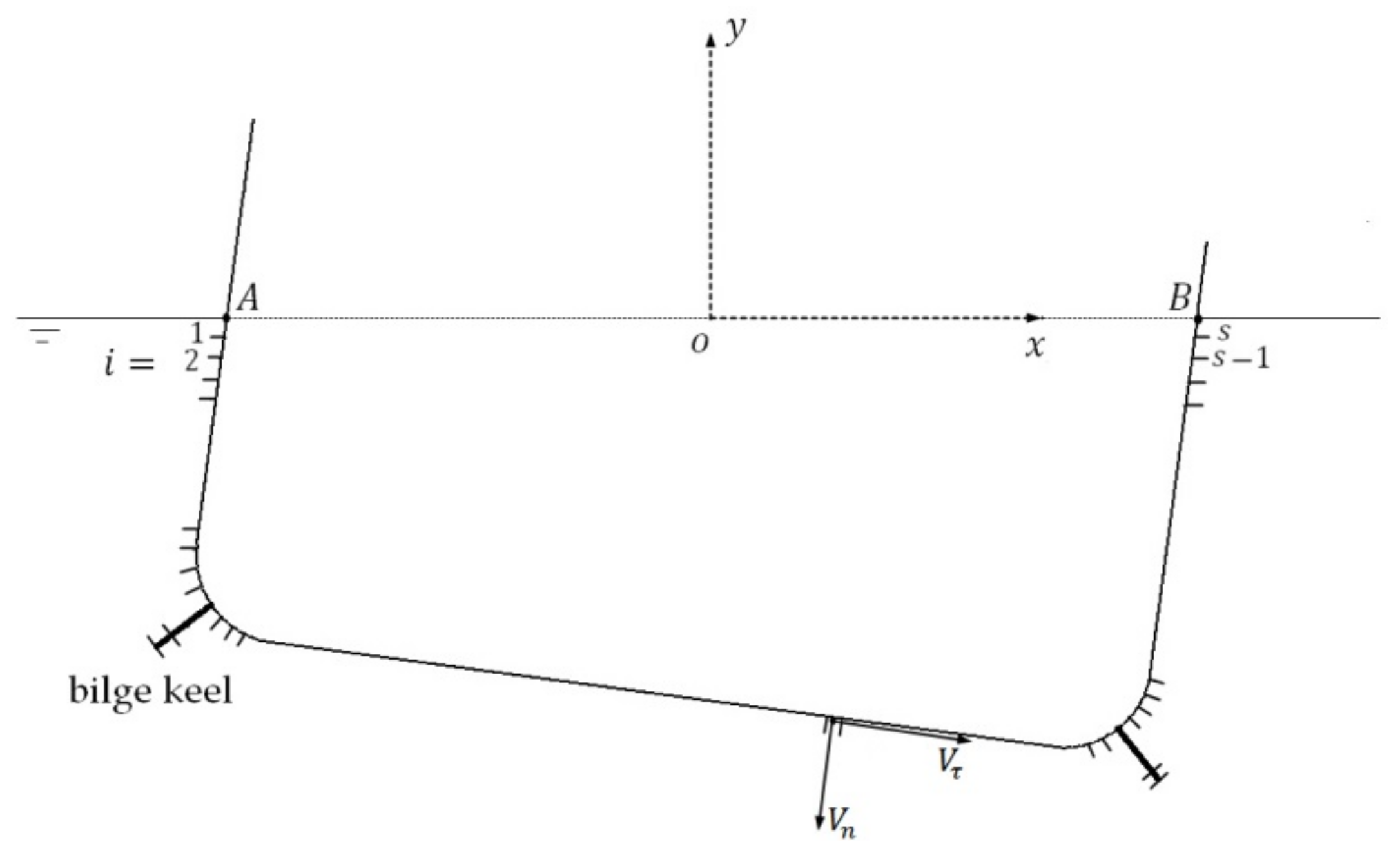
A right-hand Cartesian coordinate system $o-xy$ is defined with $ox$ axis placed on the undisturbed water surface and the $oy$ axis orienting positively upward. Figure 1 portrays the coordinate system $o-xy$ and a hull section with bilge keels.

The differential equation of roll with equivalent linear damping can be written as

$$\left(a_{44}+I_{44}\right)\ddot{\theta }+b_{44}\dot{\theta }+C\left(\theta \right)=F_{44}\left(t\right)$$

(1)

where $a_{44}$ is the added mass, $b_{44}$ is the equivalent linear damping coefficient, $C\left(\theta \right)$ is the stiffness, and $F_{44}\left(t\right)$ is the external roll moment. In this paper, the attention is mainly focused on the evaluation of the equivalent linear damping coefficient $b_{44}$.

2.1. Definite Problem of the $TGF\_N\_V$

Let $\psi \left(x,y,t\right)$ be the disturbed velocity potential of water due to the roll motion of a floating body. Let $\Omega$, $S_{\mathrm{F}}$, $S_{\mathrm{B}}\left(t\right)$, $S_{\infty }$ be the water domain, undisturbed water surface, instantaneous wetted surface of the floating body, and flow boundary at infinity, respectively. The definite conditions for the disturbed velocity potential $\psi \left(x,y,t\right)$ can be formulated as

$$\{\begin{array}{ll}\begin{array}{c}\frac{{\partial }^2\psi }{\partial x^2}+\frac{{\partial }^2\psi }{\partial y^2}=0,\end{array}\hfill & \mathrm{in}\Omega \hfill \\ \frac{{\partial }^2\psi }{\partial t^2}+\mathrm{g}\frac{\partial \psi }{\partial y}+2ϵ{\omega }_0\frac{\partial \psi }{\partial t}=0,\hfill & \mathrm{on}{S}_{\mathrm{F}}\hfill \\ \frac{\partial \psi }{\partial n}=V_n\left(t\right),\hfill & \mathrm{on}{S}_{\mathrm{B}}\left(t\right)\hfill \\ \psi =0,\nabla \psi =0,\hfill & \mathrm{on}{S}_{\infty }\hfill \\ \psi =0,\frac{\partial \psi }{\partial t}=0,\hfill & \mathrm{when}t=0\hfill \end{array}$$

(2)

where $ϵ$ is the non-dimensional viscosity coefficient, ${\omega }_0$ is the reference frequency, and $V_n\left(t\right)$ is the normal velocity of the instantaneous wetted surface.

From Equation (2), one can observe that in the definite conditions of the $\mathrm{TGF}\_\mathrm{N}\_\mathrm{V}$, the normal velocity $V_n\left(t\right)$ is satisfied on the instantaneous wetted surface of the floating body, while the normal velocity in $\mathrm{TGF}\_\mathrm{V}$ [21] is given on the mean wetted surface $S_{\mathrm{B}}\left(t\right)$ of the floating body. This difference makes the definite problem of the $\mathrm{TGF}\_\mathrm{N}\_\mathrm{V}$ to be body-nonlinear.

2.2. Green’s Function for the $TGF\_N\_V$

Analogous to the $\mathrm{TGF}\_\mathrm{V}$ [21], the Green’s function method is employed to solve the Equation (2). Let $G\left(\mathit{p},t;\mathit{q},\tau ;ϵ\right)$ be the Green’s function, which can be expressed as the combination of instantaneous term $\overline{G}\left(\mathit{p},\mathit{q};ϵ\right)$ and free-surface memory term $\tilde{G}\left(\mathit{p},t;\mathit{q},\tau ;ϵ\right)$.

$$G\left(\mathit{p},t;\mathit{q},\tau ;ϵ\right)=\delta \left(t-\tau \right)\overline{G}\left(\mathit{p},\mathit{q};ϵ\right)-H\left(t-\tau \right)\tilde{G}\left(\mathit{p},t;\mathit{q},\tau ;ϵ\right)$$

(3)

where $\delta (·)$ is the Dirac function, $H(·)$ is the Heaviside function, $\mathit{p}\left(x,y\right)$ is the field point, $\mathit{q}\left(\xi ,\eta \right)$ is the source point, $\xi ,\eta$ is the coordinate of $\mathit{q}$ at $ox$ and $oy$ axis, respectively, $\tau$ is the time when $\mathit{q}$ pulses, and $ϵ$ is the non-dimensional viscosity coefficient.

According to the definition of Green’s function, the free-surface memory term should satisfy the following definite conditions:

$$\{\begin{array}{ll}\begin{array}{c}{\nabla }_q^2\tilde{G}=0,\end{array}\hfill & \mathit{p},\mathit{q}\in \Omega ,t>\tau \hfill \\ \frac{{\partial }^2\tilde{G}}{\partial {\tau }^2}+\mathrm{g}\frac{\partial \tilde{G}}{\partial \eta }-2ϵ{\omega }_0\frac{\partial \tilde{G}}{\partial \tau }=0,\hfill & \begin{array}{c}\eta =0\end{array}\hfill \\ {\nabla }_q\tilde{G}=0,\hfill & \mathit{q}\in S_{\infty }\hfill \\ \tilde{G}=0,\hfill & t=\tau \hfill \end{array}$$

(4)

where the subscript $\mathit{q}$ from ${\nabla }_q,{\nabla }_q^2$ means that the operation is taken with respect to variable $\mathit{q}\left(\xi ,\eta \right)$. In the second equation of (4), the sign of the viscous term changes to minus due to the relation $\partial \tilde{G}/\partial \tau =-\partial \tilde{G}/\partial t$.

Obviously, the definite conditions given in Equation (4) are the same as those in Guo et al. [21], i.e., they are not related to the body condition. Thereby, according to Guo et al. [21], the expression of the free-surface memory term $\tilde{G}\left(\mathit{p},t;\mathit{q},\tau ;ϵ\right)$ is

$$\tilde{G}=2{{\displaystyle \int }}_0^{\infty }\sqrt{\frac{\mathrm{g}}{k}}{\mathrm{e}}^{\left(k+{ϵ}^2{k}_0\right)\left(y+\eta \right)}{\mathrm{e}}^{-ϵ{\omega }_0\left(t-\tau \right)}\cos \left(\left(k+{ϵ}^2{k}_0\right)\left(x-\xi \right)\right)\sin \left(\sqrt{\mathrm{g}k}\left(t-\tau \right)\right)\mathrm{d}k$$

(5)

where $k_0={\omega }_0^2/\mathrm{g}$ is the reference wave number in deep water conditions.

On the other hand, the definite conditions for the instantaneous term $\overline{G}$ are associated with the free-surface memory term $\tilde{G}$. The derivation of definite conditions for $\overline{G}$ is detailed in Appendix A, and the final results are shown in Equation (A8), which are the same as those in Guo et al. [21]. According to Appendix B of Guo et al. [21], the unknown constant is $\beta =1$. Therefore, the final definite conditions for $\overline{G}$ are as follows:

$$\{\begin{array}{ll}\begin{array}{l}\begin{array}{c}{\nabla }_q^2\overline{G}=\delta \left(\mathit{p}-\mathit{q}\right),\end{array}\hfill \end{array}\hfill & \begin{array}{l}\mathit{p},\mathit{q}\in \Omega ,t>\tau \hfill \end{array}\hfill \\ \overline{G}=0,\hfill & \eta =0\hfill \\ \overline{G}~O\left(\frac{1}{r_{pq}}\right),\hfill & r_{pq}\to \infty \hfill \\ \frac{\partial \overline{G}}{\partial \eta }=-\frac{1}{\mathrm{g}}\frac{\partial \tilde{G}}{\partial \tau },\hfill & t=\tau ,\eta =0\hfill \end{array}.$$

(6)

where $r_{pq}$ is the distance between field point $\mathit{p}$ and source point $\mathit{q}$.

Since the definite conditions for the instantaneous term $\overline{G}$ and the expression of free-surface memory term $\tilde{G}$ are the same as those in Guo et al. [21], the expression of the instantaneous term $\overline{G}$ must also be the same as that in Guo et al. [21], i.e.,

$$\overline{G}\left(\mathit{p},\mathit{q};ϵ\right)=\mathrm{Re}\left\{E_1\left(-{ϵ}^2{k}_0{R}_{p\overline{q}}\right)-E_1\left(-{ϵ}^2{k}_0{R}_{pq}\right)\right\}$$

(7)

where

$$\{\begin{array}{l}{R}_{p\overline{q}}=y+\eta +\mathrm{i}\left(x-\xi \right)\hfill \\ R_{pq}=-\left|y-\eta \right|+\mathrm{i}\left(x-\xi \right)\hfill \end{array}$$

(8)

$E_1\left(z\right)$ is the complex exponential integral function defined as

$$E_1\left(z\right)={{\displaystyle \int }}_z^{\infty }\frac{{\mathrm{e}}^{-r}}{r}\mathrm{d}r,z\ne 0$$

(9)

2.3. Boundary Integral Equation for the $TGF\_N\_V$

According to (A7) in Appendix A, one can obtain the boundary integral equation

$$\begin{array}{c}2\mathsf{\pi }\psi \left(t,\mathit{p}\right)+{{\displaystyle \int }}_{S_{\mathrm{B}}\left(t\right)}\left(\overline{G}\frac{\partial \psi \left(t,\mathit{q}\right)}{\partial n_q}-\psi \left(t,\mathit{q}\right)\frac{\partial \overline{G}}{\partial n_q}\right)\mathrm{d}{s}_q={{\displaystyle \int }}_0^t\mathrm{d}\tau {{\displaystyle \int }}_{S_{\mathrm{B}}\left(t\right)}\left(\tilde{G}\frac{\partial \psi \left(\tau ,\mathit{q}\right)}{\partial n_q}-\psi \left(\tau ,\mathit{q}\right)\frac{\partial \tilde{G}}{\partial n_q}\right)\mathrm{d}{s}_q\\ +\frac{1}{\mathrm{g}}{{\displaystyle \int }}_0^t\left(\psi \left(\tau ,\mathit{q}\right)\frac{\partial \tilde{G}}{\partial \tau }-\tilde{G}\frac{\partial \psi \left(\tau ,\mathit{q}\right)}{\partial \tau }-2ϵ{\omega }_0\psi \left(\tau ,\mathit{q}\right)\tilde{G}\right)\dot{\xi }\left(\tau \right)|\begin{array}{l}B\hfill \\ A\hfill \end{array}\mathrm{d}\tau \end{array}$$

(10)

where $A$ and $B$ are water surface—wetted surface of the hull intersections (see Figure 1).

The boundary integral Equation (10) is different from that in Guo et al. [21]. There is an addition term at the right end of Equation (10) that reveals the body-nonlinear effect, while there is no similar term in boundary integral equation from Guo et al. [21].

The boundary integral Equation (10) is a mixed source and dipole distribution model. One might prefer the pure source distribution model in numerical practice. Let ${\psi }_{\mathrm{i}}$ be the velocity potential of the flow in the interior of the floating body. Through the same procedure, one can obtain the boundary integral equation with respect to ${\psi }_{\mathrm{i}}$ as follows:

$$\begin{array}{c}{{\displaystyle \int }}_{S_{\mathrm{B}}\left(t\right)}\left(\overline{G}\frac{\partial {\psi }_{\mathrm{i}}\left(t,\mathit{q}\right)}{\partial n_q}-{\psi }_{\mathrm{i}}\left(t,\mathit{q}\right)\frac{\partial \overline{G}}{\partial n_q}\right)\mathrm{d}{s}_q={{\displaystyle \int }}_0^t\mathrm{d}\tau {{\displaystyle \int }}_{S_{\mathrm{B}}\left(t\right)}\left(\tilde{G}\frac{\partial {\psi }_{\mathrm{i}}\left(\tau ,\mathit{q}\right)}{\partial n_q}-{\psi }_{\mathrm{i}}\left(\tau ,\mathit{q}\right)\frac{\partial \tilde{G}}{\partial n_q}\right)\mathrm{d}{s}_q\\ +\frac{1}{\mathrm{g}}{{\displaystyle \int }}_0^t\left({\psi }_{\mathrm{i}}\left(\tau ,\mathit{q}\right)\frac{\partial \tilde{G}}{\partial \tau }-\tilde{G}\frac{\partial {\psi }_{\mathrm{i}}\left(\tau ,\mathit{q}\right)}{\partial \tau }-2ϵ{\omega }_0{\psi }_{\mathrm{i}}\left(\tau ,\mathit{q}\right)\tilde{G}\right)\dot{\xi }\left(\tau \right)|\begin{array}{l}B\hfill \\ A\hfill \end{array}\mathrm{d}\tau \end{array}$$

(11)

It is assumed that the following conditions are satisfied on the wetted surface of the hull:

$$\{\begin{array}{cc}\begin{array}{l}\psi \left(\tau ,\mathit{q}\right)={\psi }_{\mathrm{i}}\left(\tau ,\mathit{q}\right)\hfill \\ \sigma \left(\tau ,\mathit{q}\right)=\frac{\partial \psi \left(\tau ,\mathit{q}\right)}{\partial n_q}-\frac{\partial {\psi }_{\mathrm{i}}\left(\tau ,\mathit{q}\right)}{\partial n_q}\hfill \end{array},& \mathrm{on}{S}_{\mathrm{B}}\left(t\right)\end{array}$$

(12)

where $\sigma$ is the source density.

Subtracting Equation (11) from Equation (10) and taking Equation (12) into consideration yields

$$\begin{array}{l}2\mathsf{\pi }\psi \left(t,\mathit{p}\right)+{{\displaystyle \int }}_{S_{\mathrm{B}}\left(t\right)}\sigma \left(t,\mathit{q}\right)\overline{G}\mathrm{d}{s}_q\\ ={{\displaystyle \int }}_0^t\mathrm{d}\tau {{\displaystyle \int }}_{S_{\mathrm{B}}\left(t\right)}\sigma \left(\tau ,\mathit{q}\right)\tilde{G}\mathrm{d}{s}_q-\frac{1}{\mathrm{g}}{{\displaystyle \int }}_0^t\left(\frac{\partial \psi \left(\tau ,\mathit{q}\right)}{\partial \tau }-\frac{\partial {\psi }_{\mathrm{i}}\left(\tau ,\mathit{q}\right)}{\partial \tau }\right)\tilde{G}\dot{\xi }\left(\tau \right)|\begin{array}{l}B\hfill \\ A\hfill \end{array}\mathrm{d}\tau \end{array}$$

(13)

According to Duan [25],

$$\frac{\partial \psi \left(\tau ,\mathit{q}\right)}{\partial \tau }-\frac{\partial {\psi }_{\mathrm{i}}\left(\tau ,\mathit{q}\right)}{\partial \tau }=-\sigma \left(\tau ,\mathit{q}\right)n_x\dot{\xi }\left(\tau \right)$$

(14)

where $n_x$ is the horizontal component of the normal vector on the intersection of the wetted surface.

Substituting Equations (14) into (13), one gets a boundary integral equation only with source points distributing on the instantaneous wetted body surface.

$$2\mathsf{\pi }\psi \left(t,\mathit{p}\right)+{{\displaystyle \int }}_{S_{\mathrm{B}}\left(t\right)}\sigma \left(t,\mathit{q}\right)\overline{G}\mathrm{d}{s}_q={{\displaystyle \int }}_0^t\mathrm{d}\tau {{\displaystyle \int }}_{S_{\mathrm{B}}\left(t\right)}\sigma \left(\tau ,\mathit{q}\right)\tilde{G}\mathrm{d}{s}_q+\frac{1}{\mathrm{g}}{{\displaystyle \int }}_0^t\sigma \left(\tau ,\mathit{q}\right)n_x\tilde{G}\dot{\xi }{\left(\tau \right)}^2|\begin{array}{l}B\hfill \\ A\hfill \end{array}\mathrm{d}\tau$$

(15)

Taking the derivative of (15) with respect to normal vector ${\mathit{n}}_p$ on point $\mathit{p}$, the source density boundary integral equation is obtained.

$$\begin{array}{l}-\mathsf{\pi }\sigma \left(t,\mathit{p}\right)+{{\displaystyle \int }}_{S_{\mathrm{B}}\left(t\right)}\sigma \left(t,\mathit{q}\right)\frac{\partial \overline{G}}{\partial n_p}\mathrm{d}{s}_q\\ =-2\mathsf{\pi }{V}_n\left(t,\mathit{p}\right)+{{\displaystyle \int }}_0^t\mathrm{d}\tau {{\displaystyle \int }}_{S_{\mathrm{B}}\left(t\right)}\sigma \left(\tau ,\mathit{q}\right)\frac{\partial \tilde{G}}{\partial n_p}\mathrm{d}{s}_q+\frac{1}{\mathrm{g}}{{\displaystyle \int }}_0^t\sigma \left(\tau ,\mathit{q}\right)n_x\frac{\partial \tilde{G}}{\partial n_p}\dot{\xi }{\left(\tau \right)}^2|\begin{array}{l}B\hfill \\ A\hfill \end{array}\mathrm{d}\tau \end{array}$$

(16)

where $V_n\left(t,\mathit{p}\right)$ is the velocity of point $\mathit{p}$ in the outward normal direction.

2.4. Equivalent Roll Damping Using the $TGF\_N\_V$

The Bernoulli’s equation with consideration of viscous dissipation effects of water can be written as

$$\frac{\partial \psi }{\partial t}+\frac{P}{\mathsf{\rho }}+\mathrm{g}\eta +\frac{1}{2}{\left(\nabla \psi \right)}^2+2ϵ{\omega }_0\psi =0$$

(17)

where $P$ is the overall pressure, which can be decomposed into the sum of hydrostatic pressure $p_0$ and hydrodynamic pressure $p$

$$P=p_0+p$$

(18)

$$\frac{p_0}{\mathsf{\rho }}+\mathrm{g}\eta =0$$

(19)

The hydrostatic pressure $p_0$ relates only to the immersion depth of the wetted surface, while the roll damping associates only with roll angular velocity, according to Equation (1). Therefore $p_0$ does not make contribution to the roll damping.

Subtracting Equation (19) from Equation (17) yields

$$\frac{\partial \psi }{\partial t}+\frac{p}{\mathsf{\rho }}+\frac{1}{2}{\left(\nabla \psi \right)}^2+2ϵ{\omega }_0\psi =0$$

(20)

Then the roll moment of the floating body due to hydrodynamic pressure is

$$f\left(t\right)=-\mathsf{\rho }{{\displaystyle \int }}_{S_{\mathrm{B}}\left(t\right)}\frac{\partial \psi }{\partial t}{n}_{\mathrm{c}}\mathrm{d}s-\mathsf{\rho }{{\displaystyle \int }}_{S_{\mathrm{B}}\left(t\right)}\left(\frac{1}{2}{\left(\nabla \psi \right)}^2+2ϵ{\omega }_0\psi \right)n_{\mathrm{c}}\mathrm{d}s$$

(21)

where $n_{\mathrm{c}}$ is the generalized normal vector on the wetted surface defined as

$$n_{\mathrm{c}}=\stackrel{\rightharpoonup }{r}\times \stackrel{\rightharpoonup }{n}=\left(x,y\right)\times \left(n_x,n_y\right)=x{n}_y-y{n}_x$$

(22)

To enhance the numerical stability, the first term on the right-hand side of Equation (21) can be transformed using Reynold’s transport theorem [25]

$${{\displaystyle \int }}_{S_{\mathrm{B}}\left(t\right)}\frac{\partial \psi }{\partial t}{n}_{\mathrm{c}}\mathrm{d}s=\frac{\mathrm{d}}{\mathrm{d}t}{{\displaystyle \int }}_{S_{\mathrm{B}}\left(t\right)}\psi n_{\mathrm{c}}\mathrm{d}s-{{\displaystyle \int }}_{S_{\mathrm{B}}\left(t\right)}\left(\stackrel{\rightharpoonup }{r}\times \nabla \psi \right)V_n\mathrm{d}s-\psi \dot{x}\left(t\right)(\stackrel{\rightharpoonup }{r}\times \stackrel{\rightharpoonup }{j})|\begin{array}{l}B\hfill \\ A\hfill \end{array}$$

(23)

The calculation of $\stackrel{\rightharpoonup }{r}\times \nabla \psi$ and ${\left|\nabla \psi \right|}^2$ was not detailed in Duan [25]. In this paper we would like to provide a possible approach to calculate them. As shown in Figure 1, $V_{\tau }$ is the tangential velocity of water on the wetted surface, which can be obtained through the numerical difference

$$V_{\tau }^i=\frac{{\psi }_{i+1}-{\psi }_{i-1}}{2∆s}$$

(24)

where $∆s$ is the segment length, $i$ is the segment index for the wetted surface.

Now, one can obtain the following expressions:

$${\left(\nabla \psi \right)}^2=V_n{}^2+V_{\tau }{}^2$$

(25)

$$\begin{array}{l}\stackrel{\rightharpoonup }{r}\times \nabla \psi =\left(x,y\right)\times \left({\psi }_x,{\psi }_y\right)=\left(x,y\right)\times \left(n_x{V}_n+n_y{V}_{\tau },n_y{V}_n-n_x{V}_{\tau }\right)\\ =V_n\left(x{n}_y-y{n}_x\right)-V_{\tau }\left(x{n}_x+y{n}_y\right)=V_n{n}_{\mathrm{c}}-V_{\tau }{n}_{\mathrm{d}}\end{array}$$

(26)

where $n_{\mathrm{d}}$ is the dot product of $\stackrel{\rightharpoonup }{r}$ and $\stackrel{\rightharpoonup }{n}$.

Substituting Equations (23) into (21), and then substituting Equations (25) and (26) into the resulting equation, one gets roll moment

$$\begin{array}{c}f\left(t\right)=-\rho \frac{\mathrm{d}}{\mathrm{d}t}{{\displaystyle \int }}_{S_{\mathrm{B}}\left(t\right)}\psi n_{\mathrm{c}}\mathrm{d}s-\rho {{\displaystyle \int }}_{S_{\mathrm{B}}\left(t\right)}\left(\frac{1}{2}\left(V_{\tau }{}^2-V_n{}^2\right)+2ϵ{\omega }_0\psi \right)n_{\mathrm{c}}\mathrm{d}s-\rho {{\displaystyle \int }}_{S_{\mathrm{B}}\left(t\right)}{V}_n{V}_{\tau }{n}_{\mathrm{d}}\mathrm{d}s\hfill \\ +\rho \psi \dot{x}\left(t\right)x|\begin{array}{l}B\hfill \\ A\hfill \end{array}\hfill \end{array}$$

(27)

Once the time series of the roll moment is obtained, the equivalent roll damping can be calculated using the cosine Fourier transform [16]

$$b_{44}=\frac{1}{\mathsf{\pi }}{{\displaystyle \int }}_{nT}^{\left(n+1\right)T}\mathrm{Im}\left\{f\left(t\right)\right\}\cos \omega t\mathrm{d}t$$

(28)

where $T$ is the period of roll, $\mathrm{Im}\{·\}$ takes the imaginary part of the complex number. The integral in Equation (28) starts from the time $nT$, when the time series has reached a steady state. The imaginary part of $f\left(t\right)$ is selected for calculation due to that the imaginary part of roll ($\mathrm{Im}\{\dot{\theta }\}$) reaches to its maximum angular velocity at time $nT$ and $\left(n+1\right)T$.

Generally, the quantities related to roll damping need to be made dimensionless for the convenience of use or comparison. In this paper the roll frequency, roll damping, and roll moment are nondimensionalized as follows:

$$\tilde{\omega }=\frac{\omega }{\sqrt{\mathrm{g}/d}}$$

(29)

$${\tilde{b}}_{44}=\frac{b_{44}}{4\rho b{d}^3\sqrt{\mathrm{g}/d}}$$

(30)

where $b,d$ are beam and mean draft of the hull section.

3. Application of the $\mathbf{TGF}\mathbf{\_}\mathbf{N}\mathbf{\_}\mathbf{V}$ for Solving Roll Damping of Hull Sections with Bilge Keels

A novel body-nonlinear Green’s function method with viscous dissipation effects ($\mathrm{TGF}\_\mathrm{N}\_\mathrm{V}$) was developed in Section 2. In this section, $\mathrm{TGF}\_\mathrm{N}\_\mathrm{V}$ is employed to solve the roll damping of hull sections with bilge keels under small and large roll amplitude. For comparison purpose, numerical results from linear inviscid time-domain Green’s function method ($\mathrm{TGF}$) [25], body-nonlinear inviscid time-domain Green’s function method ($\mathrm{TGF}\_\mathrm{N}$) [25], and experimental fluid dynamic (EFD) results [13] are also provided in the cases.

3.1. Hull Section Under Small Amplitude Roll

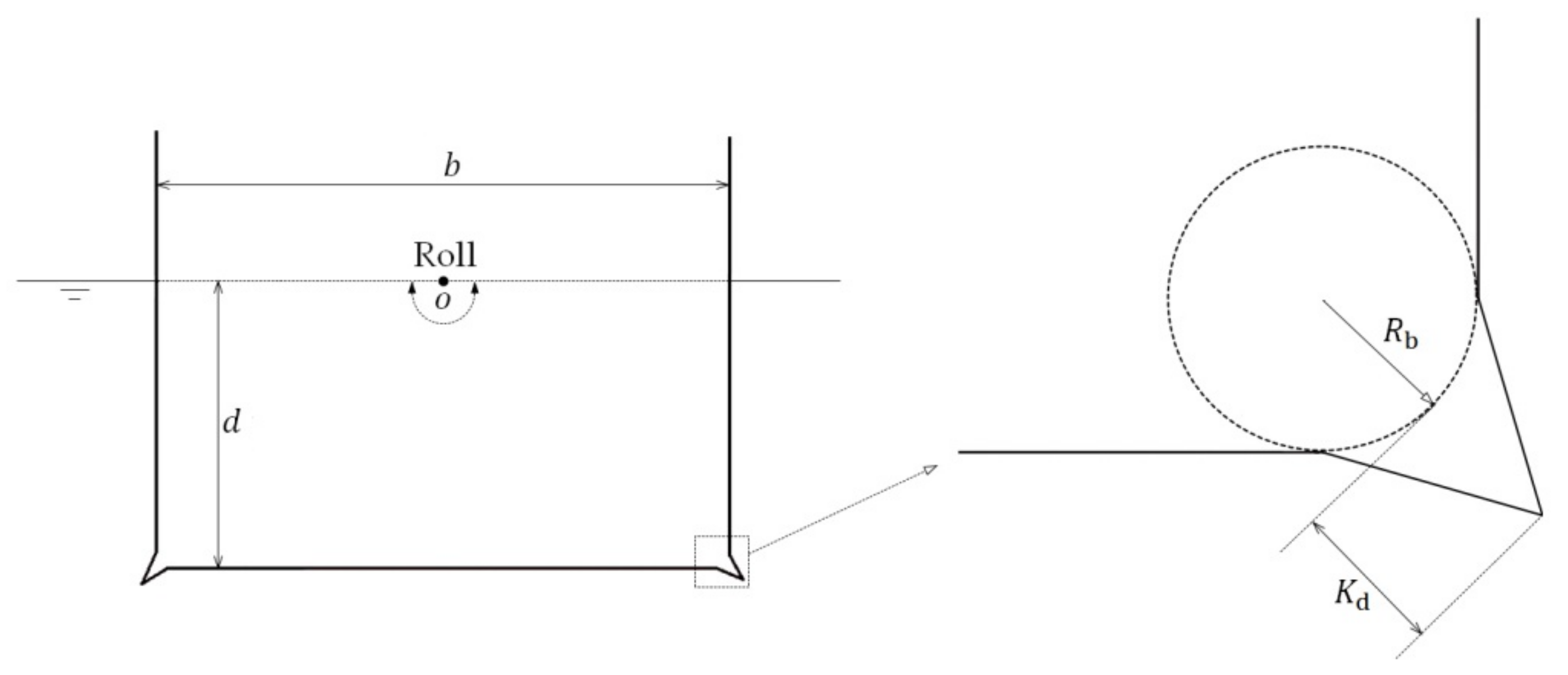
A rectangular hull section with bilge keels is shown in Figure 2. The beam and mean draught of the hull section are $b=0.4\mathrm{m}$ and $d=0.2\mathrm{m}$, respectively. Two bilge keels are set at the corners that connect the wall and bottom of the hull section, and the bilge radius and bilge keel depth are $R_{\mathrm{b}}=0.02b$ and $K_{\mathrm{d}}=0.04b$, respectively. The hull section harmonically rolls on the water surface with small amplitude $\theta =0.05\mathrm{rad}\approx {2.87}^{\circ }$. The axis of rotation is located at the center of waterplane of the hull section. The detailed description of the experiments can be found in Yeung et al. [13].

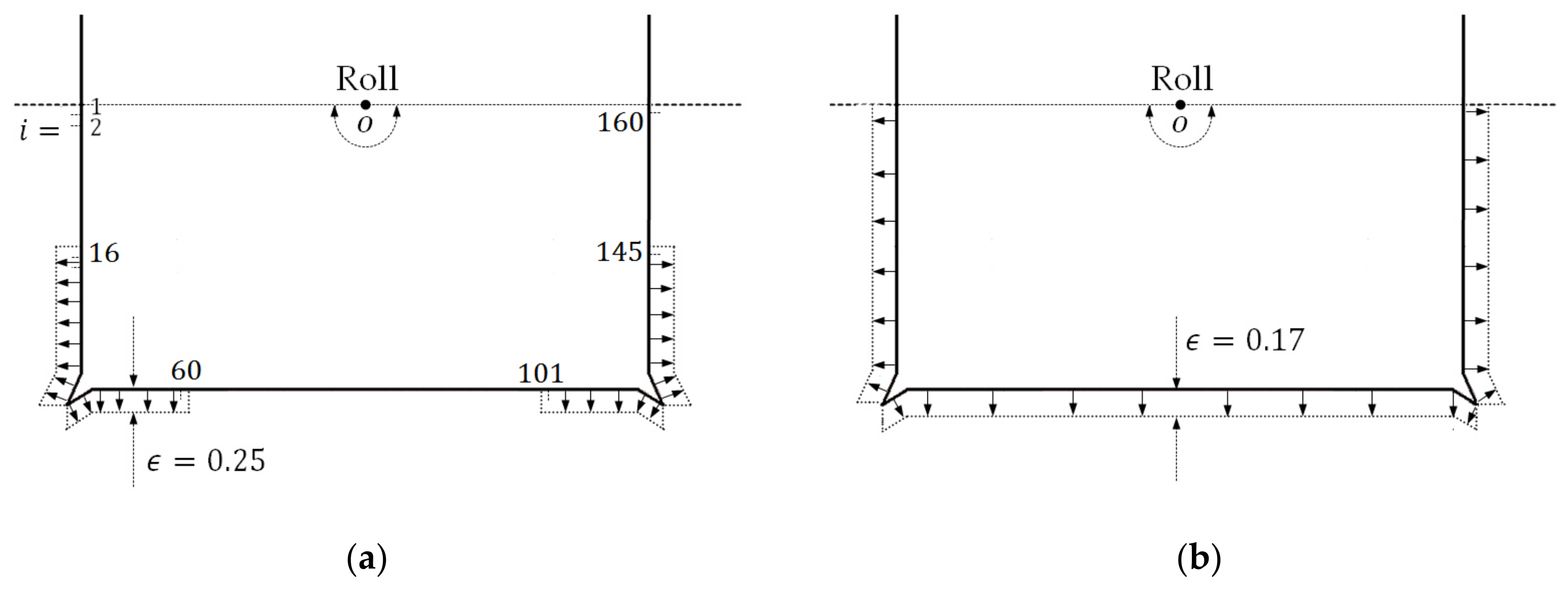
As abovementioned, the novel Green’s function method $\mathrm{TGF}\_\mathrm{N}\_\mathrm{V}$ and two contrast methods ($\mathrm{TGF}$ and $\mathrm{TGF}\_\mathrm{N}$ [25]) are employed for the roll damping calculation. In each Green’s function method, the hull section is discretized into 160 segments (30 for each wall, 20 for each bilge keel, 60 for the flat bottom). In the linear method $\mathrm{TGF}$, all segments are located on the mean wetted surface of the hull section and kept constant. On the other hand, in the nonlinear methods $\mathrm{TGF}\_\mathrm{N}$ and $\mathrm{TGF}\_\mathrm{N}\_\mathrm{V}$, all segments move with roll motion, and the segments on two sidewalls need to be remeshed due to the change of draught.

Two viscosity distribution approaches are adopted for $\mathrm{TGF}\_\mathrm{N}\_\mathrm{V}$ in this case. As shown in Figure 3a, in the first approach a non-zero viscosity is set only on the segments in the vicinity of bilge keels ($16\le i\le 60,101\le i\le 145$), while on the rest segments the viscosity is set to zero. In the second approach (see Figure 3b) a non-zero viscosity is set on all segments ($1\le i\le 160$). The non-dimensional viscosity coefficient $ϵ$ should be empirically selected or obtained through the CFD or EFD methods. It is found that desirable results can be achieved if taking the non-dimensional viscosity coefficient as $ϵ=0.25$ for the first approach and $ϵ=0.17$ for the second approach. The roll frequency $\omega$ is taken as the reference frequency ${\omega }_0$ in $\mathrm{TGF}\_\mathrm{N}\_\mathrm{V}$ (see Equation (27)).

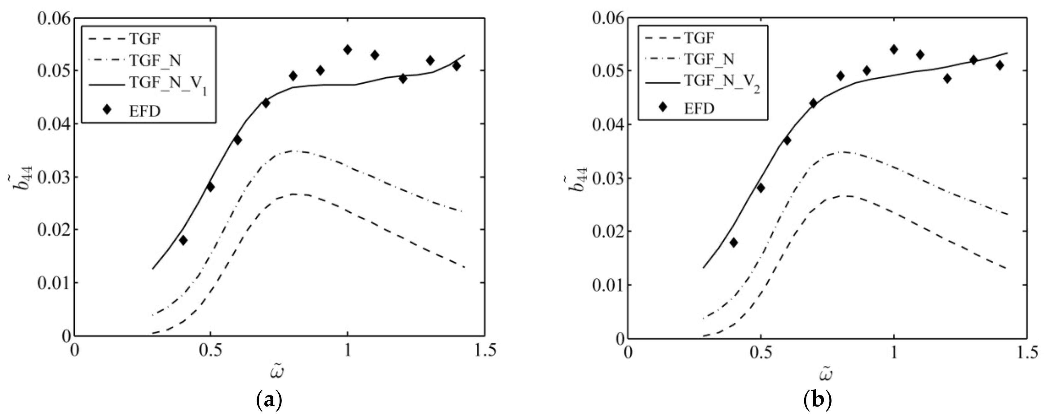
Figure 4 portrays the equivalent roll damping using $\mathrm{TGF}$, $\mathrm{TGF}\_\mathrm{N}$, and $\mathrm{TGF}\_\mathrm{N}\_\mathrm{V}$ as compared with EFD. The lines labeled with “$\mathrm{TGF}\_\mathrm{N}\_{\mathrm{V}}_1$” and “$\mathrm{TGF}\_\mathrm{N}\_{\mathrm{V}}_2$” denote results from $\mathrm{TGF}\_\mathrm{N}\_\mathrm{V}$ by using the first and second viscosity distribution approach, respectively. Comparing the $\mathrm{TGF}\_\mathrm{N}\_{\mathrm{V}}_1$ result with the $\mathrm{TGF}\_\mathrm{N}\_{\mathrm{V}}_2$ one, one can find that both of two viscosity distribution approaches are effective for evaluating the roll damping of a hull section with bilge keels. Nonetheless, it can be observed that the second approach can yield smoother results. Thereby, in the next case, only the second viscosity distribution approach will be employed for study.

From Figure 4, one can observe that, as compared with EFD data, the linear inviscid method $\mathrm{TGF}$ and body-nonlinear inviscid method $\mathrm{TGF}\_\mathrm{N}$ significantly underestimate the roll damping, though the discrepancy between $\mathrm{TGF}\_\mathrm{N}$ result and EFD data is smaller than that between the $\mathrm{TGF}$ result and EFD data, which suggests that the numerical results could be improved when the nonlinear effects are taken into account. Moreover, the $\mathrm{TGF}$ and $\mathrm{TGF}\_\mathrm{N}$ results decrease when $\tilde{\omega }>0.8$, which are in the opposite trend as compared to EFD data. On the other hand, the $\mathrm{TGF}\_\mathrm{N}\_\mathrm{V}$ results agree well with EFD data under the given non-dimensional viscosity coefficients, even when $\tilde{\omega }>0.8$.

The numerical results in this case suggest that, for the hull section with bilge keels under roll motion of small amplitude, the viscous effects in the roll damping are more important than the nonlinear effects. The study also confirms the possibility of employing $\mathrm{TGF}\_\mathrm{N}\_\mathrm{V}$ to estimate the viscous effects as well as nonlinear effects of a hull section with bilge keels rolling on the free surface. In contrast, the inviscid methods $\mathrm{TGF}$ and $\mathrm{TGF}\_\mathrm{N}$ are not appropriate for evaluating the roll damping of the hull section with bilge keels.

3.2. Hull Section Under Large Amplitude Roll

Figure 5 depicts an S60 midship section with bilge keels. The beam and mean draught of the hull section are $b=0.237\mathrm{m}$ and $d=0.057\mathrm{m}$, respectively. The bilge radius and bilge keel depth are $R_{\mathrm{b}}=0.035\mathrm{m}$ and $K_{\mathrm{d}}=0.01\mathrm{m}$, respectively. The single degree of freedom model experiment was carried out by Yıldız et al. [15], in which the S60 midship section model is fixed by a forced rolling device, and the roll moment is measured through the torque transducer. The S60 midship section model harmonically rolls on the water surface with large amplitudes $\theta =0.15\mathrm{rad}\left({8.59}^{\circ }\right),0.20\mathrm{rad}\left({11.6}^{\circ }\right),0.25\mathrm{rad}\left({14.4}^{\circ }\right)$. The axis of rotation is located at the center of waterplane of the hull section. More detailed description on the model experiments can be found in Yıldız et al. [15].

As in the previous case, the S60 midship section is discretized into 160 segments (30 for each wall, 20 for each bilge keel, 60 for the flat bottom). It is worth mention that the bilge keels in this case are simplified to lines without thickness, and each side of the bilge keel is discretized into 10 segments. The numerical error may occur when the source point and field point located on the two sides of the bilge keel are overlapped. To avoid this, the value of the Green’s function is set as zero once the source point and field point are overlapped. Note that for the body-nonlinear methods, the segments on walls could be stretched or compressed with the roll motion of the S60 midship section. The second viscosity distribution approach, i.e., a non-zero viscosity for all segments on the wetted surface, is employed for $\mathrm{TGF}\_\mathrm{N}\_\mathrm{V}$ in this case. It is found that for $\mathrm{TGF}\_\mathrm{N}\_\mathrm{V}$ the non-dimensional viscosity coefficient $ϵ=0.2,0.25,0.3$ for the roll motion with amplitude $\theta =0.15,0.20,0.25\left(\mathrm{rad}\right),$ respectively, could lead to desirable results. It can be noted that for larger roll amplitudes, it requires larger non-dimensional viscosity coefficient for $\mathrm{TGF}\_\mathrm{N}\_\mathrm{V}$. The roll frequency $\omega$ is taken as the reference frequency ${\omega }_0$ in $\mathrm{TGF}\_\mathrm{N}\_\mathrm{V}$.

Figure 6 portrays the equivalent roll damping using $\mathrm{TGF}$, $\mathrm{TGF}\_\mathrm{N}$ and $\mathrm{TGF}\_\mathrm{N}\_\mathrm{V}$ as compared with CFD [15] and EFD [15]. One can find that, under all roll amplitudes, the linear inviscid method $\mathrm{TGF}$ and body-nonlinear inviscid method $\mathrm{TGF}\_\mathrm{N}$ dramatically underestimate the roll damping as compared with EFD data. Nonetheless, as compared to $\mathrm{TGF}$, the $\mathrm{TGF}\_\mathrm{N}$ results are closer to EFD, which suggests that there exist nonlinear effects in the roll damping. On the other hand, the $\mathrm{TGF}\_\mathrm{N}\_\mathrm{V}$ results agree well with EFD data, though at high roll frequency $\mathrm{TGF}\_\mathrm{N}\_\mathrm{V}$ slightly underestimates the equivalent roll damping. In contrast, the CFD results also agree well with EFD data, though it overestimates the damping at high roll frequency.

The numerical results in this case suggest that for the hull section with bilge keels under large amplitude roll, the viscous effects in the roll damping are much more important than the nonlinear effects, and one could obtain desirable numerical results only when both of nonlinear and viscous effects are considered. The study also confirms the effectiveness of $\mathrm{TGF}\_\mathrm{N}\_\mathrm{V}$ in evaluating the equivalent roll damping of a hull section with bilge keels rolling on the free surface with large amplitude.

4. Conclusions

This paper presents a novel body-nonlinear time-domain Green’s function method ($\mathrm{TGF}\_\mathrm{N}\_\mathrm{V}$) for evaluating the equivalent roll damping of floating bodies on the free surface with viscous dissipation effects. The $\mathrm{TGF}\_\mathrm{N}\_\mathrm{V}$ is derived through the definite problems based on “fairly perfect fluid.” The $\mathrm{TGF}\_\mathrm{N}\_\mathrm{V}$ is different from the existing body-nonlinear time-domain Green’s function ($\mathrm{TGF}\_\mathrm{N}$) [25] or linear time-domain Green’s function method with viscous dissipation effects ($\mathrm{TGF}\_\mathrm{V}$) [21] as follows. As compared to $\mathrm{TGF}\_\mathrm{N}$, the viscous effects of the fluid can be approximately taken into account. As compared to $\mathrm{TGF}\_\mathrm{V}$, the nonlinear effects of the large amplitude roll can be precisely considered.

The $\mathrm{TGF}\_\mathrm{N}\_\mathrm{V}$ is employed to evaluate the equivalent roll damping of hull sections with bilge keels, in which there exist both of viscous and nonlinear effects. The numerical results suggest that the viscous effects are more important than the nonlinear effects in the roll motion, and $\mathrm{TGF}\_\mathrm{N}\_\mathrm{V}$ can give desirable numerical results as compared with CFD or EFD results. In contrast, those inviscid Green’s function methods ($\mathrm{TGF}$ or $\mathrm{TGF}\_\mathrm{N}$) are not appropriate for estimating the equivalent roll damping of hull sections with bilge keels.

References

- Westcott, S.; Abell, R.W.L.G. The Papers of William Froude, 1st ed.; Institution of Naval Architects: London, UK, 1955; pp. 1–74. ISBN B00HHWDU6A. [Google Scholar]
- Nayfeh, A.H.; Mook, D.T. Nonlinear Oscillations, 1st ed.; Wiley: New York, NY, USA, 1979; pp. 39–258. ISBN 0-471-12142-8. [Google Scholar]
- Cardo, A.; Trincas, G. A multiscale analysis of nonlinear rolling. Ocean Eng. 1987, 14, 83–88. [Google Scholar] [CrossRef]
- Taylan, M. Solution of the nonlinear roll model by a generalized asymptotic method. Ocean Eng. 1999, 26, 1169–1181. [Google Scholar] [CrossRef]
- Roberts, J.B. Estimation of nonlinear ship roll damping from free-decay data. J. Ship Res. 1983, 29, 127–138. [Google Scholar]
- Jang, T.S.; Kwon, S.H.; Lee, J.H. Recovering the functional form of the nonlinear roll damping of ships from a free-roll decay experiment: An inverse formulism. Ocean Eng. 2010, 37, 1337–1344. [Google Scholar] [CrossRef]
- Peyton Jones, J.C.; Çankaya, I. Polyharmonic balance analysis of nonlinear ship roll response. Nonlinear Dyn. 2004, 35, 123–146. [Google Scholar] [CrossRef]
- Eissa, M.; EI-Bassiuny, A.F. Analytical and numerical solutions of a non-linear ship rolling motion. Appl. Math. Comput. 2003, 134, 243–270. [Google Scholar] [CrossRef]
- Bass, D.W.; Haddara, M.R. Nonlinear models of ship roll damping. Int. Shipbuild. Prog. 1988, 35, 5–24. [Google Scholar]
- Hou, X.; Zou, Z. SVR-based identification of nonlinear roll motion equation for FPSOs in regular waves. Ocean Eng. 2015, 109, 531–538. [Google Scholar] [CrossRef]
- Huo, C.; Dong, W. Identification of ship roll parameters from free-roll decay based on extended Kalman filtering. J. Wuhan Univ. Technol. 2016, 40, 214–218. (In Chinese) [Google Scholar]
- Sathyaseelan, D.; Hariharan, G.; Kannan, K. Parameter identification for nonlinear damping coefficient from large-amplitude ship roll motion using wavelets. Beni-Suef Univ. J. Basic Appl. Sci. 2017, 6, 138–144. [Google Scholar] [CrossRef]
- Yeung, R.W.; Roddier, D.; Alessandrini, B.; Gentaz, L.; Liao, S. On roll hydrodynamics of cylinders fitted with bilge keels. In Proceedings of the 23rd Symposium on Naval Hydrodynamics, Val de Reuil, France, 17–22 September 2000. [Google Scholar]
- Korpus, R.; Falzarano, J. Prediction of viscous ship roll damping by unsteady navier-stokes techniques. J. Offshore Mech. Arct. 1997, 119, 108–113. [Google Scholar] [CrossRef]
- Yıldız, B.; Çakıcı, F.; Katayama, T.; Yılmaz, H. URANS prediction of roll damping for a ship hull section at shallow draft. J. Mar. Sci. Technol. 2016, 21, 48–56. [Google Scholar] [CrossRef]
- Lavrov, A.; Rodrigues, J.M.; Gadelho, J.; Guedes Soares, C. Calculation of hydrodynamic coefficients of ship sections in roll motion using Navier-Stokes equations. Ocean Eng. 2017, 133, 36–46. [Google Scholar] [CrossRef]
- Liu, X.; Lin, P.; Shao, S. An ISPH simulation of coupled structure interaction with free surface flows. J. Fluids Struct. 2014, 48, 46–61. [Google Scholar] [CrossRef]
- Ikeda, Y.; Himeno, Y.; Tanaka, N. Components of roll damping of ship at forward speed. J. Soc. Naval Arch. Jpn. 2009, 143, 113–125. [Google Scholar] [CrossRef]
- Brown, D.; Patel, M. A theory for vortex shedding from the keels of marine vehicles. J. Eng. Math. 1985, 19, 265–295. [Google Scholar] [CrossRef]
- Downie, M.J.; Dearman, P.W.; Graham, J.M.R. Effect of vortex shedding on the coupled roll response of bodies in waves. J. Fluid Mech. 1988, 189, 243–261. [Google Scholar] [CrossRef]
- Guo, Z.Q.; Ma, Q.W.; Qin, H.D. A time-domain Green’s function for interaction between water waves and floating bodies with viscous dissipation effects. Water 2018, 10, 72. [Google Scholar] [CrossRef]
- Chen, X.B. Hydrodynamics in offshore and naval applications-Part. In Proceedings of the 6th International Conference on Hydrodynamics, Perth, Australia, 24–26 November 2004. [Google Scholar]
- Chen, X.B.; Dias, F. Visco-potential flow and time-harmonic ship waves. In Proceedings of the 25th International Workshop on Water Waves and Floating Bodies (IWWWFB), Harbin, China, 9–12 May 2010. [Google Scholar]
- Wu, G. The Time-Domain Green Function Method Involving Fluid Viscosity. Master’s Thesis, Harbin Engineering University, Harbin, China, 2007. [Google Scholar]
- Duan, W.Y. Nonlinear Hydrodynamic Forces Acting on a Ship Undergoing Large Amplitude Motions. Ph.D. Thesis, Harbin Engineering University, Harbin, China, 1995. [Google Scholar]
- Kacham, B. Inviscid and Viscous 2D Unsteady Flow Solvers Applied to FPSO Hull Roll Motions. Master’s Thesis, The University of Texas at Austin, Austin, TX, USA, 2004. [Google Scholar]
Figure 1.
The coordinate system and a hull section with bilge keels. The hull section harmonically rolls on the water surface. and are water surface—hull wetted surface intersections. The wetted surface of the hull section is discretized into segments.
Figure 2.
A rectangular hull section with bilge keels harmonically rolls on the water surface, with beam , mean draught , bilge radius , bilge keel depth , and roll amplitude . The rotation axis is located at the center of waterplane.
Figure 3.
Two viscosity distribution approaches for . (a) for segments and , while for the rest segments; (b) for all segments.
Figure 4.
Equivalent roll damping using different methods ( [25], [25], ) as compared with experimental fluid dynamic (EFD) data [13,26]. (a) Equivalent roll damping related to the first viscosity distribution approach; (b) Equivalent roll damping related to the second viscosity distribution approach.
Figure 5.
A semi-submerged S60 midship section with bilge keels harmonically rolls in the presence of a free surface; beam , mean draught , bilge radius , bilge keel depth , roll amplitudes . The rotation axis is located at the center of the waterplane.
© 2018 by the authors. Licensee MDPI, Basel, Switzerland. This article is an open access article distributed under the terms and conditions of the Creative Commons Attribution (CC BY) license (http://creativecommons.org/licenses/by/4.0/).
Share and Cite
MDPI and ACS Style
Guo, Z.; Ma, Q.; Yu, S.; Qin, H. A Body-Nonlinear Green’s Function Method with Viscous Dissipation Effects for Large-Amplitude Roll of Floating Bodies. Appl. Sci. 2018, 8, 517. https://doi.org/10.3390/app8040517
AMA Style
Guo Z, Ma Q, Yu S, Qin H. A Body-Nonlinear Green’s Function Method with Viscous Dissipation Effects for Large-Amplitude Roll of Floating Bodies. Applied Sciences. 2018; 8(4):517. https://doi.org/10.3390/app8040517
Chicago/Turabian StyleGuo, Zhiqun, Qingwei Ma, Shuangrui Yu, and Hongde Qin. 2018. "A Body-Nonlinear Green’s Function Method with Viscous Dissipation Effects for Large-Amplitude Roll of Floating Bodies" Applied Sciences 8, no. 4: 517. https://doi.org/10.3390/app8040517
Note that from the first issue of 2016, this journal uses article numbers instead of page numbers. See further details here.