Fault Diagnosis of a Reconfigurable Crawling–Rolling Robot Based on Support Vector Machines

Abstract

As robots begin to perform jobs autonomously, with minimal or no human intervention, a new challenge arises: robots also need to autonomously detect errors and recover from faults. In this paper, we present a Support Vector Machine (SVM)-based fault diagnosis system for a bio-inspired reconfigurable robot named Scorpio. The diagnosis system needs to detect and classify faults while Scorpio uses its crawling and rolling locomotion modes. Specifically, we classify between faulty and non-faulty conditions by analyzing onboard Inertial Measurement Unit (IMU) sensor data. The data capture nine different locomotion gaits, which include rolling and crawling modes, at three different speeds. Statistical methods are applied to extract features and to reduce the dimensionality of original IMU sensor data features. These statistical features were given as inputs for training and testing. Additionally, the c-Support Vector Classification (c-SVC) and nu-SVC models of SVM, and their fault classification accuracies, were compared. The results show that the proposed SVM approach can be used to autonomously diagnose locomotion gait faults while the reconfigurable robot is in operation.

1. Introduction

In the last few decades, robotic applications have drastically increased, and continue to increase, as we advance towards more sophisticated and fast-paced development environments. Modern robots are highly complex mechatronic systems with hardware and software modules that have a diverging set of features. Due to the highly complex nature of next-generation robotic systems, and the uncertain environments they occupy, modern robots are highly likely to encounter faults during runtime. Even well-designed robotic hardware will encounter a fault in its lifetime. Machine learning techniques have been used for automated fault diagnosis in many industrial applications. In [1], the authors proposed a fault diagnosis method for a spur bevel gear box. The statistical features used in this procedure are determined via wavelet coefficients of the vibration signals. This work uses Artificial Neural Networks (ANN), which provided an accuracy of 97.5%, and Proximal Support Vector Machines (SVM), which provided an accuracy of 97% for classification. In [2], Sheng-Fa Yuan proposed a fault detection technique for turbo-pump motors by using a Multi-class Support Vector Machine for classification and Principal Component Analysis (PCA) for dimensionality reduction. This model exhibits a high level of accuracy, in the range of 95% to 100%, when tested with different kinds of Support Vector Machine methods. In [3], a fault diagnosis technique, which uses multiple components, is implemented for rotational mechanical systems using Support Vector Machine and decision tree methods. This work uses the vibration signals of machinery to extract the statistical features needed for classification. A neural network-based fault diagnosis technique for rotational machine parts is presented in [4]. The two neural networks used in this paper were either non-linear radial basis function-based or time delay-based neural networks. It was tested in the automatic gear system of automobiles using their acoustic data. Another similar machine learning-based approach is proposed in [5] for figuring out the faults in ball bearings. A high-speed rotor supported on a ball bearing is used to collect the vibration-signal data; the features are extracted from this data set. The classification is done using Support Vector Machines and Artificial Neural Networks.

Aside from SVM and ANN, various other techniques have been explored in the context of fault diagnosis in industrial settings. In [6], a Non-linear Unknown Input Observer was used to diagnose a malfunctioning part in an autonomous spacecraft used in the rendezvous phase of the Mars Sample Return (MSR) mission. This approach does not involve machine learning. Instead, it uses observers and position models to detect faults. The approach in [7] uses an analytical redundancy method to diagnose faults in a vehicle roll rate sensor. Among the models found in analytical redundancy, an Eigen structure assignment is utilized in this work because it provides a higher level of robustness than other models. Another strategy mentioned in [8] for fault detection in ball bearings uses the three-phase induction motor. This approach uses PCA and Fisher’s Linear Discriminant Analysis (LDA) for dimensionality reduction. Furthermore, it uses random tree algorithms and a C4.5 decision tree algorithm to classify faulty and non-faulty data. In [9], a genetic algorithm approach is used for detecting faults in analog circuits. The parameters used for this process are obtained from the transfer function of the circuit under test, and could detect faults efficiently with a high degree of accuracy.

In the robotics field, machine learning techniques are becoming popular towards handling fault diagnostic issues. In [10], the authors proposed an SVM method for fault diagnosis in Autonomous Underwater Vehicles (AUV). The algorithm was specifically designed to detect any actuator faults in the robot, where the interpolation of the unknown actuator fault is accomplished via a Radial Basis Function (RBF). The case study indicates that this approach can detect faults accurately. A fault diagnosis approach for robotic manipulation using a Linear SVM is proposed in [11]. The robotic manipulator used an external thread fastening application, which provided two feature parameters; namely, estimated insertion length and maximum reaction force. The result indicates that an accuracy of above 90% was achieved when evaluating the performance of the classifier. In [12], SVM and Cuckoo Search (CS) algorithms are used for fault diagnosis in a hydraulic system equipped with quadruped robots. The Rough set is used in the dimensionality reduction of the features. The proposed method, which uses SVM along with a CS algorithm and a rough set, provides a higher accuracy than the traditional SVM model. In [13], SVM is used for fault diagnosis in and analysis of the control software of mobile robots. The operation parameter of the robot under various scenarios is used to train and test the SVM classifier. Even though numerous studies apply machine learning techniques for fault diagnosis in robotic systems, these works are often limited to fixed-morphology robotic systems. This article reports an application of a machine learning approach for fault diagnosis of a reconfigurable robot that assumes multiple morphologies. The main departure from the state-of-the-art in this area is that a large set of fault types are generated and handled due to shapeshifting characteristics and extended locomotion gaits in the case of reconfigurable robots.

Our aim is to build reconfigurable robots that can autonomously detect and overcome faults by changing their morphologies and any associated locomotion modes. There have been many advances in the field of reconfigurable robotics over the past decade. The reconfigurable robot presented in [14] transforms itself from a four-wheeled driving mechanism to a two-legged walking mechanism having two degrees of freedom, with each leg controlled using the same set of actuators. The legged mode in this reconfigurable robot would provide it with the capability to get past any obstacles, while the wheeled mode would often be used to travel faster and provide better efficiency. Another research study, detailed in [15], discusses system modeling issues for an interconnected underwater reconfigurable robot. Hydrostatic and hydrodynamic tests were used to develop a dynamic model for the robot of interest. A simulation environment was proposed for a modular and reconfigurable robotic manipulator in [16]. This work validated the use of the proposed simulator for the testing of newly designed robots using the automatically generated codes for kinematics and a controller. The robot proposed in [17] can crawl, jump, travel through rough terrain, and get past obstacles in its path. Experimental results show that it moves at a rate of 260 mm per 10 s, can climb a sliding surface with a slope of 20 degrees, and can jump 80 mm. Even though a vast amount of literature on reconfigurable robotics is available, they are often limited to mechanism designs with primitive pointers of fault diagnosis. Additionally, none of the work on reconfigurable robotics deals with the application of machine learning approaches to the fault diagnosis problem, presenting numerous opportunities for research and development. Fault diagnosis is a critical feature required for a reconfigurable robot, as it provides the knowledge of optimal morphology to compensate for a fault.

In this paper, we present an SVM-based fault diagnostics system for our bioinspired reconfigurable robot, Scorpio. The diagnostic system detects and classifies faults for crawling and rolling locomotion modes. Specifically, we classify between faulty and non-faulty conditions across nine different locomotion gaits, each with rolling and crawling modes, over three different speeds. We extract statistical features, including the mean, standard deviation, variance, root mean square, peak-to-peak value, root sum of squares level, maximum value, and diagonal sum, from the Inertial Measurement Unit (IMU) data onboard the robot platform. The selected features were used as input to the SVM, for classification purposes, between faulty and non-faulty conditions. Moreover, we tested the algorithm using two different types of SVM. Each classifier’s performance was compared in the context of fault detection for our Scorpio robot.

2. Scorpio Robot: System Overview

The experiments presented in this paper involve fault diagnostics using SVM. They were performed on Scorpio, a rolling–crawling reconfigurable urban reconnaissance robot. With the increasing number of unique robotic applications in urban reconnaissance missions, a robot that can reconfigure itself to multiple morphologies and realize an extended set of locomotion modes is highly desired. To this end, we looked to nature to extract biological principles that would enable a robot to assume multiple morphologies and significantly extend its locomotion capabilities beyond conventional means. In this work, we develop a novel class of bio-inspired, self-reconfigurable robot deriving inspiration from Cebrennus rechenbergi, a species of a huntsman spider. The design is validated in realizing rolling–crawling–climbing locomotion [18,19,20,21]. This spider is found in the desert Erg Chebbi, in southeastern Morocco. This spider can crawl in any direction, like any other spider. In addition to this, when threatened, it can also roll in different directions. This is one of the few species that can roll by creating rapid flip-flop movements using its legs. An interesting characteristic of this spider is that it does not require a slippery or sloped surface to begin the rolling motion. Instead, it can transform itself into a rolling position on level ground and start rolling using its flip-flop movements. Discovery of this spider has also inspired a group of other researchers to develop robotic platforms based on the Cebrennus rechenbergi spider [22].

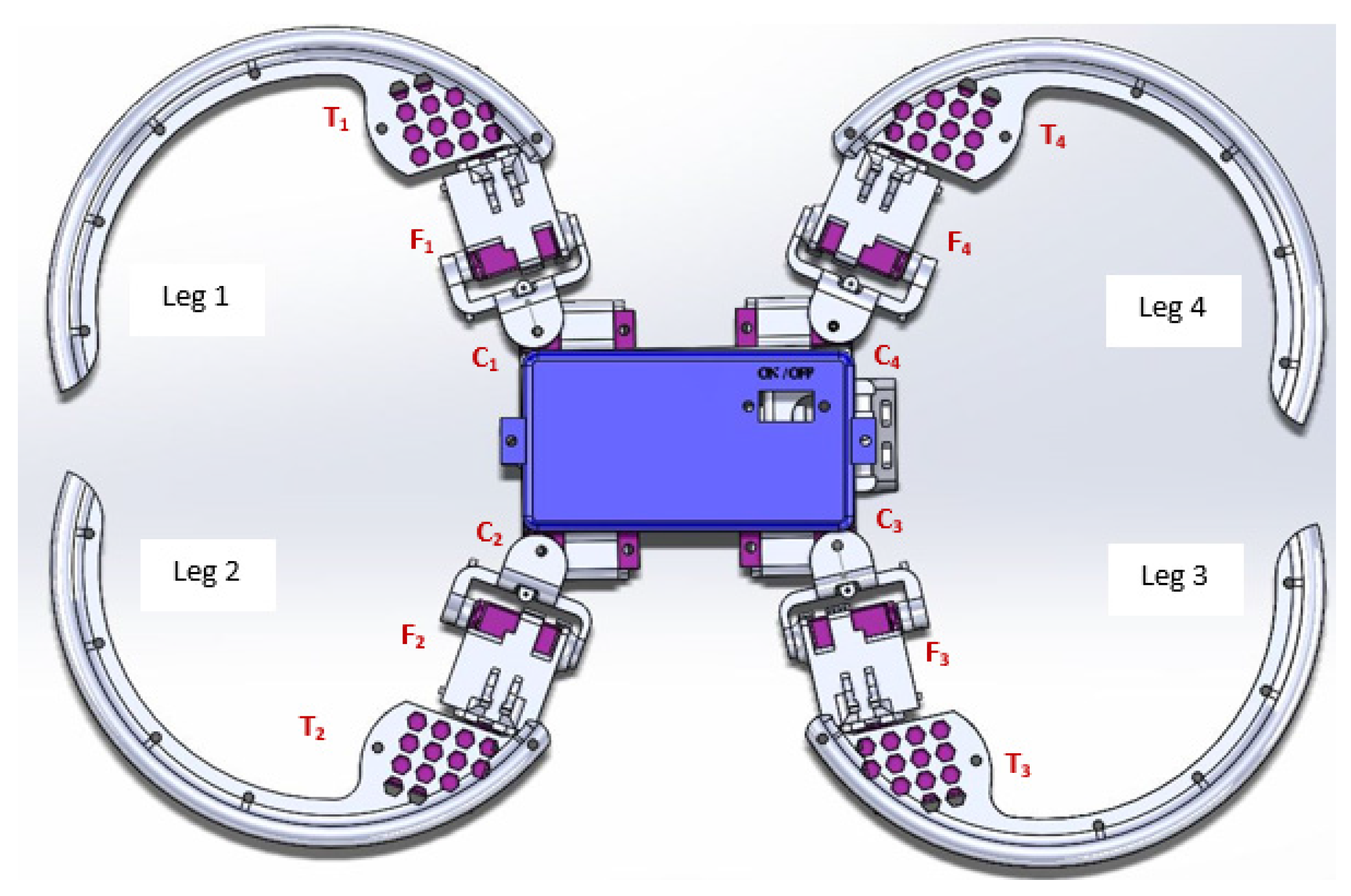
An extended set of locomotion and behavioral gaits has been synthesized from an exhaustive study of gaits in Cebrennus Rechenbergi spiders. Modeling, simulation, and synthesis were accomplished with real hardware. Our fault diagnostics experiments included nine distinct locomotion gaits, including forward, backward, right-turn, left-turn, curve-left, curve-right, shift-right, shift-left, and rolling locomotion modes. The outer body of the robot is made from Polylactic acid (PLA) plastic used in three-dimensional (3D) printing. The robot has four legs, with each leg containing three servo motors, which provide it with three degrees of freedom to realize crawling and rolling motions. To reduce the weight and size of the robot, a motor with a dimension of 21.5 mm × 11.5 mm × 21.5 mm and weight of 11.5 g is chosen. In total, the robot consists of 12 JR ES376 servo motors, each requiring a voltage of 4.8 V. A Pololu Maestro servo controller is used to interface the 12 servo motors via a microcontroller, which provides the user with an option to control the motors. Figure 1 presents the Computer Aided Design (CAD) model of our Scorpio robot with actuator details.

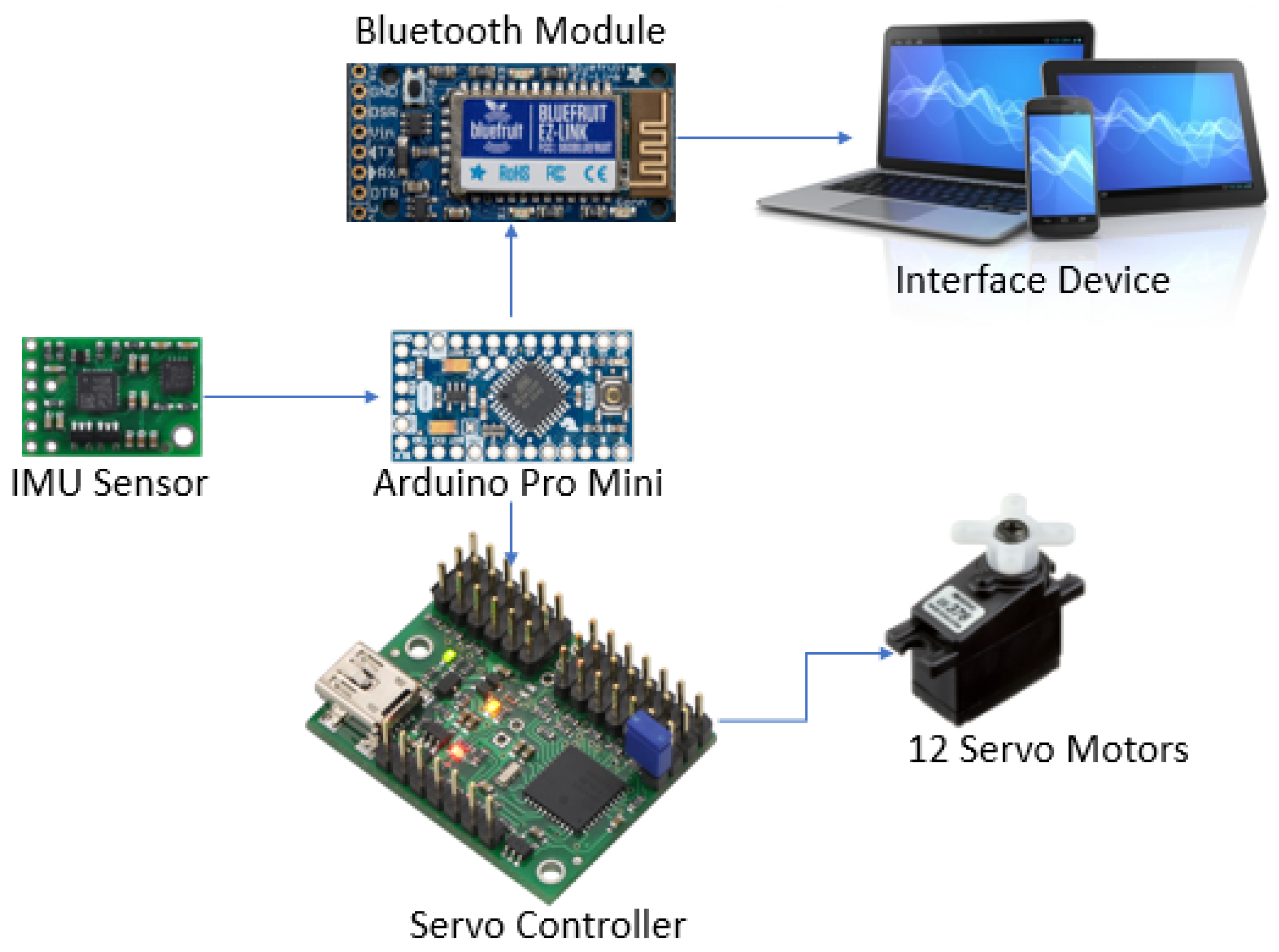
In addition to the actuators that enable robot locomotion, the platform is also equipped with an IMU sensor and a central microcontroller. The IMU sensor used is a Pololu MinIMU-9 v3 (which contains an L3GD20H 3-axis gyro), a LSM303D three-axis accelerometer, and a three-axis magnetometer. The IMU sensor provides the rotational and translational data so that the robot can enable the user to detect any anomalies in robot locomotion gait. The specific IMU sensor was chosen due to the smaller footprint and size constraints of the Scorpio platform. An Arduino pro-mini based on ATmega328, which requires about 5 to 12 V, is used as the central microcontroller. The hardware specifications of our Scorpio robot are detailed in

Table 1. Hardware Specification of Scorpio Robot.

Hardware Components	Specifications
Central Controller	Arduino Mini Pro with ATmega 328
Servo Motor	JR ES376
Servo Controller	Pololu maestro Servo controller
IMU	Pololu MinIMU-9 v3
Outer body	Polylactic acid or polylactide (PLA)
Power supply	Li-Po 1200mah
Communication Unit	Bluefruit EZ-Link

.

The IMU sensor constantly communicates with the accelerometer and the gyroscope via update messages to the Arduino pro mini microcontroller. The Arduino controller delivers the output control commands to the servo controller through a serial communication protocol. The Pololu Maestro servo controller can control up to 18 servo motors. The robot can be operated by a wireless device equipped with an onboard Bluefruit EZ-Link transceiver. The overall system architecture of the Scorpio robot is shown in Figure 2.

2.1. Crawling Locomotion

The crawling locomotion gait is achieved by the simultaneous rotation of two motors about the roll and yaw axis. In the forward or backward crawling motion, the fem motor is used to lift the leg and provide the roll movement. The Cox motor is then used to push the leg forward or backwards and provide a yaw movement. To crawl right, the fem motor is used to instigate the roll movement. The Cox motor will move the leg in the clockwise direction; whereas, in the case of a crawl left, the Cox motor will be moving the leg in the anti-clockwise direction. Similarly, a set of eight crawling gaits has been developed for our Scorpio robot. Only the Cox and fem motors are used in all the crawling locomotion gaits. The maximum crawling speed of the considered Scorpio robot is 15 cm/s.

2.2. Rolling Locomotion

Crawling is used as a default locomotion gait in our Scorpio robot. The robot must transform from a crawling position to a rolling position to achieve rolling locomotion. Rolling locomotion offers superior locomotion performance while traversing over flat terrain, slopes, and staircases. The transformation is made by shifting leg 3 and leg 4 upside-down and forming a circle along with leg 1 and leg 2. Along with the fem and Cox motors, T₃ and T₄ are also used to turn leg 3 and leg 4 to achieve the rolling position. In the rolling position, two legs will be in contact with the ground at any point. The motor on these two legs will be actuated to achieve forward or backward rolling locomotion. Once the robot has attained one-half of the rolling motion, the other two legs will be in contact with the ground, which will be reset to achieve the next half of the rolling motion. Only the fem motors are used to achieve the rolling locomotion. Figure 3 presents the crawling and rolling morphologies of our Scorpio robot. The maximum rolling speed of the considered Scorpio robot is 120 cm/s.

3. Feature Extraction

To perform fault classification, we need statistical features that standardize the characteristics of the robot in case of faulty and non-faulty conditions. In this paper, we use gyroscope and accelerometer readings from an IMU sensor. From the obtained results, we extract the mean, standard deviation, variance, root-mean-square level, peak-to-peak, root sum of squares level, and maximum value. In the context of fault classification in Scorpio gaits, the use of statistical methods for feature extraction greatly reduces the dimensionality of the original IMU sensor data features. The IMU data used for this study included a total of seven values; namely, three axes for accelerometer, three axes for gyroscope, and one axis for magnetometer.

(a)

Mean: Mean is the measure of the average of an IMU data set at a given instance. The mean of each IMU data set is calculated and used as one of the statistical features.

$$\mathrm{Mean}=\frac{{{\displaystyle \sum }}_{\mathrm{i}=1}^{\mathrm{N}}{\mathrm{x}}_{\mathrm{i}}}{\mathrm{N}}$$

(1)

where,

• x represents the IMU data for an instance
• N accounts for the number of IMU data in that instance.
• In our case, N = 7.

(b)

Standard deviation: Standard deviation is the measure of how spread out each IMU data point is from each other. This measure will also be able to gauge the difference between each IMU data point from its mean. This step calculates the standard deviation of IMU data obtained from each of data collection.

$$\mathrm{Standard}\mathrm{deviation}=\sqrt{\frac{1}{\mathrm{N}}{{\displaystyle \sum }}_{\mathrm{i}=1}^{\mathrm{N}}{\left({\mathrm{x}}_{\mathrm{i}}-\mathsf{\mu }\right)}^2}$$

(2)

where,

• µ is the mean of the IMU data for an instance
• x represents the IMU data for an instance, and N = 7.

(c)

Variance: This measure represents the variance of the IMU data at a given instance. It is the squared standard deviation of the mean IMU data.

$$\mathrm{Variance}=\frac{1}{\mathrm{N}}{{\displaystyle \sum }}_{\mathrm{i}=1}^{\mathrm{N}}{\left({\mathrm{x}}_{\mathrm{i}}-\mathsf{\mu }\right)}^2$$

(3)

where,

• µ is the mean of the IMU data for an instance
• x represents the IMU data for an instance, and N = 7.

(d)

Root Mean Square: Root Mean Square is also referred to as quadratic mean and is the square root of the arithmetic mean of the squared sample IMU data. It represents the magnitude or the typical size of IMU data for each data collection.

$$\mathrm{Root}\mathrm{Mean}\mathrm{Square}=\sqrt{\frac{{{\displaystyle \sum }}_{\mathrm{i}=1}^{\mathrm{N}}{\left({\mathrm{x}}_{\mathrm{i}}\right)}^2}{\mathrm{N}}}$$

(4)

where,

• x represents the IMU data for an instance, and N = 7.

(e)

Peak-to-peak value: The peak-to-peak value calculates the difference between the maximum IMU value and the minimum IMU value at a given instance. The maximum IMU value at an instance is the crest, and the minimum IMU value at an instance is the trough.

Peak to peak value = crest − trough

(5)

(f)

Root sum of squares level: The root sum of squares is calculated by taking the square root of the sum of the squared IMU data obtained for a given instance.

$$\mathrm{Root}\mathrm{sum}\mathrm{of}\mathrm{squares}\mathrm{level}=\sqrt{{{\displaystyle \sum }}_{\mathrm{i}=1}^{\mathrm{N}}|{\mathrm{x}}_{\mathrm{i}}{|}^2}$$

(6)

where,

• x represents the IMU data for an instance, and N = 7.

(g)

Maximum Value: This feature represents the highest value of the data obtained from IMU at a single instance.

(h)

Sum: This feature adds up all the IMU data obtained for a given instance.

$$\mathrm{Sum}={{\displaystyle \sum }}_{\mathrm{i}=1}^{\mathrm{N}}{\mathrm{x}}_{\mathrm{i}}$$

(7)

where,

• x represents the IMU data for an instance, and N = 7.

4. Support Vector Machine (SVM)

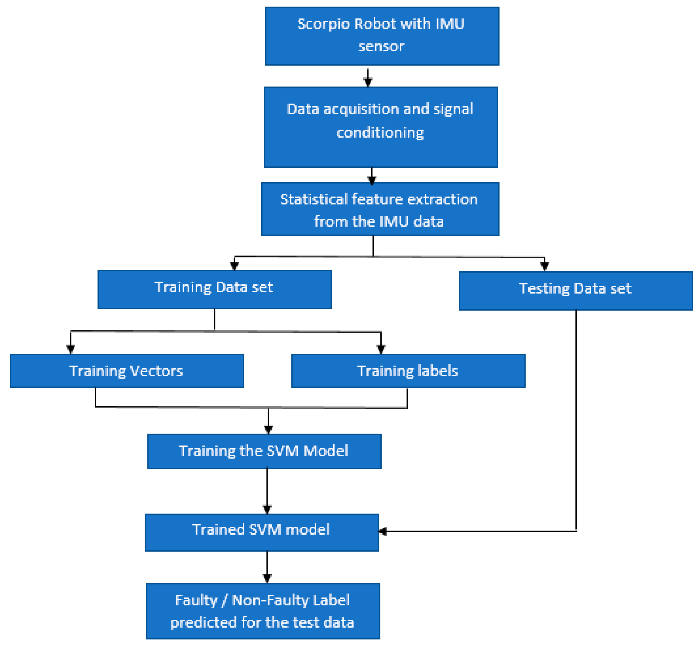
Once the statistical features are extracted from the IMU data, the next step is to use the features to generate a classification strategy for the data. Support Vector Machines (SVM) are viewed as one of the most accurate classification algorithms used in a supervised learning method of machine learning. In this paper, we used SVM to implement a fault diagnosis algorithm. An MATLAB-based program was developed using the Library of SVM (LIBSVM) package to implement SVM. LIBSVM requires the user to test the training vectors and training labels before the classifier is used to classify the test data. To obtain the training and testing dataset, the set of features obtained from the last few cycles is used as testing data, while the remaining data is used as training data. In addition, we also created a training label that indicates the true class of the training data in the same sequence. The flowchart in Figure 4 shows our fault classification process.

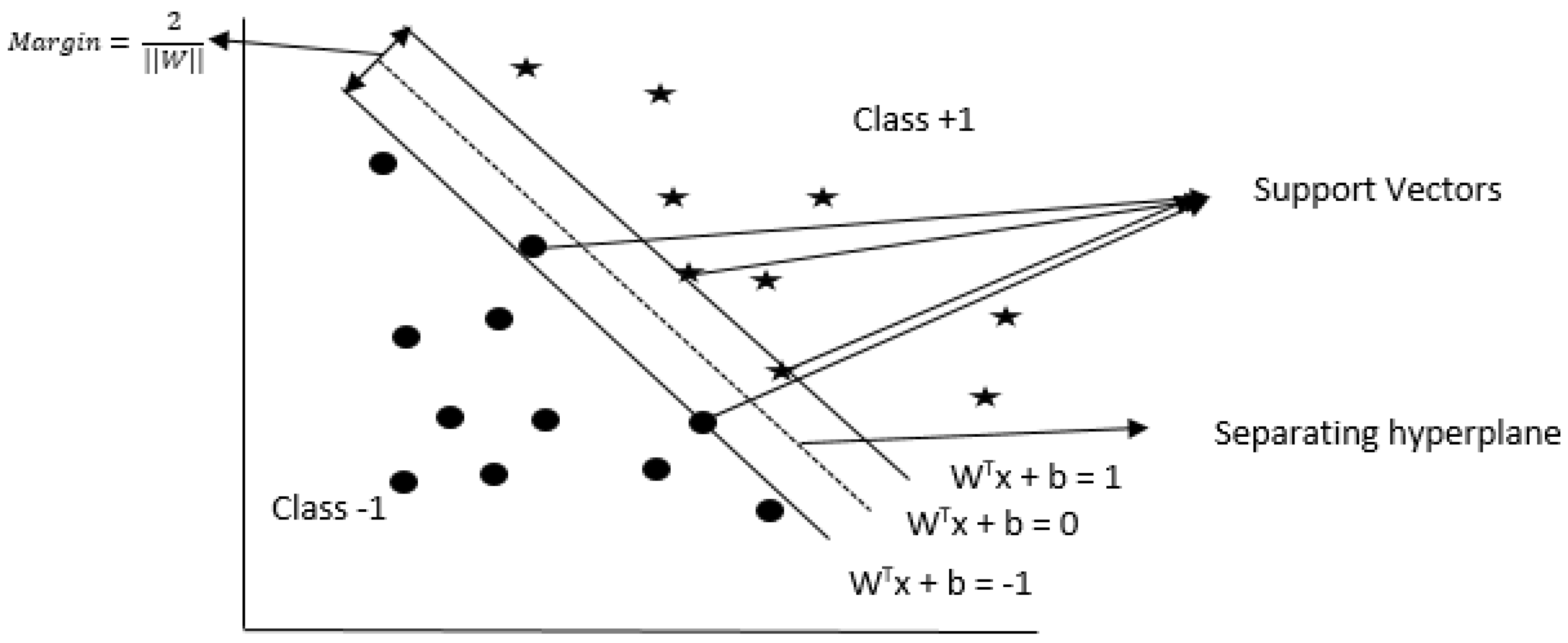
The goal of a support vector machine is to determine a hyperplane that separates data from two different classes. Figure 5 presents the standard support vector machine classifier. There can be multiple correct solutions for a single classification problem. An optimal solution for a classification problem using SVM is a hyperplane that separates the data from two different classes without error. This hyperplane must also have a maximum separation margin, from the closest training data, for each class. Such a hyperplane is called a maximum-margin hyperplane. This maximum separation margin between the two classes will ensure that the generalization error, when evaluated via testing data, is minimal, which in turn provides the classifier with improved accuracy. The training data may be linearly separable, or they could also be nonlinear. To make the classification easier and to minimize error, the training data is mapped into a higher dimensional space, where then the hyperplane is constructed in the higher dimensional space. To build an optimal separating hyperplane, two parallel hyperplanes are constructed, which will separate the training data of two classes. These two parallel hyperplanes are called bounding planes. The area between the two hyperplanes is called a margin. The final separating hyperplane should lie in the margin area, i.e., the area between the two parallel hyperplanes. The two parallel hyperplanes will contain some training data points lying on them, and these training data points, which are called support vectors, will be useful in constructing the final separating hyperplane.

Let us consider a two-class classification problem. We consider a set of training data in the following format:

 (xi, yi)

where i = 1,2,….n. n is the number of samples.

x_i is the training data set, and y_i is the label for the ith training data.

x_i ϵ Rⁿ and y_i ϵ {+1, −1}

The space between the two bounding planes is called a margin, and it is estimated to be $\frac{2}{\left|\left|W\right|\right|}$.

The SVM constructs a hyperplane that separates the two classes into +1 and −1. The equation of the hyperplane is characterized by

W^Tx + b = 0.

(8)

The classification is done using the following strategy.

X_i belongs to class +1 if W^Tx + b >0.

X_i belongs to class −1 if W^Tx + b <0.

In addition to this, we can also check if the classification is valid by using the following constraints. A proper classification must satisfy

y(w^Tx + b) ≥1.

(9)

In this paper, we have used two types of SVM: C-Support Vector Classification (c-SVC) and v-Support Vector Classification (v-SVC).

c-Support Vector Classification (c-SVC):

In c-SVC, C is the regularization parameter. The value c ranges from zero to infinity. Given a two-class classification problem (x_i, y_i) [23], where x_i is the training data, x_i ϵ Rⁿ for i = 1,2,…l, y_i, is the training label, and y_i ϵ {+1, −1} for all y ϵ R^l, c-SVC solves the following primal optimization problem

$$\begin{array}{c}\min \\ \mathrm{w},\mathrm{b},\mathsf{\xi }\end{array}\frac{1}{2}{\mathrm{w}}^{\mathrm{T}}\mathrm{w}+\mathrm{C}{{\displaystyle \sum }}_{\mathrm{i}=1}^{\mathrm{l}}{\mathsf{\xi }}_{\mathrm{i}}$$

(10)

subject to y_i(w^Tφ(x_i) + b) ≥ 1 − ξ_i and ξ_i ≥0.

The training data is x_i is mapped into a higher dimensional space by φ(x_i). This is done to provide a good classification in the case of nonlinear training data. We also need to solve the following dual problem.

$$\begin{array}{c}\min \\ \mathsf{\alpha }\end{array}\frac{1}{2}{\mathsf{\alpha }}^{\mathrm{T}}\mathrm{Q}\mathsf{\alpha }-{\mathrm{e}}^{\mathrm{T}}\mathsf{\alpha }$$

(11)

subject to y^T α = 0 and 0 ≤ α_i ≤ C.

Where e = [$\begin{array}{ccc}1,& \dots & ,1\end{array}$]

Q is a positive semidefinite matrix, and Q_ij = y_iy_jK(x_i, x_j).

The decision function obtained is characterized by

$$\mathrm{sgn}({\mathrm{w}}^{\mathrm{T}}\mathsf{\phi }(\mathrm{x})+\mathrm{b})=\mathrm{sgn}({{\displaystyle \sum }}_{\mathrm{i}=1}^{\mathrm{l}}{\mathrm{y}}_{\mathrm{i}}{\mathsf{\alpha }}_{\mathrm{i}}\mathrm{K}({\mathrm{x}}_{\mathrm{i}},\mathrm{x})+\mathrm{b})$$

(12)

v-Support Vector Classification (v-SVC):

In this Support vector classification, the variable v is taken as the regularization parameter, and it ranges from 0 to 1. Given a two-class classification problem (x_i, y_i) where x_i is the training data and x_i ϵ Rⁿ, i = 1,2,…l. y_i is the training label and y_i ϵ {+1, −1}, y ϵ R^l, v-SVC solves the following primal optimization problem

$$\begin{array}{c}\min \\ \mathrm{w},\mathrm{b},\mathsf{\xi },\mathsf{\rho }\end{array}\frac{1}{2}{\mathrm{w}}^{\mathrm{T}}\mathrm{w}-\mathrm{v}\mathsf{\rho }+\frac{1}{\mathrm{l}}{{\displaystyle \sum }}_{\mathrm{i}=1}^{\mathrm{l}}{\mathsf{\xi }}_{\mathrm{i}}$$

(13)

subject to y_i(w^Tφ(x_i) + b) ≥ ρ − ξ_i and ξ_i ≥0, ρ ≥0.

The dual problem in v-SVC is

$$\begin{array}{c}\min \\ \mathsf{\alpha }\end{array}\frac{1}{2}{\mathsf{\alpha }}^{\mathrm{T}}\mathrm{Q}\mathsf{\alpha }$$

(14)

subject to y^T α = 0, 0 ≤ α_i ≤ 1/l and e^T α ≥ v.

where Q_ij = y_i y_j K(x_i, x_j).

The final decision function is

$$\mathrm{sgn}({{\displaystyle \sum }}_{\mathrm{i}=1}^{\mathrm{l}}{\mathrm{y}}_{\mathrm{i}}{\mathsf{\alpha }}_{\mathrm{i}}\mathrm{K}\left({\mathrm{x}}_{\mathrm{i}},\mathrm{x}\right)+\mathrm{b})$$

(15)

In addition to using two different types of SVM, we have used two different kernels for each type of SVM. The two kernels are the linear and radial basis function. The linear kernel is optimal in cases when the training and testing data are linearly separable. The data are linearly separable if a single decision boundary line provides the necessary separation for classifying the data.

The linear kernel is characterized by

K(x_i, x_j) = x_i^Tx_j.

(16)

If the data is nonlinear, then the radial basis function kernel is a better option. This kernel maps the data into a higher dimensional space; thus, provides a better classification for nonlinear data than the linear kernel. The radial basis function kernel is characterized by

K(x_i, x_j) = exp(−ϒ || x_i − x_j ||²), ϒ >0.

(17)

5. Experimental Setup

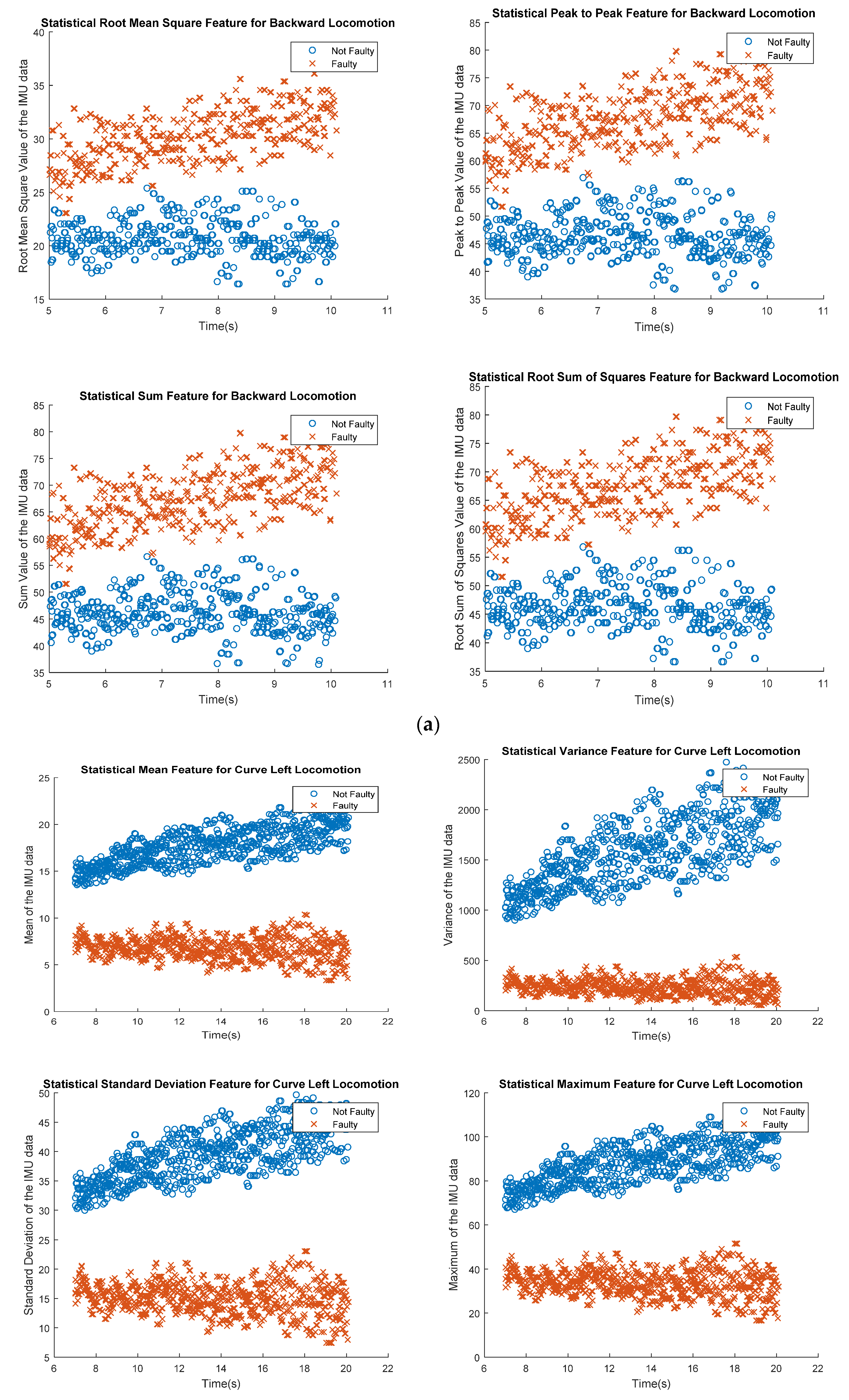
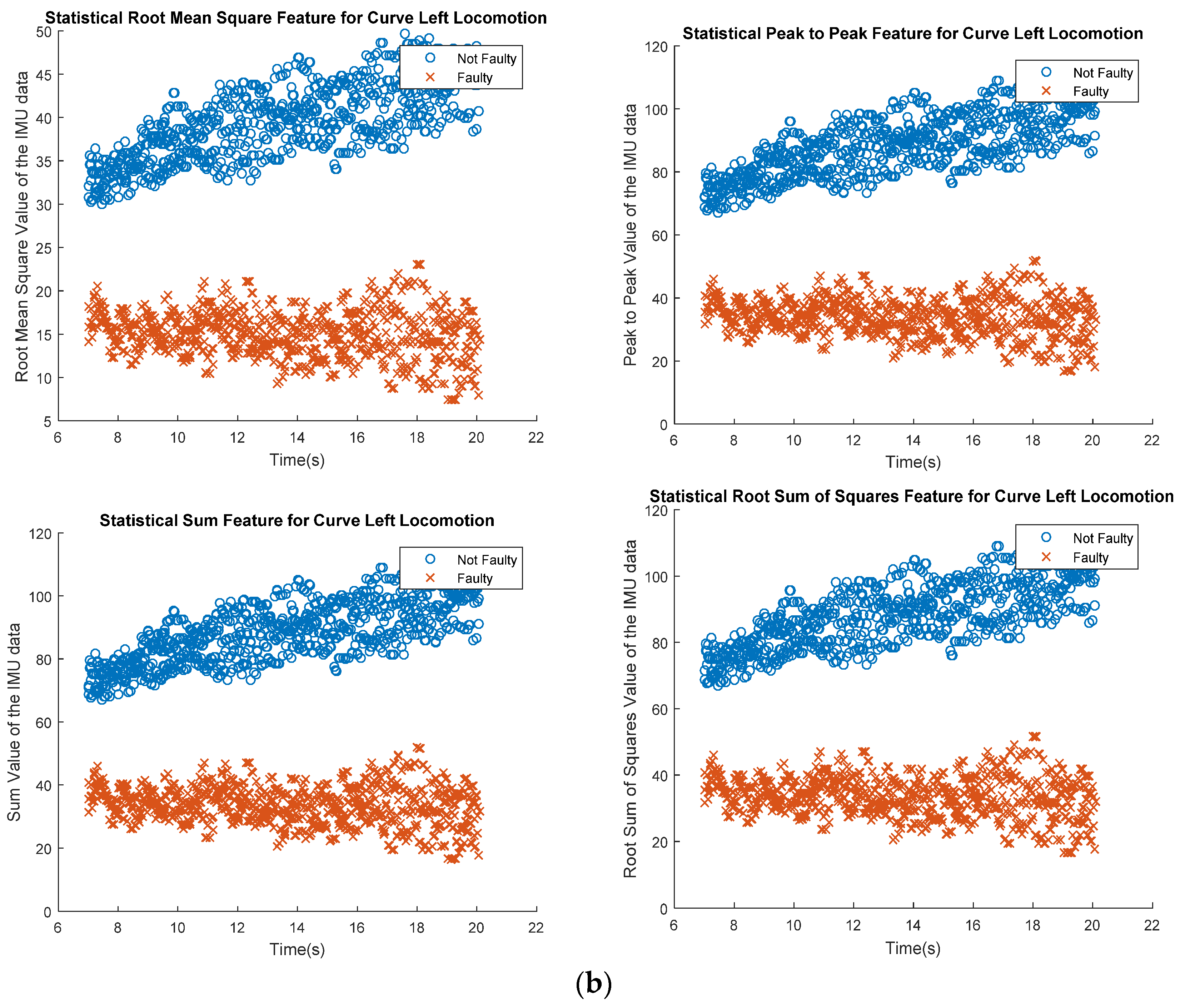
The experiment conducted in this paper uses statistical features that provide critical information needed to classify between faulty and non-faulty locomotion modes of our Scorpio robot. The nine most commonly used gaits in our Scorpio robot were chosen based on a set of pre-defined urban reconnaissance use cases. The identified gaits were tested across three different speeds identified for the same set of use cases. The IMU data is obtained for all nine gaits and all three speeds. When the program first starts running, it takes some readings to establish a baseline orientation, during which it expects both the roll and the pitch of the sensors to be zero. After performing the startup routine, the program constantly takes readings from the gyro, accelerometer, and magnetometer, and calculates an estimate of the robot’s data. The speed is varied by changing the degree of rotation per period in the servo motor. We used a total of eight statistical features, listed in Section 3, to perform the fault classification. Scatter plots illustrating the statistical features obtained from the IMU data, for backward locomotion gait at a speed of three degrees per period, are shown in Figure 6a, and curve left locomotion at a speed of six degrees per period is shown in Figure 6b.

The plot in Figure 6 illustrates the sample training sets used for fault classification. The plot denotes a clear separation between the faulty and non-faulty classes. The SVM classifier, when trained with the training data obtained from each gait, provides a useful fault classification for the corresponding locomotion gait. For calibration purposes, and due to the diverse nature of the locomotion gaits considered in this study, the feature sampling of IMU data were done separately from each locomotion gait. For example, in the backwards locomotion gait shown in Figure 6a, the IMU data were sampled in a period between 5s and 10 s, whereas for the curve left locomotion gait, the IMU data were sampled in a period between 7s and 20 s. We ensured that the IMU data, sampled for both faulty and non-faulty classes, were collected during the same period, which accounts for the calibration. In all gaits, except rolling, the faulty IMU data, used as training and testing classes, was obtained by deactivating the following motors: C₂ (Back-Left Cox), C₃ (Back-Right Cox), C₄ (Front-Right Cox). To consider the rolling motion, the fault data is obtained by simulating a disturbance in two of the fem motors, F₁ (Front-Left Fem) and F₄ (Front-Right Fem). Each disturbance is sufficiently large enough to prevent rolling motion. These faults were particularly considered for this study due their high degree of occurrence within the considered use cases. Future work is set to expand the scope of the faults considered for the study. The non-faulty IMU data are obtained when all motors, across the nine locomotion modes, are working properly.

6. Results and Discussions

The classification is carried out using MATLAB and the Library of SVM support package for each locomotion gait. The number of training and testing samples varied by gait and speed. The accuracy obtained from the SVM classification, across all nine locomotion gaits and three different speeds, is provided in

Table 2. Performance of the SVM classifier across nine locomotion gaits of the Scorpio robot.

Type of Locomotion Gaits		c-SVC 1		v-SVC 2
		Linear Kernel	Radial Basis Function Kernel	Linear Kernel	Radial Basis Function Kernel
Rolling	3 degree/period	100%	100%	100%	100%
	6 degree/period	92.44%	95.93%	100%	97.67%
	12 degree/period	95.29%	94.11%	96.47%	92.94%
Forward	3 degree/period	98.25%	97.09%	97.09%	95.93%
	6 degree/period	100%	100%	100%	100%
	12 degree/period	100%	100%	100%	100%
Backward	3 degree/period	100%	100%	99.41%	100%
	6 degree/period	100%	97.62%	100%	100%
	12 degree/period	100%	100%	100%	100%
Right Turn	3 degree/period	98.30%	98.72%	98.30%	98.30%
	6 degree/period	100%	97.04%	100%	94.09%
	12 degree/period	91.66%	92.26%	95.23%	91.66%
Left Turn	3 degree/period	100%	100%	100%	100%
	6 degree/period	100%	100%	100%	100%
	12 degree/period	95.90%	96.72%	95.90%	95.08%
Curve Right	3 degree/period	100%	98.88%	98.51%	98.14%
	6 degree/period	99.40%	95.83%	97.61%	100%
	12 degree/period	100%	100%	100%	95.23%
Curve Left	3 degree/period	100%	100%	100%	99.77%
	6 degree/period	100%	100%	100%	95.90%
	12 degree/period	100%	98.32%	100%	98.32%
Shift Right	3 degree/period	100%	100%	100%	100%
	6 degree/period	100%	100%	98.83%	98.83%
	12 degree/period	91.56%	92.77%	93.97%	95.78%
Shift Left	3 degree/period	100%	100%	99.50%	99.50%
	6 degree/period	98.88%	98.14%	92.93%	93.68%
	12 degree/period	100%	100%	92.57%	100%

¹ c-SVC: C-Support Vector Classification; ² v-SVC v-Support Vector Classification.

.

The classification is done for both c-SVC and v-SVC classifiers using a linear and an RBF kernel. The overall accuracy of each classifier is provided in

Table 3. Overall accuracy of the four classifiers.

Classifier Type		Overall Accuracy (%)
c-SVC	Linear Kernel	98.5823%
	Radial Basis Function Kernel	98.2774%
v-SVC	Linear Kernel	98.3849%
	Radial Basis Function Kernel	97.8109%

.

The linear kernel in the c-SVC classifier yields the highest overall accuracy, which is 98.5823%. The reason for such a high accuracy is that most of the statistical features used are linearly separable, i.e., linear in nature. We observe that the linear kernel, in both the c-SVC and v-SVC classifiers, yields a better accuracy than the corresponding RBF kernel. In machine learning, the performance of the classifier is often evaluated by analyzing a confusion matrix, which provides every possible result in tabular form: true positives, true negatives, false positives, and false negatives. In this work, we get a 2 × 2 confusion matrix that indicates the correct classifications and misclassification of the classifier of interest. The column indicates the instance in the predicted class, while the row indicates the instance in the original class. The sum of diagonal elements indicates the number of correct classifications, and the sum of anti-diagonal elements indicates the number of misclassifications. The confusion matrix for our experimental cases is listed in

Table 4. Confusion matrix obtained for our fault classification experiments.

Type of Locomotion Gait		c-SVC		v-SVC
		Linear Kernel	Radial Basis Function Kernel	Linear Kernel	Radial Basis Function Kernel
Rolling	3 degree/period	$\left[\begin{array}{cc}50& 0\\ 0& 53\end{array}\right]$	$\left[\begin{array}{cc}50& 0\\ 0& 53\end{array}\right]$	$\left[\begin{array}{cc}50& 0\\ 0& 53\end{array}\right]$	$\left[\begin{array}{cc}50& 0\\ 0& 53\end{array}\right]$
	6 degree/period	$\left[\begin{array}{cc}85& 0\\ 13& 74\end{array}\right]$	$\left[\begin{array}{cc}78& 7\\ 0& 87\end{array}\right]$	$\left[\begin{array}{cc}85& 0\\ 0& 87\end{array}\right]$	$\left[\begin{array}{cc}81& 4\\ 0& 87\end{array}\right]$
	12 degree/period	$\left[\begin{array}{cc}84& 0\\ 8& 78\end{array}\right]$	$\left[\begin{array}{cc}78& 6\\ 4& 82\end{array}\right]$	$\left[\begin{array}{cc}84& 0\\ 6& 80\end{array}\right]$	$\left[\begin{array}{cc}78& 6\\ 6& 80\end{array}\right]$
Forward	3 degree/period	$\left[\begin{array}{cc}83& 3\\ 0& 86\end{array}\right]$	$\left[\begin{array}{cc}83& 3\\ 2& 84\end{array}\right]$	$\left[\begin{array}{cc}81& 5\\ 0& 86\end{array}\right]$	$\left[\begin{array}{cc}83& 3\\ 4& 82\end{array}\right]$
	6 degree/period	$\left[\begin{array}{cc}86& 0\\ 0& 85\end{array}\right]$	$\left[\begin{array}{cc}86& 0\\ 0& 85\end{array}\right]$	$\left[\begin{array}{cc}86& 0\\ 0& 85\end{array}\right]$	$\left[\begin{array}{cc}86& 0\\ 0& 85\end{array}\right]$
	12 degree/period	$\left[\begin{array}{cc}69& 0\\ 0& 68\end{array}\right]$	$\left[\begin{array}{cc}69& 0\\ 0& 68\end{array}\right]$	$\left[\begin{array}{cc}69& 0\\ 0& 68\end{array}\right]$	$\left[\begin{array}{cc}69& 0\\ 0& 68\end{array}\right]$
Backward	3 degree/period	$\left[\begin{array}{cc}86& 0\\ 0& 86\end{array}\right]$	$\left[\begin{array}{cc}86& 0\\ 0& 86\end{array}\right]$	$\left[\begin{array}{cc}85& 1\\ 0& 86\end{array}\right]$	$\left[\begin{array}{cc}86& 0\\ 0& 86\end{array}\right]$
	6 degree/period	$\left[\begin{array}{cc}126& 0\\ 0& 127\end{array}\right]$	$\left[\begin{array}{cc}120& 6\\ 0& 127\end{array}\right]$	$\left[\begin{array}{cc}126& 0\\ 0& 127\end{array}\right]$	$\left[\begin{array}{cc}126& 0\\ 0& 127\end{array}\right]$
	12 degree/period	$\left[\begin{array}{cc}85& 0\\ 0& 86\end{array}\right]$	$\left[\begin{array}{cc}85& 0\\ 0& 86\end{array}\right]$	$\left[\begin{array}{cc}85& 0\\ 0& 86\end{array}\right]$	$\left[\begin{array}{cc}85& 0\\ 0& 86\end{array}\right]$
Right Turn	3 degree/period	$\left[\begin{array}{cc}115& 4\\ 0& 117\end{array}\right]$	$\left[\begin{array}{cc}116& 3\\ 0& 117\end{array}\right]$	$\left[\begin{array}{cc}115& 4\\ 0& 117\end{array}\right]$	$\left[\begin{array}{cc}115& 4\\ 0& 117\end{array}\right]$
	6 degree/period	$\left[\begin{array}{cc}118& 0\\ 0& 119\end{array}\right]$	$\left[\begin{array}{cc}118& 0\\ 7& 112\end{array}\right]$	$\left[\begin{array}{cc}118& 0\\ 0& 119\end{array}\right]$	$\left[\begin{array}{cc}118& 0\\ 14& 105\end{array}\right]$
	12 degree/period	$\left[\begin{array}{cc}84& 0\\ 14& 70\end{array}\right]$	$\left[\begin{array}{cc}84& 0\\ 13& 71\end{array}\right]$	$\left[\begin{array}{cc}84& 0\\ 8& 76\end{array}\right]$	$\left[\begin{array}{cc}84& 0\\ 14& 70\end{array}\right]$
Left Turn	3 degree/period	$\left[\begin{array}{cc}100& 0\\ 0& 100\end{array}\right]$	$\left[\begin{array}{cc}100& 0\\ 0& 100\end{array}\right]$	$\left[\begin{array}{cc}100& 0\\ 0& 100\end{array}\right]$	$\left[\begin{array}{cc}100& 0\\ 0& 100\end{array}\right]$
	6 degree/period	$\left[\begin{array}{cc}85& 0\\ 0& 87\end{array}\right]$	$\left[\begin{array}{cc}85& 0\\ 0& 87\end{array}\right]$	$\left[\begin{array}{cc}85& 0\\ 0& 87\end{array}\right]$	$\left[\begin{array}{cc}85& 0\\ 0& 87\end{array}\right]$
	12 degree/period	$\left[\begin{array}{cc}55& 5\\ 0& 62\end{array}\right]$	$\left[\begin{array}{cc}56& 4\\ 0& 62\end{array}\right]$	$\left[\begin{array}{cc}55& 5\\ 0& 62\end{array}\right]$	$\left[\begin{array}{cc}54& 6\\ 0& 62\end{array}\right]$
Curve Right	3 degree/period	$\left[\begin{array}{cc}136& 0\\ 0& 134\end{array}\right]$	$\left[\begin{array}{cc}136& 0\\ 3& 131\end{array}\right]$	$\left[\begin{array}{cc}132& 4\\ 0& 134\end{array}\right]$	$\left[\begin{array}{cc}136& 0\\ 5& 129\end{array}\right]$
	6 degree/period	$\left[\begin{array}{cc}84& 0\\ 1& 83\end{array}\right]$	$\left[\begin{array}{cc}77& 7\\ 0& 84\end{array}\right]$	$\left[\begin{array}{cc}84& 0\\ 4& 80\end{array}\right]$	$\left[\begin{array}{cc}84& 0\\ 0& 84\end{array}\right]$
	12 degree/period	$\left[\begin{array}{cc}84& 0\\ 0& 84\end{array}\right]$	$\left[\begin{array}{cc}84& 0\\ 0& 84\end{array}\right]$	$\left[\begin{array}{cc}84& 0\\ 0& 84\end{array}\right]$	$\left[\begin{array}{cc}76& 8\\ 0& 84\end{array}\right]$
Curve Left	3 degree/period	$\left[\begin{array}{cc}223& 0\\ 0& 223\end{array}\right]$	$\left[\begin{array}{cc}223& 0\\ 0& 223\end{array}\right]$	$\left[\begin{array}{cc}223& 0\\ 0& 223\end{array}\right]$	$\left[\begin{array}{cc}222& 1\\ 0& 223\end{array}\right]$
	6 degree/period	$\left[\begin{array}{cc}220& 0\\ 0& 220\end{array}\right]$	$\left[\begin{array}{cc}220& 0\\ 0& 220\end{array}\right]$	$\left[\begin{array}{cc}220& 0\\ 0& 220\end{array}\right]$	$\left[\begin{array}{cc}202& 18\\ 0& 220\end{array}\right]$
	12 degree/period	$\left[\begin{array}{cc}119& 0\\ 0& 120\end{array}\right]$	$\left[\begin{array}{cc}119& 0\\ 4& 116\end{array}\right]$	$\left[\begin{array}{cc}119& 0\\ 0& 120\end{array}\right]$	$\left[\begin{array}{cc}119& 0\\ 4& 116\end{array}\right]$
Shift Right	3 degree/period	$\left[\begin{array}{cc}151& 0\\ 0& 150\end{array}\right]$	$\left[\begin{array}{cc}151& 0\\ 0& 150\end{array}\right]$	$\left[\begin{array}{cc}151& 0\\ 0& 150\end{array}\right]$	$\left[\begin{array}{cc}151& 0\\ 0& 150\end{array}\right]$
	6 degree/period	$\left[\begin{array}{cc}86& 0\\ 0& 86\end{array}\right]$	$\left[\begin{array}{cc}86& 0\\ 0& 86\end{array}\right]$	$\left[\begin{array}{cc}84& 2\\ 0& 86\end{array}\right]$	$\left[\begin{array}{cc}84& 2\\ 0& 86\end{array}\right]$
	12 degree/period	$\left[\begin{array}{cc}84& 0\\ 14& 68\end{array}\right]$	$\left[\begin{array}{cc}84& 0\\ 12& 70\end{array}\right]$	$\left[\begin{array}{cc}84& 0\\ 10& 72\end{array}\right]$	$\left[\begin{array}{cc}84& 0\\ 7& 75\end{array}\right]$
Shift Left	3 degree/period	$\left[\begin{array}{cc}200& 0\\ 0& 202\end{array}\right]$	$\left[\begin{array}{cc}200& 0\\ 0& 202\end{array}\right]$	$\left[\begin{array}{cc}198& 2\\ 0& 202\end{array}\right]$	$\left[\begin{array}{cc}200& 0\\ 2& 200\end{array}\right]$
	6 degree/period	$\left[\begin{array}{cc}131& 3\\ 0& 135\end{array}\right]$	$\left[\begin{array}{cc}131& 3\\ 2& 133\end{array}\right]$	$\left[\begin{array}{cc}115& 19\\ 0& 135\end{array}\right]$	$\left[\begin{array}{cc}132& 2\\ 15& 120\end{array}\right]$
	12 degree/period	$\left[\begin{array}{cc}100& 0\\ 0& 102\end{array}\right]$	$\left[\begin{array}{cc}100& 0\\ 0& 102\end{array}\right]$	$\left[\begin{array}{cc}85& 15\\ 0& 102\end{array}\right]$	$\left[\begin{array}{cc}100& 0\\ 0& 102\end{array}\right]$

.

7. Conclusions

With robots being expected to perform jobs autonomously, with minimal or no human intervention, there is a clear need for those robots to autonomously detect and recover from a fault. In this paper, we have presented a novel approach for fault diagnosis using a Support Vector Machine. We tested the method on a crawling–rolling reconfigurable robot named Scorpio. Specifically, we classify between faulty and non-faulty conditions across nine different locomotion gaits involving rolling as well as crawling modes over three different speeds. We extract statistical features including mean, standard deviation, variance, root mean square, peak-to-peak value, root sum of squares level, maximum value, and sum from the IMU data onboard the robot platform. The selected features were fed as input to an SVM for classification between faulty and non-faulty conditions. We tested the algorithm using two different types of SVM; namely, c-SVC and v-SVC, and their performances were compared in the context of fault diagnostics in our Scorpio robot. In addition to using two different types of SVM, we tested two different kernels in each type of SVM. The two kernels used are linear and radial basis function. The results indicate a classification accuracy of over 90% for all of the SVM-based approaches tested over the nine locomotion gaits at three different speeds. The overall accuracy of all four classifiers is above 97%. The linear kernel of c-SVC and v-SVC classifiers provide a better overall accuracy compared to the RBF kernel of c-SVC and v-SVC classifiers. Future work will focus on the integration of additional sensors to extend the scope of fault classification and to classify fault types beyond what is currently possible. A systematic dynamic model is being developed to predict the effects of a known set of common faults on Scorpio gaits. Future work would also include full comparison of outcomes from such a model and experimental data. Another aspect of future work would be to expand fault classification to a larger set of locomotion gaits and to include transformation and climbing locomotion gaits.