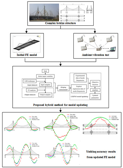
FE Model Updating on an In-Service Self-Anchored Suspension Bridge with Extra-Width Using Hybrid Method

Abstract

Nowadays, many more bridges with extra-width have been needed for vehicle throughput. In order to obtain a precise finite element (FE) model of those complex bridge structures, the practical hybrid updating method by integration of Gaussian mutation particle swarm optimization (GMPSO), Kriging meta-model and Latin hypercube sampling (LHS) was proposed. By demonstrating the efficiency and accuracy of the hybrid method through the model updating of a damaged simply supported beam, the proposed method was applied to the model updating of a self-anchored suspension bridge with extra-width which showed great necessity considering the results of ambient vibration test. The results of bridge model updating showed that both of the mode frequencies and shapes had relatively high agreement between the updated model and experimental structure. The successful model updating of this bridge fills in the blanks of model updating of a complex self-anchored suspension bridge. Moreover, the updating process enables other model updating issues for complex bridge structures.

1. Introduction

Self-anchored suspension bridges have attracted lots of attention from bridge engineers in recent years. Demonstrating both a relatively small size of the substructure and high adaptability to conditions of the site has resulted in the widespread use of this type of bridge structure [1]. Meanwhile, with the high increase of the requirement for vehicle throughput of bridge system, many more bridge structures with extra-width appear. For those large-scale and complex engineering structures, the evaluations of situation and behavior of bridges are usually based on finite element (FE) analysis [2,3,4,5,6]. FE analysis is one of the most effective methods used to solve those engineering problems, but due to the complexity of most existing engineering structures, we cannot get a precise model to reflect the behavior of the physical one [7,8]. Not only uncertainties in material and geometric parameters, but also stochastic factors in boundary and load conditions improve the inaccuracy between the FE model and physical one [9,10,11]. By identifying and modifying the uncertain parameters, model updating technique provides an effective way of yielding precise FE model to predict performance of physical structures, to which the engineers have drawn significant attention in recent years.

Generally, the methods of model updating can be classified into two categories. One is non-iterative method by directly modifying the element matrices of stiffness and mass with small perturbation [12,13], but the drawback is that those modified matrices lose their sparse character. Moreover, this modifying process can even result in negative values in matrices with no physical meaning. The other is iterative method by modifying the selected parameters after analysis of sensitivity like material module, density, moment of inertia, area of section, etc. This updating technique is common practice to transfer a model updating process into a bound-constrained optimization process. The objective function is set by the errors such as deflections, strains, accelerations, or mode frequencies between experimental and analytical models. The updating process is the process of minimizing the objective function by adjusting the selected parameters using the optimization methods [10,14,15].

Compared to traditional methods like Newton method or quasi-Newton method, which is easier to fall into local optimal solution in constrained optimization problems, methods based on artificial intelligence (AI)—such as genetic algorithm, simulated annealing algorithm, and swarm algorithm—have higher reliability and efficiency for nonlinear constrained optimization problems [11,16,17,18,19]. Among those AI algorithms, particle swarm optimization (PSO), first proposed by Kennedy and Eberhart [20,21,22], shows huge potential in solving practical optimization problems with less number of iteration to converge to the same or better result [23]. The basic idea of PSO is starting with a swarm of random particles in feasible regions and gradually approaching the optimal solution by information transferred among both particles and swarms. However, due to the lack of swarm diversity at the later stage of this algorithm, the ability of global convergence is weak as the algorithm may end prematurely. Hence, adjustments have been proposed to improve the property of PSO by some researchers with modifying the velocity and (or) position of particle. Gaussian mutation PSO (GMPSO), which gives the position of every particle a mutation of Gaussian white noise (GWN) disturbance to ensure the diversity of particle swarm, is proven to be an useful algorithm for solving nonlinear constrained optimization problems with rapid and steady global convergence [24].

When using GMPSO as a model updating method, numerous iterations would be performed during the optimization process. But the reality is that each iteration in GMPSO needs to re-run the FE package, which obviously increases the cost of computation, let alone the research object is a more complex or larger scale structure. To alleviate those problems, equivalent model, called the meta-model, is usually proposed to replace the initial FE model. The most commonly used meta-model method is response surface methodology (RSM), first proposed by Marwala [17], which establishes explicit function between selected parameters and eigenvalues whose relationship are properly complicated, implicit, and difficult to be expressed mathematically. Deng and Cai [11] utilized a second order polynomial response surface (RS) representing the relationship between selected parameters and structural responses, then the parameters were updated by genetic algorithm. This method was applied to model updating of a two-way bridge located in Louisiana. Ren et al. [25] presented an updating method based on polynomial RSM using uniform design and the proposed method was verified by a six-girder bridge. However, for higher order nonlinear relationship between parameters and responses, the polynomial RS cannot be applied. Instead, a more suitable meta-model—i.e., Kriging meta-model—is proposed. This meta-model, another type of RS, was originally developed by Krige in 1951 [26], which is first applied in area of mining and geo-statistics. After adding a stochastic process behind the polynomial part, the accuracy of the meta-model is improved significantly.

In this article, realizing the model updating of a self-anchored suspension bridge with extra-width, a practical model updating hybrid methodology by integration of GMPSO and Kriging meta-model is proposed and implemented. The architecture of the hybrid method consists of three main stages of analysis: (1) selecting reasonable samples of random parameters as input datasets using LHS and performing FE analyses with the input parameters to obtain output datasets; (2) formulating the Kriging meta-model based on input and output datasets; and (3) applying GMPSO as an optimization technique with an objective function set as errors between experimental value and Kriging model to yield the updated values of selected parameters. The accuracy of this hybrid method is first demonstrated through the analysis of model updating of a simply supported beam. Then the method is applied to model updating of Hunan Road Bridge, a self-anchored suspension bridge with extra-width in Shandong Province in China. Results show the proposed method can obtain reasonable values of updated parameters and show great efficiency and accuracy in model updating issues. This article is organized as follows. Section 2 presents the theory background of GMPSO method, Kriging meta-model method, Latin hypercube sampling, and the hybrid model updating method. Section 3 introduces the study example of model updating of a damaged simply supported beam. Section 4 describes the details model updating process of Hunan Road Bridge using the hybrid method and conclusions are made in Section 5.

2. Hybrid Model Updating Method

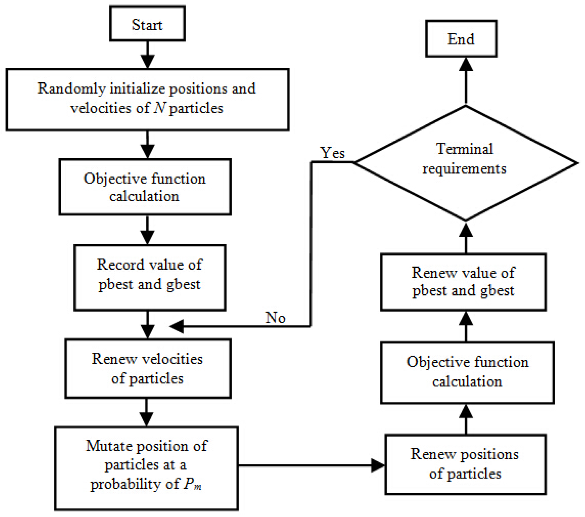
2.1. GMPSO

GMPSO is a stochastic global search algorithm based on adjustment of standard PSO. Supposing there are an amount of N random initialization particles with a d-dimensional searching space in which the position and velocity of particle i are $X_i=[x_{i1},x_{i2},\cdot \cdot \cdot ,x_{id}]$ and $V_i=[v_{i1},v_{i2},\cdot \cdot \cdot ,v_{id}]$, respectively. In every iteration process, particle i can yield two best solutions of the objective function, one is the personal best (pbest), $P_i=[p_{i1},p_{i2},\cdot \cdot \cdot ,p_{id}]$ and the other is the global best (gbest), $P_g=[p_{g1},p_{g2},\cdot \cdot \cdot ,p_{gd}]$. For a standard PSO, the particle i adjusts its velocity and position according to the following equations:

$$v_{ij}(t+1)=\omega v_{ij}\left(t\right)+c_1{r}_1[p_{ij}-x_{ij}(t\left)\right]+c_2{r}_2[p_{gj}-x_{ij}(t\left)\right]$$

(1)

$$x_{ij}(t+1)=x_{ij}\left(t\right)+v_{ij}(t+1)\times \Delta t$$

(2)

where i = 1, 2, …, N, j = 1, 2, …, d, ∆t = 1, t is the t-th iteration, w is inertia weight, c₁ and c₂ are positive learning coefficients, namely acceleration coefficients, r₁ and r₂ are random numbers uniformly distributed between 0 and 1. In the Equation (1) of subsequent velocity, the first part represents the inheritance of current state, the second part means self-cognition namely experiences and memories of itself which enables global search capability and the last part reflects group-cognition based on experiences of entire particles which improves the global search ability. As aforementioned, the drawback of standard PSO is the lack of swarm diversity at the later stage which influences the global convergence as the algorithm may end prematurely. Through introducing mutation of Gaussian white noise (GWN) disturbance for position of every particle at a probability, GMPSO apparently increases the diversity of particle swarm [23]. For a GMPSO algorithm, the position of particle i, $X_i=[x_{i1},x_{i2},\cdot \cdot \cdot ,x_{id}]$, is mutated by disturbance of GWN at a probability of P_m around the global best position before the adjustment of Equation (2). The value of P_m is generally between 0.05 and 0.15 and the mutation formula is as follows

$$x_{ij}=p_{gj}\times (0.5+\mathsf{\sigma })$$

(3)

where $\mathsf{\sigma }$ is a random number of GWN and the other meanings of items are like before.

The detail steps shown in Figure 1 are as follows:

• Randomly initializing positions and velocities of N particles and setting the values of serials of parameters such as w, c₁, c₂, d, P_m, maximum iteration number, and the upper and lower bounds of search space;
• Establishing the objective function, called fitness function and calculating its value of each particle. Recording each particle’s current position and function value in pbest in which the best position and best value are recorded in gbest;
• Renewing velocity of particles based on Equation (1);
• Mutating position of particles at a probability of Pm based on Equation (3);
• Renewing position of particles based on Equation (2);
• Calculating function value again and replacing pbest if the current value is better than the former one.
• Replacing gbest in the current pbest and gbest according to the best value.
• Quitting searching if the iteration number reaches the maximum one or accuracy meets the limitation, otherwise, returning to Step 3.

2.2. Latin Hypercube Sampling with Bounded Parameters

Reasonable computer experimental design is necessary for establishing explicit relationship between selected parameters and interested responses of FE model. The simplest method to generate the input data sample is random sampling, but a significant drawback of the method is the lack of guarantee that the chosen data covers the entire design space uniformly. To overcome this shortage, Latin hypercube sampling (LHS), instead of methods of orthogonal design, uniform design, etc., has simpler operation, smaller calculation, higher accuracy, and can rapidly generate samples with interested number of parameters and dimensions [1,27].

For uncertain but bounded parameters, supposing $X$ is a variable vector of d parameters $[x_1,x_2,\cdot \cdot \cdot ,x_d]$, ([l₁,u₁],[l₂,u₂],…,[l_d,u_d]) is the lower and upper boundary value of each parameter, N is the interested number of samples. The steps of the LHS method are as follows. Firstly, each parameter is divided into N equal parts according to its boundary, namely $[l_i,l_i+\frac{u_i-l_i}{N}]$ = P_1i < P_2i < … < P_Ni = $[l_i+\frac{u_i-l_i}{N}(N-1),u_i]$, i = 1, 2, …, d; Secondly, a N × d matrix S₁

$$S_1=\left[\begin{array}{cccc}{P}_{11}& P_{12}& \dots & P_{1d}\\ P_{21}& P_{22}& \dots & P_{2d}\\ ⋮& ⋮& \ddots & ⋮\\ P_{N1}& P_{N2}& \cdots & P_{Nd}\end{array}\right]$$

(4)

can be obtained in which every element is a small boundary; Thirdly, a matrix S₂ is transformed from matrix S₁ with elements at each column, namely P_1i, P_2i,…, P_Ni, arranging to be in random order; Then, a matrix S is transformed from matrix S₂ with elements chosen randomly in correlation small boundaries. In matrix S, each row represents one sample vector of d parameters.

2.3. Kriging Meta-Model

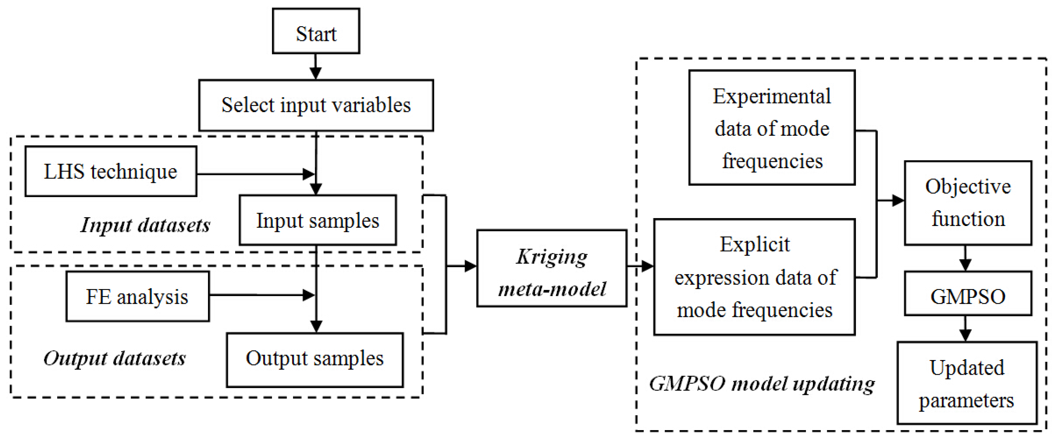
For a Kriging meta-model, supposing the unknown function is combined by a polynomial part and a stochastic process which provide a global model and localized departures respectively. The formula is as follows

$$y(X)=f^{\mathrm{T}}(X)\mathsf{\beta }+z(X)$$

(5)

where $X$ is variable vector of d parameters $[x_1\cdot \cdot \cdot x_d]$, for example, the ith vector of d parameters $X_i=[x_{i1}\cdot \cdot \cdot x_{id}]$; $y(X)$ is the response of FE model with parameter condition of $X$; $f^{\mathrm{T}}(X)$ is a vector of m polynomial functions, namely $f^{\mathrm{T}}(X)=[f_1(X)\cdot \cdot \cdot f_m(X)]$; $\mathsf{\beta }$ is a vector of m regression coefficients, $\mathsf{\beta }={[{\beta }_1\cdot \cdot \cdot {\beta }_m]}^{\mathrm{T}}$; $z(X)$ is a Gaussian stationary stochastic process with mean 0 and variance ${\mathsf{\sigma }}^2$. The covariance of arbitrary two elements in $z(X)$ is as follows

$$\mathbf{cov}(z(X_i)z(X_j))={\mathsf{\sigma }}^{2}R(X_i,X_j)={\mathsf{\sigma }}^2\exp (-{\displaystyle \sum _{k=1}^d{\mathsf{\theta }}_k|x_{i,k}}-x_{j,k}{|}^2)$$

(6)

where $R(X_i,X_j)$ is the spatial correlation of two samples which is usually implemented Gaussian function $\exp (-{\displaystyle \sum _{k=1}^d{\mathsf{\theta }}_k|x_{i,k}}-x_{j,k}{|}^2)$ as a core function because its calculation effect is the most welcome; ${\mathsf{\theta }}_k$ is coefficient with value over zero in computation of spatial correlation. Supposing there are N samples, the matrices of responses and polynomial values are $Y=[y(X_1)\cdot \cdot \cdot y(X_N)]$ and $F={[f^{\mathrm{T}}(X_1)\cdot \cdot \cdot f^{\mathrm{T}}(X_N)]}^{\mathrm{T}}$, respectively. The estimated values of $\mathsf{\beta }$ and ${\mathsf{\sigma }}^2$ are as follows

$$\widehat{\mathsf{\beta }}={(F^{\mathrm{T}}{R}^{-1}F)}^{-1}{F}^{\mathrm{T}}{R}^{-1}Y$$

(7)

$${\widehat{\mathsf{\sigma }}}^2=\frac{1}{N}{(Y-F\widehat{\mathsf{\beta }})}^{\mathrm{T}}{R}^{-1}(Y-F\widehat{\mathsf{\beta }})$$

(8)

where spatial correlation matrix

$$R=\left[\begin{array}{cccc}R(X_1,X_1)& R(X_1,X_2)& \dots & R(X_1,X_N)\\ R(X_2,X_1)& R(X_2,X_2)& \dots & R(X_2,X_N)\\ ⋮& ⋮& \ddots & ⋮\\ R(X_N,X_1)& R(X_N,X_2)& \cdots & R(X_N,X_N)\end{array}\right]$$

(9)

In above equations, before obtaining values of $\widehat{\mathsf{\beta }}$, ${\widehat{\mathsf{\sigma }}}^2$ and $R$ through Equations (7)–(9), ${\mathsf{\theta }}_1$,… and ${\mathsf{\theta }}_d$ should be known first. By implementing maximum likelihood estimation method, ${\mathsf{\theta }}_1$,… and ${\mathsf{\theta }}_d$ should be selected to get minimum value of expression below

$$\underset{{\mathsf{\theta }}_1>0,\mathrm{...},{\mathsf{\theta }}_d>0}{{\displaystyle \min }}\{\frac{1}{2}[N\ln ({\widehat{\mathsf{\sigma }}}^2)+\ln |R|]\}$$

(10)

where $\left|R\right|$ is determinant of matrix $R$, the optimal values of ${\mathsf{\theta }}_1$,… and ${\mathsf{\theta }}_d$ can be obtained by optimization method such as Genetic Algorithm (GA), Particle Swarm Optimization (PSO), etc. with an objective function of Equation (10). Once ${\mathsf{\theta }}_1$,… and ${\mathsf{\theta }}_d$ are determined, the best linear unbiased predicted value of interested performance is

$$\widehat{y}(X)=f^{\mathrm{T}}(X)\widehat{\mathsf{\beta }}+r^{\mathrm{T}}(X)\widehat{\mathsf{\alpha }}$$

(11)

where $r^{\mathrm{T}}(X)\widehat{\mathsf{\alpha }}=\widehat{z}(X)$ denotes interpolation of residuals of regression model $f^{\mathrm{T}}(X)\widehat{\mathsf{\beta }}$, vector $r^{\mathrm{T}}(X)=[R(X,X_1),R(X,X_2),\cdots ,R(X,X_N)]$, vector $\widehat{\mathsf{\alpha }}=R^{-1}(Y-F\widehat{\mathsf{\beta }})$.

2.4. Hybrid Method

The hybrid method is a combination of the aforementioned techniques that involves following processes illustrated in Figure 2.

• Applying LHS method to select reasonable samples of random parameters as input datasets;
• Performing a series of the FE analyses with the input parameters to obtain the interested mode frequencies of the structure as the output datasets;
• Determining the architecture of the Kriging meta-model, yielding its correlation coefficients with the input and output datasets with Equations (6)–(10) and extracting the explicit expression based on Equation (11);
• Applying GMPSO as an optimization technique with an objective function which is the sum of natural frequencies residuals between experimental value and Kriging model according to Figure 1;
• Yielding the updated values of parameters after several iterations.

To apply this hybrid method to solve model updating problem, a combined program based on both MATLAB-code and ANSYS-APDL is developed. The program is performed in modular form so that it can be easily used in other model updating of structures, which obviously facilitate practical application.

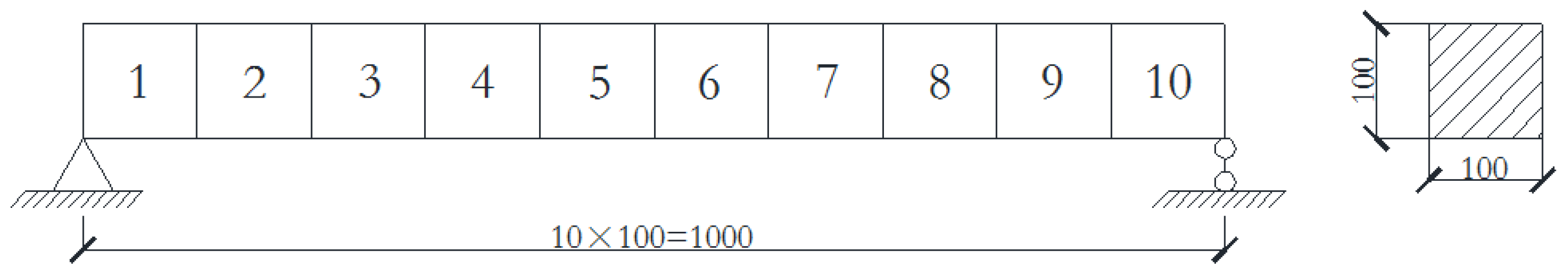
3. Case Study of a Damaged Simply Supported Beam

A damaged simply supported beam is selected as an example to demonstrate the efficiency and accuracy of the proposed hybrid method. The structure is a 10 m-span beam, shown in Figure 3, with a rectangle section of 1 × 1 m. The elastic module and density of material are 3.45 × 1010 Pa and 2600 kg/m³, respectively. The gravity acceleration is 9.806 m/s² and the damping ratio of beam is 0.05. BEAM 44 element is used to establish the FE model based on ANSYS (12.0, ANSYS Inc., Canonsburg, PA, USA) and the model consists of 11 nodes and 10 elements. To get the experimental data of mode frequencies, two damaged locations are assumed in this beam, of which the moment inertia of section in elements 3 and 8 reduce to 70% of original value, the aim of using the proposed method is yielding precise FE model which can reflect this damage. Ten parameters of ratio coefficients (real value/original value) of moment inertia of those 10 element sections in Figure 3 (for example, initial FE model with parameter vector of [1,1,1,1,1,1,1,1,1,1] and objective model with parameter vector of [1,1,0.7,1,1,1,1,0.7,1,1]) are selected as modified parameters. In this case study, both direct GMPSO and proposed hybrid method are implemented.

For direct GMPSO with a particle described as $X_i=[x_{i1},x_{i2},\cdot \cdot \cdot ,x_{i10}]$, the lower and upper boundary of each parameter is assumed to be 0.6 and 1.1, respectively. The amount of particles N is 60, the inertia weight w is 0.55, the learning coefficients c₁ and c₂ are both 2, the probability of P_m is set as 0.1 and the maximum iteration number is 60. Objective function is chosen as the sum of residuals of frequencies of first two vertical bending mode and first two transverse bending mode between FE value and experimental value. The modified parameters shown in

Table 1. Parameter values of updated and experimental model with different methods.

Parameter	1	2	3	4	5	6	7	8	9	10
Experimental model	1.000	1.000	0.700	1.000	1.000	1.000	1.000	0.700	1.000	1.000
Direct GMPSO	0.991	0.945	0.717	0.978	1.005	1.037	0.982	0.729	0.980	1.034
Hybrid method	1.025	1.016	0.735	0.932	0.932	1.078	1.008	0.668	0.968	0.993

are obtained and the frequency comparison of first 10 modes between the updated and experimental model are shown in

Table 2. The comparison between updated and experimental frequencies ¹.

Mode	Experimental Frequency/Hz	Updated Frequency/Hz		Difference/%
		Direct GMPSO	Hybrid Method	Direct GMPSO	Hybrid Method
1	15.39069	15.43708	15.31826	0.30	0.47
2	37.14974	37.25102	37.14082	0.27	0.02
3	52.36193	52.31448	52.41372	0.09	0.10
4	83.96296	83.96269	83.58468	0.00	0.45
5	96.36669	96.79726	96.11117	0.45	0.27
6	116.64350	116.43540	116.98770	0.18	0.30
7	144.77070	145.07480	144.88010	0.21	0.08
8	184.79670	186.12250	184.99380	0.72	0.11
9	223.79820	223.20420	223.93680	0.27	0.06
10	254.07320	255.31840	254.94600	0.49	0.34

¹ $\mathrm{Difference}=\frac{|\mathrm{Updated}\mathrm{Frequency}-\mathrm{Experimental}\mathrm{Frequency}|}{\mathrm{Experimental}\mathrm{Frequency}}\times 100\%$.

. Finally, this optimization process takes nearly five hours.

For the proposed hybrid method, the lower and upper boundary of each parameter is the same. Firstly, using LHS technique, 200 input samples of selected parameters are yielded. Secondly, after a series of FE analyses, output datasets, and mode frequencies of first two vertical bending modes and first two transverse bending modes, are obtained. This process needs a total time of approximately 400 s. Thirdly, the Kriging meta-model of each mode frequency represents the explicit expression between parameters and those frequencies which needs a total calculation time of 3140 s. Finally, GMPSO technique is introduced in the updating process with an objective function of the sum of the four frequencies residuals between explicit expression value and experimental value. 100 particles, 100 maximum iteration number, and other coefficients and objective functions chosen as the same as aforementioned are selected for the GMPSO algorithm. The final updated parameters shown in Table 1 are obtained after time of 3 s and the frequency comparison of first 10 modes between the updated model and experimental model is shown Table 2. The total model updating time of the proposed method is less than one hour, which is only 0.2 times of direct GMPSO.

In this case study, it can be seen that both direct GMPSO and the proposed hybrid method can get an approximate model of this damaged bridge, which means the damage in elements 3 and 8 are both identified. In Table 2, the differences of all the first ten mode frequencies between the updated and experimental model are below 1% which indicates the updated model reflects the damaged one very well. However, from the view of efficiency, the proposed hybrid method is better than direct GMPSO, being five times faster. It is evident that the results of direct GMPSO and hybrid method are highly consistent, which demonstrates that the proposed hybrid method is applicable to model updating of structures with multi-parameters. More importantly, the updating process can be performed more efficiently without losing accuracy.

4. Application to Model Updating of an In-Service Bridge with Extra-Width

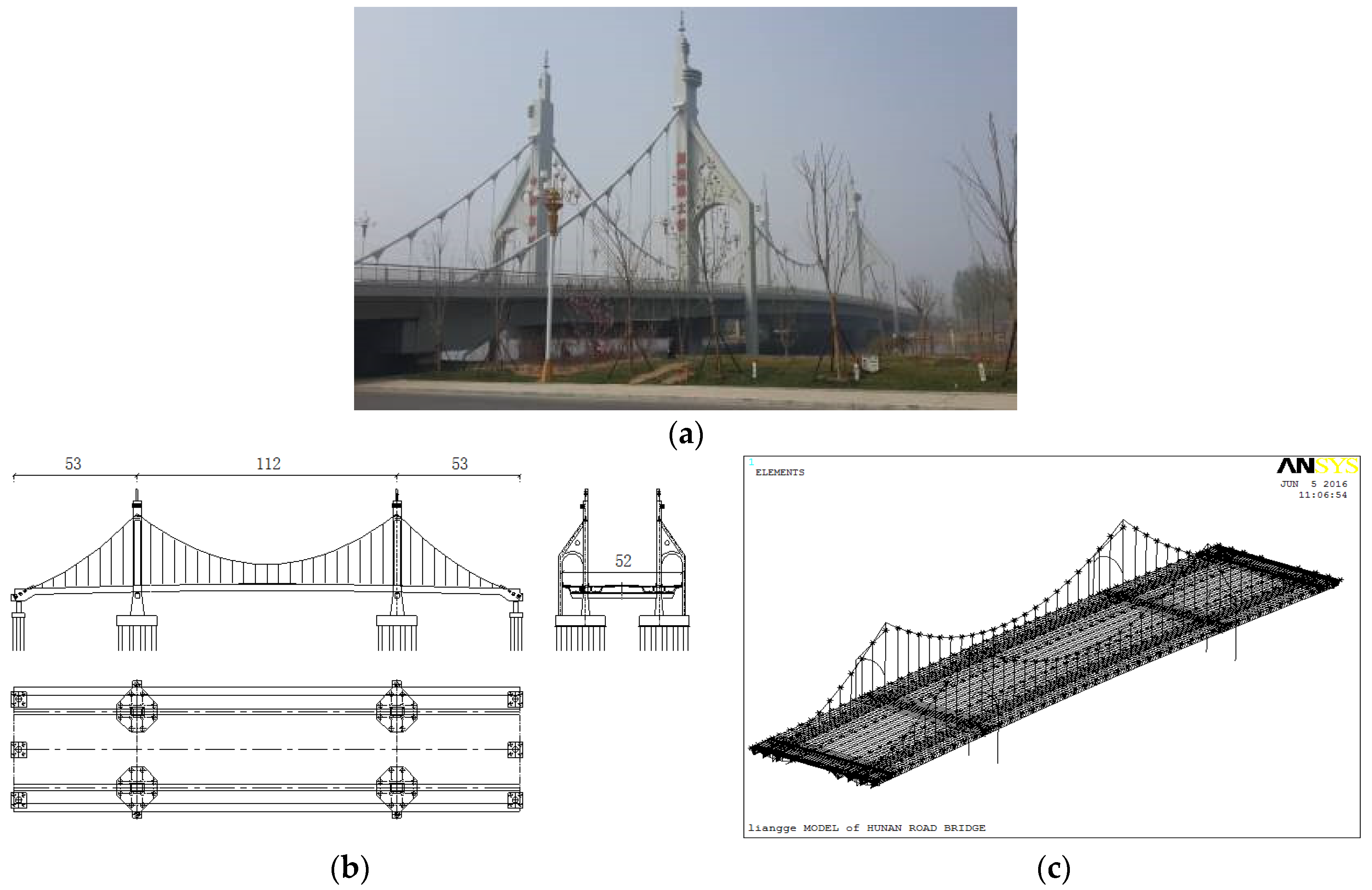
4.1. Description of Bridge Structure

The pre-stressed concrete bridge, Hunan Road Bridge in Liaocheng City of Shandong Province in China shown in Figure 4a, a self-anchored suspension bridge with double-tower and double-cable plane, has a span arrangement of 53 + 112 + 53 m and a total width of 52 m. The main girder with material of C50 concrete has a section of double-lateral box connected by transverse beams with a height of 2.8 m of standard section and a height from 4.3 to 5.6 m of sections in the region of the main cable anchorage. The tower is made of C40, consisting of the main tower and vice tower with a gate-shape, has a height (including the spire) of 45 m over the deck. The two cables are arranged symmetrically with a core-to-core transverse distance of 31.7 m and the rise-span ration of the middle span is 1/5.276. There are 37 pairs of hangers of this bridge, 8 pairs on each of the two side spans and 21 pairs in middle span, with a standard distance of 5 m between hangers and a distance of 6 m between axis of the tower and lateral hangers. The general layout of this bridge is shown in Figure 4b.

4.2. FE Model

Based on software of ANSYS, the three-dimensional FE model of Hunan Road Bridge was established shown in Figure 4c. The main girder, transverse beam, and tower are simulated with BEAM 44 element and due to the extra-width of box girder, it is divided into eight small girders with the connection of transverse beams and virtual weightless deck using SHELL 63 element. Both the main cable and hanger are simulated with LINK 10 element, only taking tension into consideration. The longitudinal and transverse pre-stressed steels are all simulated with LINK 8 element and the weights of cable clamps, main saddles, and secondary dead load are all transferred to MASS 21 element. The four connections of each tower and girder are simulated with COMBINE 14 element in which the connection conditions between the left tower and girder are restrained in the vertical and longitudinal directions while the conditions between the right tower and girder are restrained only in vertical direction. The six connections of the girder and foundation are also simulated with COMBINE 14 element in which the connection conditions are all restrained in vertical direction and, especially, in the transverse direction when referred to connections on the longitudinal axis of the girder. The bottom of tower is restrained in all directions of six freedoms. A total of 15,530 nodes and 20,875 elements are found in the whole model in which the gravity acceleration is 9.806 m/s², the damping ratio of material of girder, beam, and tower is 0.05 while it is 0.02 for the cable, hanger, and pre-stressed steel.

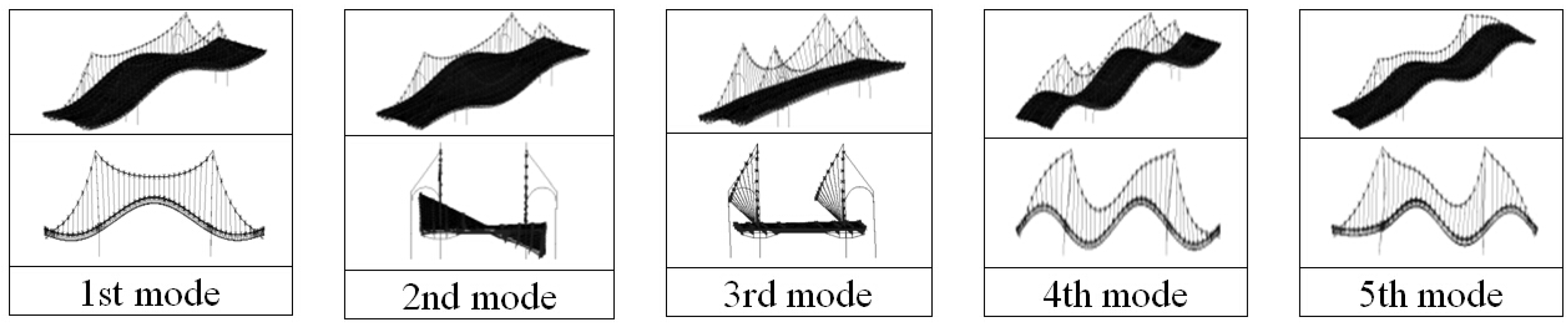
4.3. Analysis of Dynamic Characteristics

Both the theoretical and experimental analysis of dynamic characteristics of Hunan Road Bridge are conducted. The experiment mainly focused on the dynamic characteristic of main girder using ambient vibration test. From the FE model, the first five mode shapes of girders of Hunan Road Bridge are obtained and shown in Figure 5.

Table 3. Detail dynamic characteristics of main girder from theoretical and experimental analysis ¹.

Mode	Theoretical Frequency/Hz	Modal Shape	Experimental Frequency/Hz	Difference/%	MAC 2
1	0.7208	First order of vertical bending	0.9030	25.28	0.979
2	1.0643	First order of torsion	1.3670	28.44	0.973
3	1.3378	First order of transverse bending	1.3790	3.08	0.915
4	1.3892	Second order of vertical bending	1.9290	38.60	0.894
5	1.7504	Third order of vertical bending	2.4170	38.08	0.849

¹ $\mathrm{Difference}=\frac{|\mathrm{Experimental}\mathrm{Frequency}-\mathrm{Theoretical}\mathrm{Frequency}|}{\mathrm{Theoretical}\mathrm{Frequency}}\times 100\%$; ² MAC, Model assurance criteria.

shows dynamic characteristics of main girder from theoretical analysis and experimental data. Furthermore, the values of MAC (Model assurance criteria) are shown in Table 3. Based on test data, the damping ration of mode shape No. 1 and No. 4 in Table 3 are 2.40% and 1.59%, respectively. Thus, in Rayleigh ratio, the coefficients of alpha and beta are set as 0.038 and 0.006, respectively.

From the results of the main girder in Table 3, except the difference between theoretical and experimental frequencies of first order, transverse bending mode is 3.08%. Other differences are all above 25% in which the difference of second order of vertical bending frequency is even up to 38.6%. However, the MACs show that the experimental vibration modes have a relatively high agreement with the simulated ones, all of the MACs are over 0.84. This phenomenon indicates that a big difference exists in mode frequencies between the real bridge and the FE model which must be updated to reflect the real dynamic performance. Moreover, due to the extra-width, the torsion mode emerges earlier than ordinary bridges, which enhances the importance of yielding a precise FE model for further performance evaluation.

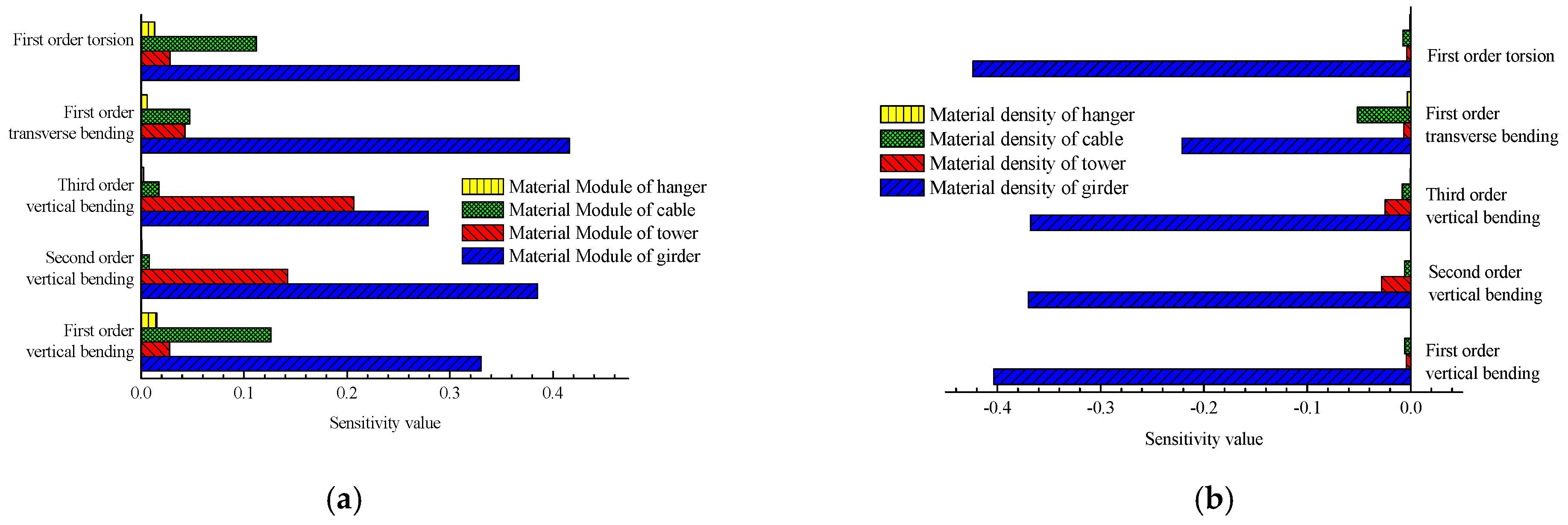
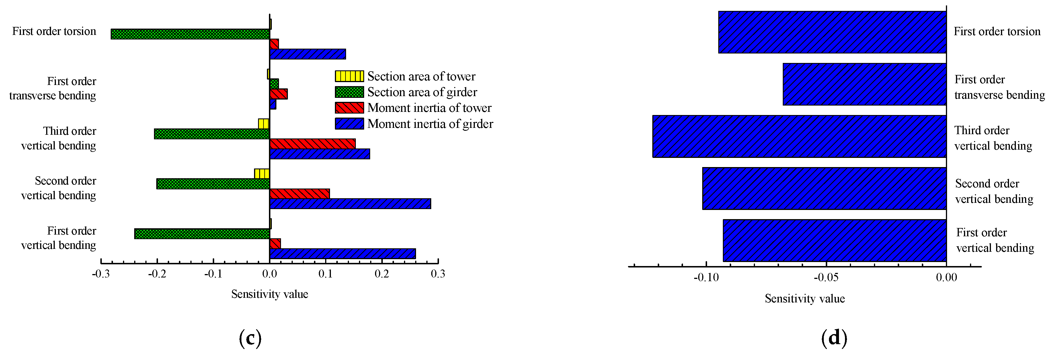
4.4. Parameters Selected by Sensitivity Analysis

Before analysis of model updating, the sensitivity of parameters, material modules (shown in Figure 6a), material densities (shown in Figure 6b), section characteristics (shown in Figure 6c), and secondary dead load (shown in Figure 6d), to frequencies like first, second, and third order vertical bending, first order transverse bending, and first order torsion are all taken into consideration. Parameters with a sensitivity value beyond ±0.1 are considered to be sensitive ones in this paper in which the value is computed by following formula,

$$\frac{\partial {\mathsf{\lambda }}_j(a_i)}{\partial a_i}=\frac{{\mathsf{\delta }\mathsf{\lambda }}_j}{{\mathsf{\lambda }}_j}/\frac{\mathsf{\delta }{a}_i}{a_i}$$

(12)

where $\mathsf{\delta }{\mathsf{\lambda }}_j$ is a small perturbation of the jth modal frequency of ${\mathsf{\lambda }}_j$, $\mathsf{\delta }{a}_i$ is a small perturbation of the ith parameter of $a_i$. Negative value of sensitivity value indicates negative influence when parameters increase.

In Figure 6a, the material module of girder is sensitive to first three order vertical bending, transverse bending, and torsion with value of 0.33, 0.39, 0.28, 0.42, and 0.37 respectively; the material module of tower is sensitive to second and third order vertical bending with value of 0.14 and 0.21; the material module of cable is sensitive to first order vertical bending and torsion with values of 0.13 and 0.11 while the material module of hanger shows no sensitivity to frequencies as all values are below 0.02. In Figure 6b, the material density of girder is sensitive to first three order vertical bending, transverse bending, and torsion with value of −0.40, −0.37, −0.37, −0.22, and −0.42 respectively while the other material densities show no sensitivity. In Figure 6c, the moment inertia of girder shows sensitivity to first three order vertical bending and torsion with value of 0.26, 0.29, 0.18, and 0.14 respectively when the moment inertia of tower just shows sensitivity to second and third order vertical bending with value of 0.11 and 0.16; just the section area of girder shows the same sensitivity of moment inertia of girder to frequencies with value of −0.24, −0.20, −0.21, and −0.28, while the area of the tower shows no sensitivity. In Figure 6d, the secondary dead load shows a little sensitivity to all frequencies as all values are around −0.1. To research more details, the moment of inertia of girder is divided into three parameters, namely moment inertia of vertical bending, transverse bending, and torsion. The whole results indicate that the selected sensitive parameters are material module of main girder, main tower and main cable, density of main girder, moment of inertia of vertical bending, transverse bending and torsion, moment of inertia of main tower, area of section of main girder, and secondary dead load, respectively.

4.5. Model Updating Using Proposed Hybrid Method

In the hybrid method, a particle is described as $X_i=[x_{i1},x_{i2},\cdot \cdot \cdot ,x_{i10}]$ with 10 parameters aforementioned of the ratio coefficients (real value/original value). For example, the parameter vector of initial FE model is [1,1,1,1,1,1,1,1,1,1]. The lower and upper boundary of each parameter is 0.5 and 1.5, and 400 input samples are yielded with the LHS technique. After the structural analyses, the output datasets of the aforementioned five natural mode frequencies are achieved. Then based on the input and output datasets, the Kriging meta-models of those five frequencies can be yielded. Finally, the objective function is the sum of residuals of mode frequencies of the first five modes between explicit expression value and experimental value. For GMPSO, the amount of particles N is 200, the inertia weight w is 0.55, the positive learning coefficients c₁ and c₂ are both 2, the probability of P_m is set as 0.1 and the maximum iteration number is 200, the optimized boundary is 0.6 to 1.4. The final updated parameters of the model of the self-anchored suspension bridge are [1.394,1.324,1.100,1.166,1.281,1.262,1.038,1.240,0.703,0.803].

The mode frequencies results of updated model and experimental data are compared in

Table 4. The comparison between modified and real frequencies.

Mode	Experimental Frequency/Hz	Updated Frequency/Hz	Difference/%
1	0.9030	0.9161	1.45
2	1.3670	1.3427	1.78
3	1.3790	1.4600	5.87
4	1.9290	1.8246	5.41
5	2.4170	2.2810	5.63

¹ $\mathrm{Difference}=\frac{|\mathrm{Updated}\mathrm{Frequency}-\mathrm{Experimental}\mathrm{Frequency}|}{\mathrm{Experimental}\mathrm{Frequency}}\times 100\%$.

. Figure 7 shows the comparison of vibration mode among initial FE value, updated value, and experimental value. The right column of Figure 7 is the 3-D image of mode shapes from ambient vibration test. It can be seen that the differences of frequencies in Table 3 dropped sharply in Table 4, all of the differences are below 6%. In addition, the values of MAC of vibration mode of No. 1 to No. 5 between test and initial FE model are 0.979, 0.973, 0.915, 0.894, and 0.849 respectively in Figure 7 while the MACs between test and modified FE model are 0.983, 0.974, 0.916, 0.873, and 0.882, respectively. This shows that the vibration modes of the updated bridge model have a higher agreement with the experimental value shown in Figure 7, although the increases in MACs are insignificant compared to that in mode frequencies. The whole changes indicate that the relatively precise FE model of this self-anchored suspension bridge with extra-width can be achieved with high efficiency without losing accuracy and the proposed hybrid method does have significant value in model updating of engineering applications.

5. Conclusions

In this article, a hybrid model updating method by integration of GMPSO and Kriging meta-model has been proposed. Compared to ordinary polynomial meta-models, the stochastic process in Kriging meta-model increases the accuracy, and meanwhile, it first uses the LHS technique to improve the quality of input datasets. Compared to direct GMPSO method, the only FE analysis calls are used in forming the Kriging meta-model. By combining advantages of both GMPSO and Kriging meta-model, the proposed hybrid method can prohibitively reduce the computation time without losing accuracy. Thus, this method is suitable for model updating of engineering applications with large-scale, multi-dimensional parameter structures involving implicit performance functions. After the validation study of this hybrid method and its application to a self-anchored suspension bridge with extra-width located in China, several conclusions can be drawn from this article as follows:

• Through the application of the hybrid method to a damaged simply supported beam, it was evident that the updating process of hybrid method, compared to direct GMPSO, can be performed more efficiently without losing accuracy. This demonstrates that the proposed hybrid method is applicable to model updating of engineering applications.
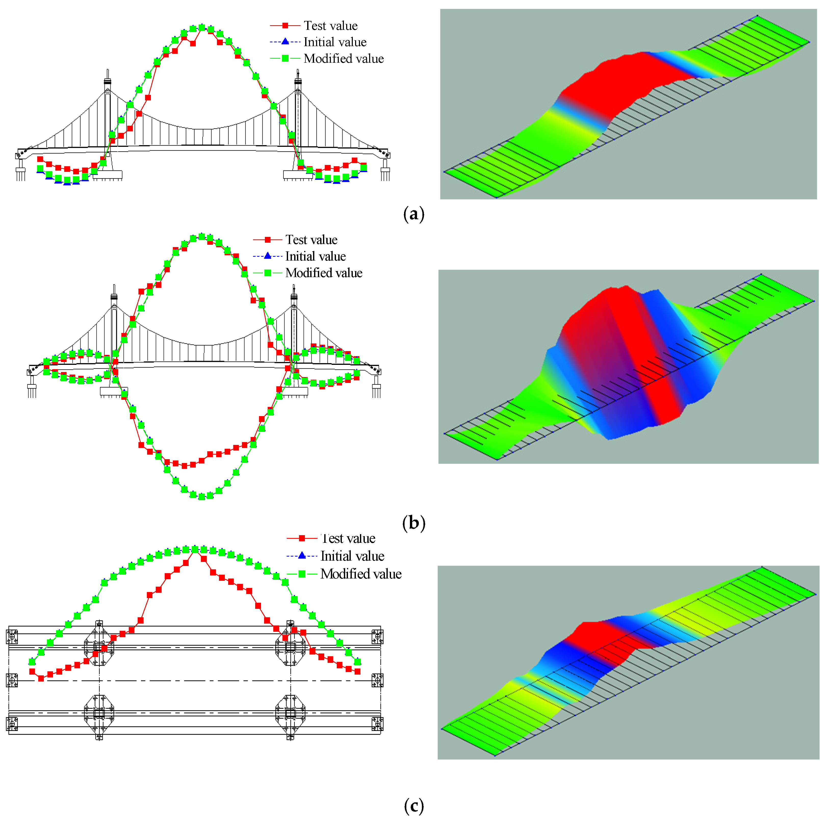
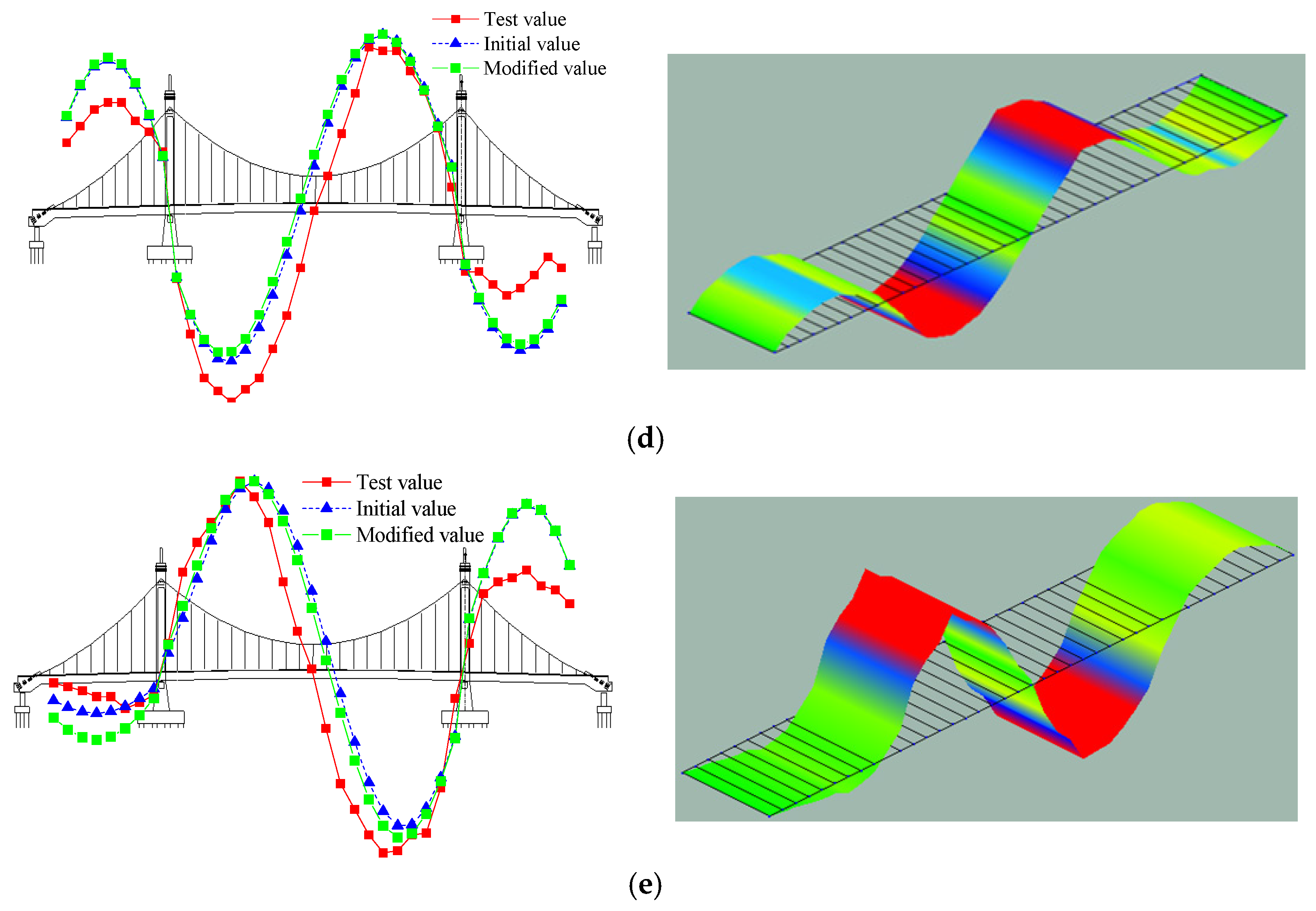
• Based on the mode frequency results of ambient vibration test of Hunan Road Bridge, it was clear seen that the differences between the initial FE model and experiment were large enough, some of which are up to 38%, but the vibration modes show high agreements with a lowest MAC value of 0.849. Moreover, due to the extra-width, the torsion mode emerged earlier than ordinary bridges, which enhanced the importance of yielding a precise FE model for further performance evaluation.
• Ten sensitive parameters—module of main girder, main tower and main cable, density of main girder, moment of inertia of vertical bending, transverse bending and torsion, moment of inertia of main tower, area of section of main girder, and secondary dead load—were selected after sensitivity analysis as updated parameters of Hunan Road Bridge. After model updating using hybrid method, both of the mode frequencies and shapes showed a relatively high agreement with the results of the experiment. The differences of mode frequencies drop sharply and are all below 6%. Meanwhile, all the MACs increase over 0.87, which indicates the vibration mode has a higher agreement. The successful model updating of this bridge fills in the blank of model updating of a complex self-anchored suspension bridge. In addition, the updating process makes it possible for other model updating issues of complex bridge structures.

References

1. Li, J.; Li, A.; Feng, M. Sensitivity and reliability analysis of a self-anchored suspension bridge. J. Bridge Eng. 2013, 18, 703–711. [Google Scholar] [CrossRef]
2. Kaloop, M.R.; Hu, J.W.; Elbeltagi, E. Evaluation of high-speed railway bridges based on a nondestructive monitoring system. Appl. Sci. 2016, 6, 24. [Google Scholar] [CrossRef]
3. Kim, S.H.; Won, J.H. Structural behavior of a long-span partially earth-anchored cable-stayed bridge during installation of a key segment by thermal prestressing. Appl. Sci. 2016, 6, 231. [Google Scholar] [CrossRef]
4. Feng, D.; Scarangello, T.; Feng, M.; Ye, Q. Cable tension force estimate using novel noncontact vision-based sensor. Measurement 2017, 99, 44–52. [Google Scholar] [CrossRef]
5. Zhao, H.W.; Ding, Y.L.; An, Y.H.; Li, A.Q. Transverse dynamic mechanical behavior of hangers in the rigid tied arch bridge under train loads. J. Perform. Constr. Facil. 2017, 31, 04016072. [Google Scholar] [CrossRef]
6. Wang, G.X.; Ding, Y.L.; Song, Y.S.; Wu, L.Y.; Yue, Q.; Mao, G.H. Detection and location of the degraded bearings based on monitoring the longitudinal expansion performance of the main girder of the Dashengguan Yangtze Bridge. J. Perform. Constr. Facil. 2016, 30, 04015074. [Google Scholar] [CrossRef]
7. Liu, Z.; Guo, T.; Chai, S. Probabilistic fatigue life prediction of bridge cables based on multiscaling and mesoscopic fracture mechanics. Appl. Sci. 2016, 6, 99. [Google Scholar] [CrossRef]
8. Ding, Y.; Li, A. Finite element model updating for the Runyang cable-stayed bridge tower using ambient vibration test results. Adv. Struct. Eng. 2008, 11, 323–335. [Google Scholar] [CrossRef]
9. Guo, J.; Zhong, J.; Dang, X.; Yuan, W. Seismic responses of a cable-stayed bridge with consideration of uniform temperature load. Appl. Sci. 2016, 6, 408. [Google Scholar] [CrossRef]
10. Cismaşiu, C.; Narciso, A.; Amarante dos Santos, F. Experimental dynamic characterization and finite-element updating of a footbridge structure. J. Perform. Constr. Facil. 2014, 29, 04014116. [Google Scholar] [CrossRef]
11. Deng, L.; Cai, C.S. Bridge model updating using response surface method and genetic algorithm. J. Bridge Eng. 2010, 15, 553–564. [Google Scholar] [CrossRef]
12. Berman, A.; Flannelly, W.G. Theory of incomplete models of dynamic structure. AIAA J. 1970, 9, 1481–1487. [Google Scholar] [CrossRef]
13. Chen, J.C.; Graba, J.A. Analytical model improvement using modal test results. AIAA J. 1980, 18, 684–690. [Google Scholar] [CrossRef]
14. Wan, H.; Ren, W. Parameter selection in finite-element-model updating by global sensitivity analysis using Gaussian process metamodel. J. Struct. Eng. 2014, 141, 04014164. [Google Scholar] [CrossRef]
15. Feng, D.; Feng, M. Model updating of railway bridge using in situ dynamic displacement measurement under trainloads. J. Bridge Eng. 2015, 20, 04015019. [Google Scholar] [CrossRef]
16. Perera, R.; Torres, R. Structural damage detection via model data with genetic algorithms. J. Struct. Eng. 2006, 132, 1491–1501. [Google Scholar] [CrossRef]
17. Marwala, T. Finite element model updating using response surface method. In Proceedings of the 45th Collection of Technical Papers-AIAA/ASME/ASCE/AHS/ASC Structures, Structural Dynamics and Materials Conference, Palm Springs, CA, USA, 19–22 April 2004; pp. 5165–5173.
18. Gholizadeh, S.; Moghadas, R.K. Performance-based optimum design of steel frames by an improved quantum particle swarm optimization. Adv. Struct. Eng. 2014, 17, 143–156. [Google Scholar] [CrossRef]
19. Xiang, J.; Zhong, Y. A novel personalized diagnosis methodology using numerical simulation and an intelligent method to detect faults in a shaft. Appl. Sci. 2016, 6, 414. [Google Scholar] [CrossRef]
20. Si, L.; Wang, Z.; Liu, Z.; Liu, X.; Tan, C.; Xu, R. Health condition evaluation for a shearer through the integration of a fuzzy neural network and improved particle swarm optimization algorithm. Appl. Sci. 2016, 6, 171. [Google Scholar] [CrossRef]
21. Nanda, B.; Maity, D.; Maiti, D.K. Crack assessment in frame structures using modal data and unified particle swarm optimization technique. Adv. Struct. Eng. 2014, 17, 747–766. [Google Scholar] [CrossRef]
22. Kaveh, A.; Nasrolahi, A. A new probabilistic particle swarm optimization algorithm for size optimization of spatial truss structures. Int. J. Civ. Eng. 2014, 12, 1–13. [Google Scholar]
23. Do, D.M.; Gao, W.; Song, C.; Tangaramvong, S. Dynamic analysis and reliability assessment of structures with uncertain-but-bounded parameters under stochastic process excitations. Reliab. Eng. Syst. Saf. 2014, 132, 46–59. [Google Scholar] [CrossRef]
24. Liao, Z.X.; Zhong, W.M.; Qian, F. Particle swarm optimization algorithm based on mutation of Gaussian white noise disturbance. J. East China Univ. Sci. Tech. (Nat. Sci. Ed.) 2008, 34, 859–863. (In Chinese) [Google Scholar]
25. Ren, W.X.; Fang, S.E.; Deng, M.Y. Response surface-based finite-element-model updating using structural static responses. J. Eng. Mech. 2011, 137, 248–257. [Google Scholar] [CrossRef]
26. Simon, P.; Goldack, A.; Narasimhan, S. Mode shape expansion for lively pedestrian bridges through Kriging. J. Bridge Eng. 2016, 21, 04016015. [Google Scholar] [CrossRef]
27. Dette, H.; Pepelyshev, A. Generalized Latin hypercube design for computer experiments. Technometrics 2010, 52, 421–429. [Google Scholar] [CrossRef]
Figure 1. Gaussian mutation particle swarm optimization (GMPSO) algorithm flowchart.
Applsci 07 00191 g001
Figure 2. Flowchart of proposed hybrid method for model updating.
Applsci 07 00191 g002
Figure 3. A 10 m-span beam structure (unit: cm).
Applsci 07 00191 g003
Figure 4. Description of Hunan Road Bridge: (a) Image of Hunan Road Bridge; (b) Image of Hunan Road Bridge; (c) FE model of Hunan Road Bridge.
Applsci 07 00191 g004
Figure 5. The first five modal shapes of main girder of Hunan Road Bridge from FE model.
Applsci 07 00191 g005
Figure 6. Sensitivity of parameters to frequencies: (a) Sensitivity of material modules to frequencies; (b) Sensitivity of material densities to frequencies; (c) Sensitivity of section characteristics to frequencies; (d) Sensitivity of secondary dead load to frequencies.
Applsci 07 00191 g006aApplsci 07 00191 g006b
Figure 7. Comparisons of each vibration mode and images of each vibration mode form test: (a) Mode No. 1; (b) Mode No. 2; (c) Mode No. 3; (d) Mode No. 4; (e) Mode No. 5.
Applsci 07 00191 g007aApplsci 07 00191 g007b