Measurement and Modeling of a Cargo Bicycle Tire for Vehicle Dynamics Simulation

Featured Application

The presented Magic Formula model of a bicycle tire for cargo trailers can be used for the mathematical modeling and simulation of a bicycle trailer or vehicle without camber angle. Further, the model can be used in linearized or original form for the implementation of a vehicle dynamics controller on an ECU to consider the tire behavior.

Abstract

In the field of inner-city cargo transportation, solutions such as electrified cargo trailers are increasingly being used. To provide an intelligent drivetrain control system that improves driving dynamics and enables safety, it is necessary to know the characteristics of the trailer system. This includes the behavior of the tires. Existing investigations of bicycle tires focus on camber-angle-dependent models. However, in most trailers, a rigid mounting of the tires without camber is used. For this reason, a bicycle tire model is created within the scope of this study using real measurement data that represent a 20 in tire with typical wheel loads and without camber. The measurements were collected with the mobile tire measurement laboratory of the Bern University of Applied Sciences on an asphalt test site under real conditions. Crosstalk occurring in the measurement hub during the data collection was successfully corrected using a matrix method. With help of the so-called Magic Formula, a tire model was created that can be used for driving dynamics simulations and controller design.

1. Introduction

The general demand for a supply chain that is sustainable up to the last mile requires new transportation systems. In urban areas, solutions such as cargo bicycles and trailers are becoming increasingly popular. These are stable bicycles and trailers that enable the transportation of large and heavy loads. To cope with this additional load, many small cargo transportation systems such as [1,2,3] are equipped with electric drives for support. However, even without electrification, the systems place high demands on the user’s driving skills, since, according to [4], hitching up a towing vehicle is a major modification of the system’s driving dynamics. In addition, inexperienced users have considerable difficulties predicting the self-dynamics of a loaded cargo trailer for a bicycle. If the system is equipped with an electric drive, the torque must be controlled in order to avoid dangerous driving situations. This also includes the phenomena of snaking and jack-knifing. While, according to [5], snaking results from lateral forces pushing the trailer from one side to the other, jack-knifing is due to tire–ground interactions. In this case, especially during heavy braking or driving through a curved road, the transmissible force of the tire on the road becomes saturated, which can be triggered by the additional mass of the trailer to be braked. If there is also an angle between the trailer and the towing vehicle so that their x-axes are not parallel-aligned, the angle can be increased by the sliding towing vehicle and the pushing trailer until the systems collide. In addition to the dependence on the loading position, ref. [6] underlines the central part of the tire behavior in the described phenomena. In this context, refs. [7,8] point out the importance of tire behavior. If measurements can be used to model the tire behavior, they can be taken into account in the design of a subsequent control system. To counteract snaking and jack-knifing of the system, refs. [9,10] show exemplary different control approaches, which are all based on known tire behavior and, thus, on a tire model. For the majority of cases, linearized tire models are used, which result from a factor repesenting tire stiffness and its dependence on the slip angle. Furthermore, according to the studies of [11,12], a major impact on the evaluation of a vehicle’s efficiency results from the tire behavior. In this context, measurement and modeling can also contribute to system optimization.

If the driving behavior of cargo trailers in the field of micromobility is to be investigated or a driving dynamics control of the electric drive is to be realized, the behavior of the tires in use must also be studied more closely. However, knowledge of the tire behavior of typical bicycle tires for this application purpose is lacking for the design and parameterization of intelligent control algorithms.

Existing studies, such as that of [13], cover the modeling of a wide range of bicycle tires, which are designed for conventional bicycle driving and not load transportation. Additional investigations carried out by [14] show the measurements of mountain bike tires on a test bench, as well as the generation of a mathematical magic formula model from the resulting data. The author points out that, due to the limitations of the test rig, a side-slip angle greater than +/−$2^{°}$ could not be investigated. In addition, the tires are measured at different camber angles, since, in the normal use of a bicycle, cornering is performed by turning and tilting the bicycle towards the inside of the corner. Reference [15] shows similar tests, where the focus is on the comparison of different road tires.

As part of this research work, a special tire for cargo bikes and trailers was measured on asphalt with the help of the mobile tire testing laboratory (MoReLab) at the Bern University of Applied Sciences (BFH). The focus of this work is not on comparing different tires, but on measuring one tire of a common size for cargo trailers under different conditions and creating a precise mathematical tire model based on the research of [16]. The novelty of the findings presented in this paper results from the measurement of a special tire for cargo bikes and trailers under specific boundary conditions, which include a camber angle of $0^{°}$ on a flat asphalt surface and a common vehicle velocity. In addition, the tire was measured on a mobile test truck, which was developed to measure truck and car tires. As a result, the present research confirms the use of the test truck in the field of micromobility applications. The findings and models created within the present work can significantly contribute to further research on the design of vehicle dynamics control or efficiency analysis for vehicles from the micromobility sector with the help of simulation. In conclusion, this work provides a deeper knowledge of bicycle tires for use in load transportation applications.

2. Materials and Methods

This section explains the test set-up that was used to measure the tire in more detail. Furthermore, the adjustable parameters of the tire are described, as well as the test matrix thatwas used for the examination. In addition, the mathematical modeling of tires used in this research work and developed by [16] is explained.

2.1. Measurements

2.1.1. Mobile Tire Testing Laboratory

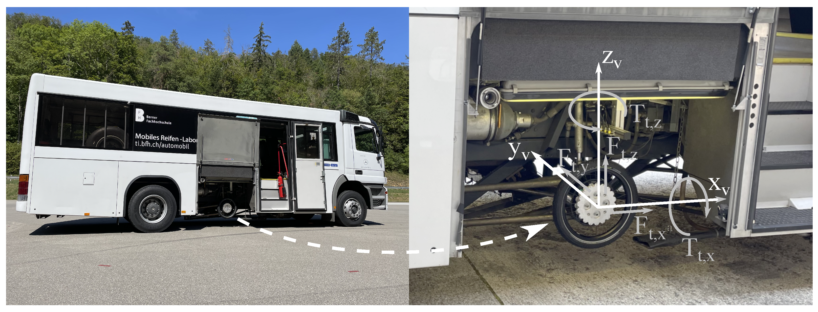
The MoReLab, which can be seen in Figure 1, is a truck with two possible test wheels that can be mounted in the middle between the front and rear axles on each side. A special measurement hub with load cells was used to record longitudinal and lateral forces, as well as torques acting from the tire towards the hub. The signals from the measurement hub were sampled and recorded at a frequency of 250 Hz and contain:

• Longitudinal tire force $F_{t,x}$;
• Lateral tire force $F_{t,y}$;
• Vertical tire force $F_{t,z}$;
• Torque around x-axis $T_{t,x}$;
• Torque around z-axis, also referred to as aligning torque $T_{t,z}$.

The test wheel was propelled by a hydraulic drive, which enables the wheel to be operated even at high slip values. Because of this, even unstable slip ranges can be measured accurately. Since the drive shaft does not have an external brake, the torque $T_{t,y}$ could not be measured with this setup.

Because the truck can move on almost any surface, real test tracks can be driven with the vehicle. Compared to the indoor test benches listed in [13,14,15], this leads to some advantages and disadvantages. Measurements can be taken on surfaces ranging from asphalt to very coarse gravel, while gravel in particular cannot be optimally reproduced in indoor systems. However, indoor test facilities create comparable initial conditions, while the tests with the MoReLab are carried out outdoors under changing but real environmental conditions. Possible measurements that can be carried out with the presented system are listed below:

• Spinning the test wheel faster than the truck’s constant speed $v_{v,x}$ and recording $F_{t,x}$ respective to the longitudinal slip $\kappa$ (driving);
• Spinning the test wheel slower than the truck’s constant speed $v_{v,x}$ and recording $F_{t,x}$ respective to the longitudinal slip $\kappa$ (braking);
• Steering the freewheeling test wheel with a slip angle $\alpha$ from $-2^{°}$ to ${18}^{°}$ with the truck driving in a straight line to record the Force $F_{t,y}$ and aligning torque $T_{t,z}$ (steering);
• Combined measurements of spinning the wheel faster or slower than the truck’s constant speed $v_{v,x}$ while a slip angle $\alpha$ from $-2^{°}$ to ${18}^{°}$ is applied and the truck is driving in a straight line to record the Force $F_{t,y}$ and aligning torque $T_{t,z}$ (steering with combined slip—not covered in this research).

To capture the recorded forces in relation to the slip $\kappa$, Equations (1) and (2) were used to calculate the slip according to the data measured by the system.

Drive slip:

$${\kappa }_d=\frac{v_{t,x}-v_{v,x}}{v_{t,x}}·100\%$$

(1)

Brake slip:

$${\kappa }_b=\frac{v_{v,x}-v_{t,x}}{v_{v,x}}·100\%$$

(2)

For this purpose, the measurement system of the test truck provides the measured wheel speed $v_{t,x}$ of the test wheel to the user, which is calculated with the aid of Equation (3). $r_e$ is defined as the measured effective rolling radius of the tire at the examined speed and $\omega$ is the wheel speed measured by hall sensors.

$$v_{t,x}=r_e·\omega$$

(3)

The actual longitudinal speed of the test truck $v_{v,x}$ was recorded with the aid of a laser surface measurement. To relate $F_{t,y}$ and $T_{t,z}$ with respect to the slip angle $\alpha$, the system can measure this angle directly during measurement using an analog angle sensor, which is mechanically connected to the measurement hub. It must be noted that the mechanical design of the test truck does not allow for $\alpha$ values smaller than −$2^{°}$, as otherwise the wheel mount and test wheel may collide. This also applies to the positive range of $\alpha$, where the wheel can be turned up to ${18}^{°}$ degrees. A range of −$2^{°}$ to ${18}^{°}$ was thus obtained for $\alpha$. Furthermore, the system offers various variable parameters that can be set by the operator for different experiments with the test truck. These include:

• Normal Force $F_{N,z}$, which depends on the mass distribution of the vehicle. $F_{N,z}$ results from the average value of $F_{t,z}$ in $F_{N,z}={\overline{F}}_{t,z}$.;
• Longitudinal speed $v_{v,x}$ at which the measurements are to be carried out;
• Slip angle $\alpha$;
• Camber angle $\gamma$.

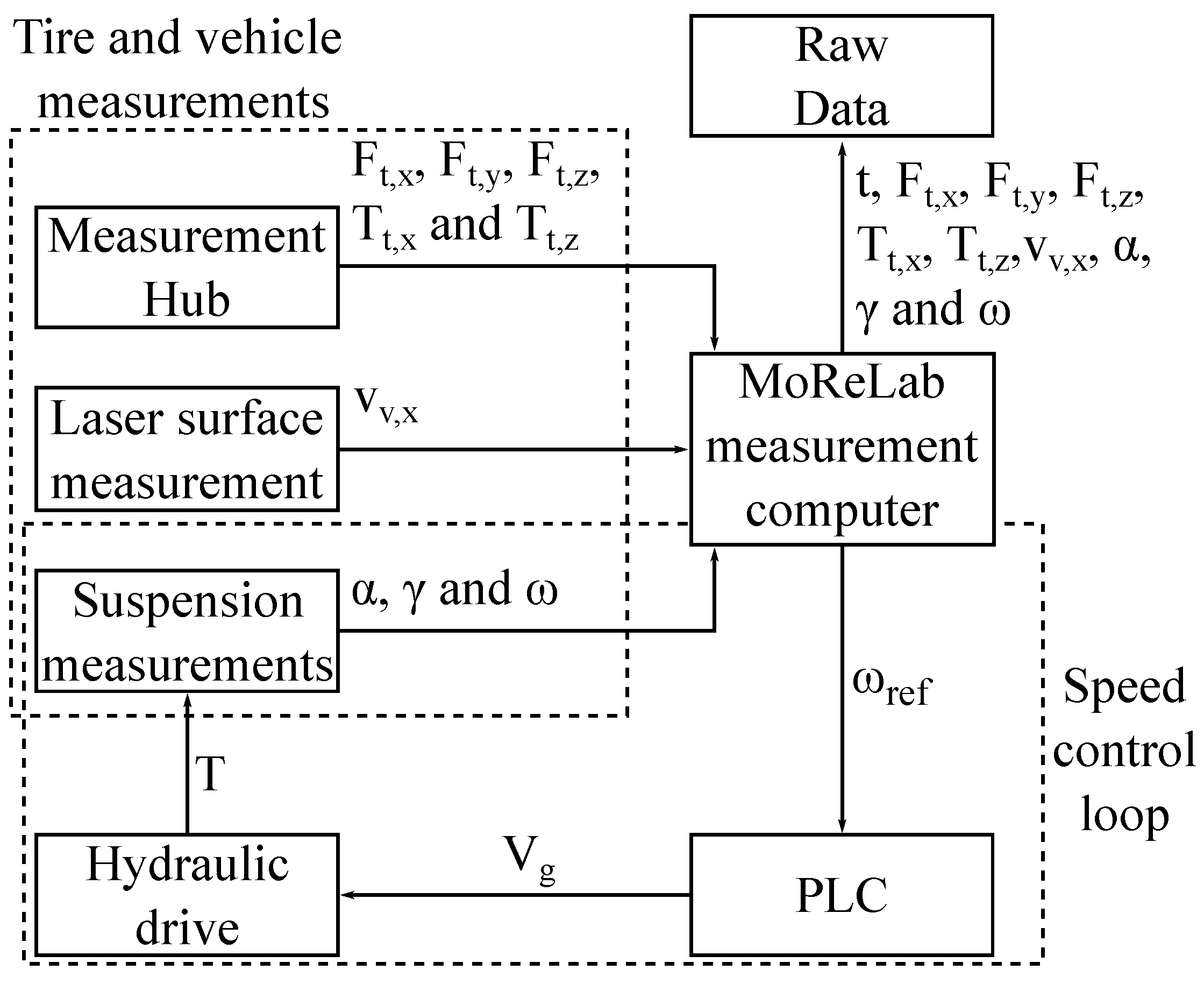
An overview of the measurement system up to the raw data output is shown graphically for the test truck in Figure 2. The measured variables described above are collected via the sensors, sampled by the central computer in the test truck, and provided with a time stamp t. The merged data are stored and can be saved as raw data after the completion of a test. The recorded raw data serve as a starting point for the upcoming post-processing.

For a better understanding, Figure 2 also shows the speed control loop of the hydraulic drive. Here, the target wheel speed ${\omega }_{ref}$ required by the user, depending on the case, is transmitted from the central computer to the PLC. The PLC then calculates the displacement volume $V_g$, which serves as the control variable for the hydraulic drive. This results in a wheel torque T, which acts on the system and, in turn, influences the actual wheel speed $\omega$. The control loop is completed by measuring $\omega$ using a wheel speed sensor and transmitting this to the central computer of the test truck.

As the MoReLab was developed for the automotive sector, measurement rims from a diameter of 13 in (330.2 mm) upwards with an offset of 60 mm is used as standard. The diameter of 13 in (330.2 mm) results from the size of the measurement hub, which would interfere with the measurement rim at smaller diameters. The offset 60 mm ensures that the center contact point of the tire $P_p$ is in line with the center of the measurement hub. This prevents the development of unintended torques from resulting lever arms and therefore reduces the occurrence of crosstalk.

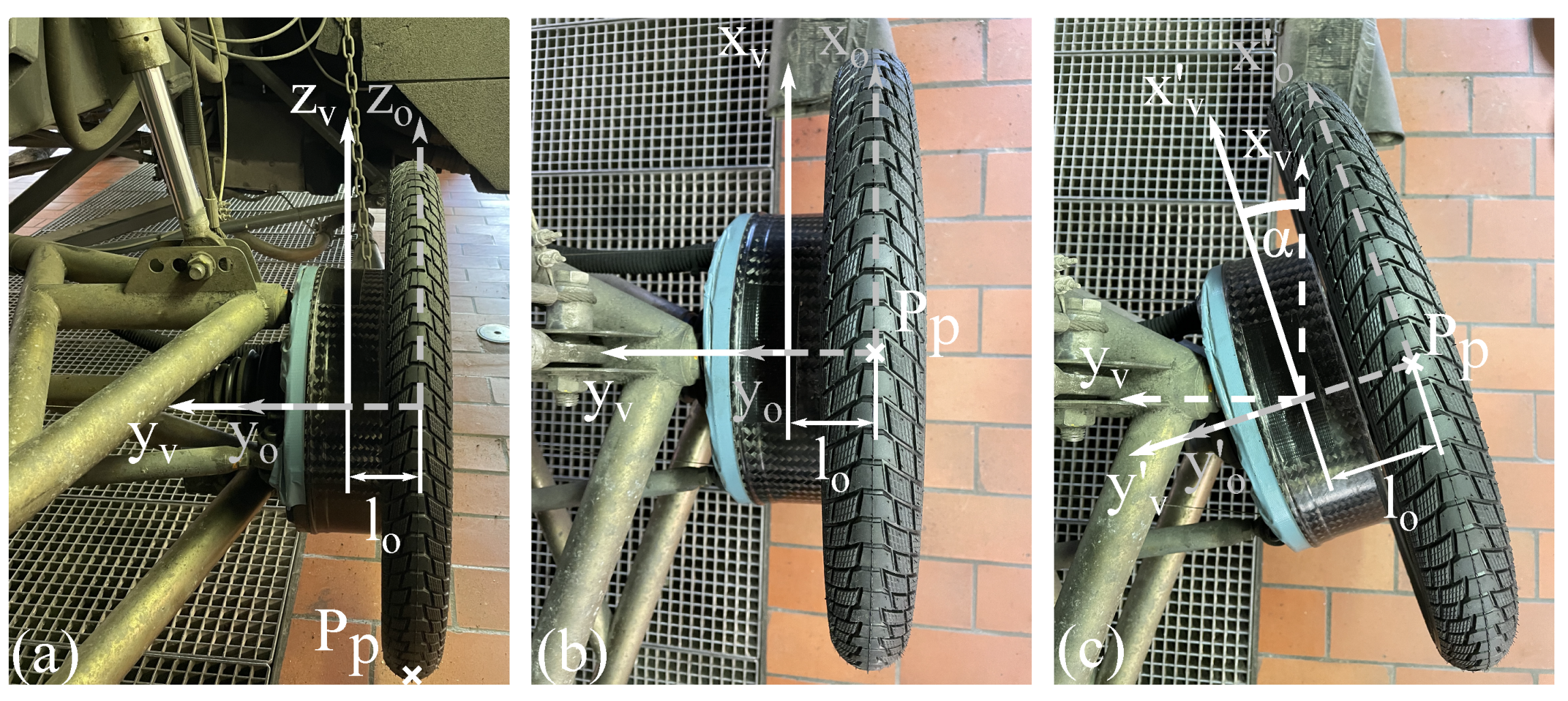
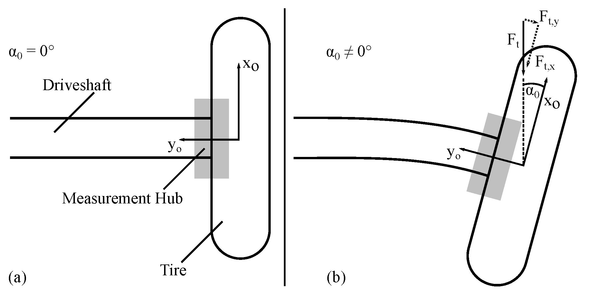
Due to the research of [13], which claims that the measurement of bicycle tires should be as realistic as possible compared with the real use-case, a special adapter rim for 20 in (508 mm) wheels with spokes was used. The spoke length of the adapter rim was the same as the spoke length of the wheel-motor combination often used in electrified trailers and equals 75 mm. However, the diameter of the adapter rim was almost the same as the diameter of the measurement hub, which only allows for an offset of 5 mm to be realized. This leads to the disadvantage that the contact point of the tire $P_p$ was no longer in the center of the measurement hub, but shifted towards the positive $y_v$ direction of the vehicle. The displacement of the tire’s coordinate system ($x_o$, $y_o$ and $z_o$) and the measurement hub’s coordinate system ($x_v$, $y_v$ and $z_v$) due to the respective adapter rim, as well as the resulting lever arm $l_o$, are shown in Figure 3.

Due to the lever arm $l_o$, torques about the $z_v-$ and $x_v-$ axis arise for the case $\alpha =0^{°}$ and for $\alpha \ne 0^{°}$ while driving the test truck with the tire interacting with the ground during experiments, which, in addition, leads to crosstalk in the force channels of the measurement hub. For example, if an external force is applied only in $x_o$ direction, the resulting measurements will show nonzero values on all other channels. The same applies to the remaining directions in three-dimensional space. Therefore, crosstalk must be corrected by the user. Additionally, an offset compensation must be carried out. If the data have a large amount of scatter, smoothing or averaging can be used to reduce this effect.

Post-processing of the data is, therefore, divided into the following steps:

• Offset correction;
• x-, y- and z-axis crosstalk correction;
• If needed, smoothing the data.

2.1.2. Tire Parameters and Test Matrix

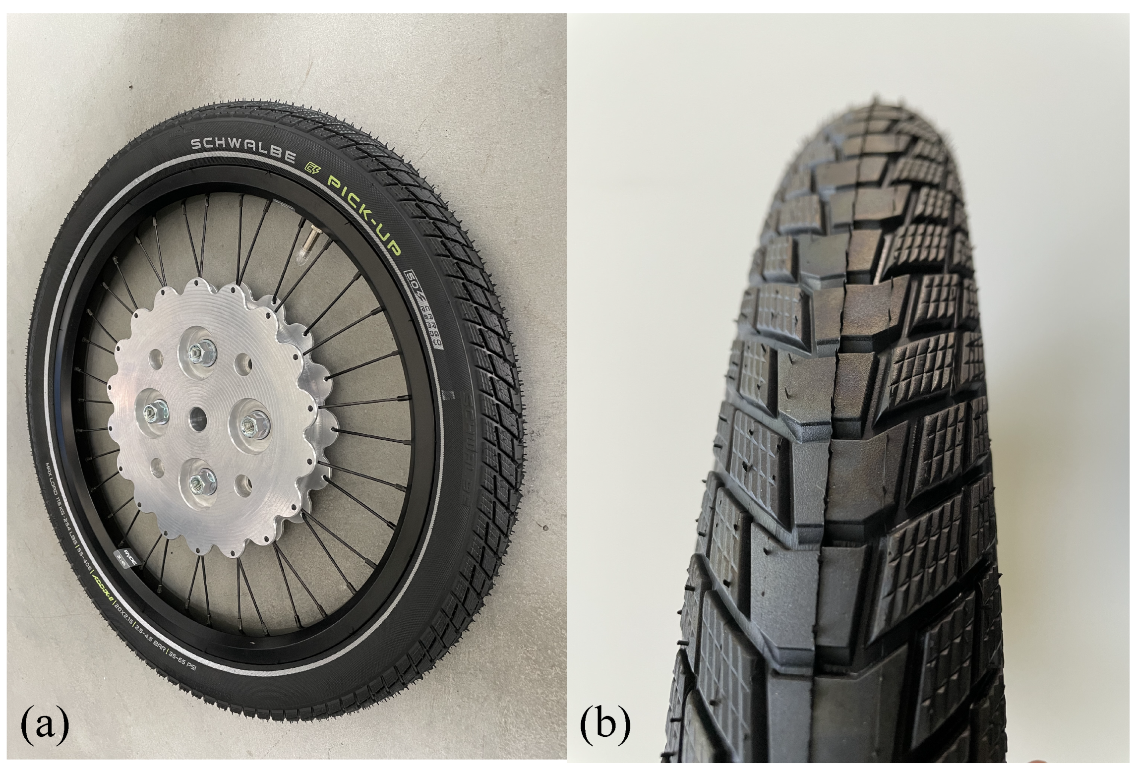
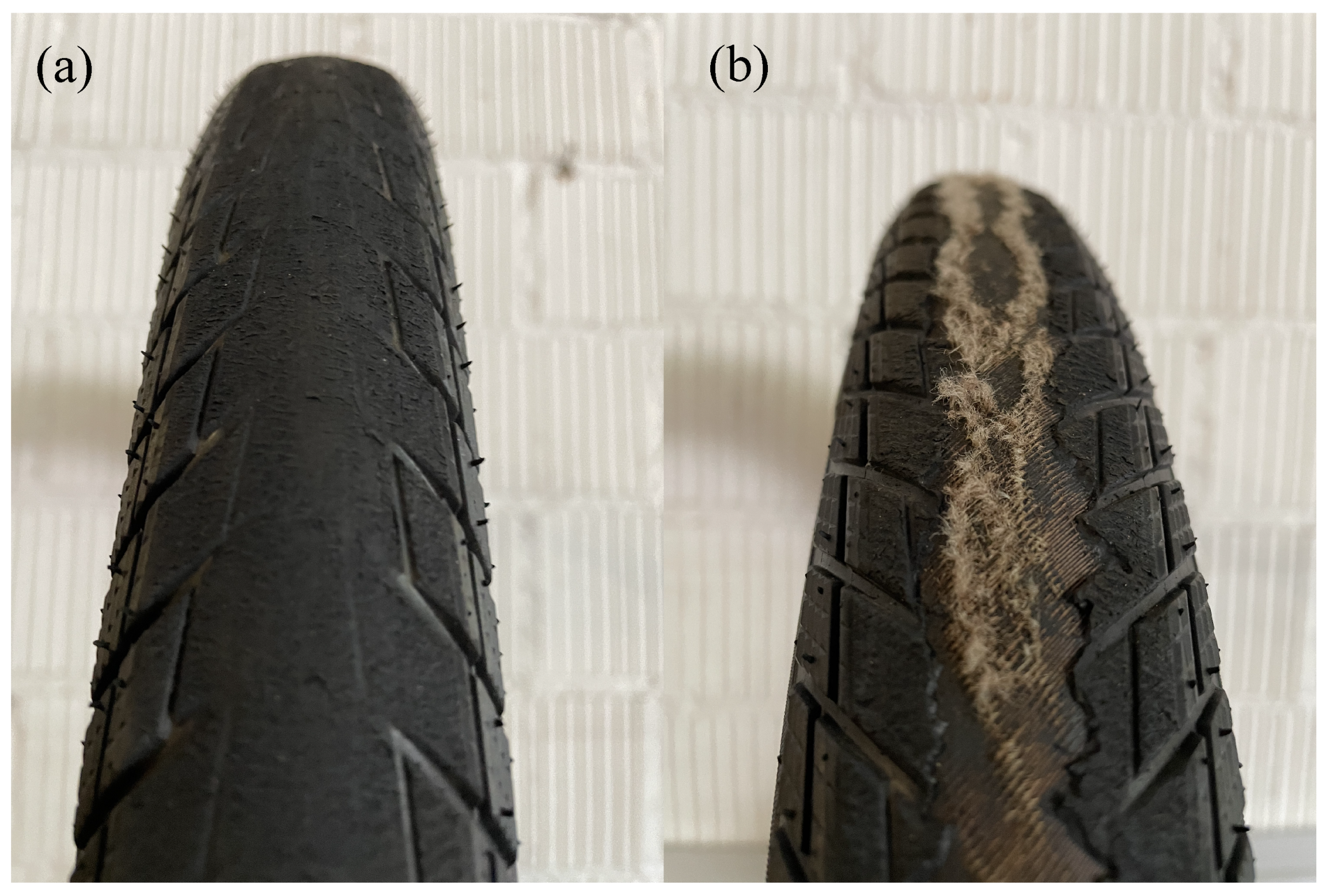
The chosen tire model is called “Pick-Up”, from the company Ralf Bohle GmbH, distributed by the brand name Schwalbe^®, which was specially developed for use in cargo bikes or trailers. The tested size of 55–406 ETRO (20 × 2.15 in) is a common tire choice for these applications. According to [17], this tire can be inflated with an air pressure of 2.5–4.5 bar (35–65 psi) and should mainly be used on asphalt or light gravel roads. In addition, the tire has a double wire carcass and puncture protection. The weight is listed as 0.790 kg. The tire mounted with an inner tube on the adapter rim is shown in Figure 4a. A view of the profile before tests were carried out can be seen in Figure 4b.

While many external influences impac the tire, the air pressure is an essential parameter that can be adjusted directly on the tire, on the valve of the inner tube. In combination with the setting options of the test truck, this results in numerous variable parameters, which are listed in

Table 1. Test matrix covered in this research.

Test No.	Tire Pressure p in psi	Tire Pressure p in bar	${\mathit{F}}_{\mathit{N},\mathit{z}}$ in N	${\mathit{v}}_{\mathit{v},\mathit{x}}$ in m/s	Range $\mathit{\alpha }$ in ${}^{°}$	$\mathit{\gamma }$ in ${}^{°}$
1.1	43.511	3.0	625	5.556	−2–18	0
1.2	43.511	3.0	765	5.556	−2–18	0
2.1	50.763	3.5	625	5.556	−2–18	0
2.2	50.763	3.5	765	5.556	−2–18	0
3.1	58.015	4.0	625	5.556	−2–18	0
3.2	58.015	4.0	765	5.556	−2–18	0

. To investigate the effects of tire pressure on the forces that can be transmitted, the pressure was selected within the range permitted by the manufacturer. The investifated tire pressures were 3.0, 3.5 and 4.0 bar. Since cargo trailers are intended for the transportation of heavy loads, the measurement of the tires was planned with a lower normal force of 500 N and an upper normal force of 750 N. However, the measurement equipment does not allow for fine adjustment, so the closest possible range of approx. 625 N as the lower and 765 N as the upper normal force was applied during the tests. Assuming an acceleration due to gravity of 9.81 $\frac{m}{s^2}$, this corresponds to a load of around 127 or 156 kg optimally distributed at the center of gravity for a trailer with one axle and two wheels. As cargo trailers are mainly operated with electrically assisted bicycles with an assistance of up to 25 km/h, the working range was assumed to be 20 km/h or 5.56 m/s, respectively. Therefore, the investigations were carried out at a constant speed of $v_{v,x}$ = 5.56 m/s of the test truck. Furthermore, the slip angle $\alpha$, which can be adjusted by the system from −2${}^{°}$ to 18${}^{°}$, was completely utilized. Since the present work essentially focuses on the investigation of bicycle tires for cargo trailers, which do not offer a camber angle or the possibility of tilting the tire into the curve, all investigations were carried out with a camber angle $\gamma$ of 0${}^{°}$. In this context, it must be noted that the measurements and the model derived from them are only representative for $\gamma =0^{°}$ on an even road surface. On uneven road surfaces, the vertical line of the contact patch is not in line with the tire centerline in the yz-plane, resulting in $\gamma \ne 0^{°}$. As the field of application for load trailers is mainly in urban areas, this case was not considered a priority in the present investigations.

As a result, Table 1 shows a total of six parameter combinations for measuring the tires. For each of the six combinations $F_{t,x}\left(\kappa \right)$, $F_{t,y}\left(\alpha \right)$ and $T_{t,z}\left(\alpha \right)$ are captured. Since $F_{t,x}\left(\kappa \right)$ has to be measured for driving and braking while $F_{t,y}\left(\alpha \right)$ and $T_{t,z}\left(\alpha \right)$ can be measured in the same steering case, the six parameter combinations of Table 1 must be multiplied with the three test cases (drive, brake, and steer) to obtain a total number of 18 test cases. From the experience of previous studies, each of the 18 test cases were found to require between 15 and 25 measurements to record an average representation of the behavior. In this context, it should be noted that several measurements can be carried out one after the other during a drive with the test truck as a measurement series, whereby the relaxation phase of the tire, as well as the wear, must be taken into account. In order to investigate $F_{t,x}\left(\kappa \right)$ for both the acceleration and braking cases, the PLC control of the measurement system must be used. During this process, the longitudinal velocity of the truck is kept constant at 5.556 m/s, while the hydraulic drive of the measurement system brakes or accelerates the test wheel. In the “Accelerate” case, the measurement wheel is first brought to a speed of 4.722 m/s and then accelerated to 11.111 m/s to ensure a proper zero transition. In the “Braking” case, the measurement wheel is initially moved at a velocity of 11.111 m/s. By decelerating to the speed of the truck, a braking process with 5.556 m/s is thus realized. During acceleration or braking to the final speed, the forces in the x-, y- and z-directions and the torque around the x- and z-axes are recorded. Furthermore, $F_{t,y}\left(\alpha \right)$ and $T_{t,z}\left(\alpha \right)$ are measured for a slip angle $\alpha$ of −2–18${}^{°}$, as large negative slip angles cannot be measured with the system due to mechanical restrictions. However, because of the symmetrical structure of bicycle tires, it is assumed that the absolute values of $F_{t,y}$ and $T_{t,z}$ are approximately the same for positive and negative slip angles. In addition, when measuring $F_{t,y}\left(\alpha \right)$ and $T_{t,z}\left(\alpha \right)$, no drive or braking torque is transmitted via the drive shaft of the measurement system, so the tire can roll free. Since the test truck was not designed for measuring vehicle tires in the micromobility class, many variables, such as $F_{N,z}$, cannot be set finely enough. As a result, overshoots are expected during the investigation of transient conditions, which do not correspond to the real loads. For this reason, only stationary conditions and no transient conditions, as required for highly dynamic maneuvers, were investigated within the scope of the present investigations.

In the following, the evaluation of the data is explained using one dataset as an example. Since the recommended tire pressure of the tested tires is 4 bar and an average load of 127 kg (equally distributed) is assumed to be a common use-case for a single-axle trailer, the post-processing of the measured data is shown with the case p = 4 bar and $F_{N,z}$ = 625 N (Test no. 3.1). The post-processing of the remaining tests, as well as their raw data, can be found in [18].

2.2. Tire Model

In order to use a vehicle dynamics simulation for the design and parameterization of an ECU controller for electric cargo trailers, real-time capability is required. This criterion also applies to the tire model used in the simulation. To integrate the tire model developed in the course of this research into a real-time simulation model, a semi-empirical Magic Formula (MF) model was created according to [16]. The model uses the previously measured force and torque curves of a tire and can fit the model curve to the real data by adjusting a specified set of coefficients. The combination of nested arctangent and sinusoidal functions in the formula allows for both the longitudinal and lateral forces $F_{t,x}$ to be described as a function of $\kappa$, and $F_{t,y}$ as a function of $\alpha$, as well as the aligning torque $T_{t,z}$ as a function of $\alpha$, with one equation by adjusting the coefficients. As a result, the name of the formula is derived from the empirical development of the basic equation, which nevertheless allows for the model to be fit to a wide range of tires. Since the MF is in constant development, there are different models and stages of development. While [19] shows the early stages of the model, newer versions such as [20] also take tire pressure into account. Ref. [21] provides a good overview of the different iterations and changes that were made with respect to the generic MF model. The model used in the context of this research is given in Equation (4) and refers to the general model of the MF according to [16]. This form is chosen to investigate whether a realistic model of the measurement results of bicycle tires for load transportation can be represented at all with the help of the general MF representation. In further steps, modeling with one of the other MF forms can be investigated.

$$y=D·sin(C·arctan(B·x-E·(B·x-arctan(B·x\left)\right)\left)\right)$$

(4)

with the vertical shift $S_V$ and horizontal shift $S_H$ going into the equation as:

$$Y\left(X\right)=y\left(x\right)+S_V$$

(5)

$$x=X+S_H$$

(6)

The variables of Equation (4) are defined as follows:

• Y as the output, which can be $F_{t,x}$, $F_{t,y}$ or $T_{t,z}$;
• x as the input, which can be $\kappa$ or $\alpha$ depending on the input;
• B as the stiffness factor, which affects the slope;
• C as the shape factor, which affects the peak and horizontal asymptote;
• D as the peak value respective to the central x-axis, as well as for C ≥ 1;
• E as the curvature factor, which affects the curvature at the peak point as well as the horizontal position of the peak.

Fitting the model to the measured data by optimizing the so-called Pacejka or MF coefficient’s B, C, D and E is carried out in MATLAB with the help of the nonlinear least squares method and the trust region algorithm.

3. Results

The following section shows the processing of the measured data. First, the raw data and corresponding measurements were described. Afterward, the offset correction was performed. The data were finalized by compensating the crosstalk with the help of a matrix method. All experiments were carried out at an outside temperature greater than 10 °C and less than 20 °C. Furthermore, the measurements were only taken on days without rain, and thus when the asphalted road in Vauffelin was dry. Despite light cloud cover, an asphalt temperature of approximately 20 °C was measured during the tests. Since the tires were subjected to high loads during the experiments, it was expected that they will wear out in a short period of time. For this reason, 15 tires of the same size and type were available for the experiments. The tires were changed as soon as the tread had almost completely worn off. If partial measurements were made with worn tread, they were not included in the total measurement data, since they were marked and excluded in the post-processing. To provide structure to the subsequent post-processing, the steps from raw unprocessed data to data prepared for modeling are shown in Figure 5. As can be seen from the diagram, in a first step, the offset of the raw data was corrected. Due to the scatter that was still present after the offset correction, smoothing was performed using the robust, locally weighted scatterplot smoothing (RLOWESS). The resulting lower weighting of outliers reduced their effect on the outcome. The final step of the post-processing regarding the crosstalk compensation of the measurement system was based on the unsmoothed but offset corrected data. To minimize still present scatter, the crosstalk compensated data were smoothed afterward using RLOWESS.

3.1. Post-Processing

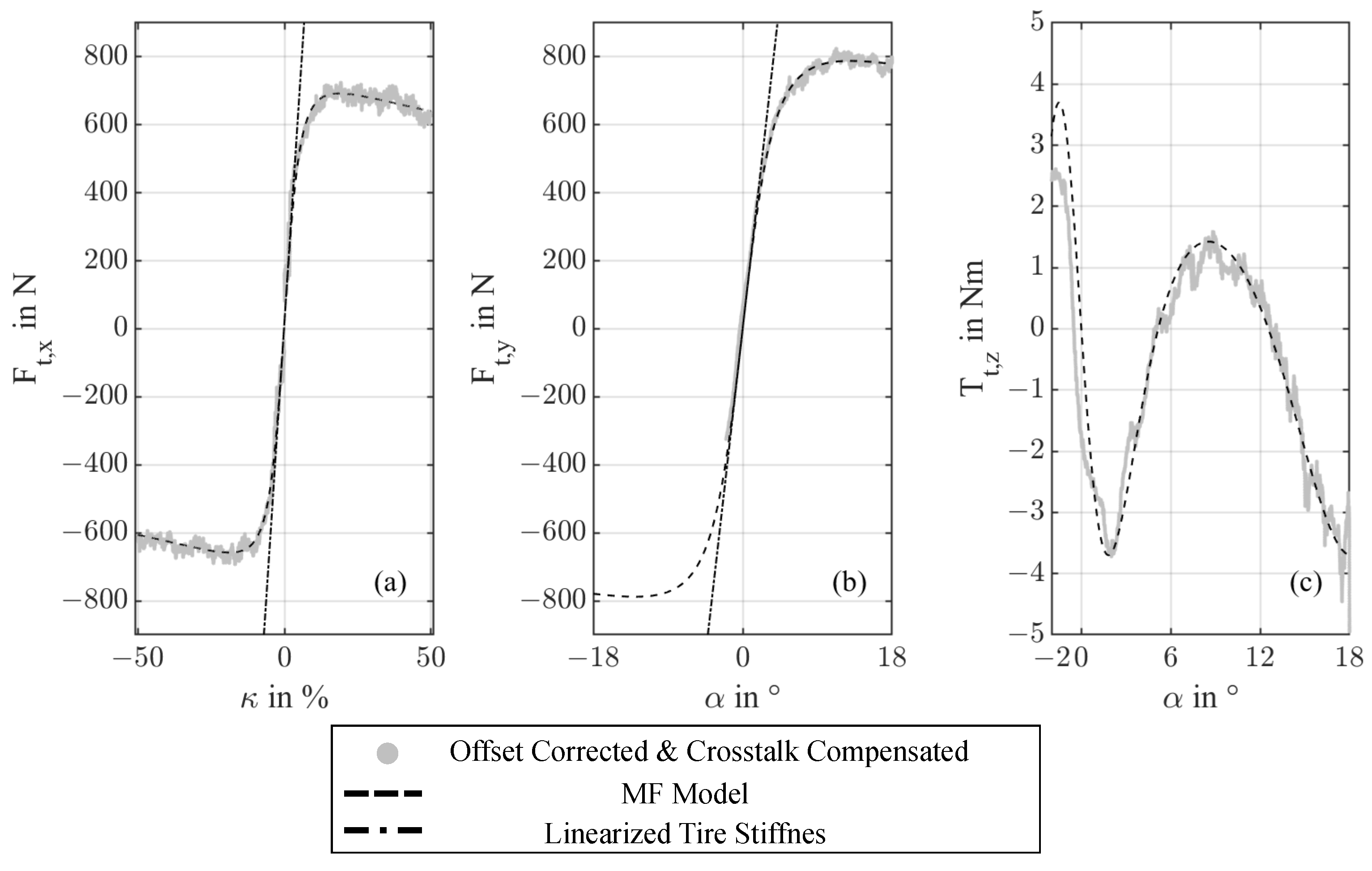
Figure 6 presents the data of test no. 3.1. The diagram is divided into the results of the acceleration and braking tests that cover $F_{t,x}\left(\kappa \right)$, which are listed in Figure 6a. The results of the steering test are shown in (b) as $F_{t,y}\left(\alpha \right)$ and (c) shows the relation $T_{t,z}\left(\alpha \right)$.

In a first step, the raw data are analyzed more closely, which is visualized as a black point cloud and shows a large scatter for $F_{t,x}\left(\kappa \right)$, $F_{t,y}\left(\alpha \right)$ and $T_{t,z}\left(\alpha \right)$. This results, in part, from the not exactly reproducible environmental conditions, such as the asphalt condition, tire wear or the temperature. In addition, there is a fluctuation in the contact force $F_{N,z}$ that the test truck exerts on the tire. The pneumatic adjustment of the contact force must be repeated after each tire change. A noticeable behavior can be seen in diagram (c), which shows the drift of the raw $T_{t,z}$ data when the slip angle $\alpha$ is larger than 8${}^{°}$. It is assumed that the crosstalk of the measurement system is responsible for this effect, since investigations according to [16] specify a different shape of the base curve of $T_{t,z}$. In contrast to the base curve, which generally has two zero crossings and a minimum in-between, only one zero crossing and a subsequent drifting of the $T_{t,z}$ curve in the direction of $-\infty$, as can be observed in the raw data. The proof of this assumption is provided by the crosstalk correction described later in this section. After its application, the $T_{t,z}$ data show a second zero-crossing and a minimum between the first and second zero-crossing, as can be seen in Figure 6c. To draw conclusions about the real behavior of the tire from the data, the offset of the measurement system is compensated first. Within the scope of the offset correction, an attempt is made to compensate the measurement error of the system which results, for example, from hysteresis. For this purpose, load-free conditions are set before and after each measurement series, so the unloaded condition offset of the force channels can be measured. Resulting offset values for test no. 3.1 are listed in

Table 2. Captured force outputs before and after measurement series for test no. 3.1.

Test Case	Force Channel	Force before Test in N	Force after Test in N
drive	$F_x$	−5.875	−4.491
	$F_y$	5.702	−106.491
	$F_z$	−2.891	11.616
brake	$F_x$	−11.230	−5.473
	$F_y$	−0.397	−27.325
	$F_z$	−8.052	14.288
steer	$F_x$	−5.180	−0.403
	$F_y$	3.108	−85.590
	$F_z$	−0.890	32.541

. The recorded offsets of $F_{t,x}$, $F_{t,y}$ and $T_{t,z}$ before and after the measurement series of one test case, e.g., driving for test no. 3.1 are used to calculate a straight line passing through the offset points. Subsequently, this straight line is subtracted from the measurement data. Offset-corrected and RLOWESS smoothed data are represented in Figure 6 as a dark gray point cloud. Since the offset data are recorded for the force sensors, but not for the measurement of torque, diagram (c) does not show an offset-corrected dataset. The offset still existing after the compensation, especially for the measurements of $F_{t,y}$ and $T_{t,z}$, results from a default setting of $\alpha$ and $\gamma$ of the measurement equipment, which is not exactly at 0${}^{°}$. A more precise setup of these parameters is not possible.

Compared to the raw data, the offset-corrected data of $F_{t,x}$ and $F_{t,y}$ show a similar linear trend at the beginning. However, with the beginning of the non-linear range at $\kappa$ ≥ 4% or $\alpha$ ≥ 5${}^{°}$, the deviation of the graphs increases. At this point, the offset corrected graphs exceed the mean of the raw data. This behavior is particularly clear when looking at $F_y$ for $\alpha$ ≥ 12${}^{°}$. Considering Table 2, this behavior can be explained as the offset measurement of $F_y$ after the test case “steer” is far below 0 N. The same applies to all other axes, whose values after the test cases deviate further from 0 N than the values measured before the test case. Further, $F_{t,x}$ and $F_{t,y}$ show an oscillatory force characteristic for the ranges $\kappa$ > 15% and, respectively, $\alpha$ > 8${}^{°}$ in the nonlinear region.

As already explained, it can be assumed that the measurement system suffers from crosstalk. For this reason, test measurements were carried out to identify the crosstalk and its effects. By applying an increasing force in the x-direction, whether all other channels show a change as well or whether they remain unchanged is unexamined. The results of the investigation are shown in Figure 7.

As can be seen from Figure 7, all other channels except $T_{t,x}$ show increasing or decreasing behavior, which rises with a higher force in x-direction, although they should not undergo a significant force or torque change. For this reason, the confirmed crosstalk is compensated.

Measurements with the MoReLab are normally made with a measurement rim with an offset of 60 mm, so the use of the adapter rim with an offset of 5 mm results in a different behavior, with a crosstalk effect that has to be corrected. For this reason, the crosstalk of the force and torque measurements is evaluated more closely in the subsequent section. Since [22] describes similar effects for this kind of measurement device, the method he described for crosstalk compensation of force sensors is also used in the proposed research. Therefore, according to [22], a correction matrix K is created by applying a defined force in one direction, while the effects on all other channels that measure forces and torques are recorded. The introduced force or torque is applied via an adapter that geometrically corresponds to the adapter rim, so that all existing lever ratios that will appear during the tire measurements are considered. The procedure is carried out on all axes by applying a force, followed by a defined torque on all axes. Because the measurement hub of the test truck does not have a brake and is only driven by a hydraulic driveshaft, the torque of the y-axis cannot be measured. For this reason, the correction matrix of [22] is reduced by one column and one row. The objective is to determine the effects that the introduction of a static force or torque to adapter rims geometry have on the measurements of the remaining axes. From uncorrected tire measurements, a maximum force of 1000 N and a maximum torque of 15 Nm can be expected. Based on these expected values, a slightly larger input force and torque were used in these experiments to cover the range needed for the tire measurements. The input forces and torques, as well as the resulting output values on all other channels, can be seen in

Table 3. Crosstalk measurements.

		Input
		${\mathit{F}}_{\mathit{x}}$ in N [1203]	${\mathit{F}}_{\mathit{y}}$ in N [1222]	${\mathit{F}}_{\mathit{z}}$ in N [1200]	${\mathit{T}}_{\mathit{x}}$ in Nm [305]	${\mathit{T}}_{\mathit{z}}$ in Nm [−25]
Output	$F_x$ in N	1165.781	22.869	−51.702	46.202	−10.975
	$F_y$ in N	−32.988	1124.557	16.104	28.154	19.211
	$F_z$ in N	−38.956	−13.866	1235.548	−63.938	2.544
	$T_x$ in Nm	1.665	13.150	3.433	292.221	0.599
	$T_z$ in Nm	8.318	0.058	−4.131	−14.675	−25.366

.

Subsequently, the correction matrix K was obtained from the crosstalk data listed in Table 3 by dividing each output value of a column by the applied input force or torque.

$$K=\left(\begin{array}{ccccc}0.969& 0.019& -0.043& 0.152& 0.430\\ -0.027& 0.920& 0.013& 0.092& -0.753\\ -0.032& -0.011& 1.029& -0.210& -0.010\\ 0.001& 0.011& 0.003& 0.959& -0.023\\ 0.007& 0.0000476& -0.003& -0.048& 0.995\end{array}\right)$$

(7)

Finally, the inverse of the $5\times 5$ correction matrix K was determined to solve Equation (8). Matrix O is defined as the $5\times 1$ raw data matrix and X as the final and crosstalk-compensated $5\times 1$ output matrix.

$$X=K^{-1}·O$$

(8)

The crosstalk compensated and RLOWESS smoothed data are shown as a purple point clouds in Figure 6. The crosstalk correction slightly raises the curve in $F_{t,x}$ and $F_{t,y}$ compared to the pure offset-compensated data. The most significant effect of the crosstalk correction is visible on the curve of $T_{t,z}$. While $T_{t,z}$ shows a strong drift before the crosstalk correction, the behavior after the correction corresponds to the base curve of [16] with a zero crossing around $\alpha$ = 0${}^{°}$ and $\alpha$ = 5${}^{°}$. In addition, the processed $T_{t,z}$ data have a minimum location between the first and second zero-crossing at around $\alpha$ = 2.5${}^{°}$. While the base curve after [16] shows an asymptotic approximation for high slip angles, this cannot be observed even in the crosstalk-compensated data from the present investigations. One explanation for this is the detachment of the tire casing from the rim at high slip angles, which was observed during the tests. Compared to car or truck tires that are used without an inner tube, tires with an inner tube can exhibit this behavior without losing pressure. In the crosstalk-compensated data, the effect is reflected at values of $\alpha$ > 10${}^{°}$. The resulting impact on the shear stress distribution in the contact area of the tire causes nonlinear effects, which lead to new reductions in $T_{t,z}$ for $\alpha$ > 13${}^{°}$. These effects have not yet been analyzed in detail within this framework, but they exhibit a fundamentally different behavior than tubeless car or truck tires. Since a tire slip from −50% to 50% and a slip angle from −2${}^{°}$ to 18${}^{°}$ were used in the measurements, the saturation of the tire for $F_{t,x}$ and $F_{t,y}$ is clearly visible in Figure 6. Therefore, data quality is only obtained after post-processing obtained, which allows for a realistic modeling on the basis of the collected data.

3.2. Observations during the Measurement

During the test campaign, some noticeable findings were observed that contain:

• Loose spokes of the adapter rim after steering measurements;
• High tire abrasion after steering measurements;
• Thin high-temperature line on the tire surface.

When measuring $F_{t,y}$ and $T_{t,x}$ an increased occurrence of slightly loose spokes in the rim during the steering measurement series was observed. A possible explanation for this effect is based on the assumption that bicycle rims are developed for driving with higher camber angles; the high $\alpha$ values with $\gamma$ = 0${}^{°}$ during the measurements can bend the rim. As a consequence, the spokes can be stressed by compressive forces even though they are optimized for tensile forces. The compressive force can relieve the spoke nipples and, consequently, the threads, which can then be loosened by oscillations in the system, as seen in Figure 6b for $\alpha$ > 6${}^{°}$. The spokes were checked after each series of measurements and tightened if necessary.

Due to the high loads during the bicycle tire tests, a high level of tire abrasion was noticed. As the used tires do not have a mark for replacement, they were used until the tire tread was completely worn away. The complete removal of the tread by a series of measurements can be seen in Figure 8a. Figure 8b shows a tire that was overstressed as the internal mesh became visible. Measurements made with overstressed tires were not included in the evaluation, since the detached tread of the tire has a strong impact on the adhesion values.

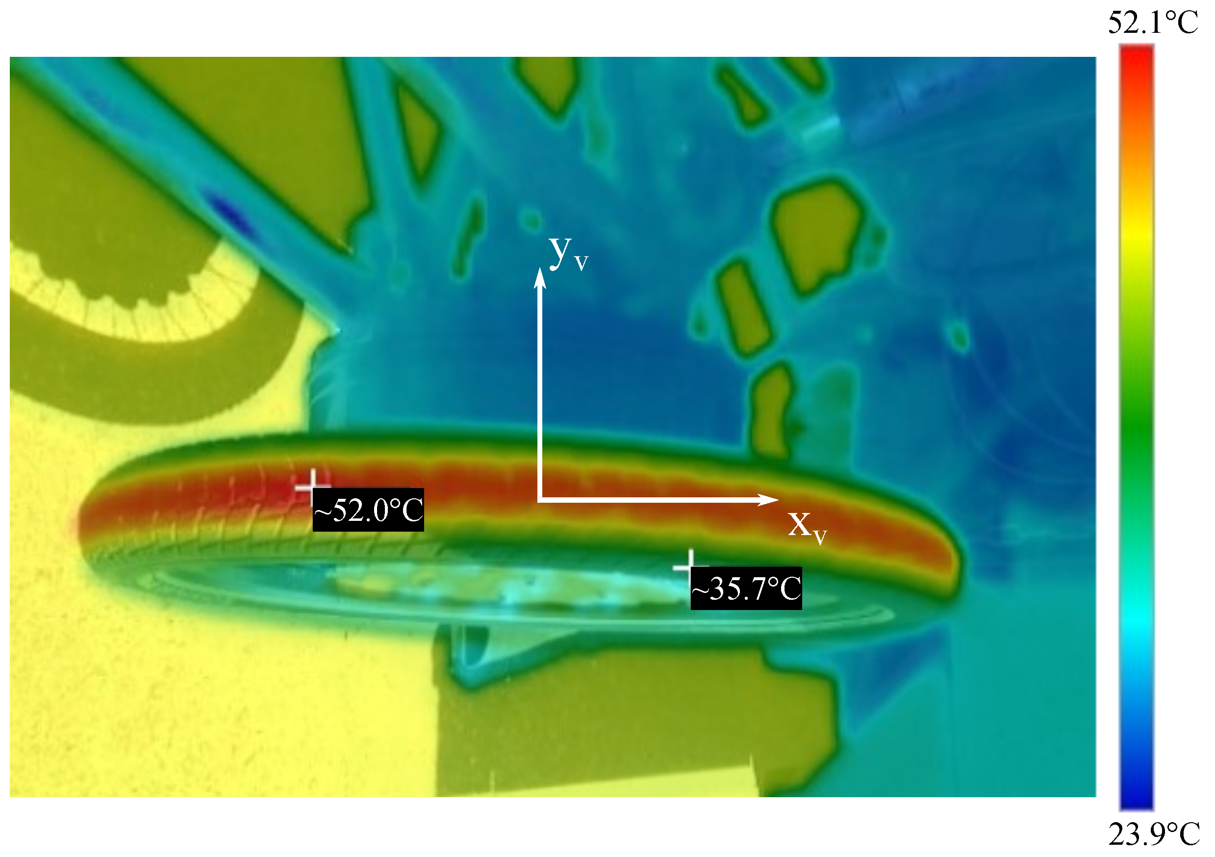
In order to evaluate the temperature behavior of the tires more accurately, the image shown in Figure 9 was obtained after a series of 18 steering measurements with the aid of a thermal imaging camera. As can be seen from the Figure, a thin line forms in the center of the tire, which reaches temperatures of approx. 52 °C. After a slim transition layer, the tire reaches a temperature of approx. 36 °C at the edge. Since the tire is driven without any camber angle, there is little to no friction at the edge areas of the tire. The local heat zones thus correspond to the overstressed tire tread shown in Figure 8b. Furthermore, the thermal imaging can ensure that a new tire survives a measurement series of 18 measurements without excessive temperatures. The tire image in Figure 8b is, therefore, the result of excessive testing.

3.3. Tire Modeling

The modeling of the tire behavior according to Equation (4) was carried out using the offset-compensated, crosstalk-corrected and RLOWESS-averaged data. The coefficients were optimized using the non-linear least squares method with the aid of the trust region algorithm, so that the model fit the data as accurately as possible. Since the model represents both $F_{t,x}\left(\kappa \right)$, $F_{t,y}\left(\alpha \right)$ and $T_{t,z}\left(\alpha \right)$ the coefficients carried the following indices i:

• x for MF coefficients used to model $F_{t,x}\left(\kappa \right)$;
• y for MF coefficients used to model $F_{t,y}\left(\alpha \right)$;
• z for MF coefficients used to model $T_{t,z}\left(\alpha \right)$.

A modified form of Equation (4) was further recommended according to [16] for modeling $T_{t,z}\left(\alpha \right)$. This involves replacing the sine function in Equation (4) with a cosine function, which results in a different shape of the curve that has proved to have more accuracy when fitting the measured values of $T_{t,z}\left(\alpha \right)$.

The resulting equation is given by:

$$y=D·cos(C·arctan(B·x-E·(B·x-arctan(B·x\left)\right)\left)\right)$$

(9)

Thus, $F_{t,x}\left(\kappa \right)$ and $F_{t,y}\left(\alpha \right)$ were subsequently modeled using Equation (4), while the model of $T_{t,z}\left(\alpha \right)$ was created using Equation (9). Furthermore, the longitudinal and lateral stiffness of the tires $C_{f,\kappa }$ and $C_{f,\alpha }$ can be obtained from the MF coefficients after fitting the models with:

$$C_{f,\kappa }=B_x·C_x·D_x$$

(10)

and:

$$C_{f,\alpha }=B_y·C_y·D_y$$

(11)

After post-processing of the measurement data, a small offset and shift was still present. For the measurements of $F_{t,x}\left(\kappa \right)$ the vertical offset was caused by the rolling resistance. Therefore, a horizontal shift of the model was accepted during optimization via the parameter $S_V,x$. Since no ply-steer and conicity effects are expected for a bicycle tire, the parameter $S_H,x$ was not considered and remains at 0.

However, the not precisely adjustable zero position of the slip angle ${\alpha }_0$ = 0${}^{°}$ of the test truck leads to a shift in the post-processed data of the $F_{t,y}\left(\alpha \right)$ and $T_{t,z}\left(\alpha \right)$ measurements. Furthermore, the lever arm discussed in Section 2.1.1 can result in an unintended torque around the z-axis, which leads to the elastic deformation of the fixture of the measurement wheel shown on Figure 10. As a result of the errors mentioned above, the angle ${\alpha }_0$ iwa affected by means of ${\alpha }_0$ ≠ 0${}^{°}$.

The average horizontal shift error ${\overline{e}}_{h,F_y}$ of all tests due to misalignments of ${\alpha }_0$ at $\alpha$ = $0^{°}$ for $F_{t,y}\left(\alpha \right)$ results in 1.2%. The horizontal shift error ${\overline{e}}_{h,T_z}$ due to misalignment of ${\alpha }_0$ at $\alpha$ = 0${}^{°}$ for $T_{t,z}\left(\alpha \right)$ is given as 1.7% compared to the full scale angle of 20${}^{°}$. Despite the described error, the model that is to be developed is supposed to follow the physical conformity of tires with $\gamma$ = 0${}^{°}$. Based on this consideration, the modeling of $F_{t,y}\left(\alpha \right)$ and $T_{t,z}\left(\alpha \right)$ is carried out with the conditions $F_{t,y}\left(0^{°}\right)$ = 0 N and $T_{t,z}\left(0^{°}\right)$ = 0 Nm, although ${\overline{e}}_{h,F_y}$ and ${\overline{e}}_{h,T_z}$ are slightly visible in the data. As a consequence, the MF coefficients $S_H,y$ and $S_V,y$ for the model of $F_{t,y}\left(\alpha \right)$ resulted in a fixed value of 0. Due to the cosine function in Equation (9), a small shift must be allowed to maintain $T_{t,z}\left(0^{°}\right)$ = 0 Nm, to provide an optimal fit of the model to the data. Therefore, the coefficient $S_V,z$ was limited to 0 for the modeling of $T_{t,z}\left(\alpha \right)$, while $S_H,z$ ≠ 0 allowed a small shift to achieve a zero transition at $T_{t,z}\left(0^{°}\right)$. The models created under these boundary conditions for test no. 3.1 are shown in Figure 11, while the

Table 4. Magic formula coefficients and model fit for $F_{t,x}\left(\kappa \right)$.

Test No.	${\mathit{B}}_{\mathit{x}}$	${\mathit{C}}_{\mathit{x}}$	${\mathit{D}}_{\mathit{x}}$	${\mathit{E}}_{\mathit{x}}$	${\mathit{S}}_{\mathit{H}},\mathit{x}$	${\mathit{S}}_{\mathit{V}},\mathit{x}$	R2	NRMSE
1.1	0.133	1.364	678.7	0.000	0.000	−36.080	0.996	0.026
1.2	0.094	1.700	892.4	0.665	0.000	−17.260	0.998	0.018
2.1	0.108	1.640	663.4	0.680	0.000	−42.600	0.997	0.023
2.2	0.105	1.436	826.9	0.122	0.000	−57.670	0.997	0.023
3.1	0.121	1.611	675.2	0.713	0.000	−17.170	0.998	0.018
3.2	0.067	2.146	831.1	0.982	0.000	−12.100	0.999	0.015

,

Table 5. Magic formula coefficients and model fit for $F_{t,y}\left(\alpha \right)$.

Test No.	${\mathit{B}}_{\mathit{y}}$	${\mathit{C}}_{\mathit{y}}$	${\mathit{D}}_{\mathit{y}}$	${\mathit{E}}_{\mathit{y}}$	${\mathit{S}}_{\mathit{H}},\mathit{y}$	${\mathit{S}}_{\mathit{V}},\mathit{y}$	R2	NRMSE
1.1	0.210	1.412	774.0	0.633	0.000	0.000	0.995	0.017
1.2	0.127	1.373	1045.0	0.409	0.000	0.000	0.999	0.009
2.1	0.250	1.119	789.7	−0.461	0.000	0.000	0.994	0.019
2.2	0.123	1.542	922.1	0.388	0.000	0.000	0.998	0.011
3.1	0.174	1.561	788.1	0.618	0.000	0.000	0.993	0.020
3.2	0.161	1.216	912.0	0.397	0.000	0.000	0.997	0.015

and

Table 6. Magic formula coefficients and model fit for $T_{t,z}\left(\alpha \right)$.

Test No.	${\mathit{B}}_{\mathit{z}}$	${\mathit{C}}_{\mathit{z}}$	${\mathit{D}}_{\mathit{z}}$	${\mathit{E}}_{\mathit{z}}$	${\mathit{S}}_{\mathit{H}},\mathit{z}$	${\mathit{S}}_{\mathit{V}},\mathit{z}$	R2	NRMSE
1.1	0.185	7.715	3.600	1.340	1.150	0.000	0.941	0.061
1.2	0.082	9.000	4.397	1.717	2.200	0.000	0.969	0.047
2.1	0.189	7.442	3.500	1.339	1.160	0.000	0.912	0.065
2.2	0.101	8.381	4.000	1.607	1.910	0.000	0.937	0.058
3.1	0.126	8.611	3.700	1.627	1.490	0.000	0.902	0.074
3.2	0.128	7.572	4.200	1.441	1.680	0.000	0.905	0.072

show the MF coefficients as well as the models normalized root mean squared error (NRMSE) for all tests that were carried out. The normalization of the root mean squared error (RMSE) was performed with respect to the range of measured values described by Equation (12).

$$NRMSE=\frac{RMSE}{y_{max}-y_{min}}$$

(12)

Depending on the case, y must be replaced by $F_{t,x}$, $F_{t,y}$ or $T_{t,z}$. The data and figures for the remaining tests can be found in [18].

As can be seen from Figure 11, with respect to Table 4, Table 5 and Table 6, it is possible to fit the measured and post-processed data of a bicycle tire with the MF Equations (4) and (9). The model of $F_{t,y}$ allows for the representation of $F_{t,y}\left(\alpha \right)$ for $\alpha$ < −2${}^{°}$. The model of $T_{t,z}$ was only plotted for $\alpha$ values from −2${}^{°}$ to 18${}^{°}$. This results from the modeling of $T_{t,z}\left(\alpha \right)$ using Equation (9), which shows no symmetric behavior for the coefficients that were used. For this reason, $T_{t,z}\left(\alpha \right)$ must be intersected, inverted and flipped at $\alpha$ = 0${}^{°}$ to obtain a model of $T_{t,z}\left(\alpha \right)$ in the range $\alpha$ < 0${}^{°}$. The calculated coefficients used to model $F_{t,x}\left(\kappa \right)$, $F_{t,y}\left(\alpha \right)$, and $T_{t,z}\left(\alpha \right)$, as well as the goodness of fit of the models, are shown in Table 4, Table 5 and Table 6. As can be seen from the tables, by optimizing the coefficients, it is possible to model all measured values of the six tests using the MF model with an R² value > 0.9. Therefore, the choice of coefficients results in a suitable model quality.

With respect to the NRMSE, minimum and maximum values from 0.009 to 0.074 indicate an overall good model fit. A larger error of $F_{t,x}\left(\kappa \right)$ than $F_{t,y}\left(\alpha \right)$ can be obtained for most cases. This effect results from the sharpness of the measured curves of $F_{t,x}$, which will lead to difficulties in modeling with the coefficients B, C, D and E. Reference [16] refers to the introduction of a new parameter H in an extra term of Equation (4), whereby the sharpness of the curve can be modeled more accurately. Since a basic MF model was used in the present research, this parameter is not considered. Slightly increased values of the NRMSE for the goodness of fit of the model of $T_{t,z}\left(\alpha \right)$ result from the described shift in the measured data, which was corrected by the boundary conditions during modeling. In addition, Equation (9) of the MF model used is capable of representing even the missing asymptotic behavior for large slip angles, as shown in Figure 11 for $\alpha$ > 10${}^{°}$.

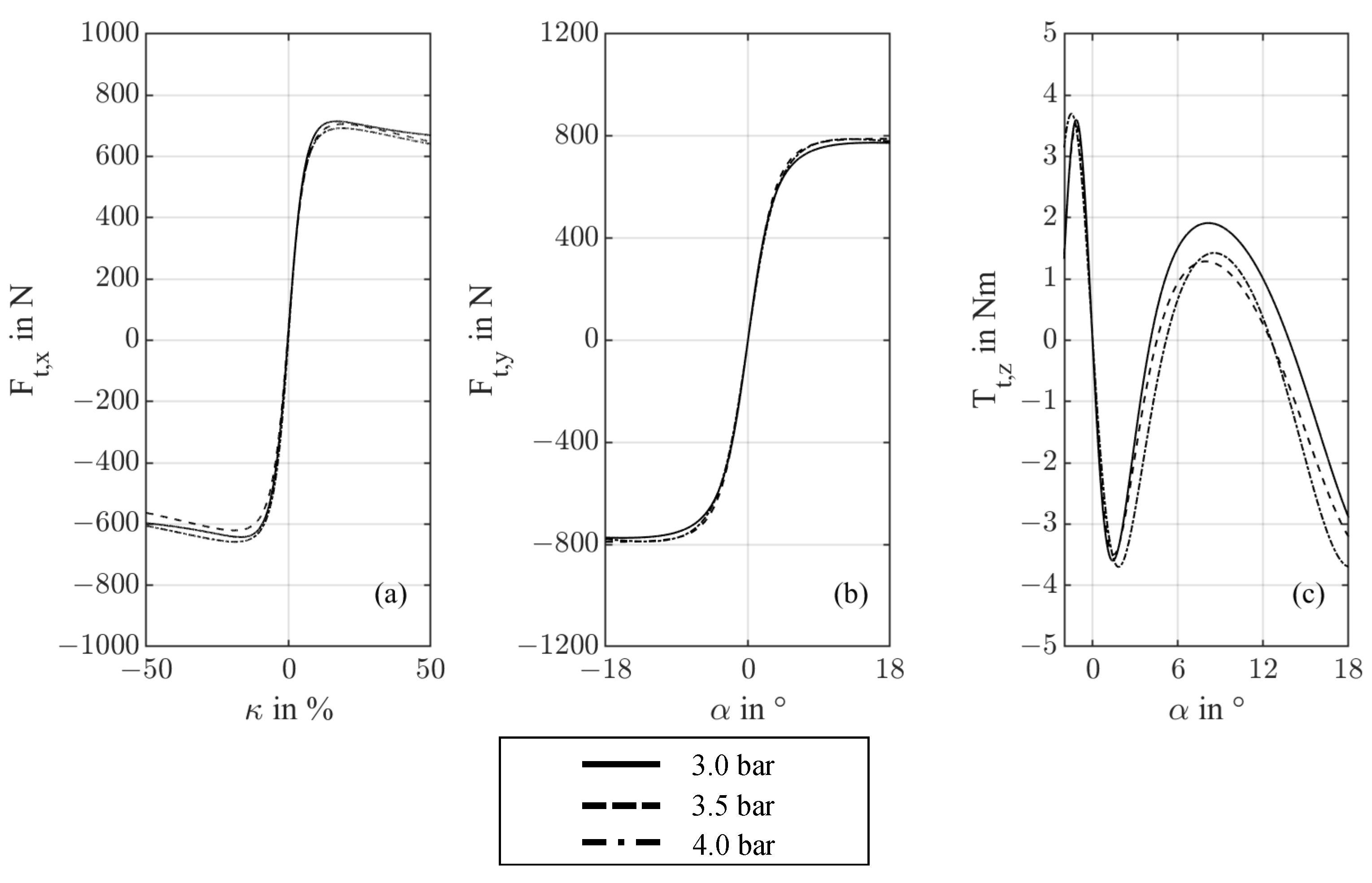
3.4. Impact of Tire Pressure and Normal Force

To investigate the impact of tire pressure on the measurements, Figure 12 shows the model curves of $F_{t,x}\left(\kappa \right)$, $F_{t,y}\left(\alpha \right)$ and $T_{t,z}\left(\alpha \right)$ at a normal force of 625 N and tire pressures of 3.0, 3.5 and 4.0 bar. As can be seen from (a), (b) and (c) in Figure 12, a change from 1 bar to the tire pressure only had a minor effect on the maximum transmittable longitudinal and lateral forces, as well as the aligning torque of the bicycle tire tested when $F_{N,z}$ = 625 N. In addition, the slope of the models in the linear range remains almost the same.

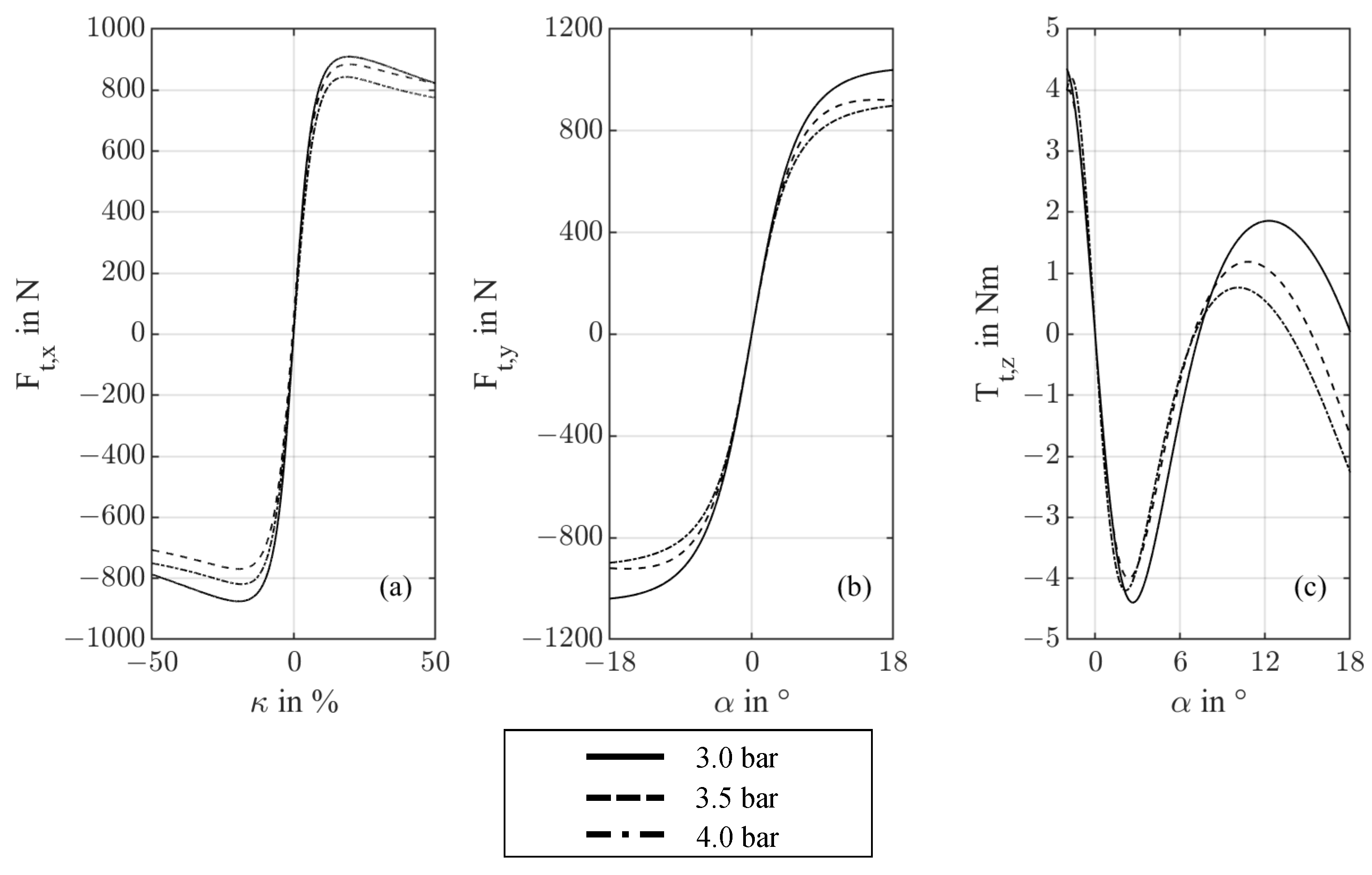
The impact of changing the tire pressure from 3 bar to 4 bar in steps of 0.5 bar on the longitudinal and lateral forces $F_{t,x}\left(\kappa \right)$ and $F_{t,y}\left(\alpha \right)$ as well as the aligning torque $T_{t,z}\left(\alpha \right)$ at $F_{N,z}$ = 765 N is shown in Figure 13.

Compared with the measurements at $F_{N,z}$ = 625 N, a contact force of $F_{N,z}$ = 765 N results in a significantly larger spread of the force curves $F_{t,x}$ and $F_{t,y}$ in the range of $\kappa$ > 10% and $\alpha$ > 4${}^{°}$ at different tire pressures. Furthermore, the three-bar model curve can reach the highest force values in both the longitudinal and lateral direction. However, the four-bar curve produces the lowest force values in both directions. By comparing the curves of $F_{N,z}$ = 625 N and $F_{N,z}$ = 765 N, it is clear that the effects of different tire pressures are more significant for a higher value of $F_{N,z}$. For example, by comparing $\Delta F_{t,x,p}$ = $F_{t,x,3bar}-F_{t,x,4bar}$ at $\kappa$ = 25% for $F_{N,z}$ = 625 N and $F_{N,z}$ = 765 N. $\Delta F_{t,x,p}$ results in 17.6 N for $F_{N,z}$ = 625 N. $\Delta F_{t,x,p}$ for $F_{N,z}$ = 765 N results in 70 N. The effect is more significant when looking at $\Delta F_{t,y,p}$ = $F_{t,y,3bar}-F_{t,y,4bar}$ at $\alpha$ = 9${}^{°}$ and $F_{N,z}$ = 625 N as well as $F_{N,z}$ = 765 N. $\Delta F_{t,y,p}$ for $F_{N,z}$ = 625 N results in 21.8 N $\Delta F_{t,y,p}$ at $F_{N,z}$ = 765 N reaches 118.6 N. It is assumed that the wire-reinforced carcass of the bicycle tire prevents a significant increase in the contact area when the tire pressure is reduced. A larger tire contact area is achievable at higher values for $F_{N,z}$, which results in a higher transmittable longitudinal and lateral force. Therefore, the effects of the tire pressure are only slightly visible on the model curves of the $F_{N,z}$ = 625 N, but are clearly visible in the model curves of $F_{N,z}$ = 765 N. Ref. [23] describes a similar effect for the behavior of scooter tires. Ref. [24] describes an opposite behavior for high-performance motorcycle tires, but refers to the dependence on the construction of the tire if this effect is observed.

4. Discussion

Within the scope of the present investigations, bicycle tires for cargo trailers were measured with the help of the MoReLab on real road surface conditions on the test track at Vauffelin. It was shown that the test truck, whose regular purpose is the automotive sector, is capable of measuring the behavior of bicycle tires. Due to the rim design and the dimensions of bicycle tires and wheels, an adapter rim had to be used for the measurements, which does not allow for the same positioning of the wheel compared to car or truck tires. As a result, a lever arm was introduced that led to crosstalk effects, which needed to be corrected. It could be shown that the crosstalk can be compensated using the method of [22], so that the measurement data of $T_{t,z}\left(\alpha \right)$ follow the base curve according to [16]. Due to inaccuracies in setting the zero position of the slip angle as well as the occurring lever arm, a small measurement error arose in the measurements of $F_{t,y}\left(\alpha \right)$ and $T_{t,z}\left(\alpha \right)$ in the case of horizontal shift. A correction was made during modeling by selecting the boundary conditions. Within modeling, the MF according to [16] was used, and its coefficients were determined by optimization. Due to the described shift, boundary conditions for the coefficients are defined in such a way that the models corresponded to the physical theory. Since the slip angle $\alpha$ can be set from −2${}^{°}$ to 18${}^{°}$ using the test truck, the measurements for the positive range of $\alpha$ visualize the saturation of the tire. The experiments complement the investigations according to [14], which cover a smaller slip angle range, although these were carried out for a different tire type and the use of the camber angle $\gamma$.

To improve the modeling accuracy of $F_{t,x}$ and to reduce the slightly increased RMSE, the MF coefficient H according to [16] can be used in further analyses to improve the sharpness of the curve. The influence of the tire pressure could be investigated at different normal forces. The lower normal force $F_{N,z}$ was limited by the test system, so that the intended lower normal force of 500 N could not be adjusted. For further investigations, a second analysis at a lower normal force than 625 N would be appropriate in this context. At a contact force of 765 N, the tire pressure had a significant influence on the maximum transmittable longitudinal and lateral forces. In contrast, the change in the gradient of the linear range at the same normal force was small. We plan to investigate the impact of tire pressure on the longitudinal and lateral forces by a subsequent analysis of the contact area. Further, it should to be noted that the present investigations were carried out with a camber angle of $\gamma$ = 0${}^{°}$. If the presented models are used for the simulation of a bicycle, e.g. a cargo bike, the impact of camber on the longitudinal and lateral forces must be taken into account. Ref. [13] provides detailed information regarding this behavior.

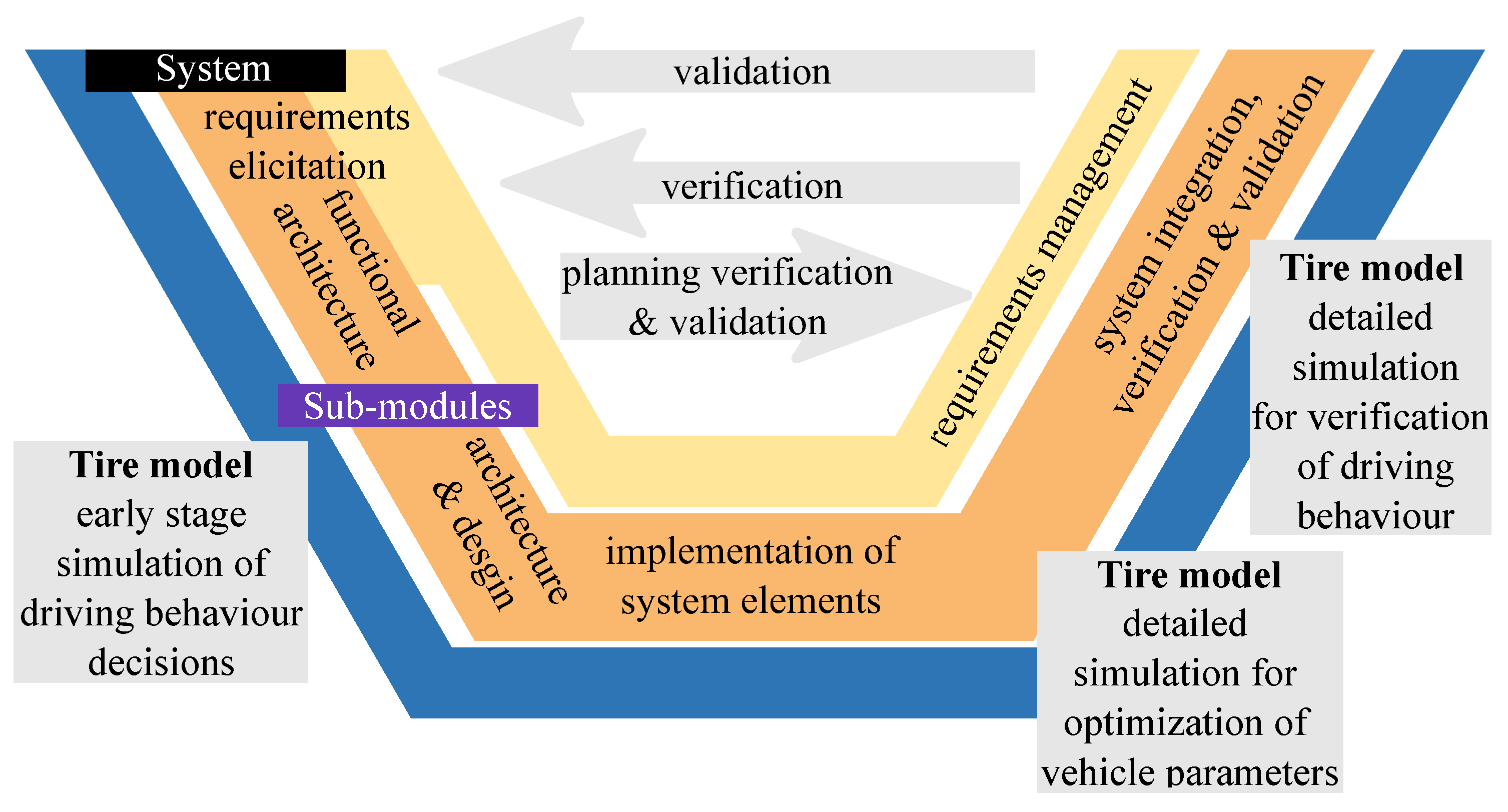
An essential aspect of tire modeling within the development of the drive control of an electrically propelled bicycle trailer is made clear by integration into the V-model. At oresent, most product development processes generally follow the principles of model-based systems engineering (compare, e.g., VDI 2206 [25,26]). This means that models continuously accompany the entire processes and are used for simulation for verification and validation purposes. In industrial companies, current product development processes usually apply model-based systems engineering (MBSE). The inherent procedural logics in such processes can be depicted in a so-called V-model (compare VDI 2206 [25]) and can be seen in Figure 14.

The main logical path in a V-model shows the progression from the requirements (e.g., permissible cargo weight) formulated for one technical system (e.g., a cargo bicycle trailer) over the intermediate steps such as the implementation of system elements to the final realization of the system. In systematic MBSE, the different stages are supported by appropriate algorithms, methods and tools and the different product and process models are interconnected. The requirements elicitation is supported by means of model-based requirements engineering [27]. In the development of the product architecture, the engineers can be supported by integrated function modelling [28,29], abstract physics representations [30], connected domain-specific models [31], integrated verification processes [32] and automated parameter selection approaches [33]. For novel products such as bike trailers with a supporting drive system, the tire behavior is very important for the sensible simulation of both the longitudinal and lateral dynamic behavior. Such simulations are carried out throughout the product development process, e.g., for the continuous refinement of vehicle parameters. These refinements are needed for the safety and fault-tolerance of the system, i.e., if driver faults lead to sudden direction changes (compare [34]). In Figure 14, three main objectives of simulations based on tire models are shown. In their early phases, such simulations can be used to support concept decisions. In later stages, they are used for the tuning of other vehicle parameters, such as spring rates. Finally, the verification of the driving behavior of the complete system can also rely on such simulations.

5. Conclusions

The measurement of bicycle tires for cargo trailers was carried out in accordance with the requirements for such vehicles with the aid of a mobile tire test laboratory on asphalt and under real ambient conditions. Parameters such as tire pressure and contact force were changed within an expected range so that their effects could be recorded. Occurring crosstalk was compensated by means of a correction matrix, so that only after the correction was performed did the curve of $T_{t,z}\left(\alpha \right)$ correspond to the typical behavior of a tire according to [16]. By setting up suitable boundary conditions, the modeling process ensured that the models to be developed followed the physical principles and that small measurement errors were corrected. It has been shown that the general form of the MF, listed in Equation (4), is suitable for modeling the measured data. For future investigations, other forms of the MF can be used to generate models that already include p and $F_{N,z}$ as input. In comparison, the tire at a lower normal force of 625 N showed a slight change in the behavior of $F_{t,x}\left(\kappa \right)$, $F_{t,y}\left(\alpha \right)$ and $T_{t,z}\left(\alpha \right)$, while at a normal force of 765 N, a significant influence of the tire pressure on $F_{t,x}\left(\kappa \right)$, $F_{t,y}\left(\alpha \right)$ and $T_{t,z}\left(\alpha \right)$ was observed. The models can subsequently be used for the further design of a control system for an electrically driven trailer with the purpose of load transportation.

References

- Carla Cargo: Products—eCarla. Available online: https://www.carlacargo.de/de/produkte/ecarla/ (accessed on 14 July 2022).
- Nüwiel: ProductP. Available online: https://www.nuwiel.com/etrailer/ (accessed on 14 July 2022).
- Kyburz: Products—DXP. Available online: https://kyburz-switzerland.ch/en (accessed on 14 July 2022).
- Heißing, B.; Schimmel, C. Fahrverhalten. In Fahrwerkhandbuch; Ersoy, M., Gies, S., Eds.; Springer Vieweg Wiesbaden: Wiesbaden, Germany, 2017; pp. 202–203. [Google Scholar]
- Korayem, A.H.; Khajepour, A.; Fidan, B. A Review on Vehicle-Trailer State and Parameter Estimation. IEEE T-ITS 2022, 23, 5993–6010. [Google Scholar]
- Vempaty, S.; He, Y. A Review of Car-Trailer Lateral Stability Control Approaches; SAE Technical Paper 2017-01-1580. In Proceedings of the WCX™ 17: SAE World Congress, Detroit, MI, USA, 4 April 2017. [Google Scholar]
- Isermann, R. Tire Traction and Force Transfer. In Automotive Control; ATZ/MTZ-Fachbuch; Springer: Berlin/Heidelberg, Germany, 2022. [Google Scholar]
- Guiggiani, M. Mechanics of the Wheel with Tire. In The Science of Vehicle Dynamics; Springer: Cham, Switzerland, 2023. [Google Scholar]
- Vempaty, S.; Lee, E.; He, Y. Model-Reference Based Adaptive Control for Enhancing Lateral Stability of Car-Trailer Systems. In Proceedings of the ASME 2016 International Mechanical Engineering Congress and Exposition, Phoenix, AZ, USA, 7 March 2016. [Google Scholar]
- Shamim, R.; Islam, M.M.; He, Y. A Comparative Study of Active Control Strategies for Improving Lateral Stability of Car-Trailer Systems. In Proceedings of the SAE 2011 World Congress & Exhibition, Detroit, MI, USA, 14 April 2011. [Google Scholar]
- Frey, M.; Gnadler, R.; Guenter, F. Untersuchung der Verlustleistung an Pkw-Reifen. Proc. Reifen Fahrwerk Fahrb. Tag. 1995, 10, 101–128. [Google Scholar]
- Eckert, M. Energieoptimale Fahrdynamikregelung Mehrmotoriger Elektrofahrzeuge; KIT Scientific Publishing: Karlsruhe, Germany, 2015. [Google Scholar] [CrossRef]
- Dressel, A.E. Measuring and Modeling the Mechanical Properties of Bicycle Tires. Master’s Thesis, University of Wisconsin-Milwaukee, Milwaukee, WI, USA, May 2013. [Google Scholar]
- Dressel, A.; Sadauckas, J. Characterization and Modelling of Various Sized Mountain Bike Tires and the Effects of Tire Tread Knobs and Inflation Pressure. Appl. Sci. 2020, 10, 3156. [Google Scholar] [CrossRef]
- Doria, A.; Tognazzo, M.; Cusimano, G.; Bulsink, V.; Cooke, A.; Koopman, B. Identification of the mechanical properties of bicycle tyres for modelling of bicycle dynamics. Veh. Syst. Dyn. 2012, 51, 405–420. [Google Scholar] [CrossRef]
- Pacejka, H.B.; Besselink, I. Tire and Vehicle Dynamics, 3rd ed.; Butterworth-Heinemann: Oxford, UK, 2012. [Google Scholar]
- Schwalbe Pick-Up. Available online: https://www.schwalbe.com/en/tour-reader/schwalbe-pick-up (accessed on 20 July 2022).
- Miller, M.; Pfeil, M.; Reick, B.; Murri, R.; Stetter, R.; Kennel, R. Measurement Data of Longitudinal and Lateral Behaviour of a Bicycle Tire for Cargo Trailers. Dataset; Technical University of Munich: Munich, Germany, 2022. [Google Scholar] [CrossRef]
- Bakker, E.; Nyborg, L.; Pacejka, H.B. Tyre Modelling for Use in Vehicle Dynamics Studies. SAE Trans. 1987, 96, 190–204. [Google Scholar]
- Besselink, I.J.M.; Schmeitz, A.J.C.; Pacejka, H.B. An improved Magic Formula/Swift tyre model that can handle inflation pressure changes. In Proceedings of the 21st Symposium of the International Association for Vehicle System Dynamics (IAVSD 09), Stockholm, Sweden, 17–21 August 2009; pp. 337–352. [Google Scholar] [CrossRef]
- Blundell, M.; Harty, D. Multibody Systems Approach to Vehicle Dynamics, 2nd ed.; Elsevier: Amsterdam, The Netherlands, 2015. [Google Scholar] [CrossRef]
- Schrand, D. Cross-Talk Compensation Using Matrix Methods. Sens. Transducers J. 2007, 5, 1157–1163. [Google Scholar]
- Cossalter, V.; Doria, A.; Lot, R.; Ruffo, N.; Salvador, M. Dynamic Properties of Motorcycle and Scooter Tires: Measurement and Comparison. Veh. Syst. Dyn. 2003, 39, 329–352. [Google Scholar] [CrossRef]
- Massaro, M.; Cossalter, V.; Cusimano, G. The effect of the inflation pressure on the tyre properties and the motorcycle stability. Proc. Inst. Mech. Eng. Part J. Automob. Eng. 2013, 10, 1480–1488. [Google Scholar] [CrossRef]
- VDI/VDE 2206 Entwurf. In Entwicklung Cyber-Physischer Mechatronischer Systeme (CPMS); Beuth: Berlin, Germany, 2020.
- Gräßler, I.; Hentze, J. The new V-Model of VDI 2206 and its validation. At-Automatisierungstechnik 2020, 68, 312–324. [Google Scholar] [CrossRef]
- Holder, K.; Zech, A.; Ramsaier, M.; Stetter, R.; Niedermeier, H.P.; Rudolph, S.; Till, M. Model-based requirements management in gear systems design based on graph-based design languages. Appl. Sci. 2017, 7, 1112. [Google Scholar] [CrossRef] [Green Version]
- Eisenbart, B.; Gericke, K.; Blessing, L.T.; McAloone, T.C. A DSM-based framework for integrated function modelling: Concept, application and evaluation. Res. Eng. Des. 2017, 28, 25–51. [Google Scholar] [CrossRef] [Green Version]
- Elwert, M.; Ramsaier, M.; Eisenbart, B.; Stetter, R.; Till, M.; Rudolph, S. Digital Function Modeling in Graph-Based Design Languages. Appl. Sci. 2022, 12, 5301. [Google Scholar] [CrossRef]
- Stetter, R. Approaches for Modelling the Physical Behavior of Technical Systems on the Example of Wind Turbines. Energies 2020, 13, 2087. [Google Scholar] [CrossRef]
- Shaked, A.; Reich, Y. Using Domain-Specific Models to Facilitate Model-Based Systems-Engineering: Development Process Design Modeling with OPM and PROVE. Appl. Sci. 2021, 11, 1532. [Google Scholar] [CrossRef]
- Laing, C.; David, P.; Blanco, E.; Dorel, X. Questioning integration of verification in model-based systems engineering: An industrial perspective. Comput. Ind. 2020, 114, 103163. [Google Scholar] [CrossRef]
- Lu, J.; Chen, D.; Wang, G.; Kiritsis, D.; Törngren, M. Model-Based Systems Engineering Tool-Chain for Automated Parameter Value Selection. IEEE Trans. Syst. Man Cybern. Syst. 2021, 52, 2333–2347. [Google Scholar] [CrossRef]
- Stetter, R. Fault-Tolerant Design and Control of Automated Vehicles and Processes, 1st ed.; Springer: Cham, Germany, 2020. [Google Scholar] [CrossRef]
Figure 1.
MoReLab truck and measurement chamber with mounted bicycle tire and corresponding coordinate system.
Figure 2.
Overview of measurement and drive control system.
Figure 3.
Measurement hub with offsets of bicycle rim and tire (a) yz-plane view (b) xy-plane view (c) xy-plane view with .
Figure 4.
Tested tire (a) mounted on adapter rim (b) view of the profile.
Figure 5.
Post-processing chain.
Figure 6.
Measured and post-processed data of test no. 3.1 where (a) shows , (b) shows and (c) shows .
Figure 7.
Crosstalk according to input .
Figure 8.
Tire wear according to the measurements where (a) has a replaceable but acceptable tire condition, while (b) has been overstressed.
Figure 9.
Thermal image of a tire after measuring the steering case with approx. 18 measurements in xy-plane view.
Figure 10.
Wheel fixture deformation according to lever arm where (a) shows the optimal case with no error of and (b) shows an elastic deformation with .
Figure 11.
Post-processed data and MF Model of test no. 3.1, where (a) shows , (b) shows and (c) shows .
Figure 12.
MF Models of Test no. 1.1, 2.1 and 3.1 where (a) shows , (b) shows and (c) shows .
Figure 13.
MF Models of Test no. 1.2, 2.2 and 3.2 where (a) shows , (b) shows and (c) shows .
Figure 14.
V-model: electrified bicycle trailer control.