Differentiation of the Wright Functions with Respect to Parameters and Other Results

Abstract

In this work, we discuss the derivatives of the Wright functions (of the first and the second kinds) with respect to parameters. The differentiation of these functions leads to infinite power series with the coefficients being the quotients of the digamma (psi) and gamma functions. Only in few cases is it possible to obtain the sums of these series in a closed form. The functional form of the power series resembles those derived for the Mittag-Leffler functions. If the Wright functions are treated as generalized Bessel functions, differentiation operations can be expressed in terms of the Bessel functions and their derivatives with respect to the order. In many cases, it is possible to derive the explicit form of the Mittag-Leffler functions by performing simple operations with the Laplacian transforms of the Wright functions. The Laplacian transform pairs of both kinds of Wright functions are discussed for particular values of the parameters. Some transform pairs serve to obtain functional limits by applying the shifted Dirac delta function. We expect that the present analysis would find several applications in physics and more generally in applied sciences. These special functions of the Mittag-Leffler and Wright types have already found application in rheology and in stochastic processes where fractional calculus is relevant. Careful readers can benefit from the new results presented in this paper for novel applications.

1. Introduction

The partial differential equations of a fractional order are successively applied for modelling time and space diffusion, stochastic processes, probability distributions, and other diverse natural phenomena. They are extremely important in physical processes that can be described by using fractional calculus. In the mathematical literature, when a solution of these fractional differential equations is desired, we frequently encounter the Wright functions, named after him. In 1933 [1] and 1940 [2], these functions were considered to be a generalization of the Bessel functions; however, today, they play a significant independent role in the theory of special functions. There are many investigations devoted to the analytical properties and applications of the Wright functions, but only two survey papers are mentioned here, in which essential material on the subject is included [3,4]. These functions are particular cases of higher transcendental functions, as recently shown in interesting surveys by Kiryakova [5] and Srivastava [6].

In this paper, we discuss three quite different subjects that are associated with the Wright functions. In the first part, the Wright function $W_{\alpha ,\beta }\left(t\right)$ where t is the argument, and $\alpha$ and $\beta$ are the parameters, is differentiated with respect to the parameters, and derived expressions are compared with similar formulas for the Mittag-Leffler functions. With continuous effort, after investigating the differentiation of the Bessel and Mittag-Leffler functions with respect to their parameters [7,8,9], this mathematical operation is extended here to the Wright functions. Special attention is devoted to the cases when the Wright functions can be reduced to Bessel functions and expressed in a closed form. Auxiliary functions $F_{\alpha }\left(t\right)$ and $M_{\alpha }\left(t\right)$, which were introduced for the first time in the 1990s by Mainardi [4] and are now called the Mainardi functions, are also discussed in this section.

The functional behaviour of derivatives with respect to the order is also presented in graphical form. The presented plots were prepared by evaluating the sums of infinite series by using the MATHEMATICA programme.

The second part of this paper is dedicated to the Laplacian transform pairs of the Wright functions. It is demonstrated how the Laplacian transforms of the Wright functions are useful in obtaining explicit expressions for the Mittag-Leffler functions. Lastly, we discuss the functional limits that are associated with the Wright and the Mittag-Leffler functions. These limits can be derived by applying the delta sequence in the form of the shifted Dirac function. This delta sequence is directly related to the order of Bessel function and was introduced by Lamborn in 1969 [8,9,10,11,12,13,14].

Throughout this paper, all mathematical operations or manipulations with functions, series, integrals, integral representations, and transforms are formal, and it was assumed that the arguments and parameters are real numbers. There are no proofs of the validity of the derived results, though they were presumed to be correct considering that they were in part previously obtained independently with other methods.

2. Wright Functions of the First and Second Kinds

Wright functions $W_{\alpha ,\beta }\left(z\right)$ are defined with the series representation as a function of complex argument z, and parameters $\alpha$ and $\beta$.

$$W_{\alpha ,\beta }\left(z\right)=\sum _{k=0}^{\infty }\frac{z^k}{k!\Gamma (\alpha k+\beta )}.$$

(1)

They are entire functions of $z\in \mathbb{C}$ for $\alpha >-1$ and for any complex $\beta$ (here always $\beta \ge 0$). According to Mainardi (see Appendix F of [4]), we distinguish the Wright function of the first kind for $\alpha \ge 0$, and of the second kind for $-1<\alpha <0$. This distinction is justified for the difference in the asymptotic representations in the complex domain and in the Laplacian transforms for a real positive argument. For our purposes, we recall their Laplacian transforms for positive argument t. We have, by using the symbol ÷ to denote the juxtaposition of a function $f\left(t\right)$ with its Laplacian transform $\tilde{f}\left(s\right)$, for the first kind, when $\alpha \ge 0$

$$W_{\alpha ,\beta }(\pm t)÷\frac{1}{s}{E}_{\lambda ,\mu }\left(\pm \frac{1}{s}\right);$$

(2)

for the second kind, when $-1<\alpha <0$ and putting for convenience $\nu =-\alpha$ so $0<\nu <1$

$$W_{-\nu ,\beta }(-t)÷E_{\nu ,\beta +\nu }\left(-s\right).$$

(3)

Above, we introduced the Mittag-Leffler function in two parameters $\alpha >0$, $\beta \in \mathbb{C}$ defined as its convergent series for all $z\in \mathbb{C}$

$$E_{\alpha ,\beta }\left(z\right):=\sum _{k=0}^{\infty }\frac{z^k}{\Gamma (\alpha k+\beta )}.$$

(4)

For more details on the special functions of the Mittag-leffler type, we refer the interested readers to the treatise by Gorenflo et al. [7], where in the recent second edition, the Wright functions are also treated in some detail.

3. Differentiation of the Wright Functions of the First Kind with Respect to Parameters

We first compare the Wright functions of the first kind with the two-parameter Mittag-Leffler functions for $\alpha >0$ and $\beta \ge 0$, from which they differ only by the absence of factorials.

The direct differentiation of the series with respect to the $\alpha$ parameter gives

$$\begin{array}{c}\frac{\partial W_{\alpha ,\beta }\left(t\right)}{\partial \alpha }=-{\sum }_{k=1}^{\infty }\left(\frac{\psi (\alpha k+\beta )}{k!\Gamma (\alpha k+\beta )}\right)k{t}^k=\hfill \\ -{\sum }_{k=1}^{\infty }\left(\frac{\psi (\alpha k+\beta )}{(k-1)!\Gamma (\alpha k+\beta )}\right)t^k\hfill \\ \frac{\partial E_{\alpha ,\beta }\left(t\right)}{\partial \alpha }=-{\sum }_{k=1}^{\infty }\left(\frac{\psi (\alpha k+\beta )}{\Gamma (\alpha k+\beta )}\right)k{t}^k\hfill \end{array}$$

(5)

and with respect to the $\beta$ parameter

$$\begin{array}{c}\frac{\partial W_{\alpha ,\beta }\left(t\right)}{\partial \beta }=-{\sum }_{k=0}^{\infty }\left(\frac{\psi (\alpha k+\beta )}{k!\Gamma (\alpha k+\beta )}\right)t^k\hfill \\ \frac{\partial E_{\alpha ,\beta }\left(t\right)}{\partial \beta }=-{\sum }_{k=0}^{\infty }\left(\frac{\psi (\alpha k+\beta )}{\Gamma (\alpha k+\beta )}\right)t^k\hfill \end{array}$$

(6)

The second derivatives are

$$\begin{array}{c}\frac{{\partial }^2{W}_{\alpha ,\beta }\left(t\right)}{\partial {\alpha }^2}={\sum }_{k=1}^{\infty }\left\{\frac{{\left[\psi (\alpha k+1)\right]}^2-{\psi }^{\left(1\right)}(\alpha k+\beta )}{k!\Gamma (\alpha k+\beta )}\right\}k{}^2{t}^k\hfill \\ \frac{{\partial }^2{E}_{\alpha ,\beta }\left(t\right)}{\partial {\alpha }^2}={\sum }_{k=1}^{\infty }\left\{\frac{{\left[\psi (\alpha k+1)\right]}^2-{\psi }^{\left(1\right)}(\alpha k+\beta )}{\Gamma (\alpha k+\beta )}\right\}k{}^2{t}^k\hfill \end{array}$$

(7)

and

$$\begin{array}{c}\frac{{\partial }^2{W}_{\alpha ,\beta }\left(t\right)}{\partial {\beta }^2}={\sum }_{k=0}^{\infty }\left\{\frac{{\left[\psi (\alpha k+\beta )\right]}^2-{\psi }^{\left(1\right)}(\alpha k+\beta )}{k!\Gamma (\alpha k+\beta )}\right\}{t}^k\hfill \\ \frac{{\partial }^2{E}_{\alpha ,\beta }\left(t\right)}{\partial {\beta }^2}={\sum }_{k=0}^{\infty }\left\{\frac{{\psi (\alpha k+\beta )]}^2-{\psi }^{\left(1\right)}(\alpha k+\beta )}{\Gamma (\alpha k+\beta )}\right\}{t}^k\hfill \end{array}$$

(8)

For the Mittag-Leffler and Wright functions, we have the same functional expressions, but in the case of the Wright functions, factorials appear. Contrary to the Mittag-Leffler functions [9,10], the summation of these series by using MATHEMATICA gives only few results in a closed form in terms of the following generalized hypergeometric functions:

$$\begin{array}{c}\frac{\partial W_{\alpha ,\beta }\left(t\right)}{\partial \alpha }\left|{}_{\alpha =1,\beta =0}\right.=-{\sum }_{k=1}^{\infty }\left(\frac{\psi \left(k\right)}{{[(k-1)!]}^2}\right)t^k=t_0{F}_1(;1;t)\hfill \\ \frac{\partial W_{\alpha ,\beta }\left(t\right)}{\partial \alpha }\left|{}_{\alpha =1,\beta =1}\right.=-{\sum }_{k=1}^{\infty }\left(\frac{\psi (k+1)}{(k-1)!k!}\right)t^k=t_0{F}_1(;2;t)\hfill \end{array}$$

(9)

and

$$\begin{array}{c}\frac{\partial W_{\alpha ,\beta }\left(t\right)}{\partial \beta }\left|{}_{\alpha =1,\beta =0}\right.=-{\sum }_{k=0}^{\infty }\left(\frac{\psi \left(k\right)}{(k-1)!k!}\right)t^k=\hfill \\ \frac{1}{2}[t{}_0{F}_1(;1;t)-t{}_0{F}_1(;2;t)lnt]+\sqrt{t}{K}_1\left(2\sqrt{t}\right)\hfill \\ \frac{\partial W_{\alpha ,\beta }\left(t\right)}{\partial \beta }\left|{}_{\alpha =1,\beta =1}\right.=-{\sum }_{k=0}^{\infty }\left(\frac{\psi (k+1)}{{(k!)}^2}\right)t^k={}_0{F}_1(;1;t)\hfill \end{array}$$

(10)

In the last case, $\alpha =\beta =1$, in the Brychkov compilation of infinite series [15], the sum is expressed in terms of the following modified Bessel functions:

$$\begin{array}{c}\frac{\partial W_{\alpha ,\beta }\left(t\right)}{\partial \beta }\left|{}_{\alpha =\beta =1}\right.=-{\sum }_{k=0}^{\infty }\left(\frac{\psi (k+1)}{{(k!)}^2}\right)t^k=\hfill \\ -\frac{1}{2}lnt{I}_0\left(2\sqrt{t}\right)-K_0\left(2\sqrt{t}\right)\hfill \end{array}$$

(11)

Using the MATHEMATICA programme, the values of the derivatives with respect to parameters $\alpha$ and $\beta$ of the Wright functions of the first kind were calculated for the argument $0.25\le t\le 4.0$ and for parameters $0\le \alpha \le 5.0$ and $0\le \beta \le 2.0$.

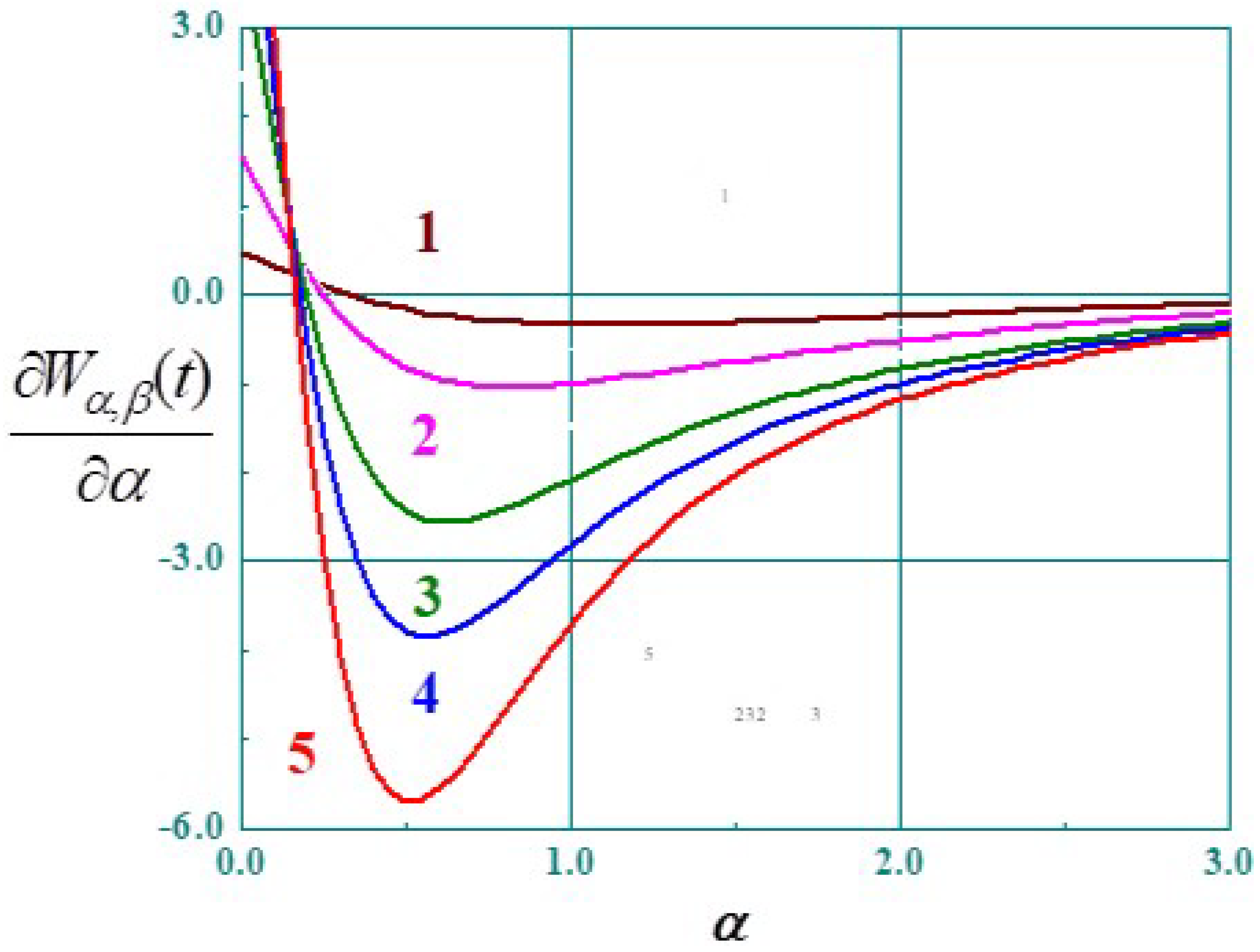
Figure 1 illustrates the behaviour of derivatives with respect to parameter $\alpha$ at different values of argument t.

In the $0<\alpha <1$ region, a minimum exists; with increasing $\alpha$, all curves tend to zero. The absolute value of the minimum increases with the increase in argument.

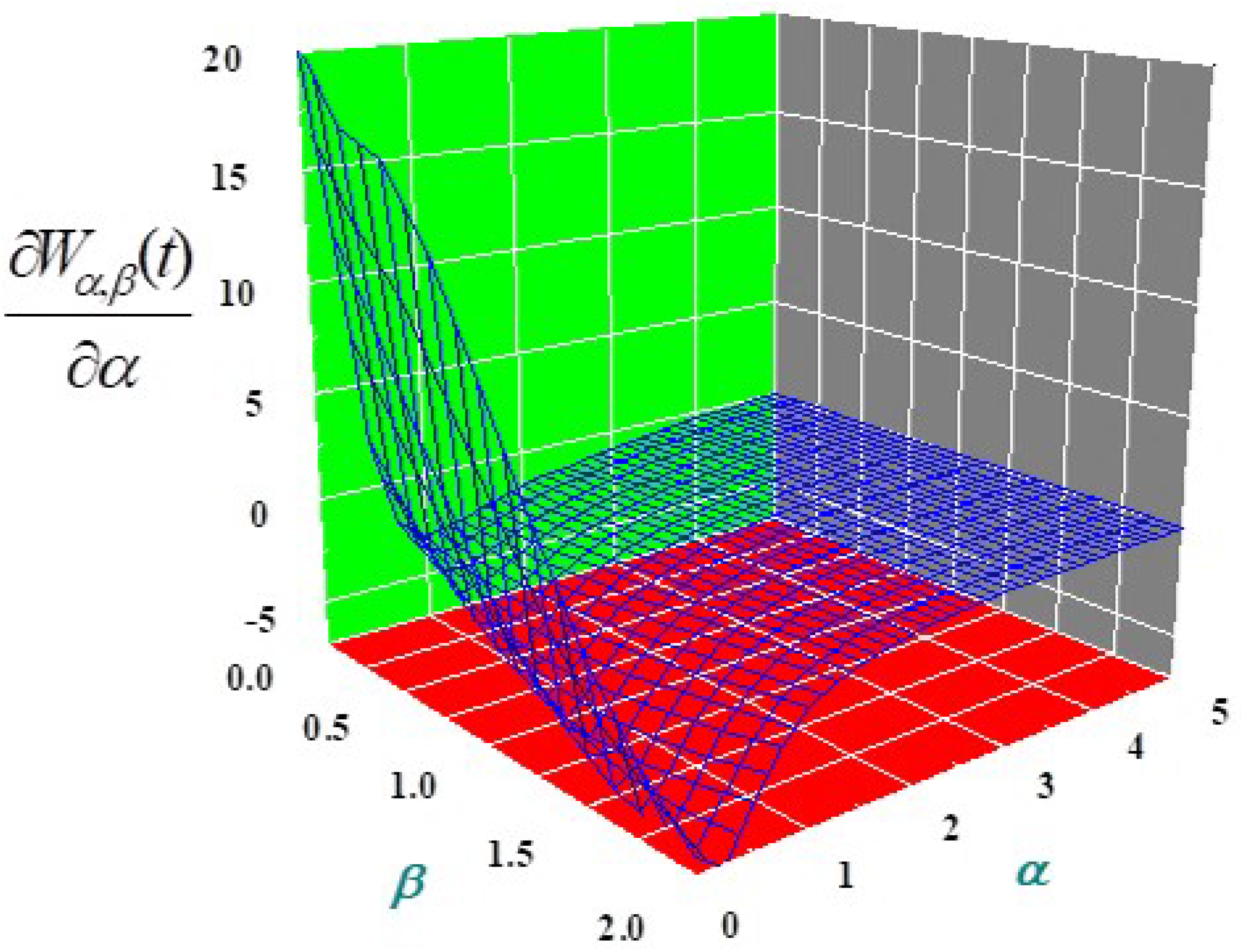
Derivatives with respect to parameters $\alpha$ and $\beta$ when the argument t is constant are presented in Figure 2. The functional form of the curves with the change in $\beta$ values is similar to that observed previously in Figure 1.

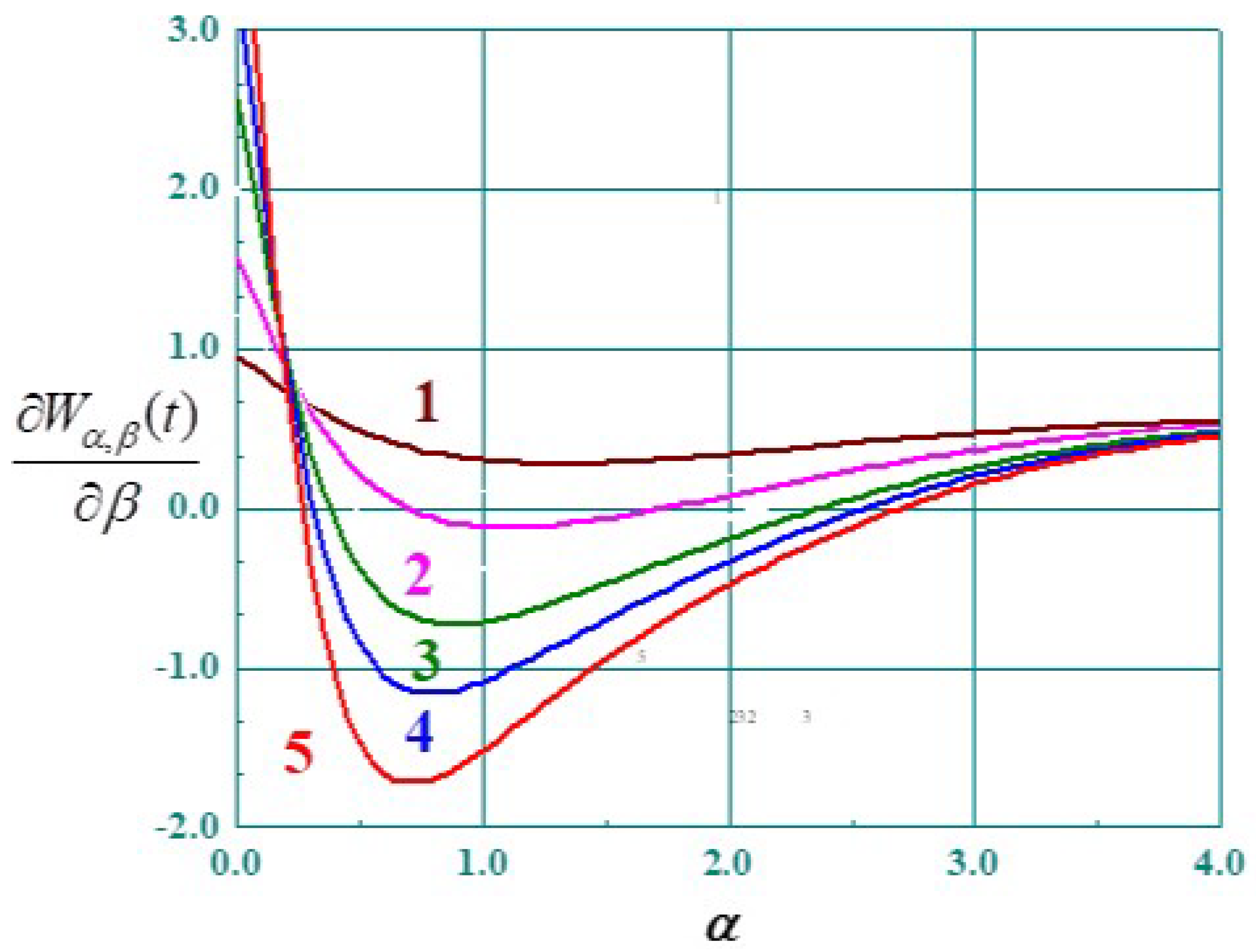
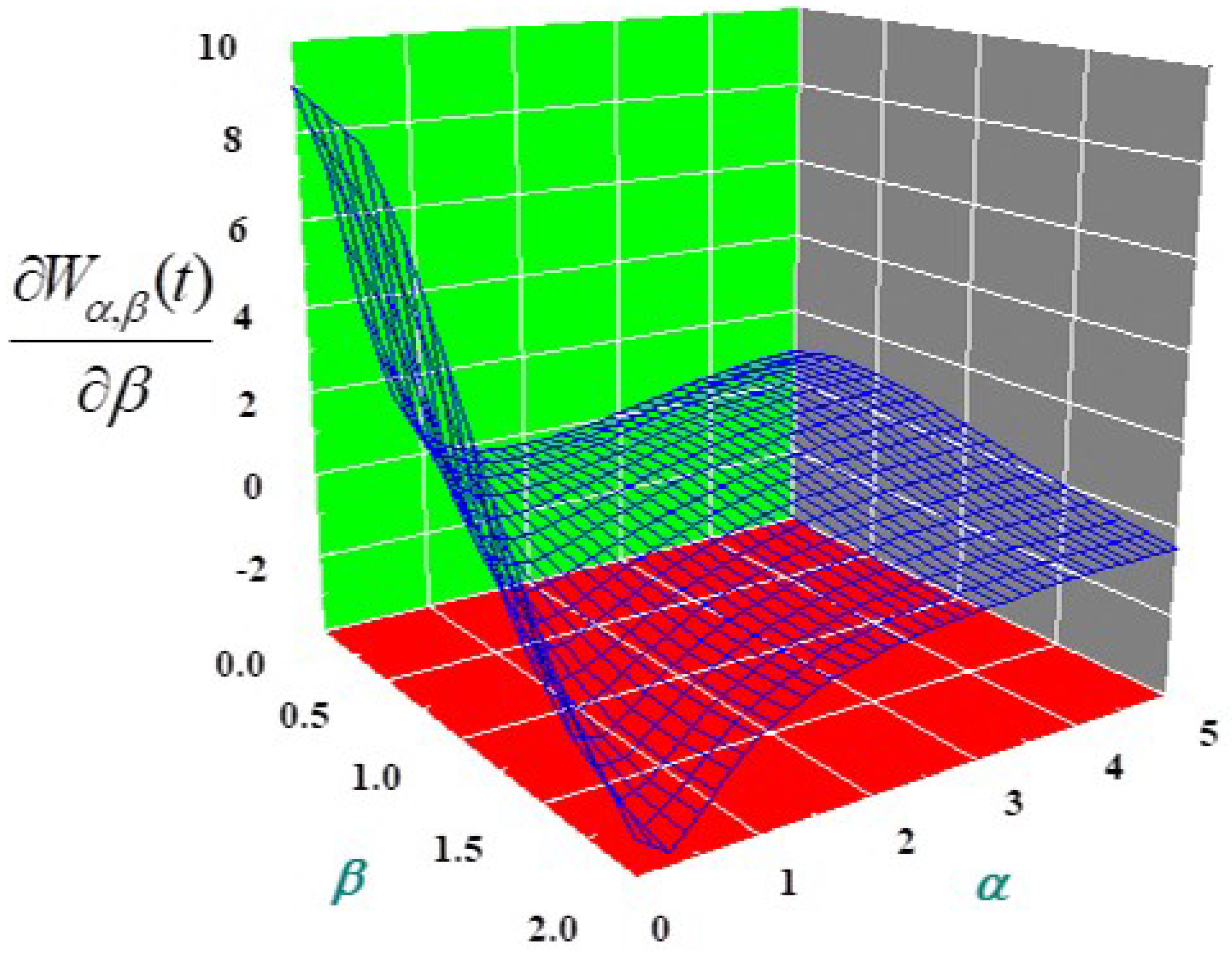
In order to compare the behaviour of the derivatives with respect to $\alpha$ with those with respect to $\beta$, the same conditions were imposed on t and $\beta$, as shown in Figure 1, Figure 2, Figure 3 and Figure 4. The similarity of the corresponding curves is evident, with the only difference being that the absolute values of the minima were lower for the derivatives with respect to parameter $\beta$ than that for $\alpha$.

4. Differentiation of the Wright Functions of the Second Kind with Respect to Parameters

We now consider, among the Wright functions of the second kind, functions, $F_{\alpha }\left(t\right)$ and $M_{\alpha }\left(t\right)$ introduced by Mainardi:

$$\begin{array}{c}{F}_{\alpha }\left(t\right)=W_{-\alpha ,0}\left(t\right);0<\alpha <1\hfill \\ M_{\alpha }\left(t\right)=W_{-\alpha ,1-}{}_{\alpha }\left(t\right);0<\alpha <1\hfill \\ F_{\alpha }\left(t\right)=\alpha t{M}_{\alpha }\left(t\right)\hfill \end{array}$$

(12)

Their series expansions explicitly read as follows:

$$F_{\alpha }\left(t\right)=\sum _{k=1}^{\infty }\frac{{(-t)}^k}{k!\Gamma (-\alpha k)}=-\frac{1}{\pi }\sum _{k=1}^{\infty }\frac{{(-t)}^k}{k!}\Gamma (\alpha k+1)sin\left(\pi \alpha k\right)$$

(13)

and

$$M_{\alpha }\left(t\right)=\sum _{k=0}^{\infty }\frac{{(-t)}^k}{k!\Gamma \left(-\alpha (k+1)+1\right)}=\frac{1}{\pi }\sum _{k=1}^{\infty }\frac{{(-t)}^{k-1}}{(k-1)!}\Gamma \left(\alpha k\right)sin\left(\pi \alpha k\right)$$

(14)

The direct differentiation of (13) and (14) gives

$$\begin{array}{c}\frac{\partial F_{\alpha }\left(t\right)}{\partial \alpha }=\frac{1}{\pi }{\sum }_{k=1}^{\infty }\frac{k{(-t)}^{k-1}}{k!}\Gamma (\alpha k+1)\left[\psi (\alpha k+1)sin\left(\pi \alpha k\right)+\pi cos\left(\pi \alpha k\right)\right]\hfill \\ \frac{\partial M_{\alpha }\left(t\right)}{\partial \alpha }=\frac{1}{\pi }{\sum }_{k=1}^{\infty }\frac{k{(-t)}^{k-1}}{(k-1)!}\Gamma \left(\alpha k\right)\left[\psi \left(\alpha k\right)sin\left(\pi \alpha k\right)+\pi cos\left(\pi \alpha k\right)\right]\hfill \end{array}$$

(15)

Using the last equation in (12), we have

$$\frac{\partial F_{\alpha }\left(t\right)}{\partial \alpha }=t{M}_{\alpha }\left(t\right)+\alpha t\frac{\partial M_{\alpha }\left(t\right)}{\partial \alpha }$$

(16)

The second derivatives of these functions are

$$\begin{array}{c}\frac{\partial {}^2{F}_{\alpha }\left(t\right)}{\partial {\alpha }^2}=\frac{1}{\pi }{\sum }_{k=1}^{\infty }\frac{k{(-t)}^{k-1}}{(k-1)!}\Gamma (\alpha k+1)\left\{[{\psi }^{\prime }(\alpha k+1)+\right.{\psi }^2(\alpha k+1)]sin\left(\pi \alpha k\right)+\hfill \\ 2\pi cos\left(\pi \alpha k\right)\psi (\alpha k+1)-\left.{\pi }^{2}sin\left(\pi \alpha k\right)\right\}\hfill \end{array}$$

(17)

and

$$\begin{array}{c}\frac{\partial {}^2{M}_{\alpha }\left(t\right)}{\partial {\alpha }^2}=\frac{1}{\pi }{\sum }_{k=1}^{\infty }\frac{k^2{(-t)}^{k-1}}{(k-1)!}\Gamma \left(\alpha k\right)\left\{[{\psi }^{\prime }\left(\alpha k\right)+\right.{\psi }^2\left(\alpha k\right)]sin\left(\pi \alpha k\right)+\hfill \\ 2\pi cos\left(\pi \alpha k\right)\psi \left(\alpha k\right)-\left.{\pi }^{2}sin\left(\pi \alpha k\right)\right\}\hfill \end{array}$$

(18)

They are interrelated by

$$\frac{{\partial }^2{F}_{\alpha }\left(t\right)}{\partial {\alpha }^2}=2t\frac{\partial M_{\alpha }\left(t\right)}{\partial \alpha }+\alpha t\frac{{\partial }^2{M}_{\alpha }\left(t\right)}{\partial {\alpha }^2}$$

(19)

5. Laplacian Transforms and the Wright Functions of the First Kind

The Laplacian transforms of the Wright functions are expressed in terms of the two-parameter Mittag-Leffler functions [3,4]:

$$L\left\{W_{\alpha ,\beta }(\pm \lambda t)\right\}=\frac{1}{s}{E}_{\alpha ,\beta }\left(\pm \frac{\lambda }{s}\right);\alpha >0;\lambda >0$$

(20)

Applying operational rules of the Laplacian transformation, we have [16,17,18]:

$$L\left\{e^{\pm \rho }{W}_{\alpha ,\beta }\left(\lambda t\right)\right\}=\frac{1}{s\mp \rho }{E}_{\alpha ,\beta }\left(\frac{\lambda }{s\mp \rho }\right);\lambda ,\rho >0$$

(21)

and this permits to obtain

$$\begin{array}{c}L\left\{sinh\left(\rho t\right)W_{\alpha ,\beta }\left(\lambda t\right)\right\}=\frac{1}{2}\left\{\frac{1}{s-\rho }{E}_{\alpha ,\beta }\left(\frac{\lambda }{s-\rho }\right)-\frac{1}{s+\rho }{E}_{\alpha ,\beta }\left(\frac{\lambda }{s+\rho }\right)\right\}\hfill \\ L\left\{cosh\left(\rho t\right)W_{\alpha ,\beta }\left(\lambda t\right)\right\}=\frac{1}{2}\left\{\frac{1}{s-\rho }{E}_{\alpha ,\beta }\left(\frac{\lambda }{s-\rho }\right)+\frac{1}{s+\rho }{E}_{\alpha ,\beta }\left(\frac{\lambda }{s+\rho }\right)\right\}\hfill \end{array}$$

(22)

Multiplication (20) by t gives

$$L\left\{t{W}_{\alpha ,\beta }\left(\lambda t\right)\right\}=-\frac{d}{ds}\left\{\frac{1}{s}{E}_{\alpha ,\beta }\left(\frac{\lambda }{s}\right)\right\}=-\left\{-\frac{1}{s^2}{E}_{\alpha ,\beta }\left(\frac{\lambda }{s}\right)+\frac{1}{s}\frac{d}{ds}{E}_{\alpha ,\beta }\left(\frac{\lambda }{s}\right)\right\}$$

(23)

The derivative of the Mittag-Leffler function is

$$\frac{d}{ds}{E}_{\alpha ,\beta }\left(\frac{\lambda }{s}\right)=-\frac{\lambda }{s^2}\left\{\frac{E_{\alpha ,\beta -1}\left(\frac{\lambda }{s}\right)-(\beta -1)E_{\alpha ,\beta }\left(\frac{\lambda }{s}\right)}{\alpha \left(\frac{\lambda }{s}\right)}\right\}$$

(24)

Lastly, we have

$$L\left\{t{W}_{\alpha ,\beta }\left(\lambda t\right)\right\}=\frac{1}{s^2}\left\{\frac{(\alpha \lambda -\beta +1)E_{\alpha ,\beta }\left(\frac{\lambda }{s}\right)+E_{\alpha ,\beta -1}\left(\frac{\lambda }{s}\right)}{\alpha \lambda }\right\}$$

(25)

In the case when the Wright functions are expressed as the Bessel functions (see (2.18)), the Laplacian transforms are known for $\beta =0,1,2$ [15]:

$$\begin{array}{c}{\int }_0^{\infty }{e}^{-st}{W}_{1,1}(-\frac{{\lambda }^2{t}^2}{4})dt={\int }_0^{\infty }{e}^{-st}{J}_0\left(\lambda t\right)dt=\frac{1}{\sqrt{s^2+{\lambda }^2}}\hfill \\ {\int }_0^{\infty }{e}^{-st}{W}_{1,2}(-\frac{{\lambda }^2{t}^2}{4})dt=\frac{2}{\lambda }{\int }_0^{\infty }{e}^{-st}\frac{J_1\left(\lambda t\right)}{t}dt=\frac{2}{[s+\sqrt{s^2+{\lambda }^2}]}\hfill \\ {\int }_0^{\infty }{e}^{-st}{W}_{1,3}(-\frac{{\lambda }^2{t}^2}{4})dt=\frac{4}{{\lambda }^2}{\int }_0^{\infty }{e}^{-st}\frac{J_2\left(\lambda t\right)}{t^2}dt=\hfill \\ \frac{1}{\lambda }\left\{\frac{\lambda }{[s+\sqrt{s^2+{\lambda }^2}]}+\frac{1}{3}{\left[\frac{\lambda }{[s+\sqrt{s^2+{\lambda }^2}]}\right]}^3\right\}\hfill \end{array}$$

(26)

From (A1), it follows that

$${\int }_0^{\infty }{e}^{-st}{W}_{1,\beta +1}(-\lambda t)dt=\frac{1}{{\lambda }^{\beta /2}}{\int }_0^{\infty }{e}^{-st}{t}^{-\beta /2}{J}_{\beta }\left(2\sqrt{\lambda t}\right)dt$$

(27)

and this integral equality is useful in deriving the explicit forms of the Mittag-Leffler functions. Starting with $\beta =0$, we have [19]

$${\int }_0^{\infty }{e}^{-st}{W}_{1,1}(-\lambda t)dt={\int }_0^{\infty }{e}^{-st}{J}_0\left(2\sqrt{\lambda t}\right)dt=\frac{1}{s}{e}^{-\lambda /s};Res>0$$

(28)

however, from (20),

$$L\left\{W_{1,1}(-\lambda t)\right\}=\frac{1}{s}{E}_{1,1}(-\frac{\lambda }{s})$$

(29)

Therefore, via comparison, the expected result is reached:

$$\begin{array}{c}{E}_{1,1}(-\frac{\lambda }{s})=e^{-\lambda /s}\hfill \\ \tau =\frac{\lambda }{s}\hfill \\ E_{1,1}(-\tau )=e^{-\tau }\hfill \end{array}$$

(30)

Introducing $\beta =1$ into (27), we have [19]

$$\begin{array}{c}{\int }_0^{\infty }{e}^{-st}{W}_{1,2}(-\lambda t)dt=\frac{1}{\sqrt{\lambda }}{\int }_0^{\infty }{e}^{-st}{t}^{-1/2}{J}_1\left(2\sqrt{\lambda t}\right)dt=\hfill \\ \sqrt{\frac{\pi }{\lambda s}}{e}^{-\lambda /2s}{I}_{1/2}\left(\frac{\lambda }{2s}\right)=\frac{2}{\lambda }{e}^{-\lambda /2s}sinh\left(\frac{\lambda }{2s}\right)=\frac{1}{\lambda }(1-e^{-\lambda /s})\hfill \\ {\int }_0^{\infty }{e}^{-st}{W}_{1,2}(-\lambda t)dt=\frac{1}{s}{E}_{1,2}(-\frac{\lambda }{s})\hfill \\ \tau =\frac{\lambda }{s}\hfill \\ E_{1,2}(-\tau )=\frac{1}{\tau }(1-e^{-\tau })\hfill \end{array}$$

(31)

In a general case, the Laplacian transform can be expressed in terms of the incomplete gamma function $\gamma (a,z)$ [15]:

$$\begin{array}{c}{\int }_0^{\infty }{e}^{-st}{W}_{1,\beta +1}(-\lambda t)dt=\frac{1}{{\lambda }^{\beta /2}}{\int }_0^{\infty }{e}^{-st}{t}^{-\beta /2}{J}_{\beta }\left(2\sqrt{\lambda t}\right)dt=\hfill \\ \frac{e^{i\pi \beta }{s}^{\beta -1}}{{\lambda }^{\beta }\Gamma \left(\beta \right)}{e}^{-\lambda /s}\gamma (\beta ,\frac{\lambda }{s}{e}^{-i\pi \beta });Res>0\hfill \end{array}$$

(32)

Therefore,

$$\begin{array}{c}L\left\{W_{1,\beta +1}(-\lambda t)\right\}=\frac{1}{s}{E}_{1,\beta +1}(-\frac{\lambda }{s})=\frac{e^{i\pi \beta }{s}^{\beta -1}}{{\lambda }^{\beta }\Gamma \left(\beta \right)}{e}^{-\lambda /s}\gamma (\beta ,\frac{\lambda }{s}{e}^{-i\pi \beta })\hfill \\ z=\frac{\lambda }{s}\hfill \\ E_{1,\beta +1}(-z)=\frac{e^{i\pi \beta }}{\Gamma \left(\beta \right)z^{\beta }}{e}^{-z}\gamma (\beta ,z{e}^{-i\pi \beta })\hfill \\ \hfill \end{array}$$

(33)

For $\beta =2$, we have $\exp (\pm 2i\pi )$ and

$$E_{1,3}(-z)=\frac{1}{z^2}{e}^{-z}\gamma (2,z)=\frac{1}{z^2}{e}^{-z}{\int }_0^z{e}^{-t}tdt$$

(34)

If n is a positive integer, then

$$\begin{array}{c}\gamma (n,z)=\Gamma \left(n\right)P(n,z)\hfill \\ P(n,z)=1-\left(1+z+\frac{z^2}{2!}+...\frac{z^{n-1}}{(n-1)!}\right)e^{-\_z}\hfill \\ \gamma (2,z)=1-(1+z)e^{-z}\hfill \end{array}$$

(35)

There are some equivalent expressions in the form given in [15]:

$$\begin{array}{c}{E}_{1,\beta +1}(-z)=\frac{e^{i\pi \beta }}{\Gamma \left(\beta \right)z^{\beta }}{e}^{-z}\gamma (\beta ,z{e}^{-i\pi \beta })\hfill \\ E_{1,\beta +1}(-z)=\frac{\sqrt{\pi }{e}^{-z/2}}{\Gamma (\beta +1)z^{(\beta +1)/2}}{M}_{(1-\beta )/2,\beta /2}\left(z\right)\hfill \\ E_{1,\beta +1}(-z)=\frac{1}{\Gamma (\beta +1)}{}_1{F}_1(1;\beta +1;-z)=\frac{1}{\Gamma \left(\beta \right)}{\int }_0^1{e}^{zt}{(1-t)}^{\beta -1}dt\hfill \end{array}$$

(36)

For $\beta$ being positive integer n, the last equation links the Mittag-Leffler functions with the Kummer functions (see also Appendix A in [19] for other results).

For positive values of argument t, we have

$$W_{1,\beta +1}\left(t\right)=t^{\beta /2}{I}_{\beta }\left(2\sqrt{t}\right)$$

(37)

Therefore,

$${\int }_0^{\infty }{e}^{-st}{W}_{1,\beta +1}\left(\lambda t\right)dt=\frac{1}{{\lambda }^{\beta /2}}{\int }_0^{\infty }{e}^{-st}{t}^{-\beta /2}{I}_{\beta }\left(2\sqrt{\lambda t}\right)dt$$

(38)

For $\beta =0$, this gives [14]

$$\begin{array}{c}{\int }_0^{\infty }{e}^{-st}{W}_{1,1}\left(\lambda t\right)dt={\int }_0^{\infty }{e}^{-st}{I}_0\left(2\sqrt{\lambda t}\right)dt=\frac{1}{s}{e}^{\lambda /s}\hfill \\ Res>0\hfill \end{array}$$

(39)

However,

$$L\left\{W_{1,1}\left(\lambda t\right)\right\}=\frac{1}{s}{E}_{1,1}\left(\frac{\lambda }{s}\right)$$

(40)

Via comparison, the expected result is reached:

$$\begin{array}{c}{E}_{1,1}\left(\frac{\lambda }{s}\right)=e^{\lambda /s}\hfill \\ z=\frac{\lambda }{s}\hfill \\ E_{1,1}\left(z\right)=e^z\hfill \end{array}$$

(41)

If $\beta =1$, then [15]

$$\begin{array}{c}{\int }_0^{\infty }{e}^{-st}{W}_{1,2}\left(\lambda t\right)dt=\frac{1}{\sqrt{\lambda }}{\int }_0^{\infty }{e}^{-st}{t}^{-1/2}{I}_1\left(2\sqrt{\lambda t}\right)dt=\hfill \\ \frac{1}{\lambda }(e^{\lambda /s}-1)\hfill \\ {\int }_0^{\infty }{e}^{-st}{W}_{1,2}(-\lambda t)dt=\frac{1}{s}{E}_{1,2}\left(\frac{\lambda }{s}\right)\hfill \\ z=\frac{\lambda }{s}\hfill \\ E_{1,2}\left(z\right)=\frac{1}{z}(e^z-1)\hfill \end{array}$$

(42)

In a general case [15]:

$$\begin{array}{c}{\int }_0^{\infty }{e}^{-st}{W}_{1,\beta +1}\left(\lambda t\right)dt=\frac{1}{{\lambda }^{\beta /2}}{\int }_0^{\infty }{e}^{-st}{t}^{-\beta /2}{I}_{\beta }\left(2\sqrt{\lambda t}\right)dt=\hfill \\ \frac{e^{\lambda /s}{s}^{\beta -1}}{\Gamma \left(\beta \right){\lambda }^{\beta }}\gamma (\beta ,\frac{\lambda }{s})\hfill \\ L\left\{W_{1,\beta +1}\left(\lambda t\right)\right\}=\frac{1}{s}{E}_{1,\beta +1}\left(\frac{\lambda }{s}\right)\hfill \\ z=\frac{\lambda }{s}\hfill \\ E_{1,\beta +1}\left(z\right)=\frac{e^z}{z^{\beta }}\gamma (\beta ,z)\hfill \end{array}$$

(43)

where the incomplete gamma function can be expressed in terms of the Kummer function:

$$\gamma (\beta ,z)=\frac{z^{\beta }}{\beta }{e}^{-z}{}_1{F}_1(1;\beta +1;z)=\frac{z^{\beta }}{\beta }{}_1{F}_1(1;\beta +1;-z)$$

(44)

From (A7) and (A8), it follows that

$$E_{1,\beta +1}\left(z\right)=\frac{e^z}{z^{\beta }}\gamma (\beta ,z)=\frac{1}{\beta }{}_1{F}_1(1;\beta +1;z)=\frac{e^z}{\beta }{}_1{F}_1(1;\beta +1;-z)$$

(45)

Particular values of the incomplete gamma function of interest are

$$\begin{array}{c}\gamma (1,z)=(1-e^{-z})\hfill \\ E_{1,2}\left(z\right)=\frac{1}{z}(e^z-1)\hfill \end{array}$$

(46)

and

$$\begin{array}{c}\gamma (1/2,z)=\sqrt{\pi }erf\left(\sqrt{z}\right)\hfill \\ E_{1,3/2}\left(z\right)=\sqrt{\frac{\pi }{z}}{e}^{z}erf\left(\sqrt{z}\right)\hfill \end{array}$$

(47)

In deriving explicit expressions for the Mittag-Leffler functions, the recurrence relation of the incomplete gamma function

$$\gamma (a+1,z)=a\gamma (a,z)-z^a{e}^{-z}$$

(48)

is very useful. For example, for $n=1,2,3$, we have

$$\begin{array}{c}\gamma (1,z)=\frac{1}{z}(1-e^{-z})\hfill \\ \gamma (2,z)=\gamma (1,z)-z{e}^{-z}=\frac{1}{z}(1-e^{-z})-z{e}^{-z}\hfill \\ \gamma (3,z)=\gamma (2,z)-z{e}^{-z}=\frac{1}{z}(1-e^{-z})-2z{e}^{-z}\hfill \\ \gamma (n+1,z)=n\gamma (n,z)-z{e}^{-z};n=1,2,3,...\hfill \end{array}$$

(49)

and previously derived formulas in (41) and in (42) are reached.

For $n+1/2$, from (48), it follows that

$$\begin{array}{c}\gamma (1/2,z)=\sqrt{\pi }erf\left(\sqrt{z}\right)\hfill \\ \gamma (3/2,z)=\sqrt{\pi }erf\left(\sqrt{z}\right)-z{e}^{-z}\hfill \\ \gamma (5/2,z)=2[\sqrt{\pi }erf\left(\sqrt{z}\right)-z{e}^{-z}]-z^2{e}^{-z}\hfill \end{array}$$

(50)

This immediately gives, by using (43),

$$\begin{array}{c}{E}_{1,3/2}\left(z\right)=\sqrt{\frac{\pi }{z}}{e}^{z}erf\left(\sqrt{z}\right)\hfill \\ E_{1,5/2}\left(z\right)=\frac{e^z}{z^{3/2}}[\sqrt{\pi }{e}^{z}erf\left(\sqrt{z}\right)-z{e}^{-z}]\hfill \\ E_{1,7/2}\left(z\right)=\frac{e^z}{z^{5/2}}\left\{2[\sqrt{\pi }{e}^{z}erf\left(\sqrt{z}\right)-z{e}^{-z}]-z^2{e}^{-z}\right\}\hfill \end{array}$$

(51)

The Laplacian transforms of the Mainardi functions are

$$\begin{array}{c}L\left\{\frac{1}{t}{F}_{\alpha }\left(\frac{\lambda }{t^{\alpha }}\right)\right\}=L\left\{\frac{\alpha \lambda }{t^{\alpha +1}}{M}_{\alpha }\left(\frac{\lambda }{t^{\alpha }}\right)\right\}=e^{-\lambda s^{\alpha }}\hfill \\ 0<\alpha <1;\lambda >0\hfill \end{array}$$

(52)

and

$$\begin{array}{c}L\left\{\frac{1}{\alpha }{F}_{\alpha }\left(\frac{\lambda }{t^{\alpha }}\right)\right\}=L\left\{\frac{\lambda }{t^{\alpha }}{M}_{\alpha }(\frac{\lambda }{t^{\alpha }})\right\}=\frac{\lambda }{s^{1-\alpha }}{e}^{-\lambda s^{\alpha }}\hfill \\ 0<\alpha <1;\lambda >0\hfill \end{array}$$

(53)

or the tern of the Wright function:

$$\begin{array}{c}L\left\{\frac{1}{\alpha }{W}_{-\alpha ,0}(-\frac{\lambda }{t^{\alpha }})\right\}=L\left\{\frac{\lambda }{t^{\alpha }}{W}_{-\alpha ,1-\alpha }(-\frac{\lambda }{t^{\alpha }})\right\}=\frac{\lambda }{s^{1-\alpha }}{e}^{-\lambda s^{\alpha }}\hfill \\ 0<\alpha <1;\lambda >0\hfill \end{array}$$

(54)

The inverse Laplacian transforms are known only for $\alpha =1/2$ and $\alpha =1/3$.

$$\begin{array}{c}L\left\{\frac{1}{t}{F}_{1/2}\left(\frac{\lambda }{t^{1/2}}\right)\right\}=L\left\{\frac{\lambda }{2t^{3/2}}{M}_{1/2}\left(\frac{\lambda }{t^{1/2}}\right)\right\}=e^{-\lambda s^{1/2}}\hfill \\ \lambda >0\hfill \\ L^{-1}\left\{e^{-\lambda s^{1/2}}\right\}=\frac{\lambda e^{-{\lambda }^2/4t}}{2\sqrt{\pi }{t}^{3/2}}\hfill \\ \frac{1}{t}{F}_{1/2}\left(\frac{\lambda }{t^{1/2}}\right)=\frac{\lambda }{2t^{3/2}}{M}_{1/2}\left(\frac{\lambda }{t^{1/2}}\right)=\frac{\lambda e^{-{\lambda }^2/4t}}{2\sqrt{\pi }{t}^{3/2}}\hfill \\ F_{1/2}\left(\lambda \tau \right)=\frac{\lambda {\tau }^2}{2}{M}_{1/2}\left(\lambda \tau \right)=\frac{\lambda {\tau }^2{e}^{-{\lambda }^2{\tau }^2/4}}{2\sqrt{\pi }}\hfill \end{array}$$

(55)

The multiplication by t of the Mainardi function in (55) is equivalent to

$$\begin{array}{c}L\left\{F_{1/2}\left(\frac{\lambda }{t^{1/2}}\right)\right\}=L\left\{\frac{\lambda }{2t^{1/2}}{M}_{1/2}\left(\frac{\lambda }{t^{1/2}}\right)\right\}=-\frac{d}{ds}\left\{e^{-\lambda s^{1/2}}\right\}=\frac{\lambda }{2s^{1/2}}{e}^{-\lambda s^{1/2}}\hfill \\ L^{-1}\left\{\frac{\lambda }{2s^{1/2}}{e}^{-\lambda s^{1/2}}\right\}=\frac{\lambda e^{-{\lambda }^2/4t}}{2\sqrt{\pi t}}\hfill \\ F_{1/2}\left(\frac{\lambda }{t^{1/2}}\right)=\frac{\lambda }{2t^{1/2}}{M}_{1/2}\left(\frac{\lambda }{t^{1/2}}\right)=\frac{\lambda e^{-{\lambda }^2/4t}}{2\sqrt{\pi t}}\hfill \\ F_{1/2}\left(\lambda \tau \right)=\frac{\lambda \tau }{2}{M}_{1/2}\left(\lambda \tau \right)=\frac{\lambda \tau e^{-{\lambda }^2\tau /4}}{2\sqrt{\pi }}\hfill \end{array}$$

(56)

The same results, but in terms of the Wright functions, can be written as follows:

$$\begin{array}{c}L\left\{2W_{-1/2,0}(-\frac{\lambda }{t^{1/2}})\right\}=L\left\{\frac{\lambda }{t^{1/2}}{W}_{-1/2,1/2}(-\frac{\lambda }{t^{1/2}})\right\}=\frac{\lambda }{s^{1/2}}{e}^{-\lambda s^{1/2}}\hfill \\ L^{-1}\left\{\frac{\lambda }{s^{1/2}}{e}^{-\lambda s^{1/2}}\right\}=\frac{1}{\sqrt{\pi t}}{e}^{-{\lambda }^2/4t}\hfill \\ 2W_{-1/2,0}(-\frac{\lambda }{t^{1/2}})=\frac{\lambda }{t^{1/2}}{W}_{-1/2,1/2}(-\frac{\lambda }{t^{1/2}})=\frac{\lambda }{\sqrt{\pi t}}{e}^{-{\lambda }^2/4t}\hfill \\ 2W_{-1/2,0}(-\lambda \tau )=\lambda \tau W_{-1/2,1/2}(-\lambda \tau )=\frac{\lambda \tau }{\sqrt{\pi }}{e}^{-{\lambda }^2{\tau }^2/4}\hfill \end{array}$$

(57)

In a general case of the multiplication by $t^n$, the differentiation of exponential functions can be expressed in terms of the Bessel functions: [15]

$$\begin{array}{c}L\left\{t^n{F}_{1/2}\left(\frac{\lambda }{t^{1/2}}\right)\right\}=L\left\{\frac{\lambda t^{n-1/2}}{2}{M}_{1/2}\left(\frac{\lambda }{t^{1/2}}\right)\right\}={(-1)}^n\frac{d^n}{d{s}^n}\left\{e^{-\lambda s^{1/2}}\right\}=\hfill \\ \frac{{\lambda }^{n+1/2}{s}^{(1-2n)/4}}{2^{n-1/2}\sqrt{\pi }}{K}_{n-1/2}\left(\lambda s^{1/2}\right)\hfill \end{array}$$

(58)

Therefore, from (58), we have

$$\begin{array}{c}L\left\{2t^n{W}_{-1/2,0}(-\frac{\lambda }{t^{1/2}})\right\}=L\left\{\lambda t^{n-1/2}{W}_{-1/2,1/2}(-\frac{\lambda }{t^{1/2}})\right\}=\hfill \\ {(-1)}^n\lambda \frac{d^n}{d{s}^n}\left\{\frac{e^{-\lambda s^{1/2}}}{s^{1/2}}\right\}=\frac{{\lambda }^{n+3/2}{s}^{-(2n+1)/4}}{2^{n-1/2}\sqrt{\pi }}{K}_{n+1/2}\left(\lambda s^{1/2}\right)\hfill \end{array}$$

(59)

If $\alpha =1/3$, then [3,4]

$$L\left\{\frac{1}{t}{F}_{1/3}\left(\frac{\lambda }{t^{1/3}}\right)\right\}=L\left\{\frac{\lambda }{3t^{4/3}}{M}_{1/3}\left(\frac{\lambda }{t^{1/3}}\right)\right\}=e^{-\lambda s^{1/3}}$$

(60)

However, using [16]

$$L\left\{\frac{{\lambda }^{3/2}}{3\pi t^{3/2}}{K}_{1/3}\left(\frac{2{\lambda }^{3/2}}{\sqrt{27t}}\right)\right\}=e^{-\lambda s^{1/3}}$$

(61)

we have

$$3F_{1/3}\left(\frac{\lambda }{t^{1/3}}\right)=\frac{\lambda }{t^{1/3}}{M}_{1/3}\left(\frac{\lambda }{t^{1/3}}\right)=\frac{{\lambda }^{3/2}}{\pi t^{1/2}}{K}_{1/3}\left(\frac{2{\lambda }^{3/2}}{\sqrt{27t}}\right)$$

(62)

The same result is available from [3,4]:

$$L\left\{3F_{1/3}\left(\frac{\lambda }{t^{1/3}}\right)\right\}=L\left\{\frac{\lambda }{t^{1/3}}{M}_{1/3}(\frac{\lambda }{t^{1/3}})\right\}=\frac{\lambda }{s^{2/3}}{e}^{-\lambda s^{\alpha }}$$

(63)

and [16]

$$L\left\{\frac{{\lambda }^{3/2}}{\pi t^{1/2}}{K}_{1/3}\left(\frac{2{\lambda }^{3/2}}{\sqrt{27t}}\right)\right\}=\frac{\lambda e^{-\lambda s^{1/3}}}{s^{2/3}}$$

(64)

In terms of the Wright functions, it can be expressed as follows:

$$3W_{-1/3,0}(-\frac{\lambda }{t^{1/3}})=\frac{\lambda }{t^{1/3}}{W}_{-1/3,2/3}(-\frac{\lambda }{t^{1/3}})=\frac{{\lambda }^{3/2}}{\pi t^{1/2}}{K}_{1/3}\left(\frac{2{\lambda }^{3/2}}{\sqrt{27t}}\right)$$

(65)

6. Functional Limits Associated with the Wright Functions

In 1969, Lamborn [8,9,10,11,12,13,14] proposed the following delta sequence for a representation of the shifted Dirac delta function:

$$\delta (x-1)=\underset{\nu \to \infty }{lim}\left[\nu J_{\nu }\left(\nu x\right)\right]$$

(66)

As was demonstrated over the 2000–2008 period by Apelblat [12,17,20], this delta sequence is useful in the evaluation of asymptotic relations, limits of series, integrals, and integral representations of elementary and special functions.

If the Lamborn expression is multiplied by a function f(tx) and integrated from zero to infinity with respect to variable x, we have

$$f\left(t\right)={\int }_0^{\infty }f\left(tx\right)\delta (x-1)dx=\underset{\nu \to \infty }{lim}\left[\nu {\int }_0^{\infty }f\left(tx\right)J_{\nu }\left(\nu x\right)dx\right]$$

(67)

In such a way, function $f\left(t\right)$ is represented by the asymptotic limit of the infinite integral of product of $f\left(tx\right)$ and the Bessel function $J_{\nu }\left(\nu x\right)$. If the right-hand integral in (67) can be evaluated in closed form, then the limit can be regarded as the generalization of L’Hôpital’s rule.

$$\begin{array}{c}f\left(t\right)=\underset{\nu \to \infty }{lim}[\nu \Phi (t,\nu )]\hfill \\ \Phi (t,\nu )={\int }_0^{\infty }f\left(tx\right)J_{\nu }\left(\nu x\right)dx\hfill \end{array}$$

(68)

For the Wright function treated as the generalized Bessel function

$$f\left(t\right)=W_{1,\beta +1}(-\frac{t^2}{4})={\left(\frac{2}{t}\right)}^{\beta }{J}_{\beta }\left(t\right)$$

(69)

it follows from (68) and (69) that

$$\begin{array}{c}f\left(t\right)=\underset{\nu \to \infty }{lim}\left\{\nu {\int }_0^{\infty }{J}_{\nu }\left(\nu x\right){\left(\frac{2}{tx}\right)}^{\chi }{J}_{\beta }\left(tx\right)dx\right\}=W_{1,\beta +1}\left(-\frac{t^2}{4}\right)\hfill \\ \Phi (t,\nu ,\beta )={\int }_0^{\infty }{x}^{-\beta }{J}_{\nu }\left(\nu x\right)J_{\beta }\left(tx\right)dx\hfill \end{array}$$

(70)

However, the infinite integral in (70) is known [13]:

$$\Phi (t,\nu ,\mu )={\int }_0^{\infty }{x}^{-\beta }{J}_{\nu }\left(\nu x\right)J_{\beta }\left(tx\right)dx={\left(\frac{t}{2}\right)}^{\beta }\frac{1}{\nu }{}_2{F}_1\left(\frac{\nu +1}{2},\frac{1-\nu }{2};\beta +1;\frac{t^2}{{\nu }^2}\right)$$

(71)

Therefore, the Wright function is represented by the following limit:

$$\begin{array}{c}{W}_{1,\beta +1}\left(-\frac{t^2}{4}\right)=\underset{\nu \to \infty }{lim}\left\{{}_2{F}_1\left(\frac{\nu +1}{2},\frac{1-\nu }{2};\beta +1;\frac{t^2}{{\nu }^2}\right)\right\}\hfill \\ Re(\nu +1)>0;Re\beta >-1;0<t<\nu \hfill \end{array}$$

(72)

or in the equivalent form of

$$W_{1,\beta +1}\left(-x\right)=\underset{\nu \to \infty }{lim}\left\{{}_2{F}_1\left(\frac{\nu +1}{2},\frac{1-\nu }{2};\beta +1;\frac{4x}{{\nu }^2}\right)\right\}$$

(73)

For $\beta =0$, we have

$$W_{1,1}\left(-\frac{t^2}{4}\right)=J_0\left(t\right)=\underset{\nu \to \infty }{lim}\left\{{}_2{F}_1\left(\frac{\nu +1}{2},\frac{1-\nu }{2};1;\frac{t^2}{{\nu }^2}\right)\right\}$$

(74)

and for $\beta =\pm 1/2$.

$$\begin{array}{c}{W}_{1,3/2}\left(-\frac{t^2}{4}\right)=\sqrt{\frac{2}{t}}{J}_{1/2}\left(t\right)=\underset{\nu \to \infty }{lim}\left\{{}_2{F}_1\left(\frac{\nu +1}{2},\frac{1-\nu }{2};\frac{3}{2};\frac{t^2}{{\nu }^2}\right)\right\}=\frac{2sint}{\sqrt{\pi }\_t}\hfill \\ W_{1,1/2}\left(-\frac{t^2}{4}\right)=\sqrt{\frac{t}{2}}{J}_{-1/2}\left(t\right)=\underset{\nu \to \infty }{lim}\left\{{}_2{F}_1\left(\frac{\nu +1}{2},\frac{1-\nu }{2};\frac{1}{2};\frac{t^2}{{\nu }^2}\right)\right\}=-\frac{cost}{\sqrt{\pi }\_}\hfill \end{array}$$

(75)

Hypergeometric Functions (75) are known in a different form [14]:

$$\begin{array}{c}{}_2{F}_1\left(a,1-a;\frac{3}{2};{(sinz)}^2\right)=\frac{sin\left[\right(2a-1\left)z\right]}{(2a-1)sinz}\hfill \\ {}_2{F}_1\left(a,1-a;\frac{1}{2};{(sinz)}^2\right)=\frac{cos\left[\right(2a-1\left)z\right]}{cosz}\hfill \\ a=\frac{\nu +1}{2};sinz=\frac{t}{\nu }\hfill \end{array}$$

(76)

If the delta sequence in (66) is used together with integral transforms having different kernels T, we have [12,20]

$$\begin{array}{c}\underset{\nu \to \infty }{lim}\left[\nu {\int }_0^{\infty }f(\xi ,\lambda )T\{J_{\nu }\left(\nu x\right),\xi \}d\xi \right]=\hfill \\ \underset{\nu \to \infty }{lim}\left[\nu {\int }_0^{\infty }{J}_{\nu }\left(\nu x\right)T\{f(\xi ,\lambda ),x\}dx\right]=T(1,\lambda )\hfill \end{array}$$

(77)

In the case of the Laplacian transformation, (77) can be written in the following way:

$$\begin{array}{c}{\int }_0^{\infty }{e}^{-\xi x}{J}_{\nu }\left(\nu \xi \right)d\xi =\frac{{\nu }^{\nu }}{\sqrt{{\nu }^2+{\xi }^2}{[\xi +\sqrt{{\nu }^2+{\xi }^2}]}^{\nu }}\hfill \\ \underset{\nu \to \infty }{lim}\left\{{\nu }^{\nu +1}{\int }_0^{\infty }\frac{f(\xi ,\lambda )}{\sqrt{{\nu }^2+{\xi }^2}{[\xi +\sqrt{{\nu }^2+{\xi }^2}]}^{\nu }}d\xi \right\}=L(1,\lambda )\hfill \end{array}$$

(78)

Introducing (20) into (78), we have

$$\underset{\nu \to \infty }{lim}\left\{{\nu }^{\nu +1}{\int }_0^{\infty }\frac{W_{\alpha ,\beta }\left(\lambda \xi \right)}{\sqrt{{\nu }^2+{\xi }^2}{[\xi +\sqrt{{\nu }^2+{\xi }^2}]}^{\nu }}d\xi \right\}={\left.\frac{1}{s}{E}_{\alpha ,\beta }\left(\frac{\lambda }{s}\right)\right|}_{s=1}=E_{\alpha ,\beta }\left(\lambda \right)$$

(79)

The same operation performed with (21) gives

$$\begin{array}{c}\underset{\nu \to \infty }{lim}\left\{{\nu }^{\nu +1}{\int }_0^{\infty }\frac{e^{\rho \xi }{W}_{\alpha ,\beta }\left(\lambda \xi \right)}{\sqrt{{\nu }^2+{\xi }^2}{[\xi +\sqrt{{\nu }^2+{\xi }^2}]}^{\nu }}d\xi \right\}=\frac{1}{1-\rho }{E}_{\alpha ,}{}_{\beta }\left(\frac{\lambda }{1-\rho }\right)\hfill \\ \underset{\nu \to \infty }{lim}\left\{{\nu }^{\nu +1}{\int }_0^{\infty }\frac{e^{-\rho \xi }{W}_{\alpha ,\beta }\left(\lambda \xi \right)}{\sqrt{{\nu }^2+{\xi }^2}{[\xi +\sqrt{{\nu }^2+{\xi }^2}]}^{\nu }}d\xi \right\}=\frac{1}{1+\rho }{E}_{\alpha ,}{}_{\beta }\left(\frac{\lambda }{1+\rho }\right)\hfill \end{array}$$

(80)

and using (25)

$$\begin{array}{c}\underset{\nu \to \infty }{lim}\left\{{\nu }^{\nu +1}{\int }_0^{\infty }\frac{\xi W_{\alpha ,\beta }\left(\lambda \xi \right)}{\sqrt{{\nu }^2+{\xi }^2}{[\xi +\sqrt{{\nu }^2+{\xi }^2}]}^{\nu }}d\xi \right\}=\hfill \\ \frac{1}{\alpha \lambda }[(\alpha \lambda -\beta +1)E_{\alpha ,\beta }\left(\lambda \right)+E_{\alpha ,\beta -1}\left(\lambda \right)]\hfill \end{array}$$

(81)

The Laplacian transform in (43) leads to

$$\underset{\nu \to \infty }{lim}\left\{{\nu }^{\nu +1}{\int }_0^{\infty }\frac{W_{1,\beta +1}\left(\lambda \xi \right)}{\sqrt{{\nu }^2+{\xi }^2}{[\xi +\sqrt{{\nu }^2+{\xi }^2}]}^{\nu }}d\xi \right\}=\frac{e^{-\lambda }}{{\lambda }^{\beta }\Gamma \left(\beta \right)}\gamma (\beta ,\lambda )=E_{1,\beta +1}\left(\lambda \right)$$

(82)

For integer values of parameters $\beta$ in (82), the limits of the Wright functions can be represented by simple expressions. For $\beta =1$, we have

$$\begin{array}{c}\underset{\nu \to \infty }{lim}\left\{{\nu }^{\nu +1}{\int }_0^{\infty }\frac{W_{1,1}\left(\lambda \xi \right)}{\sqrt{{\nu }^2+{\xi }^2}{[\xi +\sqrt{{\nu }^2+{\xi }^2}]}^{\nu }}d\xi \right\}=e^{\lambda }\hfill \\ \underset{\nu \to \infty }{lim}\left\{{\nu }^{\nu +1}{\int }_0^{\infty }\frac{W_{1,1}(-\lambda \xi )}{\sqrt{{\nu }^2+{\xi }^2}{[\xi +\sqrt{{\nu }^2+{\xi }^2}]}^{\nu }}d\xi \right\}=e^{-\lambda }\hfill \end{array}$$

(83)

and

$$\underset{\nu \to \infty }{lim}\left\{{\nu }^{\nu +1}{\int }_0^{\infty }\frac{W_{1,1}(-\frac{{\lambda }^2{\xi }^2}{4})}{\sqrt{{\nu }^2+{\xi }^2}{[\xi +\sqrt{{\nu }^2+{\xi }^2}]}^{\nu }}d\xi \right\}=\frac{1}{\sqrt{1+{\lambda }^2}}$$

(84)

For $\beta =1$, the corresponding limits are

$$\underset{\nu \to \infty }{lim}\left\{{\nu }^{\nu +1}{\int }_0^{\infty }\frac{W_{1,2}(-\lambda \xi )}{\sqrt{{\nu }^2+{\xi }^2}{[\xi +\sqrt{{\nu }^2+{\xi }^2}]}^{\nu }}d\xi \right\}=\frac{2}{\lambda }{e}^{-\lambda }sinh\left(\frac{\lambda }{2}\right)$$

(85)

$$\underset{\nu \to \infty }{lim}\left\{{\nu }^{\nu +1}{\int }_0^{\infty }\frac{W_{1,2}\left(\lambda \xi \right)}{\sqrt{{\nu }^2+{\xi }^2}{[\xi +\sqrt{{\nu }^2+{\xi }^2}]}^{\nu }}d\xi \right\}=\frac{1}{\lambda }(e^{\lambda }-1)$$

(86)

$$\underset{\nu \to \infty }{lim}\left\{{\nu }^{\nu +1}{\int }_0^{\infty }\frac{W_{1,2}(-\frac{{\lambda }^2{\xi }^2}{4})}{\sqrt{{\nu }^2+{\xi }^2}{[\xi +\sqrt{{\nu }^2+{\xi }^2}]}^{\nu }}d\xi \right\}=\frac{2}{1+\sqrt{1+{\lambda }^2}}$$

(87)

Similarly, for $\beta =3$, the functional limit is

$$\begin{array}{c}\underset{\nu \to \infty }{lim}\left\{{\nu }^{\nu +1}{\int }_0^{\infty }\frac{W_{1,3}(-\frac{{\lambda }^2{\xi }^2}{4})}{\sqrt{{\nu }^2+{\xi }^2}{[\xi +\sqrt{{\nu }^2+{\xi }^2}]}^{\nu }}d\xi \right\}=\hfill \\ \frac{1}{\lambda }\left\{\frac{\lambda }{1+\sqrt{1+{\lambda }^2}}+\frac{1}{3}{\left[\frac{\lambda }{1+\sqrt{1+{\lambda }^2}}\right]}^3\right\}\hfill \end{array}$$

(88)

The Laplacian transforms of the Mainardi functions from (58) and (59) are

$$\begin{array}{c}\underset{\nu \to \infty }{lim}\left\{{\nu }^{\nu +1}{\int }_0^{\infty }\frac{{\xi }^n{F}_{1/2}\left(\frac{\lambda }{{\xi }^{1/2}}\right)}{\sqrt{{\nu }^2+{\xi }^2}{[\xi +\sqrt{{\nu }^2+{\xi }^2}]}^{\nu }}d\xi \right\}=\frac{{\lambda }^{n+1}}{2^{n-1/2}\sqrt{\pi }}{K}_{n-1/2}\left(\lambda \right)\hfill \\ \underset{\nu \to \infty }{lim}\left\{{\nu }^{\nu +1}{\int }_0^{\infty }\frac{{\xi }^{n-1/2}{M}_{1/2}\left(\frac{\lambda }{{\xi }^{1/2}}\right)}{\sqrt{{\nu }^2+{\xi }^2}{[\xi +\sqrt{{\nu }^2+{\xi }^2}]}^{\nu }}d\xi \right\}=\frac{{\lambda }^{n-1/2}}{2^{n+1/2}\sqrt{\pi }}{K}_{n-1/2}\left(\lambda \right)\hfill \end{array}$$

(89)

From (63), we have

$$\underset{\nu \to \infty }{lim}\left\{{\nu }^{\nu +1}{\int }_0^{\infty }\frac{F_{1/3}\left(\frac{\lambda }{{\xi }^{1/3}}\right)}{\sqrt{{\nu }^2+{\xi }^2}{[\xi +\sqrt{{\nu }^2+{\xi }^2}]}^{\nu }}d\xi \right\}=\frac{\lambda }{3}{e}^{-\lambda }$$

(90)

7. Conclusions

The parameters of the Wright functions that had been treated as variables and derivatives with respect to them were derived and discussed. These derivatives are expressible in terms of infinite power series with quotients of digamma and gamma functions in their coefficients. The functional form of these series resembles those that were derived for the Mittag-Leffler functions. Only in a few cases was it possible to obtain the sums of these series in a closed form. The differentiation operation when the Wright functions are treated as generalized Bessel functions leads to the Bessel functions and their derivatives with respect to the order. Simple operations with the Laplacian transforms of the Wright functions of the first kind gave explicit forms of the Mittag-Leffler functions. Applying the shifted Dirac delta function permitted to derive functional limits by using the Laplacian transforms of the Wright functions.

Lastly, we would like to draw attention of the interested readers to the recent papers of [21,22,23] where some noteworthy applications of the Wright functions of the first and second kinds are discussed. Relevant applications can be expected in the field of special functions in fractional calculus for which we refer the interested readers to its extensive literature [24,25,26,27,28,29,30,31,32].

References

- Wright, E.M. On the coefficients of power series having exponential singularities. J. Lond. Math. Soc. 1933, 8, 71–79. [Google Scholar] [CrossRef]
- Wright, E.M. The generalized Bessel function of order greater than one. Quart. J. Math. Oxf. 1940, 11, 36–48. [Google Scholar] [CrossRef]
- Gorenflo, R.; Luchko, Y.; Mainardi, F. Analytical properties and applications of the Wright functions. Fract. Calc. Appl. Anal. 1999, 2, 383–414. [Google Scholar]
- Mainardi, F. Fractional Calculus and Waves in Linear Viscoelasticity, 2nd ed.; Imperial College Press: London, UK; World Scientific: Singapore, 2022. [Google Scholar]
- Kiryakova, V. A guide to special functions in fractional calculus. Mathematics 2021, 9, 106. [Google Scholar] [CrossRef]
- Srivastava, H.M. A survey of some recent developments on higher transcendental functions of analytic number theory and applied mathematics. Symmetry 2021, 13, 2294. [Google Scholar] [CrossRef]
- Gorenflo, R.; Kilbas, A.; Mainardi, F.; Rogosin, S. Mittag-Leffler Functions, Related Topics and Applications, 2nd ed.; First Edition 2014; Springer: Berlin/Heidelberg, Germany, 2020. [Google Scholar]
- Apelblat, A. Bessel and Related Functions. Mathematical Operations with Respect to the Order; Theoretical Aspects; Walter de Gruyter GmbH: Berlin, Germany, 2020; Volume 1. [Google Scholar]
- Apelblat, A. Bessel and Related Functions. Mathematical Operations with Respect to the Order; Numerical Results; Walter de Gruyter GmbH: Berlin, Germany, 2020; Volume 2. [Google Scholar]
- Apelblat, A. Differentiation of the Mittag-Leffler functions with respect to parameters in the Laplace transform approach. Mathematics 2020, 8, 657. [Google Scholar] [CrossRef]
- Lamborn, B.N. An expression for the Dirac delta function. SIAM Rev. 1969, 11, 603. [Google Scholar] [CrossRef]
- Apelblat, A. The asymptotic limit of infinite integral of the Bessel function Jν(νx) as integral representation of elementary and special functions. Int. J. Appl. Math. 2000, 2, 743–762. [Google Scholar]
- Apelblat, A. The application of the Dirac delta function δ(x − 1) to the evaluation of limits and integrals of elementary and special functions. Int. J. Appl. Math. 2004, 16, 323–339. [Google Scholar]
- Apelblat, A. The evaluation of the asymptotic relations, limits of series, integrals and integral representations of elementary and special functions using the shifted Dirac delta function δ(x − 1). Comput. Lett. 2008, 4, 11–19. [Google Scholar]
- Brychkov, Y.A. Handbook of Special Functions. Derivatives, Integrals, Series and Other Formulas; CRC Press: Boca Raton, FL, USA, 2008. [Google Scholar]
- Apelblat, A. Laplace Transforms and Their Applications; Nova Science Publishers, Inc.: New York, NY, USA, 2012. [Google Scholar]
- Apelblat, A. Volterra Functions; Nova Science Publishers, Inc.: New York, NY, USA, 2008. [Google Scholar]
- Apelblat, A.; Kravitsky, N. Integral representations of derivatives and integrals with respect to the order of the Bessel functions J(t), I(t), the Anger function J(t) and the integral Bessel function Ji(t). IMA J. Appl. Math. 1985, 34, 187–210. [Google Scholar] [CrossRef]
- Erdélyi, A.; Magnus, W.; Oberhettinger, F.; Tricomi, F.G. Tables of Integral Transforms; McGraw-Hill: New York, NY, USA, 1954. [Google Scholar]
- Hladik, J. La Transformation de Laplace a Plusieurs Variables; Masson et Cie Éditeurs: Paris, France, 1969. [Google Scholar]
- Garra, R.; Giraldi, F.; Mainardi, F. Wright-type generalized coherent states. Wseas Trans. Math. 2019, 18, 52. [Google Scholar]
- Garra, R.; Mainardi, F. Some aspects of Wright functions in fractional differential equations. Rep. Math. Phys. 2021, 8, 265–273. [Google Scholar] [CrossRef]
- Mainardi, F.; Consiglio, A. The Wright functions of the second kind in Mathematical Physics. Mathematics 2020, 8, 884. [Google Scholar] [CrossRef]
- Li, C.; Dao, X. Fractional derivatives in complex planes. Nonlinear Anal. 2009, 71, 1857–1869. [Google Scholar] [CrossRef]
- Guariglia, E. Fractional calculus, zeta functions and Shannon entropy. Open Math. 2021, 19, 87–100. [Google Scholar] [CrossRef]
- Ortigueira, M.D.; Rodríguez-Germa, L.; Trujillo, J.J. Complex Grünwald-Letnikov, Liouville, Riemann-Liouville, and Caputo derivatives for analytic functions. Commun. Nonlinear Sci. Numer. Simul. 2011, 16, 4174–4182. [Google Scholar] [CrossRef]
- Guariglia, E. Riemann zeta fractional derivative—Functional equation and link with primes. Adv. Differ. Equ. 2019, 1, 1–15. [Google Scholar] [CrossRef] [Green Version]
- Závada, P. Operator of fractional derivative in the complex plane. Comm. Math. Phys. 1998, 192, 261–285. [Google Scholar] [CrossRef] [Green Version]
- Lin, S.-D.; Srivastava, H.M. Some families of the Hurwitz–Lerch Zeta functions and associated fractional derivative and other integral representations. Appl. Math. Comput. 2004, 154, 725–733. [Google Scholar] [CrossRef]
- Podlubny, I. Geometric and physical interpretation of fractional integration and fractional differentiation. Fract. Calc. Appl. Anal. 2002, 5, 367–386. [Google Scholar]
- Gradstein, I.; Ryzhik, I. Tables of Series, Products and Integrals; Verlag Harri Deutsch: Thun-Frankfurt, Germany, 1981. [Google Scholar]
- Abramowitz, M.; Stegun, I.A. Handbook of Mathematical Functions with Formulas, Graphs, and Mathematical Tables; Applied Mathematics Series; U.S. National Bureau of Standards: Washington, DC, USA, 1964. [Google Scholar]
Figure 1.
Derivatives of the Wright functions of the first kind with respect to parameter as a function of for and 1: ; 2: ; 3: ; 4: ; 5: .
Figure 2.
Derivatives of the Wright functions of the first kind with respect to parameter as a function of and for .
Figure 3.
Derivatives of the Wright functions with respect to parameter as a function of for and 1: ; 2; 3; 4:; 5.
Figure 4.
Derivatives of the Wright functions with respect to parameter as a function of and for .
Publisher’s Note: MDPI stays neutral with regard to jurisdictional claims in published maps and institutional affiliations. |
© 2022 by the authors. Licensee MDPI, Basel, Switzerland. This article is an open access article distributed under the terms and conditions of the Creative Commons Attribution (CC BY) license (https://creativecommons.org/licenses/by/4.0/).
Share and Cite
MDPI and ACS Style
Apelblat, A.; Mainardi, F. Differentiation of the Wright Functions with Respect to Parameters and Other Results. Appl. Sci. 2022, 12, 12825. https://doi.org/10.3390/app122412825
AMA Style
Apelblat A, Mainardi F. Differentiation of the Wright Functions with Respect to Parameters and Other Results. Applied Sciences. 2022; 12(24):12825. https://doi.org/10.3390/app122412825
Chicago/Turabian StyleApelblat, Alexander, and Francesco Mainardi. 2022. "Differentiation of the Wright Functions with Respect to Parameters and Other Results" Applied Sciences 12, no. 24: 12825. https://doi.org/10.3390/app122412825
Note that from the first issue of 2016, this journal uses article numbers instead of page numbers. See further details here.