
Short-Term Passenger Flow Prediction of Urban Rail Transit Based on a Combined Deep Learning Model

1
State Key Laboratory of Mountain Bridge and Tunnel Engineering, Chongqing 400074, China
2
School of Civil Engineering, Chongqing Jiaotong University, Chongqing 400074, China
3
School of Mechatronics and Vehicle Engineering, Chongqing Jiaotong University, Chongqing 400074, China
4
School of Reiver and Ocean Engineering, Chongqing Jiaotong University, Chongqing 400074, China
*
Author to whom correspondence should be addressed.
Appl. Sci. 2022, 12(15), 7597; https://doi.org/10.3390/app12157597
Submission received: 1 June 2022
/
Revised: 20 July 2022
/
Accepted: 26 July 2022
/
Published: 28 July 2022
(This article belongs to the Special Issue Damage Monitoring and Defect Identification Based on Deep/Machine Learning)
Abstract
:It is difficult for a single model to simultaneously capture the nonlinear, correlation, and periodicity of data series in the passenger flow prediction of urban rail transit (URT). To better predict the short-term passenger flow of URT, based on the long short-term memory network (LSTM) model, a deep learning model prediction method combining the time convolution network (TCN) and the long short-term memory network (LSTM) based on machine learning is proposed. The model couples the external factors such as date attributes, weather conditions, and air quality, to improve the overall prediction performance and solve the difficulty of accurate prediction due to the large fluctuation and randomness of short-term passenger flow in rail transit. Using the swiping data and related weather information of some stations of Chongqing Rail Transit Line 3, the TCN-LSTM model is verified by an example, and the prediction results of the single LSTM model are given for comparison. The results show that the TCN-LSTM model can better predict the passenger flow characteristics of different stations at different times. Compared with the single LSTM model, the TCN-LSTM model has better prediction accuracy and data generalization ability.
1. Introduction
With the continuous improvement of urbanization in China, urban congestion has become more and more serious in recent years. On the one hand, urban rail transit (URT) is an important public means of transportation to alleviate urban congestion, and more and more people choose URT for travel. On the other hand, with the growth of urban residents’ travel demand, the line scale of the URT network is expanding. By the end of 2020, 45 cities in mainland China had opened URT systems, with a total of 244 lines and a total mileage of 7969.7 km [1]. This also makes the operation and management of URT more difficult, such as the difficult transportation organization during peak passenger flow, over-saturated passenger flow, and potential safety hazards for passengers. Therefore, the accurate prediction of short-term passenger flow of URT is of great value for maintaining the safety of rail transit, improving efficiency, and avoiding wastage of rail transit capacity.
The research process of urban traffic passenger flow prediction can be summarized into three stages: statistical methods, traditional machine learning methods, and deep learning methods. Statistical methods are more sensitive to the linear relationship between variables, but they cannot capture the nonlinear relationship in the data. Such methods mainly include the Kalman Filter Model [2], Autoregressive Integrated Moving Average Model (ARIMA) [3], Logistic Regression (LR) [4], and Grey Model (GM) [5]. Traditional machine learning methods can better capture the nonlinear features in time series, and the accuracy for rail transit passenger flow prediction is higher. Such methods mainly include Support Vector Machine (SVM) [6] and neural network [7,8]. However, the prediction model using traditional machine learning methods is prone to over-learning or under-learning problems when dealing with massive passenger flow data, which affects the prediction accuracy [9]. With the advancement of related theories and technologies, researchers have begun to use deep learning models to predict rail transit passenger flow [10,11]. Among them, the most widely used is the long short-term memory (LSTM) model [12]. Based on the Recurrent Neural Network (RNN), related scholars improved the LSTM model [13]. Due to the strong applicability of the LSTM model in processing time series data, it has been widely used in passenger flow forecasting research.
On the basis of previous studies, this paper proposes a model combining the time convolution network (TCN) with the long short-term memory network (LSTM) to predict the short-term passenger flow of URT based on the inbound and outbound passenger flow data of Chongqing Rail Transit Line 3 in April 2021. The results show that the TCN-LSTM model can better predict the passenger flow characteristics of different stations at different times and provide some guidance for URT operation and management.
2. Literature Review on Short-Term Passenger Flow Prediction of URT
In the past research, the research on the short-term passenger flow prediction of URT mainly focused on three aspects: the analysis of the spatial and temporal characteristics of passenger flow, the establishment of prediction models, the optimization of prediction models under different circumstances, and the selection of time granularity [14]. These three aspects are also the main problems of passenger flow prediction of URT.
The research on the prediction of short-term passenger flow of URT previously only considered the temporal characteristics of passenger flow and predicted passenger flow on the basis of only collecting historical passenger flow data. Ma et al. used the LSTM model for traffic passenger flow prediction and found that the long-term learning advantage of the LSTM model could not be reflected [15,16]. Zhang et al. used the LSTM model to predict the short-term passenger flow of URT and pointed out that the LSTM model had a faster convergence speed and better stability [17,18]. SHAO found that the LSTM model can capture the nonlinear characteristics of the time series passenger flow data of a single station in short-term passenger flow prediction [19]. Shitan et al. predicted the monthly passenger flow of Ampang Line in Malaysia by fitting the time series model, and the prediction result was good [20]. Cvetek et al. used a Bluetooth detector to collect traffic flow data and compared several time series prediction methods based on this data and found that the ARIMA model performed best in predicting traffic demand [21]. Kumar, Ye and Haworth et al. have all predicted the short-term passenger flow of rail transit based on the ARIMA model, and the results also show that the model has good performance [22,23,24]. However, the advantages and disadvantages of a single model are prominent, and the applicability is different. A single model can only capture the temporal or spatial characteristics of the data and ignore the impact of historical cycle segments on the target time. The existing models pay little attention to multi-source external information such as weather and air conditions. When external factors change greatly, it has a great impact on the accuracy of passenger flow prediction, and the ability to capture the peak is not enough.
With the development of URT and passenger travel demand increasing year by year, the passenger flow of URT shows many characteristics, such as strong nonlinearity, correlation, and periodicity. The method based on capturing the time series characteristics of passenger flow can no longer guarantee the accuracy of passenger flow prediction with strong randomness. And in recent years, due to the development of intelligent rail transit, the intelligent rail transit technology represented by driverless, virtual coupling, etc. needs more accurate passenger flow prediction data as decision support. Therefore, many scholars have established a combination model of passenger flow prediction with high prediction accuracy and wide application according to the actual situation. Sun Yue et al. proposed a machine learning-based ARMA-LSTM model for prediction. It was found that the prediction effect was significantly better than a single model, and the combined model had higher accuracy and better applicability in passenger flow prediction [25]. Teng et al. proposed a short-term passenger flow prediction method based on the PSO-LSTM model, which better solved the problems such as the difficulty of accurate short-term passenger flow prediction [26]. Wu proposed a method combining CNN and LSTM to forecast future traffic flow [27]. Yang et al. proposed a novel Wave-LSTM model, based on combining the long short-term memory network (LSTM) and the wavelet. The research results show that the hybrid model exhibited more effective performance in terms of prediction accuracy than the existing algorithms, such as autoregressive integrated moving average (ARIMA), nonlinear regression (NAR) and traditional LSTM model [28]. Li established a traffic flow prediction model using a seasonal autoregressive integrated moving average model (SARIMA) and support vector machines (SVM). The test results on a Beijing traffic data set show that a SARIMA-SVM combined model can improve the accuracy of passenger flow prediction and reduce errors [29]. In addition, the attention mechanism, as an effective method to improve the accuracy and interpretability of the model, is also used to combine with other deep learning models [30]. Wu et al. verified that the attention mechanism can recognize the relevant input time steps in an LSTM/GRU, so as to improve the prediction performance of the model [31]. DEFFERRARD and Zhao combined GCN with an LSTM/GRU to establish a traffic speed / flow prediction model. The results show that the combined prediction model has high reliability and better prediction performance than the single LSTM/GRU model [32,33]. Hao et al. incorporates two external factors, weekday, and weekend, into an LSTM network, and verifies that adding external factors can effectively improve the prediction performance of the model, but few factors are considered [34].
Therefore, facing the problem of short-term passenger flow prediction of URT, this paper establishes a TCN-LSTM combined model, which couples external factors such as date attribute, weather conditions, and air quality to predict the short-term passenger flow of URT.
3. Methodology
The Long Short-Term Memory (LSTM) model is a common method for passenger flow prediction. The LSTM model has good performance for time series prediction. However, URT passenger flow has temporal and spatial characteristics, and external factors will also affect the prediction accuracy. Therefore, the TCN model can be used to effectively capture the temporal and spatial information of passenger flow while maintaining the causal convolution characteristics. Based on this, this methodology combines TCN and LSTM to construct a TCN-LSTM combined model.
3.1. Temporal Convolutional Network (TCN) Model
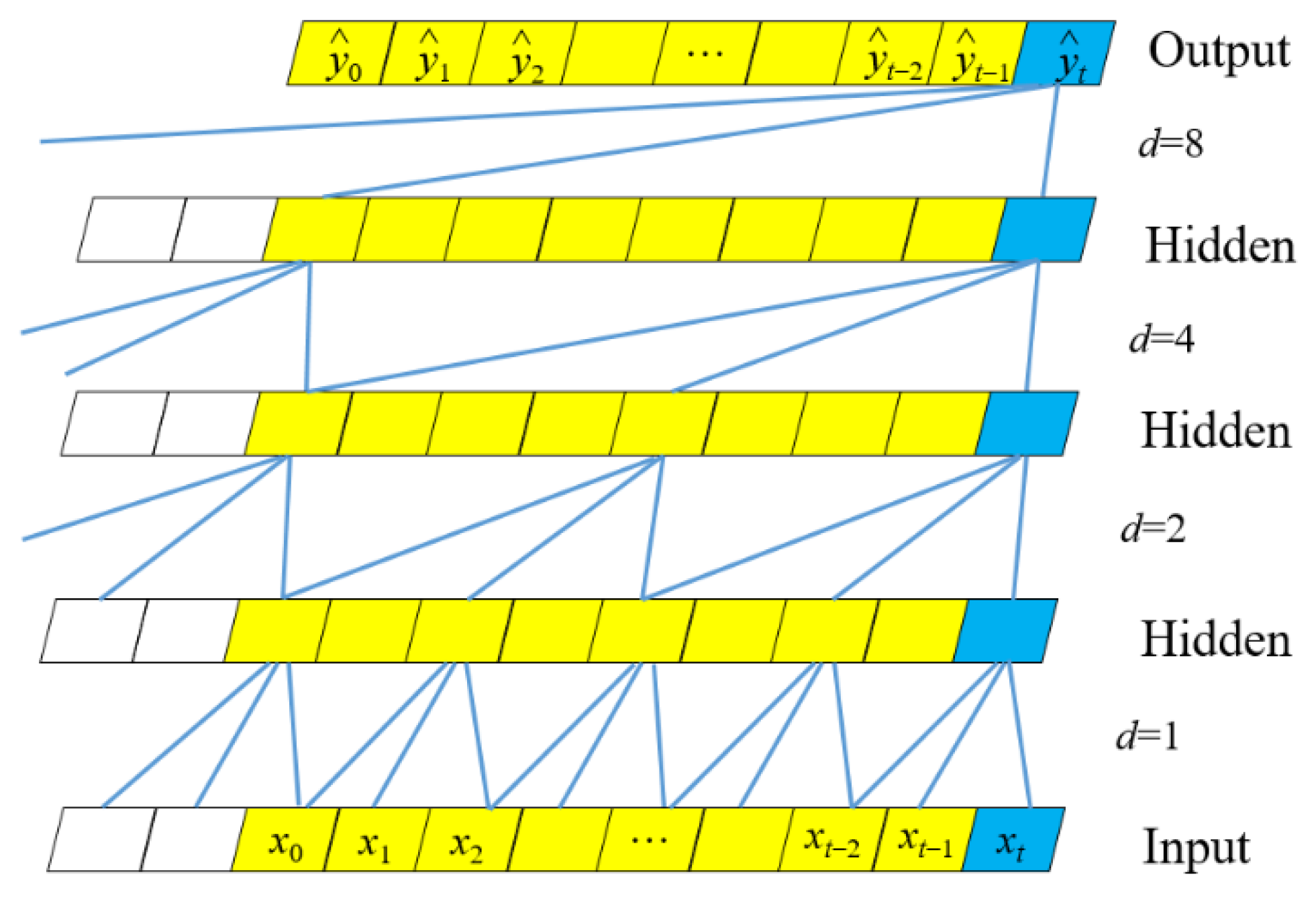
Temporal convolutional network (TCN) is an algorithm that can be used to solve time series predictions. At the same time, TCN also provides a unified method to capture spatiotemporal information hierarchically. These layers have time attributes and are used to learn global and local patterns in data. Its main features are: (1) Since each prediction can only rely on its previous prediction TCN, using causal convolution, will not have data leakage; (2) TCN combines the deep neural network and extended convolution to form a model that can save a long effective history. When the model is used for multi-dimensional data parallel input, it can maintain efficient computing efficiency [35]; (3) TCN also introduces residual network and hole convolution to construct long-term dependence, so as to effectively improve the performance of the model. The TCN model structure is shown in Figure 1. The hole coefficient at the lowest layer of the hidden layer is d = 1, which means that samples are taken at each time point during input. The next layer d = 2 means that every two time points are taken as an input, and so on. In Figure 1, the third layer is taken as an example. The convolution kernel size k = 3, and the expansion convolution calculation formula is:
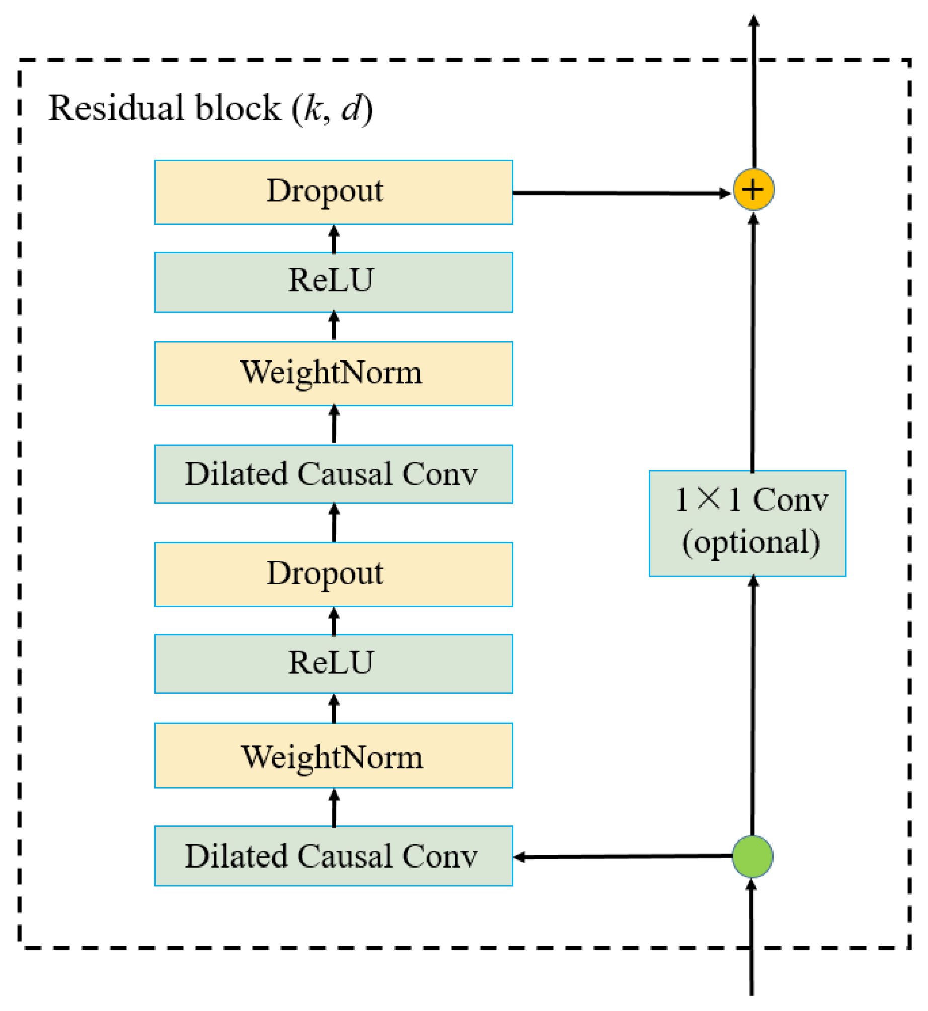
Figure 2 shows the residual network structure. Dropout means that during the neuron propagation process, the activation value of a neuron stops working with a certain probability to enhance the generalization of the model. ReLU represents the linear rectification function, which is used as the activation function of the neural network. Weight Norm means to normalize the weight value, and Dilated Causal Conv represents a dilated convolutional layer.
3.2. Long Short-Term Memory (LSTM) Model
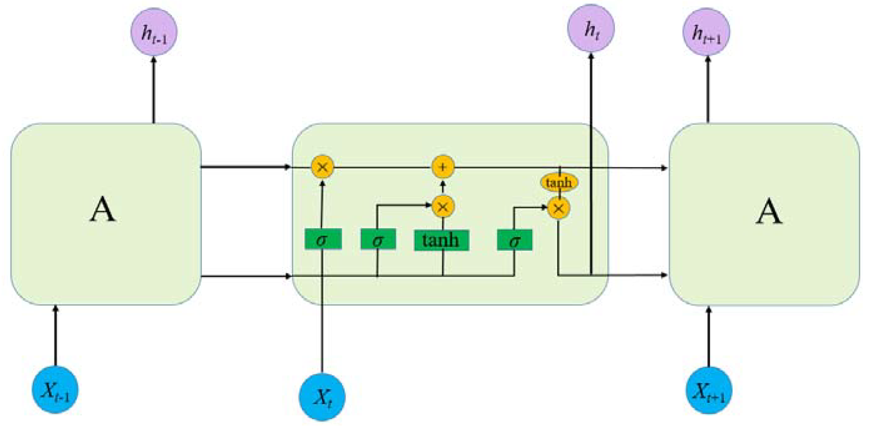
Long Short-Term Memory (LSTM) is a derivative network based on Recurrent Neural Networks (RNN). Compared with the original RNN, the gating mechanism is introduced, which can learn long-term dependencies in the input data. It can solve the problems of gradient disappearance, gradient explosion, and the inability to handle long-term dependencies caused by complex network layers [36]. Although the passenger flow of URT fluctuates greatly in the short-term, its passenger flow is still based on the changes of long-term passenger flow and the recent passenger flow level. The time correlation is significant. Therefore, the LSTM model can be used to make accurate predictions for short-term passenger flow. The model structure of LSTM is shown in Figure 3.
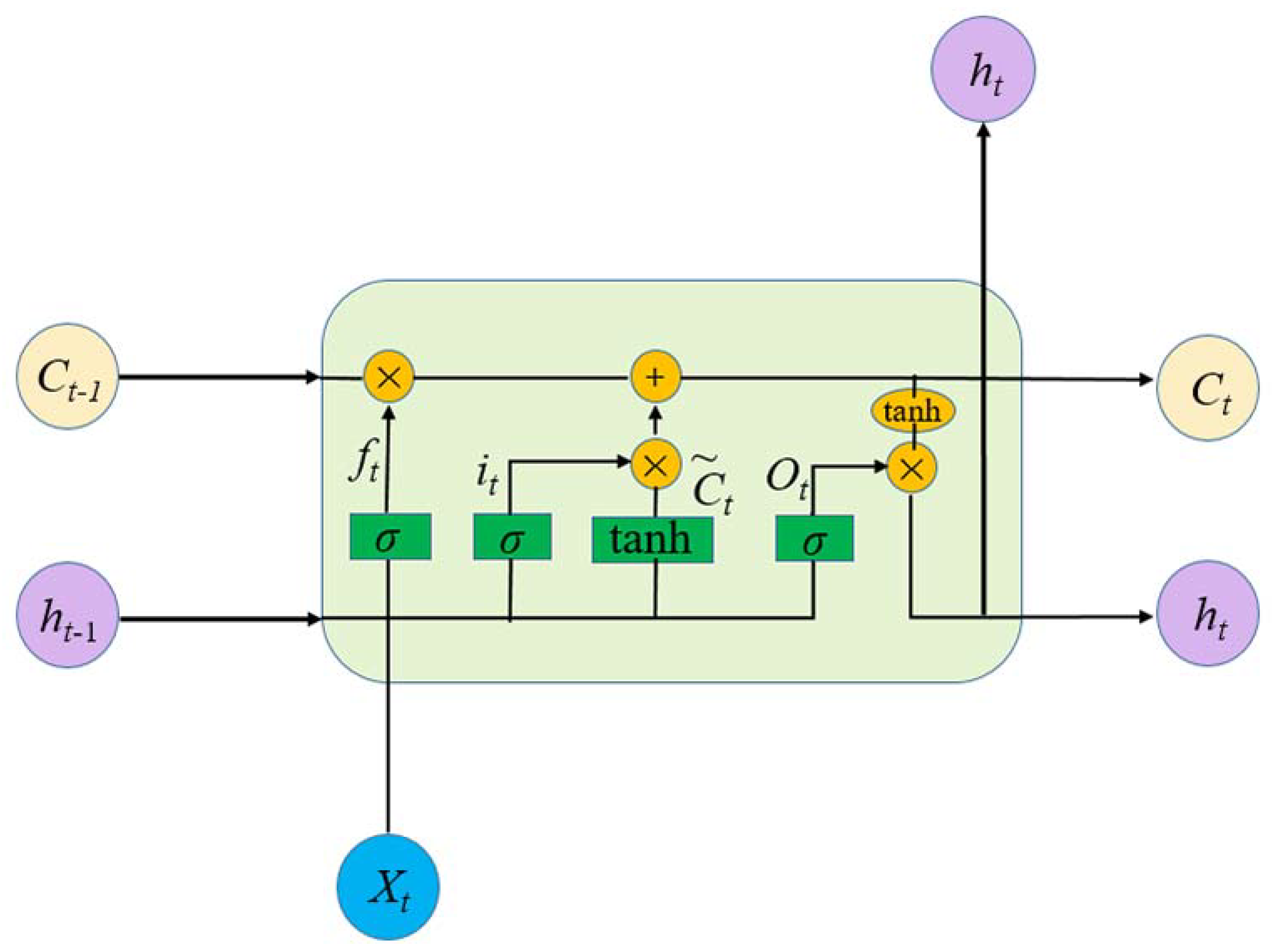
Similar to other neural networks, LSTM also has an input layer, hidden layer, and output layer. Compared with the traditional RNN model, neurons in the hidden layer can control the current memory unit through the dependency information input at the previous time and the current time. Meanwhile, the input gate, output gate, and forget gate are added to control the sequence information of memory. The structure of the memory unit in the LSTM model is shown in Figure 4. The processing flow is: Assuming that the model is at time t, the calculation completed by the memory line at time t is the passenger flow information Ct−1 at the previous moment. According to the input Xt at the current moment and the output result ht−1 at the previous moment, the forget gate ft decides to process from the previously stored information Ct−1. The forget coefficient is used to multiply the stored information Ct−1 bit by bit. The closer the vector ft is to 0, the more dependency information will be forgotten first, while the information whose value is close to 1 is retained. The forget gate calculation formula is:
where is the weight of ; is the bias condition; is the Sigmoid function, and its formula is:
After the forgetting process in the previous step, the input gate it will update the information and add it to Ct−1 according to the input information Xt at the current moment and the output information Xt−1 at the previous moment. The calculation formula of the input gate is:
where is the weight of , and is the bias condition.
After determining the value to be updated, the dependency information Ct is constructed by the tanh layer, and the state value of the memory unit will be updated by combining these two steps later. The calculation formula of new dependency information is:
where is the weight of ; is the bias condition; is a hyperbolic tangent function, and its calculation formula is:
The memory unit is updated by combining the calculated forget coefficient ft, the passenger flow dependency information Ct−1 at the previous moment, the memory coefficient it, and the new passenger flow dependency information . The calculation formula is:
The final output information is determined by the output gate according to the memory unit and the input dependency information. The calculation formula is:
where is the weight of , and is the bias condition.
3.3. TCN-LSTM Model
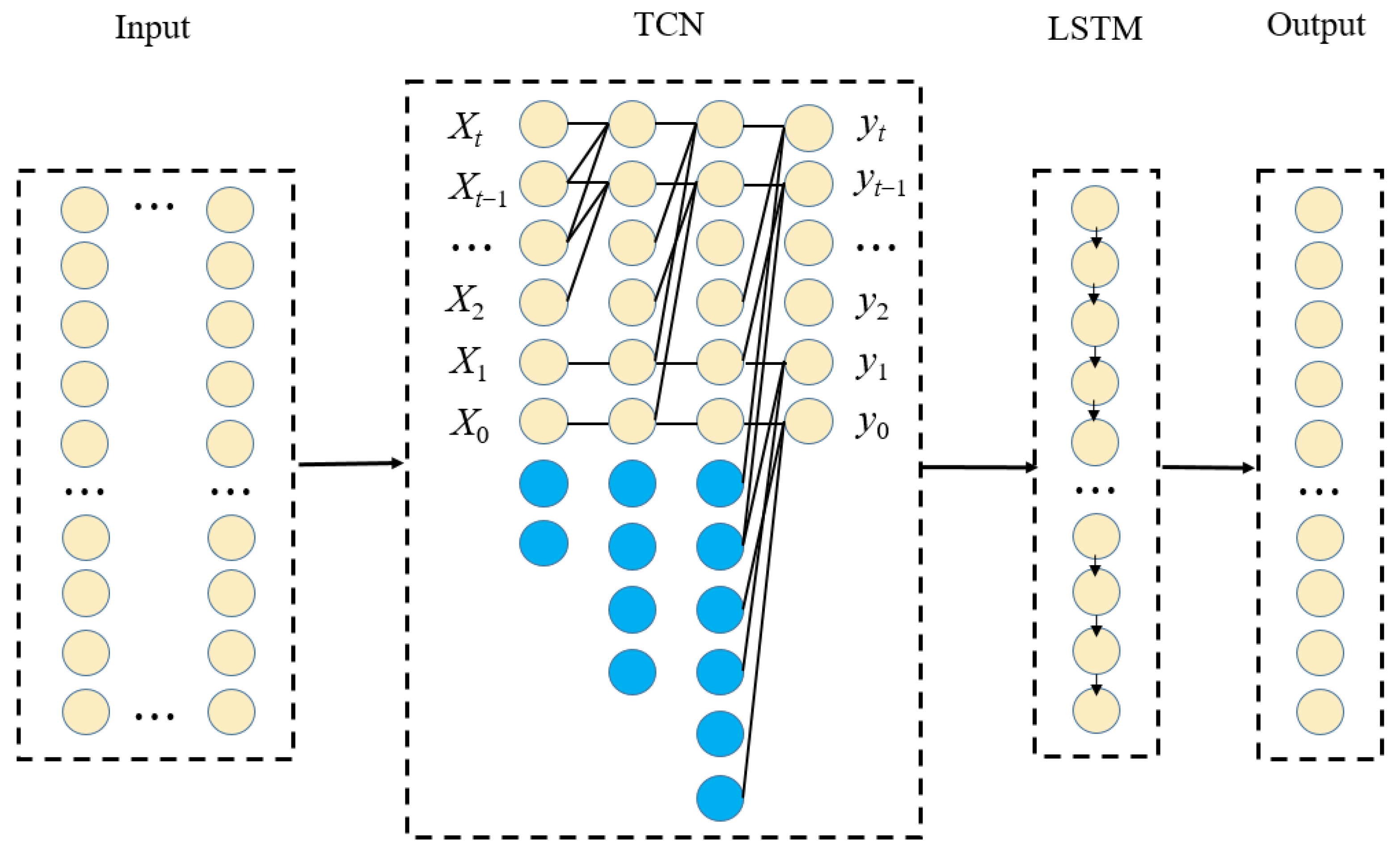
In short-term passenger flow prediction, the change of passenger flow has multiple complex characteristics, such as strong nonlinearity, weak periodicity, and correlation. A single passenger flow prediction model cannot fully capture each feature of the data. However, the combined model can alleviate this problem to a certain extent [37]. In this paper, combining the temporal convolutional network (TCN) model with the long short-term memory network (LSTM) model, a deep learning-based TCN-LSTM model is established to predict the short-term passenger flow of URT. The model structure is shown in Figure 5. The specific workflow is: first, feature extraction is performed; the parameters in each layer are normalized, and the feature data are transmitted to the TCN layer for convolution calculation. Then, the TCN layer obtains more complete sequence features through dilated convolution and causal convolution calculations, so as to extract more dilated information dependencies. Finally, the output of the TCN layer is used as the input of the LSTM network layer to further extract features while retaining the features extracted in the TCN and then merged with the features captured by the LSTM network layer. In this way, the short-term trend of passenger flow data can be captured, and the prediction results of the combined model can be obtained.
4. Analysis of Passenger Flow Characteristics and Influencing Factors of URT
In order to find out the causes of passenger flow fluctuation and external related factors of URT, it is necessary to analyze the temporal and spatial distribution characteristics and influencing factors of passenger flow before passenger flow forecasting.
4.1. Dataset Source
The dataset source is based on the swiping data of passengers entering and leaving the stations from Sigongli to Longtou Temple of Chongqing Rail Transit Line 3 in April 2021. The weather data of Chongqing during the same period is also combined. The passenger flow data comes from Chongqing Rail Transit Group. The mileage of Chongqing Rail Transit Line 3 is 67.09 km, with a total of 45 stations. Among them, there are 15 stations between Sigongli and Longtousi, including Sigongli, Lianglukou, Niujiaotuo, Guanyinqiao, Chongqing North Station South Square, and other representative business districts and interchange hub stations. The weather data comes from the National Meteorological Science Data Sharing Platform, including some basic weather indicators such as temperature, weather conditions, wind power, and air quality index. These two types of data are processed, and the passenger flow data and weather data are matched by time.
4.2. Analysis of Passenger Flow Distribution Characteristics
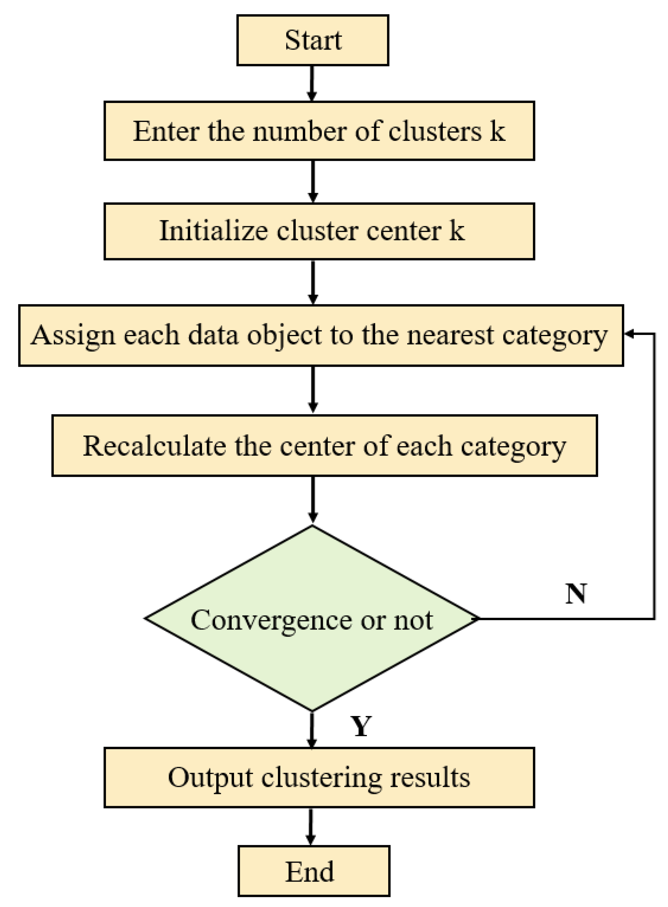
The spatial distribution characteristics of passenger flow are related to the location of stations. Based on the above daily average passenger flow data of some stations of Chongqing Rail Transit Line 3, the K-means clustering algorithm [38] is used to cluster the passenger flow of stations and determine the classification standards of passenger flow of different stations, to provide a guidance for subsequent passenger flow prediction. The K-means algorithm is an iterative clustering analysis algorithm. By updating the values of each clustering center, the samples can be clustered through this algorithm, and the samples with similar characteristics can be clustered into a class. The process is shown in Figure 6 and algorithm steps are as follows:
Step 1: For the passenger flow data set of a station, the number of categories k to be clustered is selected, and k center points are selected;
Step 2: For each sample point, the center point closest to it (find the organization) is found, and the point closest to the same center point is a class to complete a clustering;
Step 3: Determine whether the categories of the sample points before and after clustering are the same. If so, the algorithm terminates; otherwise, go to Step 4;
Step 4: For the sample points in each category, the center points of these sample points are calculated as the new center points of the class and continue Step 2.
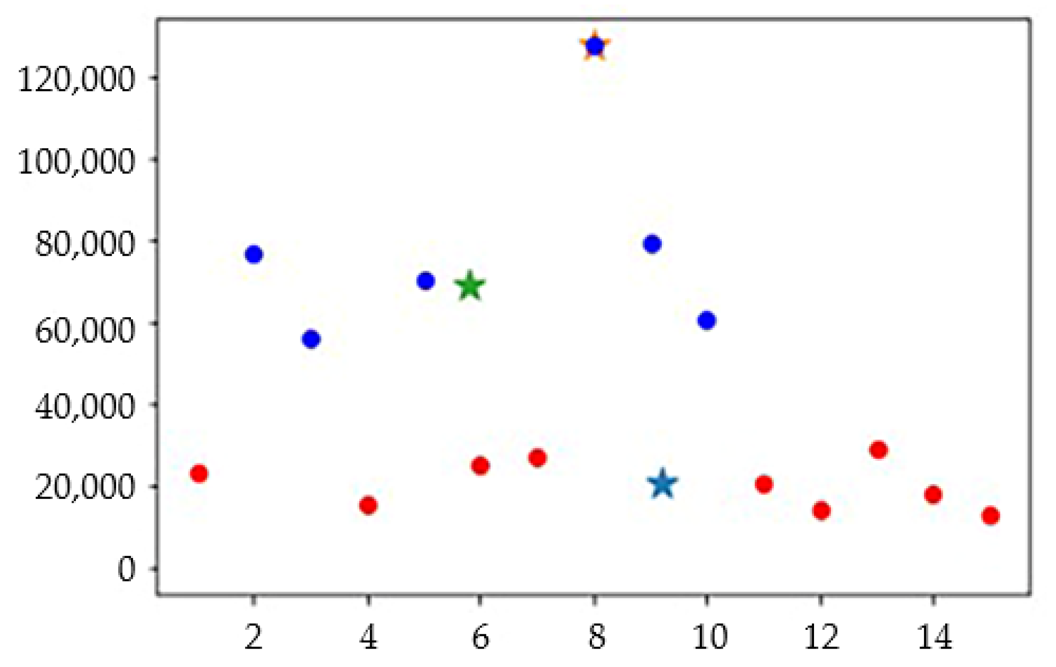
After executing the K-means algorithm on the data set, the clustering results are shown in Figure 7. It can be seen that the 15 stations are divided into three clusters, and the centroid of each cluster can better represent the characteristics of passenger flow data. The three clusters in Figure 7 are divided into three categories: high, medium, and low passenger flow, and the results are shown in Table 1. It can be seen that there is only one station with high passenger flow, which is Guanyin Bridge, with an average daily passenger flow of more than 120,000 person-times. Guanyinqiao is located in the urban tourist area of the Guanyinqiao business district in Chongqing. It is the economic center and commercial core area of Jiangbei District and is known as “the most competitive business district in China”. There are a large number of people traveling, shopping, and going to work every day. There are 5 stations with medium passenger flow, which are densely populated residential areas or business districts, or important transportation interchange hubs. The low passenger flow stations are mostly located in relatively sparsely populated areas.
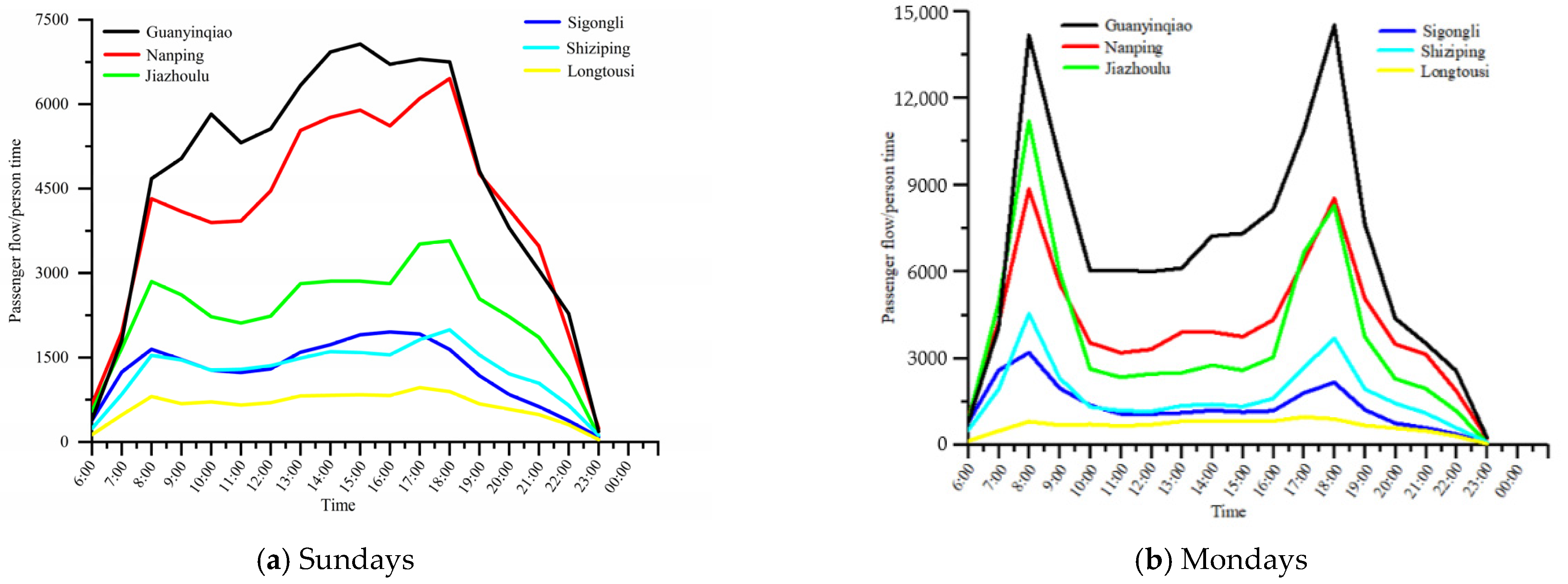
The temporal distribution characteristics of passenger flow have regular changes in the morning and evening peak due to the impact of residents’ commuting and school hours. For different stations, the morning and evening peak hours may be different. Taking the daily average station passenger flow of April 18 (Sunday) and April 19 (Monday) in 2021 as an example, the temporal distribution characteristics of high, medium (select 2 stations), and low (select 3 stations) passenger flow stations are analyzed, as shown in Figure 8.
It can be seen from Figure 8 that the passenger flow of high and medium passenger flow stations at weekends is at a high level from 8:00 to 20:00. There is a short peak around 18:00. For low passenger flow stations, there is no apparent peak. During working days, all stations have obvious morning and evening peak periods. The passenger flow has an obvious bimodal distribution, and the peak time of each station is the same. It can be seen from the analysis that the peak hours of passenger flow at different stations are 7:00–9:00 and 17:00–19:00 on weekdays, and that at the stations with high and medium passenger flow are 14:00–19:00 at weekends.
4.3. Analysis of Factors Affecting Passenger Flow
The change of URT short-term passenger flow is affected by many factors. It presents an overall law that is based on its own long-term evolution and has certain periodic and random fluctuations. Actually, not all factors have a large impact on passenger flow. Some factors such as whether it rains have a great impact on residents’ travel, which even determines the peak of the passenger flow. Some factors have little impact on passenger flow, and whether to consider them or not has no effect on the accuracy of passenger flow prediction. To achieve an accurate prediction of the short-term passenger flow of URT, it is necessary to select appropriate relevant influencing factors. The following uses the Pearson correlation coefficient analysis to determine the factors that have an impact on the passenger flow. The Pearson coefficient can measure the degree of linear correlation between two variables, so as to filter out irrelevant factors with less influence [39]. Its calculation formula is as formula (9):
where is the Pearson correlation coefficient; X is the passenger flow; Y is the corresponding influencing factors; is the covariance of X and Y; and are the standard deviation of X and Y, respectively; and are the mathematical expectations of X and Y, respectively; is the mathematical expected value after multiplying the corresponding variables of X and Y.
The Pearson correlation coefficient has a value between −1 and 1. The larger the absolute value, the stronger the correlation between the influencing factor and the passenger flow, and vice versa. The positive and negative values of represent different correlations, with greater than 0 representing positive correlation and less than 0 representing negative correlation. The Pearson correlation coefficients calculated from the data are shown in Table 2.
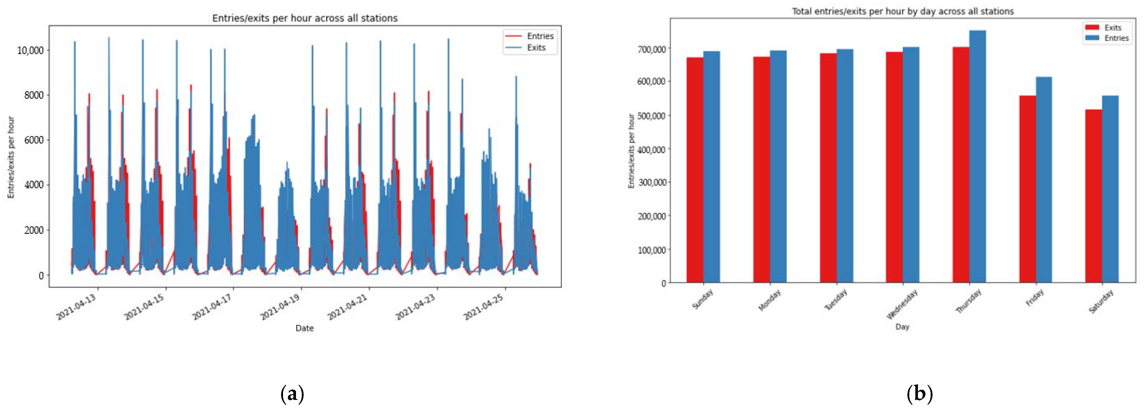
Given the influence of date attributes on passenger flow, it can be seen that the passenger flow of rail transit fluctuates depending on whether it is a working day and the passenger flow of the previous day. Daily passenger flow data and daily average passenger flow data within a week were selected for analysis, and the results are shown in Figure 9. It can be seen from Figure 9 that the peak passenger flow at weekends is significantly lower than that on working days. There is also a certain fluctuation in the peak passenger flow between two adjacent days during the week, which indicates that the date attribute has a great influence on the passenger flow. The Pearson correlation coefficient calculated according to the specific data is shown in Table 2. It can be seen that the two influencing factors of daily average passenger flow on working days and weekend holiday attributes are at a level of p < 0.01 (within the 99% confidence interval). The correlation is significant, and the correlation of the weekend holiday attribute is stronger than that of average daily passenger flow on working days.
The passenger flow of URT is time series data. The passenger flow at a certain moment is related to both the past historical passenger flow and the future passenger flow. Figure 10 is the hourly average inbound/outbound passenger flow statistics for all stations. It can be seen that there are two passenger flow peaks at 8:00 and 18:00, and the passenger flow before and after the peak is affected. Taking the time granularity of 1 h as an example, the impact of historical passenger flow on the current passenger flow in the short-term passenger flow prediction of URT was analyzed. The calculated Pearson correlation coefficient is shown in Table 2, and it can be seen that the correlation is significant (within the 99% confidence interval).
The short-term prediction of URT passenger flow in units of days also needs to consider the influence of the natural environment and weather. The weather has a great impact on residents’ travel, especially those residents who go out shopping and playing, who flexibly choose travel methods and times according to weather conditions. This paper mainly analyzes the influence of weather conditions such as temperature, weather conditions, wind power, and air quality index on passenger flow. The calculated Pearson correlation coefficients are shown in Table 2. According to Table 2, except for the wind factor, the other influencing factors are all within the 99% confidence interval.
According to the above analysis, it can be found that there are several factors affecting the URT passenger flow. In this paper, six factors except the wind factor are used as the parameter indicators to analyze and predict the short-term passenger flow. Details are shown in Table 3.
5. Application Analysis of Passenger Flow Prediction
Taking the passenger flow data of Chongqing Rail Transit Line 3 in April 2021 as an example, based on the above TCN-LSTM model, the first 80% of the data is taken as the training sample and the last 20% as the test sample. The short-term passenger flow of rail traffic is predicted in a short time to verify the prediction accuracy and validity of the model.
5.1. Data Processing
The method described in Section 4.3 is used to preprocess the raw data and encode date attributes and weather factors. The time period 6:00–23:00 is selected as the target time period for passenger flow research, and 1 h as the time slice, i.e., passenger flow is counted every 1 h. The experimental running environment of this paper is python3.10, and the short-term passenger flow prediction model is built by the third-party libraries of Scikit-learn, Keras, and TensorFlow in python.
The above data is input into the TCN-LSTM model, and the convolution kernel size is k = 3. The upper and lower limits of the hidden layers of the TCN network are set to 8 and 64, respectively, and that of the LSTM network is set to 64 and 128, respectively. The training times are 100, and the learning rate is 0.01. Other parameters remain unchanged.
5.2. Results and Analysis of Short-Term Passenger Flow Prediction
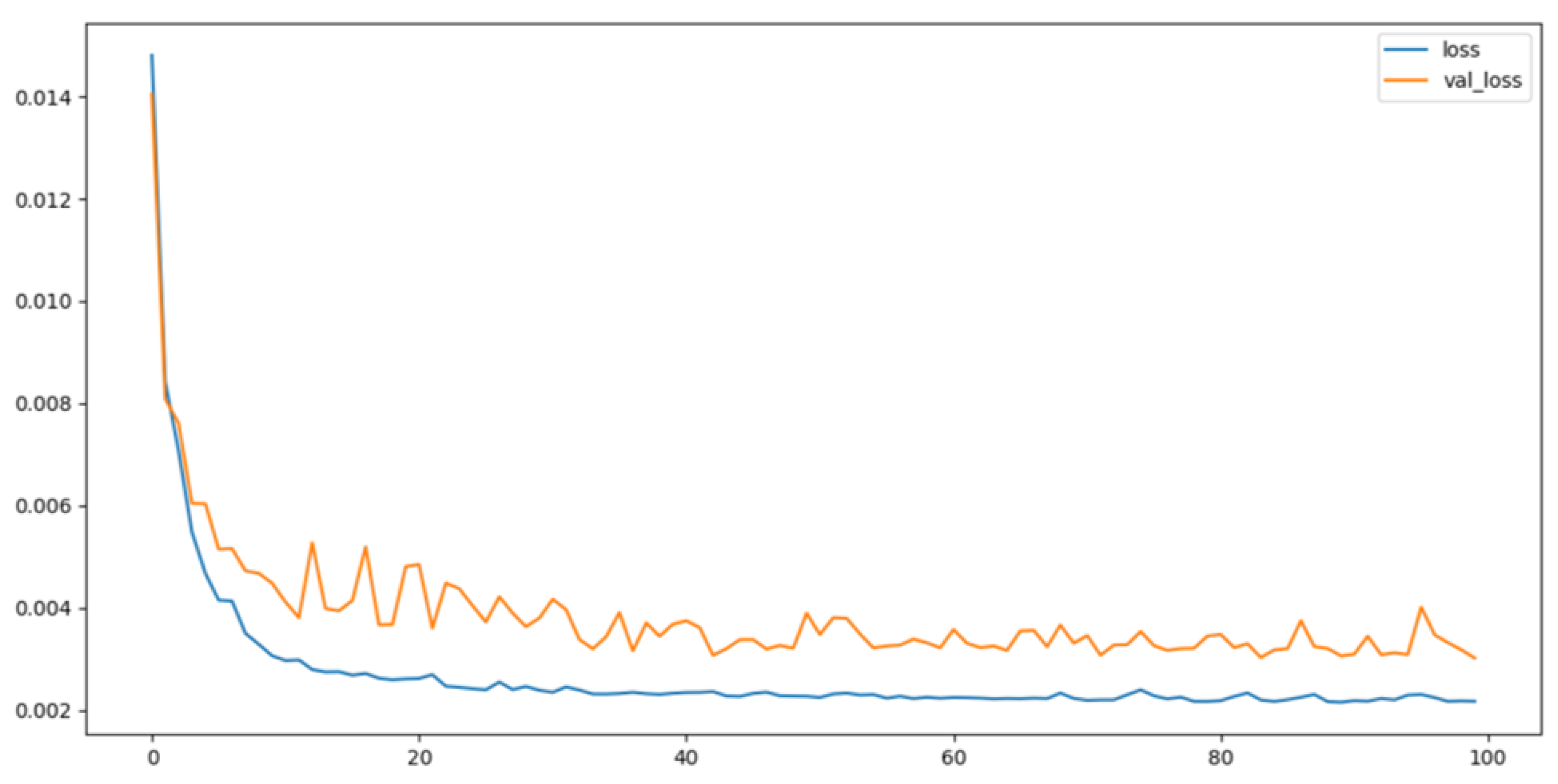
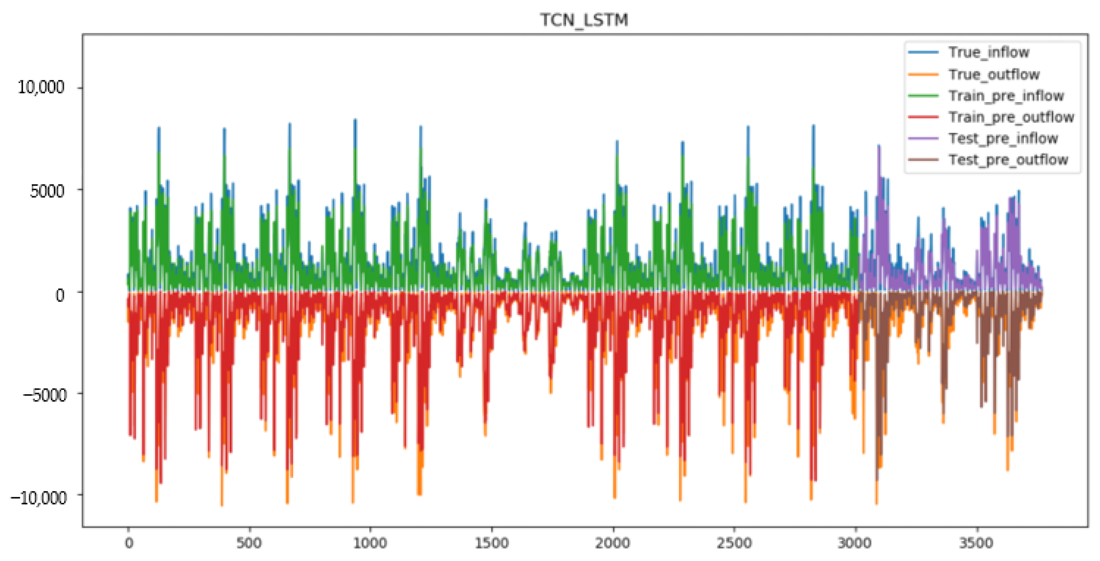
Using the TCN-LSTM combination model to analyze and predict the above passenger flow data, the loss value curves of the training set and test set are shown in Figure 11. It can be seen that both curves drop to a stable value, indicating that the trained network behaves normally. The total passenger flow prediction results are shown in Figure 12. It can be seen that the TCN-LSTM model can approximately capture the changing characteristics of the real URT passenger flow to a certain extent and can reflect the law of short-term traffic passenger flow changing with time. At the same time, to compare and verify the accuracy of the TCN-LSTM model, this paper also established a single LSTM model to predict the passenger flow, as shown in Figure 13.
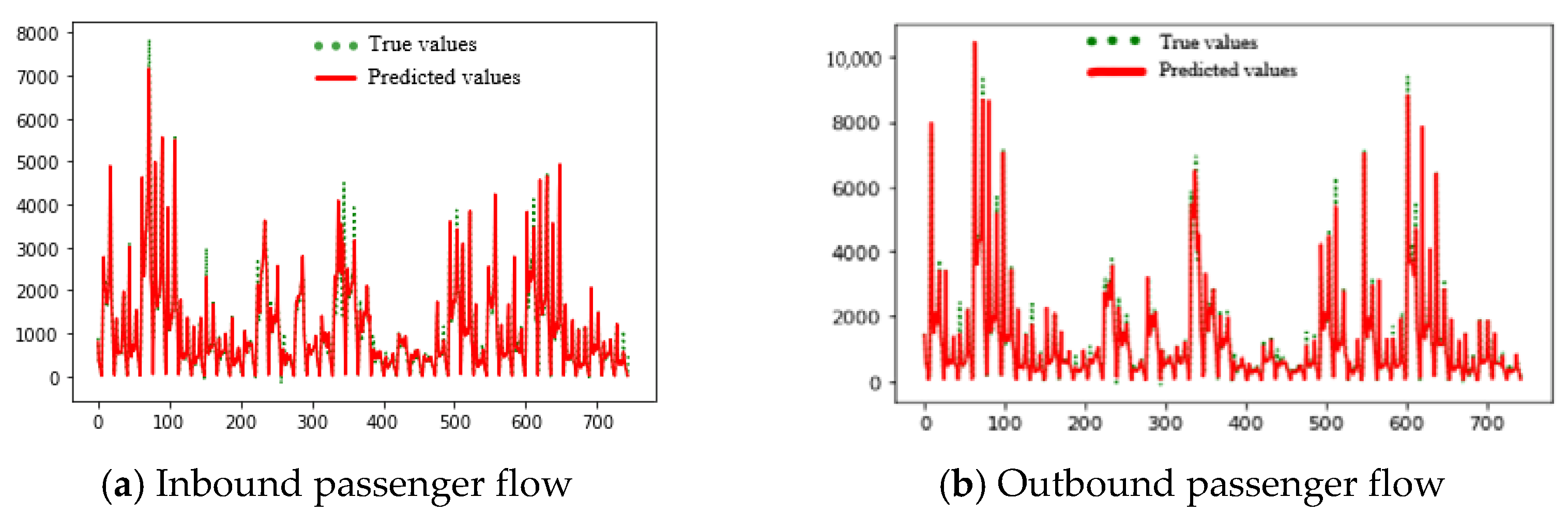
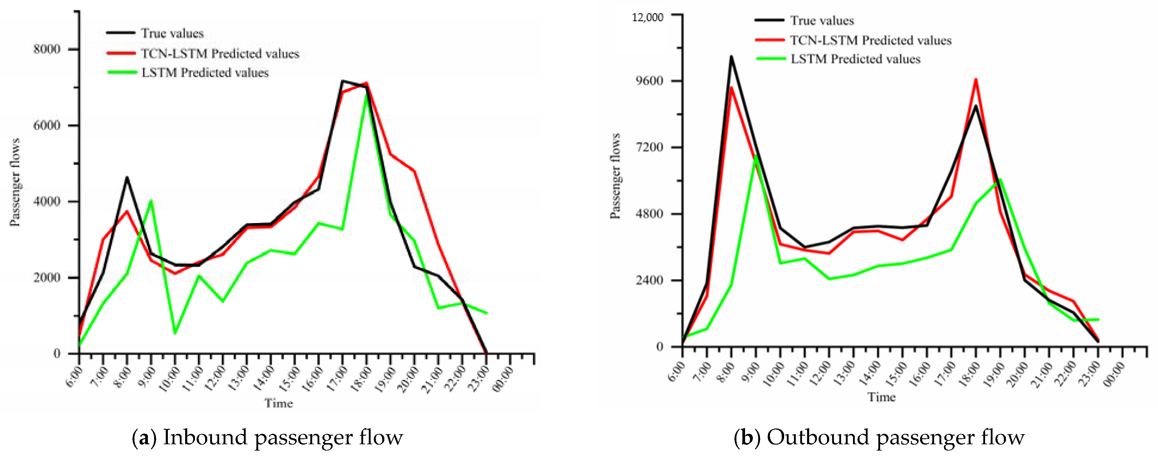
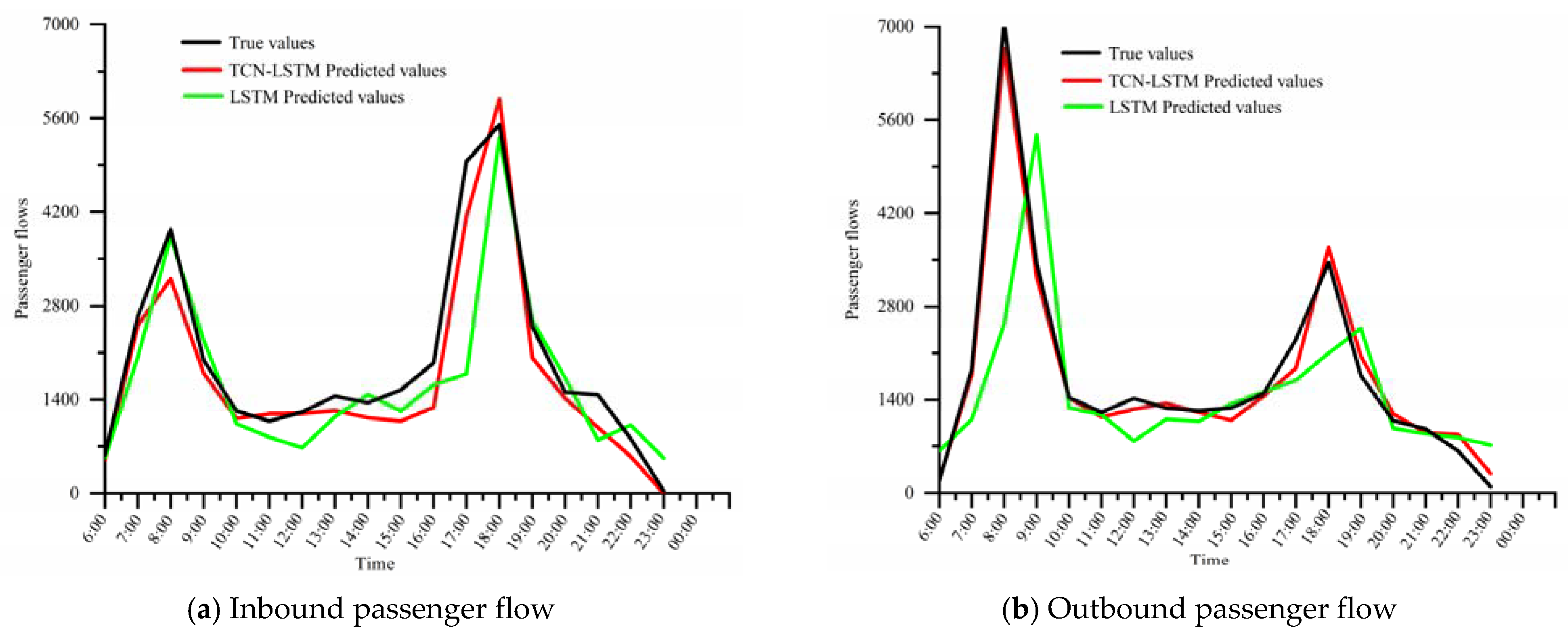
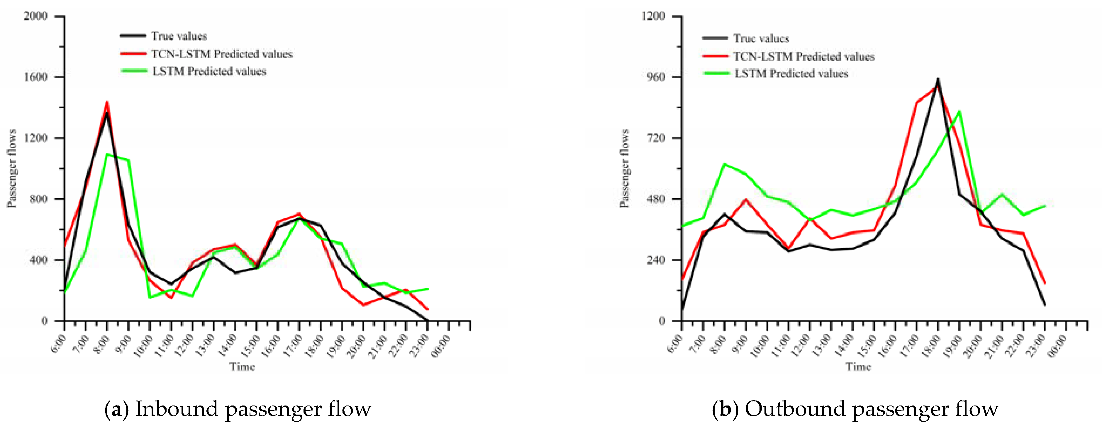
To more intuitively demonstrate the ability of the TCN-LSTM model to capture the passenger flow characteristics, the prediction of inbound/outbound passenger flow in different time segments of rail transit was analyzed for specific high, medium, and low passenger flow stations. The prediction results of the single LSTM model were compared as shown in Figure 14, Figure 15 and Figure 16. It can be seen that the prediction performance of the LSTM single model is poor, and the prediction error of the peak passenger flow is large. The prediction results of the two models show that the TCN-LSTM model is superior to the single LSTM model both in the short-term passenger flow prediction and data generalization of URT.
5.3. Model Comparison Evaluation
To better compare the difference in prediction effect between the combined model and the single model, two common evaluation indicators, root mean square error (RMSE) and mean absolute percentage error (MAPE), were used to quantify the performance of the model according to different categories of stations. Its calculation formula is:
where N is the total samples; is the actual value of passenger flow; and is the predicted value of passenger flow. RMSE and MAPE can represent the gap between the predicted value and real value. Thereby the performance of the model only needs to compare the RMSE and MAPE values of the prediction results. The smaller the value of the two evaluation indicators, the better the prediction result of the model.
Table 4 shows the RMSE and MAPE values obtained by using the combined model and the single model to predict the passenger flow of different stations. It can be seen that the prediction results of the TCN-LSTM combined model are better than the LSTM single model for high, medium, and low passenger flow stations. However, for the combined model, the prediction accuracy of the low passenger flow is the lowest, and the higher the passenger flow, the better the prediction accuracy of the combined model.
6. Discussion
From the above example prediction results, the prediction accuracy of TCN-LSTM combined deep learning model constructed in this paper is much higher than that of LSTM single model. As can be seen from Table 4, the RMSE values of the prediction results of the TCN-LSTM combined deep learning model constructed in this paper has decreased by 66%, 20%, and 17% respectively in high (Guanyinqiao), medium (Jiazhoulu), and low (Longtousi) passenger flow stations compared with the LSTM single model. MAPE values decreased by 69%, 26%, and 18% respectively in high (Guanyinqiao), medium (Jiazhoulu), and low (Longtousi) passenger flow stations. On the one hand, it shows that the prediction model proposed in this paper has good simulation accuracy. On the other hand, it was found that the decrease of the predicted indicator values will increase with the increase of passenger flow.
When combined with the passenger flow prediction curves between different stations, it was found that in medium and high passenger flow stations, the TCN-LSTM model has higher coupling and lower oscillation in the prediction of the overall trend, and the overall prediction accuracy is more accurate. In low passenger flow stations, the prediction trend of TCN-LSTM model fluctuates greatly, and the variation range of accuracy shows an unstable trendy, which is consistent with the results fed back by RMSE values and MAPE values. This may be related to the sample point data of high passenger flow stations. The sample data base of high passenger flow stations is large, which is also greatly affected by external factors, and the passenger flow presents a double peak distribution. The TCN-LSTM combined forecasting model proposed in this paper not only couples multi-source external factors, but also has a better ability to capture the peak passenger flow than a single LSTM model, which leads to a large difference in the forecasting performance in high passenger flow stations. However, the sample data base of low passenger flow stations is small, which is less affected by external factors, and the passenger flow shows a single peak distribution, which shows little difference in performance between the two models.
In addition, the prediction results of the LSTM model show that the fitting degree of the LSTM single model is not good. The analysis reason is that when the passenger flow and passenger flow characteristic dimensions are increased, the structure of the LSTM model limits the calculation efficiency and accuracy. It also shows that with the increase of the complexity of the actual situation, the prediction model with a simple mathematical model or machine learning algorithm as the main support is difficult to meet practical needs.
According to the above discussion, the TCN-LSTM combined prediction model proposed in this paper has the following advantages. (1) Compared with a single LSTM model that can only capture the temporal characteristics of passenger flow data, a TCN-LSTM model integrates temporal and spatial prediction, the accuracy and stability of passenger flow prediction have been greatly improved. (2) The TCN-LSTM model is closer to the real prediction situation because it couples external factors such as date attributes, weather conditions, and air quality. (3) The TCN-LSTM model has a stronger ability to capture the peak passenger flow, and the peak passenger flow of rail transit has more reference value for the reasonable planning of passenger travel time and the operation and management of line train numbers.
7. Conclusions
Aiming at the problem of short-term passenger flow prediction in URT, this paper proposes a TCN-LSTM prediction model considering multiple factors influencing passenger flow. Based on the passenger flow data of some stations of Chongqing Rail Transit Line 3, external factors such as date attributes, weather conditions, and air quality are coupled into the prediction model. The short-term passenger flow predictions of the combined model and the single model are carried out respectively. The results show that:
(1) After analyzing the temporal and spatial distribution characteristics of passenger flow, the correlation analysis of passenger flow influencing factors can provide a good data set for the follow-up short-term passenger flow prediction model of urban rail transit to accurately predict the short-term passenger flow.
(2) The Long Short-Term Memory (LSTM) network model can fully mine and effectively use the relationship between historical passenger flow data and can better predict the passenger flow trend of different passenger flow types of stations.
(3) The TCN-LSTM combined model can make up for the deficiency of the LSTM single model in the actual passenger flow forecast, and its RMSE and MAPE values are significantly reduced. Through the comparison of the two forecast results, it was found that the TCN-LSTM combined model performs better than the LSTM single model in the peak, flat peak, and all-day stages of passenger flow forecast, and can more accurately predict changes in short-term passenger flow.
(4) The short-term passenger flow forecast of urban rail transit carried out in this paper can provide some technical support for rail transit line planning and vehicle operation scheduling.
This combined neural network model based on deep learning still has room for optimization in parameter setting and model training in the short-term passenger flow forecast of urban rail transit. In the future, the model can be optimized to achieve a better forecasting effect and can be extended to the short-term passenger flow forecast of different cities and scenarios.
Author Contributions
Conceptualization, Z.Y.; Formal analysis, G.Y.; Supervision, Z.D.; Writing—original draft, Z.H. All authors have read and agreed to the published version of the manuscript.
Funding
This work was supported by the National Natural Science Foundation of China (Grant No. 52072054); the Science and Technology Research Program of Chongqing Municipal Education Commission (Grant No. KJQN202100729); the Natural Science Foundation of Chongqing, China, (Grant No. cstc2021jcyjmsxmX0534); Chongqing Smart City and Sustainable Development Academy Application Form for Tech-Inno Fund Project (Grant No. 20210601); and the Opening Fund of Urban Rail Transit Vehicle System Integration and Control Laboratory in Chongqing (Grant No. CKLURTSIC-KFKT-201810). The authors are deeply grateful for this support. The comments of the anonymous reviewers have improved the quality of this paper and are also gratefully acknowledged.
Institutional Review Board Statement
Not applicable.
Informed Consent Statement
Not applicable.
Data Availability Statement
Data is contained within the present article.
Conflicts of Interest
The authors declare no conflict of interest.
Abbreviations
| URT | Urban rail transit |
| LSTM | Long Short-Term Memory |
| TCN | Temporal Convolutional Network |
| ARIMA | Autoregressive Integrated Moving Average model |
| LR | Logistic Regression |
| GM | Grey Model |
| SVM | Support Vector Machine |
| RNN | Recurrent Neural Network |
| ARMA | Autoregressive Moving Average model |
| PSO | Particle Swarm Optimization |
| CNN | Convolutional Neural Network |
| NAR | Nonlinear regression |
| SARIMA | Seasonal autoregressive integrated moving average |
| GRU | Gated recurrent unit |
| GCN | Graph convolutional network |
| RMSE | Root mean square error |
| MAPE | Mean absolute percent error |
References
- China Association of Metros. 2020 Statistical and Analysis Report for Urban Rail Transit. Tunn. Constr. 2021, 41, 691. [Google Scholar]
- Liang, S.; Ma, M.; He, S.; Zhang, H. Short-Term Passenger Flow Prediction in Urban Public Transport: Kalman Filtering Combined K-Nearest Neighbor Approach. IEEE Access 2019, 7, 120937–120949. [Google Scholar] [CrossRef]
- Liu, S.Y.; Liu, S.; Tian, Y.; Sun, Q.L.; Tang, Y.Y. Research on Forecast of Rail Traffic Flow Based on ARIMA Model. J. Phys. Conf. Ser. 2021, 1792, 012065. [Google Scholar] [CrossRef]
- Smith, B.L.; Williams, B.M.; Oswald, R.K. Comparison of parametric and nonparametric models for traffic flow forecasting. Transp. Res. Part C Emerg. Technol. 2002, 10, 303–321. [Google Scholar] [CrossRef]
- Yang, J.; Hou, Z.S. A grey Markov based on large passenger flow real-time prediction model. J. Beijing Jiaotong Univ. 2013, 37, 119–123, 128. [Google Scholar]
- Zhang, Y.; Liu, Y. Traffic forecasting using least squares support vector machines. Transportmetrica 2009, 5, 193–213. [Google Scholar] [CrossRef]
- Wei, Y.; Chen, M.-C. Forecasting the short-term metro passenger flow with empirical mode decomposition and neural networks. Transp. Res. Part C Emerg. Technol. 2012, 21, 148–162. [Google Scholar] [CrossRef]
- Tsai, T.-H.; Lee, C.-K.; Wei, C.-H. Neural network based temporal feature models for short-term railway passenger demand forecasting. Expert Syst. Appl. 2009, 36, 3728–3736. [Google Scholar] [CrossRef]
- Long, X.Q.; Li, J.; Chen, Y.R. Metro short-term traffic flow prediction with deep learning. Control. Decis. 2019, 34, 1589–1600. [Google Scholar]
- Polson, N.G.; Sokolov, V.O. Deep learning for short-term traffic flow prediction. Transp. Res. Part C Emerg. Technol. 2017, 79, 1–17. [Google Scholar] [CrossRef] [Green Version]
- Lv, Y.; Duan, Y.; Kang, W.; Li, Z.; Wang, F.-Y. Traffic Flow Prediction With Big Data: A Deep Learning Approach. IEEE Trans. Intell. Transp. Syst. 2015, 16, 865–873. [Google Scholar] [CrossRef]
- Zhao, Z.; Chen, W.; Wu, X.; Chen, P.C.Y.; Liu, J. LSTM network: A deep learning approach for short-term traffic forecast. IET Intell. Transp. Syst. 2017, 11, 68–75. [Google Scholar] [CrossRef] [Green Version]
- Chu, J.; Su, Y.W.; Wang, L. Scene classification with adaptive learning rate and sample training mode. Pattern Recognit. Artif. Intell. 2018, 31, 625–633. [Google Scholar]
- Lei, B.; Zhang, Y.; Hao, Y.R.; Jing, L.Z. Research progress on short-term passenger flow forecast model of urban rail transit. J. Chang’an Univ. (Nat. Sci. Ed.) 2022, 42, 79–96. [Google Scholar]
- Ma, X.; Yunpeng, W.; Wang, Y.; Wang, Y. Large-Scale Transportation Network Congestion Evolution Prediction Using Deep Learning Theory. PLoS ONE 2015, 10, e0119044. [Google Scholar] [CrossRef] [PubMed]
- Ma, X.; Tao, Z.; Wang, Y.; Yu, H.; Wang, Y. Long short-term memory neural network for traffic speed prediction using remote microwave sensor data. Transp. Res. Part C Emerg. Technol. 2015, 54, 187–197. [Google Scholar] [CrossRef]
- Zhang, J.; Chen, F.; Shen, Q. Cluster-Based LSTM Network for Short-Term Passenger Flow Forecasting in Urban Rail Transit. IEEE Access 2019, 7, 147653–147671. [Google Scholar] [CrossRef]
- Zhang, J.; Chen, F.; Cui, Z.; Guo, Y.; Zhu, Y. Deep Learning Architecture for Short-Term Passenger Flow Forecasting in Urban Rail Transit. IEEE Trans. Intell. Transp. Syst. 2020, 22, 7004–7014. [Google Scholar] [CrossRef]
- Shao, H.; Soong, B.H. Traffic flow prediction with Long Short-Term Memory Networks (LSTMs). In Proceedings of the 2016 IEEE Region 10 Conference, Singapore, 22–25 November 2016; pp. 2986–2989. [Google Scholar]
- Shitan, M.; Karmokar, P.K.; Lerd, N.Y. Time Series Modeling And Forecasting of Ampang Line Passenger Ridership In Ma-laysia. Pak. J. Stat. 2014, 30, 385–396. [Google Scholar]
- Cvetek, D.; Mustra, M.; Jelusic, N.; Abramovic, B. Traffic Flow Forecasting at Micro-Locations in Urban Network using Bluetooth Detector. In Proceedings of the 2020 International Symposium ELMAR, Zadar, Croatia, 14–15 September 2020; pp. 57–60. [Google Scholar] [CrossRef]
- Kumar, S.V.; Vanajakshi, L. Short-term traffic flow prediction using seasonal ARIMA model with limited input data. Eur. Transp. Res. Rev. 2015, 7, 21. [Google Scholar] [CrossRef] [Green Version]
- Ye, H.; Hao, Y.; Zhu, H. ‘N-Day’ Average Volume Based Analysis and Forecasting for Daily Passenger Flow of Shanghai URT. In Proceedings of the 2nd International Conference on Transportation Engineering, Chengdu, China, 25–27 July 2009; pp. 4080–4085. [Google Scholar] [CrossRef]
- Haworth, J.; Shawe-Taylor, J.; Cheng, T.; Wang, J. Local online kernel ridge regression for forecasting of urban travel times. Transp. Res. Part C Emerg. Technol. 2014, 46, 151–178. [Google Scholar] [CrossRef] [Green Version]
- Sun, Y.; Song, X.Y.; Jin, L.T.; Liu, T. Railway Passenger Flow Forecast Based on Arma-Lstm Combined Model. Computer Ap-plications and Software. Comput. Appl. Softw. 2021, 38, 262–267, 273. [Google Scholar]
- Teng, J.; Li, J.Y. Short-Term Forecast Method for Intercity Railway Passenger Flow Considering Date Attributes and Weather Factors. China Railw. Sci. 2020, 41, 136–144. [Google Scholar]
- Wu, Y.; Tan, H. Short-term traffic flow forecasting with spatial-temporal correlation in a hybrid deep learning framework. arXiv 2016, arXiv:1612.01022. [Google Scholar] [CrossRef]
- Yang, X.; Xue, Q.; Yang, X.; Yin, H.; Qu, Y.; Li, X.; Wu, J. A novel prediction model for the inbound passenger flow of urban rail transit. Inf. Sci. 2021, 566, 347–363. [Google Scholar] [CrossRef]
- Li, W.; Sui, L.; Zhou, M.; Dong, H. Short-term passenger flow forecast for urban rail transit based on multi-source data. EURASIP J. Wirel. Commun. Netw. 2021, 2021, 9. [Google Scholar] [CrossRef]
- Do, L.N.; Vu, H.L.; Vo, B.Q.; Liu, Z.; Phung, D. An effective spatial-temporal attention based neural network for traffic flow prediction. Transp. Res. Part C Emerg. Technol. 2019, 108, 12–28. [Google Scholar] [CrossRef]
- Wu, Y.; Tan, H.; Qin, L.; Ran, B.; Jiang, Z. A hybrid deep learning based traffic flow prediction method and its understanding. Transp. Res. Part C Emerg. Technol. 2018, 90, 166–180. [Google Scholar] [CrossRef]
- Defferrard, M.; Bresson, X.; Vandergheynst, P. Convolutional Neural Networks on Graphs with Fast Localized Spectral Filtering. Adv. Neural Inf. Process. Syst. 2016, 29. [Google Scholar] [CrossRef]
- Zhao, L.; Song, Y.; Zhang, C.; Liu, Y.; Wang, P.; Lin, T.; Deng, M.; Li, H. T-GCN: A Temporal Graph Convolutional Network for Traffic Prediction. IEEE Trans. Intell. Transp. Syst. 2020, 21, 3848–3858. [Google Scholar] [CrossRef] [Green Version]
- Hao, S.; Lee, D.-H.; Zhao, D. Sequence to sequence learning with attention mechanism for short-term passenger flow prediction in large-scale metro system. Transp. Res. Part C Emerg. Technol. 2019, 107, 287–300. [Google Scholar] [CrossRef]
- Hewage, P.; Behera, A.; Trovati, M.; Pereira, E.; Ghahremani, M.; Palmieri, F.; Liu, Y. Temporal convolutional neural (TCN) network for an effective weather forecasting using time-series data from the local weather station. Soft Comput. 2020, 24, 16453–16482. [Google Scholar] [CrossRef] [Green Version]
- Liu, Q.H.; Zhang, R.; Wang, Y.; Yan, H.; Hong, M. Daily Prediction of the Arctic Sea Ice Concentration Using Reanalysis Data Based on a Convolutional LSTM Network. J. Mar. Sci. Eng. 2021, 9, 330. [Google Scholar] [CrossRef]
- Li, W.-Q.; Chang, L. A combination model with variable weight optimization for short-term electrical load forecasting. Energy 2018, 164, 575–593. [Google Scholar] [CrossRef]
- Kanungo, T.; Mount, D.M.; Netanyahu, N.S.; Piatko, C.D.; Silverman, R.; Wu, A.Y. An efficient k-means clustering algorithm: Analysis and implementation. IEEE Trans. Pattern Anal. Mach. Intell. 2002, 24, 881–892. [Google Scholar] [CrossRef]
- Cai, J.; Xu, K.; Zhu, Y.; Hu, F.; Li, L. Prediction and analysis of net ecosystem carbon exchange based on gradient boosting regression and random forest. Appl. Energy 2020, 262, 114566. [Google Scholar] [CrossRef]
Figure 1.
Schematic diagram of TCN model structure.

Figure 2.
Residual network structure.

Figure 3.
Structural diagram of LSTM model.

Figure 4.
Structure of LSTM memory unit.

Figure 5.
Structure diagram of TCN-LSTM model.

Figure 6.
K-means algorithm execution process.

Figure 7.
Clustering results after executing K-means algorithm. In the figure, red circles represent low passenger flow stations, blue circles represent medium and high passenger flow stations, and asterisks represent clustering centers.
Figure 7.
Clustering results after executing K-means algorithm. In the figure, red circles represent low passenger flow stations, blue circles represent medium and high passenger flow stations, and asterisks represent clustering centers.

Figure 8.
Distribution characteristics of passenger flow on weekdays and non-weekdays at different stations over time.
Figure 8.
Distribution characteristics of passenger flow on weekdays and non-weekdays at different stations over time.

Figure 9.
Influence of date attribute on URT passenger flow. (a) Daily inbound/outbound passenger flow statistics; (b) Statistics of daily average inbound/outbound passenger flow within a week.
Figure 9.
Influence of date attribute on URT passenger flow. (a) Daily inbound/outbound passenger flow statistics; (b) Statistics of daily average inbound/outbound passenger flow within a week.

Figure 10.
Hourly average inbound/outbound passenger flow statistics.

Figure 11.
Structural diagram of TCN-LSTM model.

Figure 12.
Prediction results of short-term passenger flow based on TCN-LSTM model.

Figure 13.
Prediction results of short-term passenger flow based on LSTM model.

Figure 14.
Prediction results of passenger flow at Guanyinqiao (high passenger flow).

Figure 15.
Prediction results of passenger flow at Jiazhoulu (medium passenger flow).

Figure 16.
Prediction results of passenger flow at Longtousi (Low passenger flow).


Table 1.
Cluster analysis results of some stations of Chongqing Rail Transit Line 3.
| Categories | Stations | Name of Stations | Average Daily Passenger Flow/Person-Time |
|---|---|---|---|
| High passenger flow | 1 | Guanyinqiao | ≥80,000 |
| Medium passenger flow | 5 | Nanping, Gongmao, Lianglukou, Hongqihegou, Jiazhoulu | 30,000–80,000 |
| Low passenger flow | 9 | Sigongli, Tongyuanju, Niujiaotuo, Huaxinjie, Zhengjiayuanzi, Tangjia yuanzi, Shiziping, Chongqing North Station South Square, Longtousi | <30,000 |
Table 2.
Pearson correlation coefficient of factors affecting passenger flow.
| Relevant Influencing Factors | Pearson Correlation Coefficient | Significance (Two-Tailed) |
|---|---|---|
| Average daily passenger flow on weekdays | 0.710 | 0.000 |
| Weekend holiday properties | −0.915 | 0.000 |
| Passenger flow per hour | −0.213 | 0.008 |
| Temperature | −0.747 | 0.000 |
| Weather conditions | −0.354 | 0.003 |
| Wind power | −0.023 | 0.290 |
| Air quality index | −0.235 | 0.005 |
Table 3.
Influencing parameters of passenger flow analysis and prediction.
| Variables | Illustrations | Variables | Illustrations |
|---|---|---|---|
| Y1 | Average daily passenger flow/person time on working days | Y4 | Temperature/°C |
| Y2 | Weekend holiday attribute (0 means working day, and 1 means weekend) | Y5 | Weather conditions (1 means sunny; 2 means cloudy; 3 means cloudy, and 4 means rainy) |
| Y3 | Passenger flow per hour/person time | Y6 | Air quality index/dimensionless relative value |
Table 4.
Comparison evaluation results of model prediction.
| Stations | Prediction Model | RMSE | MAPE/% |
|---|---|---|---|
| Guanyinqiao | TCN-LSTM model | 24.70 | 8.56 |
| Single LSTM model | 72.58 | 27.50 | |
| Jiazhoulu | TCN-LSTM model | 36.37 | 11.34 |
| Single LSTM model | 45.64 | 15.32 | |
| Longtousi | TCN-LSTM model | 48.45 | 16.58 |
| Single LSTM model | 58.24 | 20.12 |
Publisher’s Note: MDPI stays neutral with regard to jurisdictional claims in published maps and institutional affiliations. |
© 2022 by the authors. Licensee MDPI, Basel, Switzerland. This article is an open access article distributed under the terms and conditions of the Creative Commons Attribution (CC BY) license (https://creativecommons.org/licenses/by/4.0/).
Share and Cite
MDPI and ACS Style
Hou, Z.; Du, Z.; Yang, G.; Yang, Z. Short-Term Passenger Flow Prediction of Urban Rail Transit Based on a Combined Deep Learning Model. Appl. Sci. 2022, 12, 7597. https://doi.org/10.3390/app12157597
AMA Style
Hou Z, Du Z, Yang G, Yang Z. Short-Term Passenger Flow Prediction of Urban Rail Transit Based on a Combined Deep Learning Model. Applied Sciences. 2022; 12(15):7597. https://doi.org/10.3390/app12157597
Chicago/Turabian StyleHou, Zhongwei, Zixue Du, Guang Yang, and Zhen Yang. 2022. "Short-Term Passenger Flow Prediction of Urban Rail Transit Based on a Combined Deep Learning Model" Applied Sciences 12, no. 15: 7597. https://doi.org/10.3390/app12157597
Note that from the first issue of 2016, this journal uses article numbers instead of page numbers. See further details here.