
Road Segmentation and Environment Labeling for Autonomous Vehicles


1
Department of Information Management, Chaoyang University of Technology, Taichung City 41349, Taiwan
2
School of Creative Technologies, University of Portsmouth, Portsmouth PO1 2DJ, UK
*
Author to whom correspondence should be addressed.
Appl. Sci. 2022, 12(14), 7191; https://doi.org/10.3390/app12147191
Submission received: 15 June 2022
/
Revised: 8 July 2022
/
Accepted: 13 July 2022
/
Published: 17 July 2022
(This article belongs to the Special Issue The Applications of Context Awareness Computing and Image Understanding II)
Abstract
:In autonomous vehicles (AVs), LiDAR point cloud data are an important source to identify various obstacles present in the environment. The labeling techniques that are currently available are based on pixel-wise segmentation and bounding boxes to detect each object on the road. However, the Avs’ decision on motion control and trajectory path planning depends on the interaction among the objects on the road. The ability of the Avs to understand the moving and non-moving objects is the key to scene understanding. This paper presents a novel labeling method to combine moving and non-moving objects. This labeling technique is named relational labeling. Autoencoders are used to reduce the dimensionality of the data. A K-means model provides pseudo labels by clustering the data in the latent space. Each pseudo label is then converted into unary and binary relational labels. These relational labels are used in the supervised learning methods for labeling and segmenting the LiDAR point cloud data. A backpropagation network (BPN), along with traditional gradient descent-based learning methods, are used for labeling the data. Our study evaluated the labeling accuracy of two as well as three layers of BPN. The accuracy of the two-layer BPN model was found to be better than the three-layer BPN model. According to the experiments, our model showed competitive accuracy of 75% compared to the weakly supervised techniques in a similar area of study, i.e., the accuracy for S3DIS (Area 5) is 48.0%.
1. Introduction
Autonomous vehicles rely on machine learning algorithms [1] and efficient computational software to analyze data from various sensors to understand surrounding obstacles to navigate on the road. Each type of sensor provides a different dataset, suitable for understanding the surrounding environment and vehicle movement on the road. Video cameras offer streaming video and signal information. LiDAR sensors provide better-defined images, even under unfavorable weather conditions. The bus data comprise acceleration, velocity, GPS coordinates, brake pressure, pitch, and roll angles; blending all these signals achieves high reliable data suitable for determining the distance of the obstacles from the autonomous vehicle’s view. Autonomous vehicles require many human labels for detecting the objects in the scene and eventually use these labels for supervised learning techniques. Consequently, the autonomous vehicle industry spends considerable capital to collect human-labeled datasets in different environmental conditions. Improving the systems’ efficiency in detecting objects in various geographical conditions involves collecting new labels with 3D bounding boxes.
In recent years, many datasets have been collected in various cities to solve the different comprehensive visual navigation tasks, such as instance segmentation, object detection, 3D geometry estimation, and localization [2]. The most comparable datasets [3,4] focusing on multimodal sensors are KITTI, Lyft Level 5, nuScenes, Mapillary Vistas, Cityscapes, ApolloScape, Waymo OD, A2D2, and Euro-PVI. These datasets contain LiDAR 3D point clouds and images collected from various sensors. Among these, A2D2 [4] emphasizes more LiDAR data and bus signals for segmentation. The A2D2 dataset is used in our research to segment and label 3D point cloud data.
Object detection and segmentation of road scenes using 3D point cloud data is a substantial problem in computer vision. Riegler et al. [5] proposed an adaptive space partitioning scheme that focuses computations on data structures on 3D voxel grids. The voxel-graph network proposed in [6] learns the feature representation by constructing the KNN graph through all voxels. Octrees are one of the most popular techniques on voxel grids to learn the representations of high-resolution 3D data. PointTrackNet [7] tracks the object displacement point-wise for any detected object. The network is evaluated using the KITTI tracking dataset for various scenarios by processing the adjacent data frames.
Point cloud labeling [8] is an essential step in the segmentation process, where each point is assigned a class, and later it serves as a cue in target detection and scene segmentation. Supervised learning algorithms require numerous labeled data and more computational power due to the high dimensional data. The whole process of manual labeling is time, effort and cost intensive, as it involves a lot of human effort [9]. As an alternative, weakly supervised learning techniques segment the scenes with fewer labels. Xu and Lee [10] proposed weakly supervised learning for point cloud segmentation of 3D CAD shapes and indoor scenes by identifying spatially adjacent points with similar colors and assuming that point cloud prediction is rotation and view angle invariant. However, in reality, the segmentation algorithms for road scenes should handle multiple frames from different sensors, capturing objects in multiple view angles around the AVs.
In [11], the authors proposed an unsupervised 3D object detection module for leveraging the underlying 3D geometric structure of the point cloud and integrated it with the knowledge transfer network pre-trained with the existing images. Generally, most systems perform the object classification algorithm using color images, such as pixel-prototype contrastive learning [12]. However, LiDAR provides road information as first-hand data when the self-driving system detects surrounding objects. The latency in a streaming detection system should be improved for object detection, as given in [3]. Therefore, applying the object classification algorithm directly to the point cloud data will achieve a faster judgment in path planning. There are only a few weakly supervised segmentation methods. The approach in [13,14,15] tried to capture the geometric structure of the point cloud without converting them into depth maps.
The current state-of-art methods for the weakly supervised environment segmentation, classification, and object localization aim to recognize objects individually and learn the data patterns for each group of similar class objects. However, they neglect to visualize the relationship between different class objects. For example, they did not analyze the relational patterns by grouping moving and non-moving objects together, for example, a vehicle adjacent to the divider or a car adjacent to the vegetation. As far as our knowledge, very few group-wise weak supervised algorithms are available in the industry for image and point cloud data segmentation. Zhou et al. [16] proposed group-wise learning to understand the relationship between two images by capturing the semantic context and underlying visual patterns. In this work, a graph neural network conducts multiple iterations to discover semantic information and meaningful relationships among a group of images but does not learn about the relationship between different object classes within the same image. In [17], the authors proposed a 3D object-object relationship graph model using geometric appearance and spatial features of point cloud data. The authors learned about the relationship between different objects but the extracted patterns are specific to each object class for the 3D bounding box proposal using supervised learning.
The onboard perception system would require a database with different group-wise label categories based on relational attributes, such as moving and non-moving objects to deploy autonomous vehicles safely. Keeping in mind the limitations of the previous unsupervised learning approaches for group-wise or relational learning for 3D structures, we have conducted a pioneer attempt to introduce relational labels for road scene segmentation. Autoencoders combined with K-means are a less expensive way to cluster the unlabeled data. They lead to performance gains across various architectures and labeling strategies. Furthermore, the relational labeling technique using unsupervised learning is combined with supervised learning methods in order to improve the accuracy and refine the model predictions for the segmentation task.
The main contributions of the present research study are as follows:
- In the study, an object labeler operates directly from bird’s eye view (BEV) LiDAR point cloud data and reduces the computational burden by processing only the non-ground data.
- The human-labeled dataset is not sufficient for autonomous vehicles. It is crucial to enhance the label in order to improve detection and segmentation accuracy in real-time. The research introduces unsupervised techniques to create pseudo-labels combined with a supervised technique to build an automated labeling system to solve the problem.
- Our method can quickly encode point clouds by learning the relationship between two objects, obtaining the spatial feature of point clouds, labeling multiple categories, and predicting various categories. These labels can help train the network and perform 3D segmentation in real-time.
2. Proposed Method
In recent years, deep learning-based computer vision technologies have been a hot topic for research in the feature extraction of 3D LiDAR point cloud data for autonomous vehicles. It is beneficial for determining 3D object contours and their labels in the 3D space. It has a pivotal role in understanding the scenes and has many applications in various fields, such as 3D medical imaging, robotics, terrestrial mapping, virtual reality, and many more. Before developing deep learning models, the feature representation used the histogram of oriented gradients (HOG), rotation HOG descriptors, and harmonic descriptors’ for showing the 3D shapes. In autonomous vehicles, 3D LiDAR point cloud data combined with deep learning models [5] are applied in 3D object recognition and 3D semantic segmentation.
2.1. Feature Learning and Preprocessing
Feature learning is a part of the preprocessing step for understanding the dataset before it can be applied to train the network for object detection, semantic segmentation, and classification tasks. Feature learning [6] of the point cloud data can be challenging, as it is very unorganized. The multidimensional point cloud data take more computational time to classify the object on the road. In the case of road scenes, targets such as vehicles, buildings, and vegetation have varied heights compared to the flat road surface. The reflectance value of these objects is much higher than the road surfaces. Thus, filtering out the point cloud based on the height and reflectance value is the preliminary criteria for separating the non-ground points from the ground points [18].
Recent studies have shown that separating ground and non-ground points makes the segmentation easier for extracting the region of interest (ROI). Douillard et al. [19] proposed various techniques to identify the ground points and have used them as data separators to segment the objects in the road scene. Zhou et al. [20] proposed a CNN-based method to learn features for scene and object recognition tasks. The neural network uses the scene-centric database with over 7 million labeled pictures of scenes called places to train the model and establish a new state-of-the-art technology for learning the diversity of the scene objects.
Object detection and segmentation tasks in many real-world applications require multi-instance and multiview labeled training samples. In most cases, the data are weakly labeled or unlabeled for changing and unpredictable environments. Many machine learning techniques have been studied to train the classifier with unlabeled training samples. Xu et al. [21] proposed a co-labeling technique to classify the view from a set of pseudo labels generated by training another view.
2.2. Autoencoders
Autoencoders (AE) are categorized into many types, and their use varies, but perhaps the more common use involves feature learning or representation learning [22] for clustering similar points together. Feature learning [23] is significant for segmentation of the road scenes; among multiple technologies [24,25,26,27] prevailing in the community, the unsupervised learning technology such as AE [28] has a wide range of applications, especially in clustering nonlinear subspaces. Autoencoders are also used to compress point clouds [29] and can reconstruct high-quality point clouds from the latent space.
Training the point cloud using the deep learning model [30,31] poses great challenges, due to its high dimensionality and non-linearity. In [32], the authors proposed fully connected autoencoders, which directly consume point clouds with a pre-processing operation and are less prone to permutation variance in the point clouds. This architecture was extended to PointNet++ [33], where the authors used the previous architecture to recursively partition the input point cloud to capture the local structures in a metric space, which was not achieved in the previous model.
Yang et al. [34] proposed autoencoders that successfully extract localized features for generative networks. The generative models [35] are trained in the latent space and achieve greater reconstruction accuracy. The main advantage of their approach is the reduction of features by training in the latent space and simple implementation by directly handling the point cloud. Although geometric deep learning models have gained popularity in recent years, the scalability of the point cloud is necessary, where the point cloud data are much more in magnitude than the inputs currently considered in the literature. Rios et al. [36] analyzed the model and the input parameters for understanding the scalability of high-dimensional inputs in real-world applications.
2.3. K-Means Clustering
K-means clustering [37] is a simple unsupervised algorithm for learning the features without much parameter tuning and is easy to implement. An autoencoder itself is sufficient to extract features from the LiDAR point cloud. However, clustering algorithms refine the clusters, such as the deep embedded clustering (DEC) method in [38]. DEC learns the representations for clustering from the lower-dimensional data space. Coates et al. [39] conducted extensive experiments with different unsupervised learning techniques and showed that K-means outperformed other methods to solve object detection problems.
2.4. Back Propagation Feed Forward Neural Networks
Back propagation neural network (BPN) is a feedforward supervised neural network. The computation learning process happens in the forward passing of input data in the hidden layers. It uses backward passing to minimize the error between the expected and actual output of the network, reducing the bias and increasing the prediction accuracy. Back propagation networks have been applied in many research studies to solve multiclass classification problems for the past few years. Qaiwmchi et al. [40] have used the concept of metaheuristic optimization and integrated it with back propagation (BP) to determine the intrusion in the network. Melnik, O. [41] has analyzed feedforward neural networks as classification algorithms and their capabilities in segregating the input data into different decision regions. Huang et al. [42] have analyzed multidimensional data with arbitrary shapes and pointed out that the single hidden layer feedforward network with the sigmoidal activation function performed better than the multilayer network in segregating the input sample space into separate decision regions.
2.5. Model Evaluation
The most commonly used object detection and classification metrics, such as average precision, hamming loss, and coverage, are listed in [43]. Compared to these evaluation benchmarks, the real-time deployment model may not achieve the performance accuracy as the one achieved with the test dataset. Metrics such as precision, recall, F1-score, micro average, and macro average are popular for evaluating unbalanced multiclass and multilabel data, as discussed in [44].
The study’s idea is similar to the weakly supervised learning with fewer labels in [10] and group-wise learning in [16] but developed a deeper architecture for clustering 3D point cloud data in the latent space, similar to the one given in [38] for images. The self-labels created by clustering algorithms are converted into relational labels, similar to the unary and binary relations, as mentioned in [45].
3. System Design
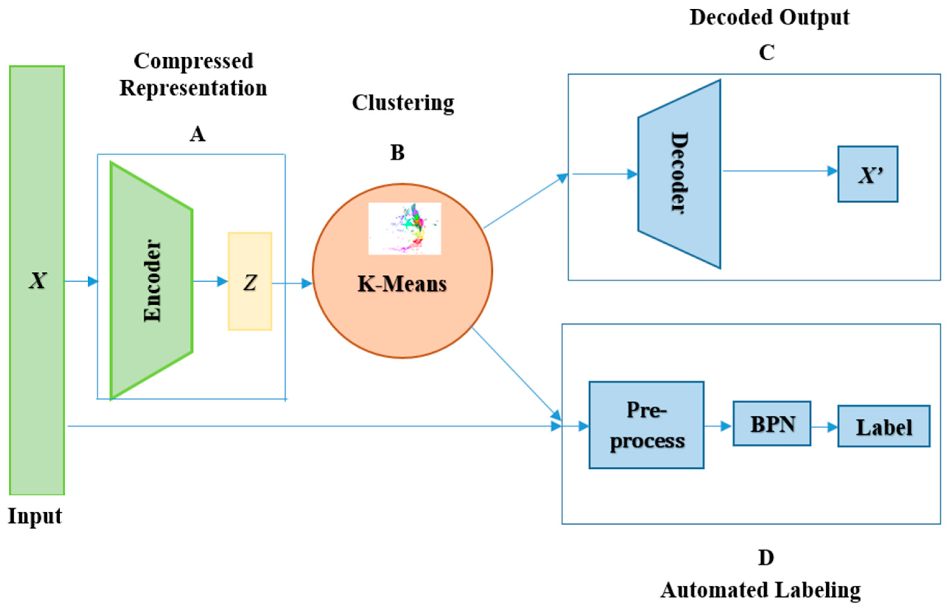
An effective deep learning method, multilayer auto encoders, is proposed in the present research work to label the point cloud data. The neural network pipeline consists of five blocks—input, compressed representation, clustering, decoded output, and automated labeling, as shown in Figure 1.
The methodology uses unsupervised learning, consisting of autoencoders combined with K-means clustering to extract features from the point cloud data for relational class labeling and supervised learning for the segmentation and labeling of the new dataset. The input to the neural network is the point cloud data from LiDAR. Only the highly correlated feature is passed to the compressed representation block. The input features selected for the labeling and segmentation are x, y, and z coordinates with reflectance and distance of the point cloud data. The working of different blocks in Figure 1 is discussed in the below sections.
3.1. Compressed Representation—Block A
Autoencoders are unsupervised networks that learn to compress the inputs [46]. Given the point cloud input , the encoder parameterized with learned to map the input into a fixed latent vector .
Given the unlabeled input dataset = {1, 2, 3,………,n}, where
and n represent the input dimension,
is the lower dimensional hidden encoder vector of size m calculated from as follows:
where
is the weight matrix,
b is the bias of size , and is the linear activation function.
In this approach, is the ReLU activation function, which is defined as follows:
ReLU [43] is the rectified linear activation unit that returns 0 if it receives any negative input but returns that value for any positive value y. Thus, it gives an output that has a range from zero to infinity.
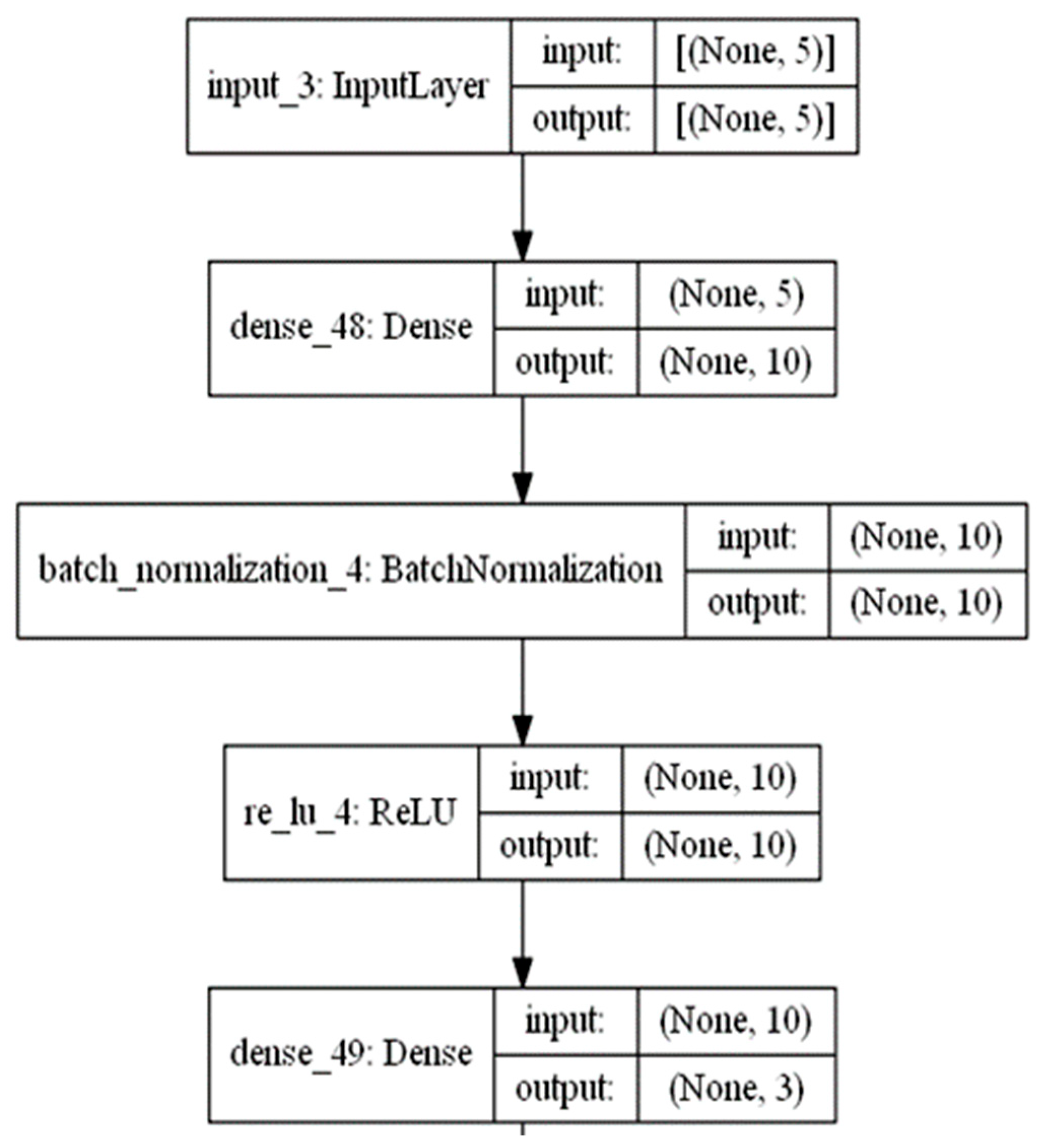
We defined the encoder as having five features as input data; the hidden layer having two times the number of inputs (e.g., 10), followed by the bottleneck layer being reduced to three inputs, as shown in Figure 2. We used batch normalization and ReLU activation to ensure the model learns well. K. Inoue’s [47] experimental analysis shows the expressive power of the ReLU activation function in the neural network.
3.2. Clustering—Block B
The K-means is one of the unsupervised learning algorithms used to classify a given data set through a certain number of clusters, when with cluster centers.
The distance between the cluster center and the data points is calculated as follows:
By updating the centroid for each set of , is the length of the data in the cluster.
The objective function of the clustering algorithm is given below.
The latent-vector is clustered to with as the cluster center using a K-means algorithm, where k represents the number of clusters. The pseudo labeling of clusters is explained in Algorithm 1.
| Algorithm 1: K-Means Clustering Algorithm |
 |
3.3. Decoded Output—Block C
The decoder learns to recreate the data points from the latent space. From the clustered latent-vector , the decoder parameterized with learned to reconstruct the point cloud input that is similar to vector .
The decoding network is similar to the encoder but with different weight, bias, and activation functions as follows:
where is the reconstructed vector, is the clustered latent vector as shown in Equation (5), is the weight matrix of size , is the bias of size , and is the ReLU activation function.
The loss function used to train the AE network through the standard BPN procedure can then be written in terms of these network functions, as given below.
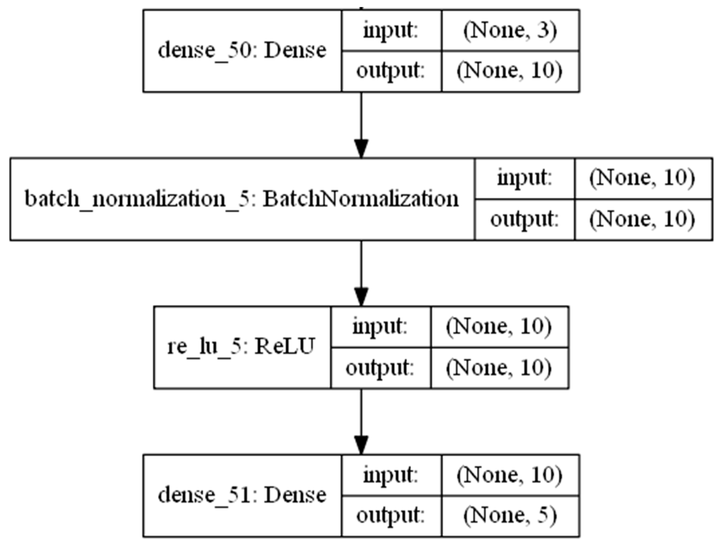
The decoder is similar to the encoder structure, where the input layer is taken over by the latent attributes, as shown in Figure 3. The model is fitted using the efficient Adam version of the stochastic gradient descent [48] to minimize the mean squared error, given that reconstruction is a classification problem.
3.4. Automated Labeling—Block D
The clustered dataset in the latent space is mapped back to the input dataset .
where k represents the number of clusters and j ∈ [1, k].
The dataset is placed in the labeled dataset sample space as follows:
the dataset is divided into a train-test ratio of 70:30. The 70% dataset is used to train the BPN network, and 30% dataset is used to test the model. One must let be a single sample in . After preprocessing, the data sample is represented as follows:
where
represents the region description of based on the ground truth label given in the original A2D2 dataset;
where represents the number of clusters.
The trained model is tested using the dataset. The region-based labels generated by the model are evaluated and placed in the sample space as follows:
where m is the number of labeled point cloud datasets.
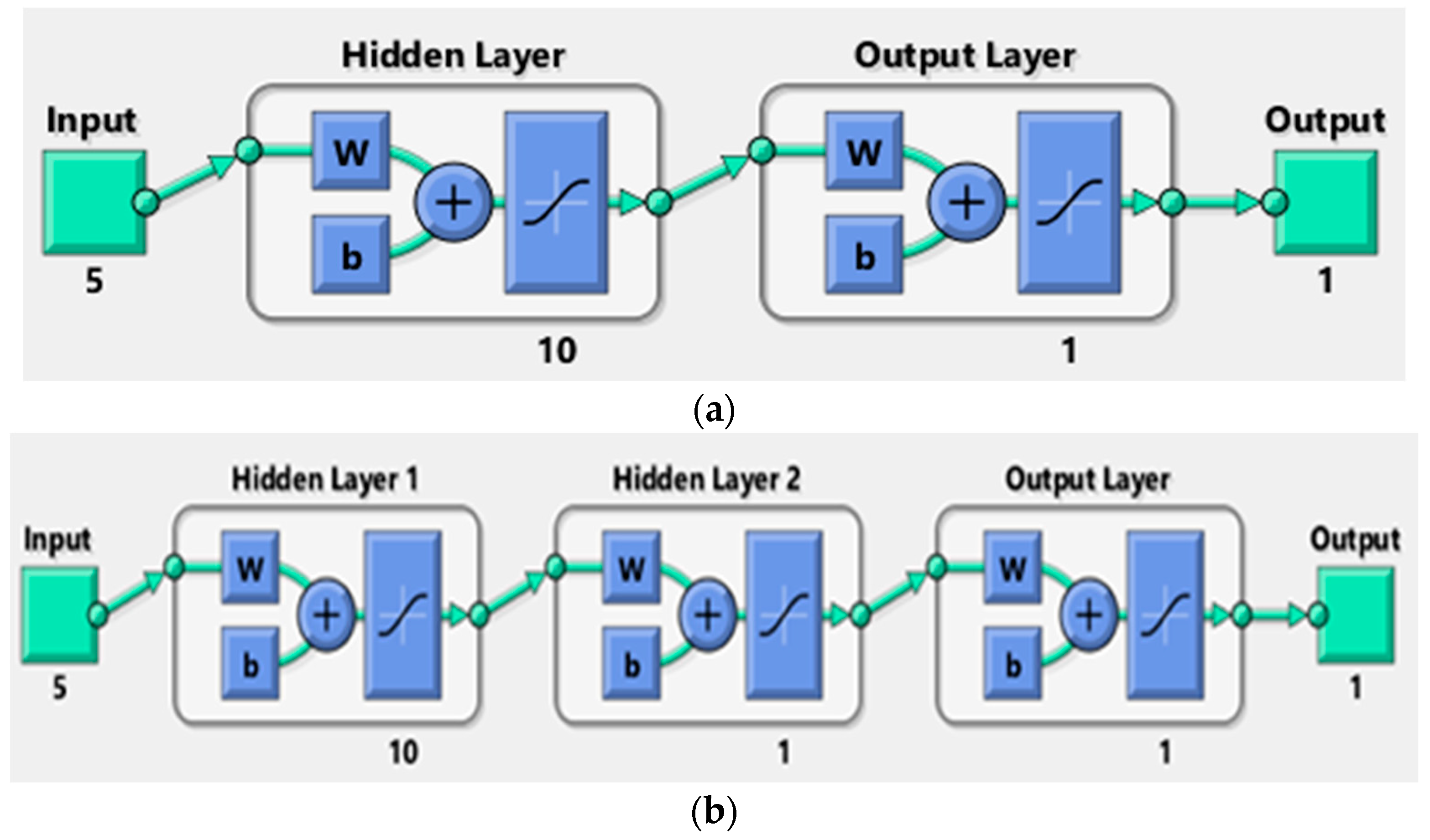
The two-layer BPN shown in Figure 4a has five nodes as input, ten nodes in the hidden layer, and is connected to the output layer. The three-layer BPN, as shown in Figure 4b, has five nodes as input, ten nodes in its first hidden layer, one node in its second hidden layer, and is connected to the output layer. The number of hidden nodes ranged from the number of input features. The sigmoid transfer function is used as an activation function.
3.5. Label Evaluation
In traditional supervised learning, the model performance is evaluated using various metrics, such as precision, recall, F1-score, receiver operating characteristic, and other traditional indicators. However, the performance evaluation in the multilabel learning model is much more complex because each label can be associated with multiple classes simultaneously. The dataset label is not only time-consuming; even if we collect it, it also does not cover all the scenarios. The evaluation of the model using an unlabeled test data set is critical. Some of the benchmark performance evaluation metrics are given in [49].
Microaveraging is one of the evaluation methods to measure the network’s performance. In the microaveraging method, all the true positives (TPs), false positives (FPs), and false negatives (FNs) of each class in the scenes are summed up, and then the average is taken as given in the below equations.
4. Results
The configuration files and the point cloud data are read using the python NumPy library, and exploratory analysis is performed using the python cloud library [50]. The proposed methodology is demonstrated using scenes recorded from different places.
4.1. Dataset
The A2D2 dataset [4,51] includes LiDAR, image, and bus data in the streaming sequences, recorded on highways, country roads, and cities in the south of Germany. The A2D2 dataset contains data collected from five LiDAR sensors, including ‘front left’, ‘front center’, ‘front right’, ‘rear right’, and ‘rear left’, six cameras, including ‘front left’, ‘front center’, ‘front right’, ‘side right’, ‘rear center’ and ‘side left’, and bus signals. The whole data are arranged in frames in the order of the time sequences and also define the view with the frame of reference to the ego vehicle.
Each sensor in ‘lidars’, ‘cameras’, and ‘vehicles’ has an associated ‘view’. A view is a sensor coordinate system defined by an origin, an x-axis, and a y-axis. These are specified in Cartesian coordinates (in m) relative to an external coordinate system. The external coordinate system is the car’s frame of reference. The ego vehicle contains a ‘view’ object describing the sensor’s pose for the car’s frame of reference. It also contains an ‘ego-dimension’ object, which specifies the vehicle’s extension in the car’s frame of reference. The configuration files are stored in a ‘JSON’ file and LiDAR data in the ‘npz’ format. Table 1 describes the LiDAR parameters recorded by the sensors.
The dataset contains semantic, instance segmentation labels, and 3D bounding boxes for 38 categories. A total of 41,277 camera images are semantically labeled, with each pixel representing a semantic category, of which 12,497 are annotated with 3D bounding boxes within the front-center camera field of view. In addition, 3D bounding boxes are estimated by human annotators, including various vehicles, pedestrians, and other relevant objects.
4.2. Model Feature Selection
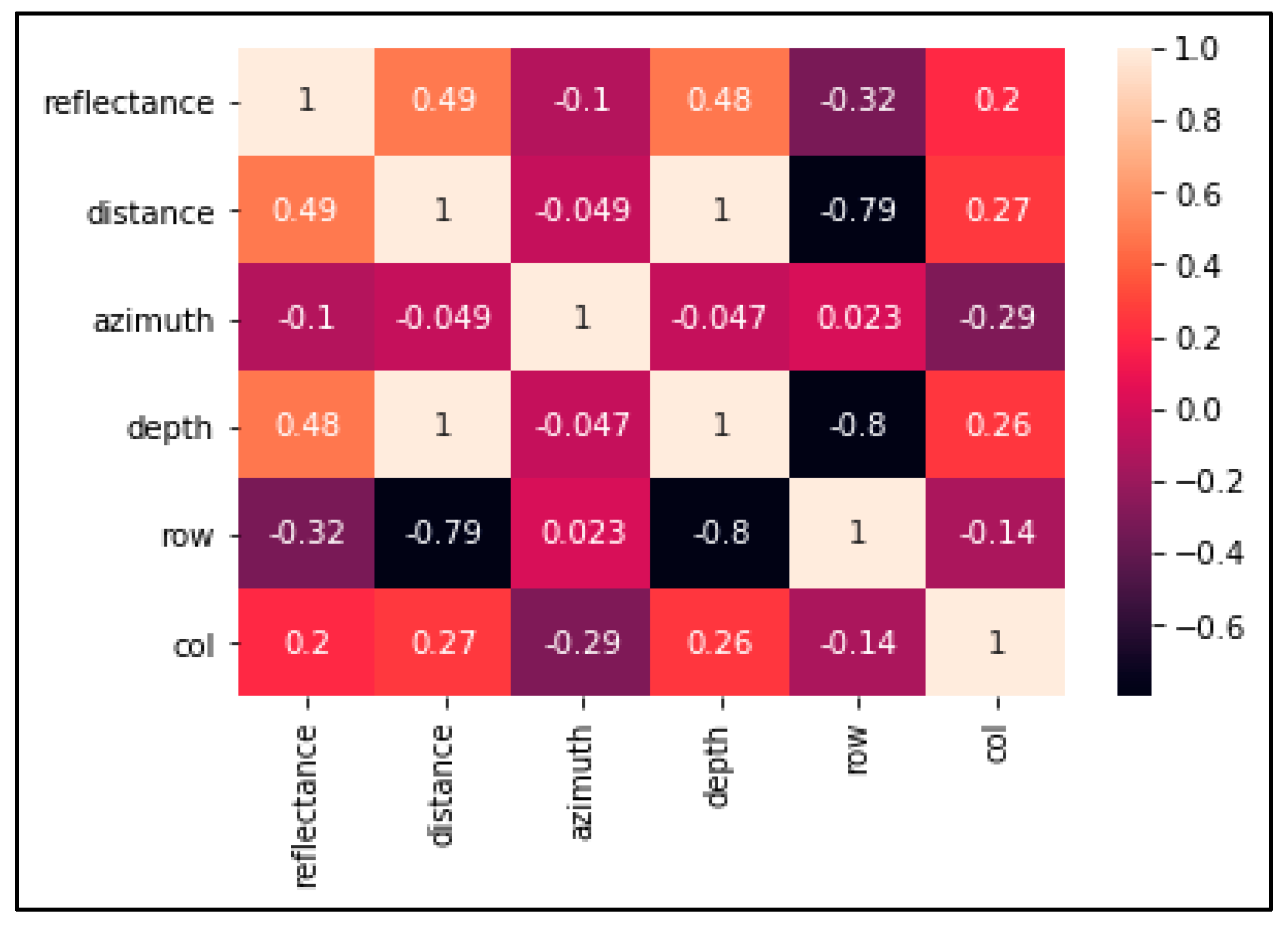
The silhouette value is used to measure the clustering quality [52]. The silhouette score reaches its global maximum at the optimal value of K = 10. We used a correlation matrix to investigate the dependencies between the multiple variables. Based on the correlation matrix plot shown in Figure 5, the features’ distance and depth are highly correlated with the coefficient of 1.0, and reflectance and length are medially correlated with 0.49. Hence, we selected the five features X, Y, Z, reflectance, and distance as the input to the autoencoders. The point cloud data are filtered using the height and reflectance as proposed in the literature [18]. LiDAR point data are filtered with a Z value greater than or equal to −1.0 m (Z ≥ −1.0). The unfiltered points are clustered as road points from the procedure. This filtering procedure also downsamples the data points into a much lower dimension.
4.3. Autoencoder Training Process
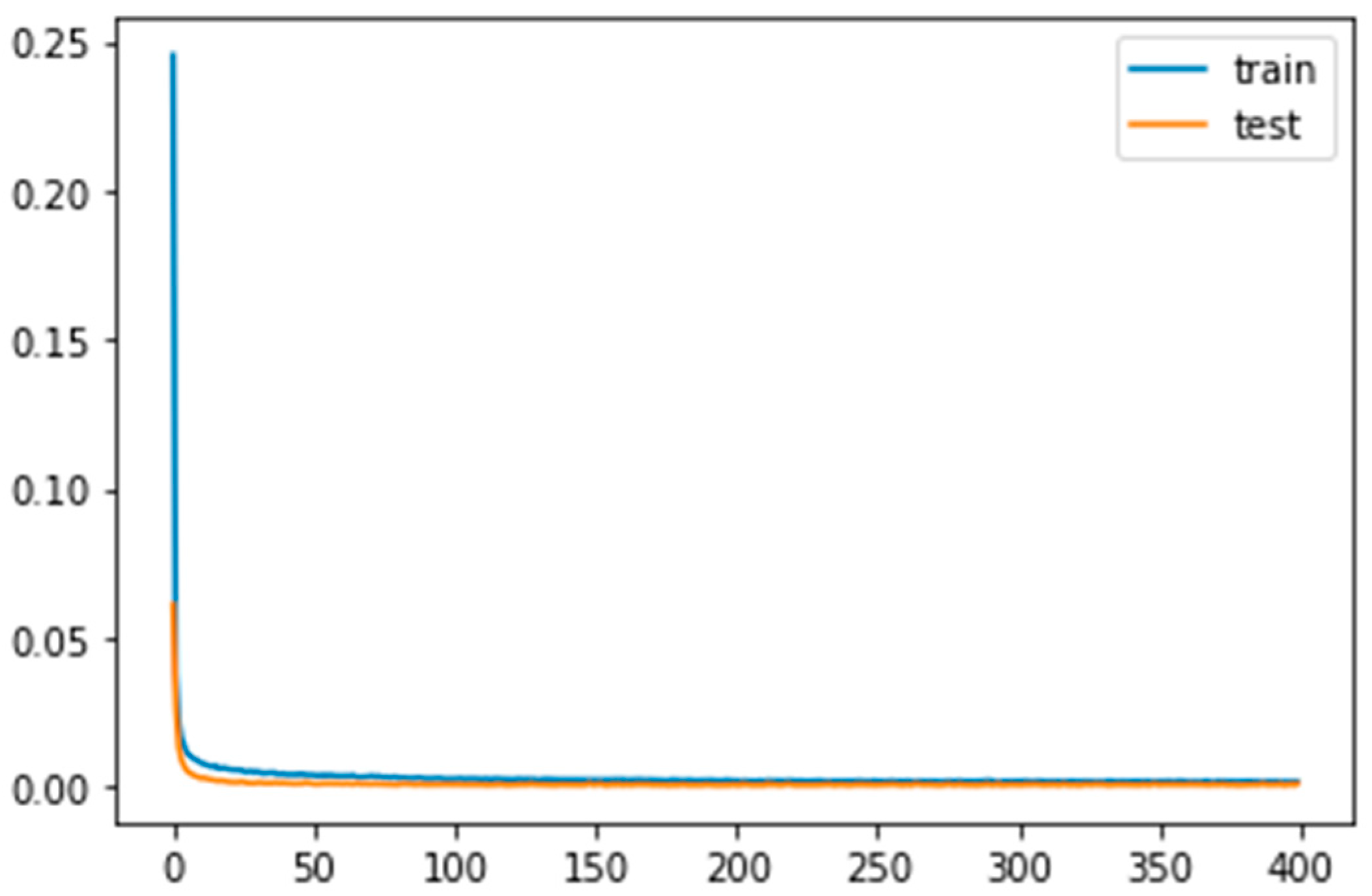
The AE is trained for 50 epochs with the Adam optimizer [21] and implemented binary cross-entropy as a loss function in the network. The parameter batch size was set to 128 during training and 1 during prediction. The training process was computed on NVIDIA GTX 1080ti GPU with l6Gb of RAM. The necessary python modules, such as tensor flow [51], Keras [53], Pandas, OpenCV, and cv2, are imported. The point cloud dataset is converted to Pandas data frame for the analysis and normalized all values between 0 and 1. The dataset is split into 65% for training and 35% for testing. After 30 epochs, the AE seems to reach a stable train and test loss value of about 0.02, as shown in Figure 6.
4.4. BPN Model Training
The proposed BPN model is implemented using MATLAB R2020b. The simulations are performed on an Intel (R) Core (TM) i7-8700K CPU at a 3.70 GHz clock speed with 16 GB RAM. The model learning cycle ranged from 200 to 500 epochs. The learning rate is adaptable with the gradient boosting method for the mean square error loss function, and the momentum(mu) is set at 0.9.
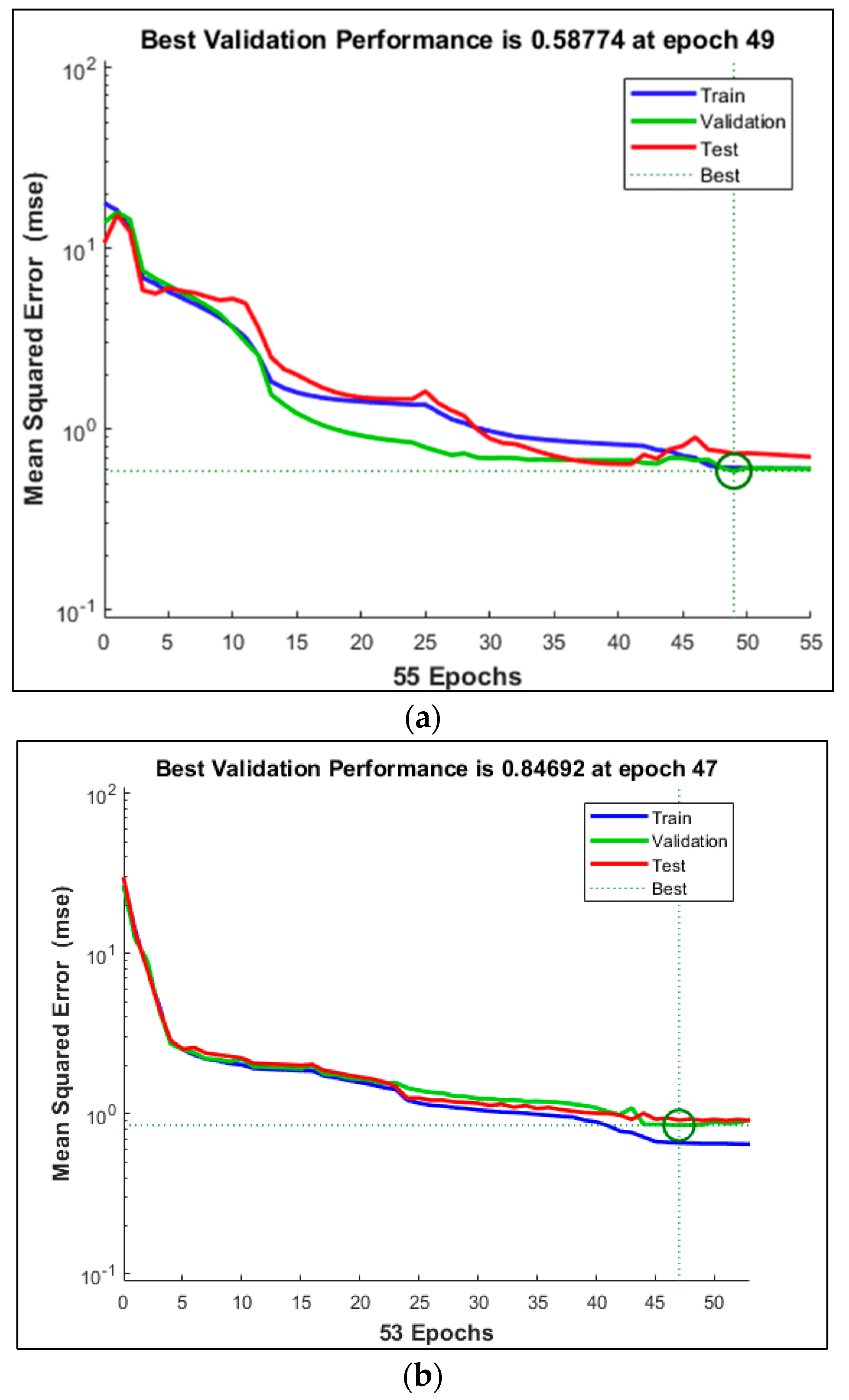
Figure 7a,b show the performance of the BPN two-layer and three-layer networks. The two-layer and three-layer networks became stable at 47 epochs with the best loss values of 0.58 and 0.846, respectively.
4.5. Hyperparameter Tuning
Our 3D labeling and segmentation neural network architecture consists of block A—encoders, block B—K-means, block C—decoder, and block D—BPN. Table 2 describes the details of the parameters in the experiment. In the first stage, we randomly sample N = 15K points from the entire point cloud of A2D2 autonomous driving scenes. After filtering the non-ground points, the subsampled point N = 1024 is passed to the training. We train the autoencoder, block A and block C end to end with the Adam optimizer, with a batch size of 128 and an initial learning rate of 0.01. Its training length is 400 epochs, but the optimal epoch value is 50 based on low training loss. The value is 0.0022, as shown in Figure 6.
We measured the clustering quality by varying the K value for the subsequent clustering of samples in the latent space with K-means in block B and using the silhouette value to find the similarity between the points in the individual cluster. We found that the silhouette score reached its global maximum at the optimal value of K = 10. We stopped the K-means when the centroids of newly formed clusters did not change. K-means is used only in the training phase for labeling, and the time complexity is less than O (KN). We train the BPN, block D end to end with the gradient descent optimizer with a learning rate set to 0.001. Its training length is 200 epochs, but the optimal epoch value is achieved at 47, since the model achieves a low mean square error (MSE) value of 0.6, as shown in Figure 7.
5. Discussion
In the present experiment, we trained autoencoders to cluster objects in the road scene using the data from the front center LiDAR fit in the autonomous vehicle. Moreover, the computer vision might have an ample supply of labeled images. For LiDAR point cloud data, obtaining labels for some fields is highly costly and laborious. Thus, unsupervised clustering of data is indeed a necessity in 3D space. The latent vector’s encoded output is sent to the K-means (k = 10) module for clustering. The clustered data are labeled by filtering the non-ground data with a Z value (Z ≥ −1.0), indicating the objects/obstacles above the road surface.
5.1. Unsupervised Feature Learning of Encoder and Decoder
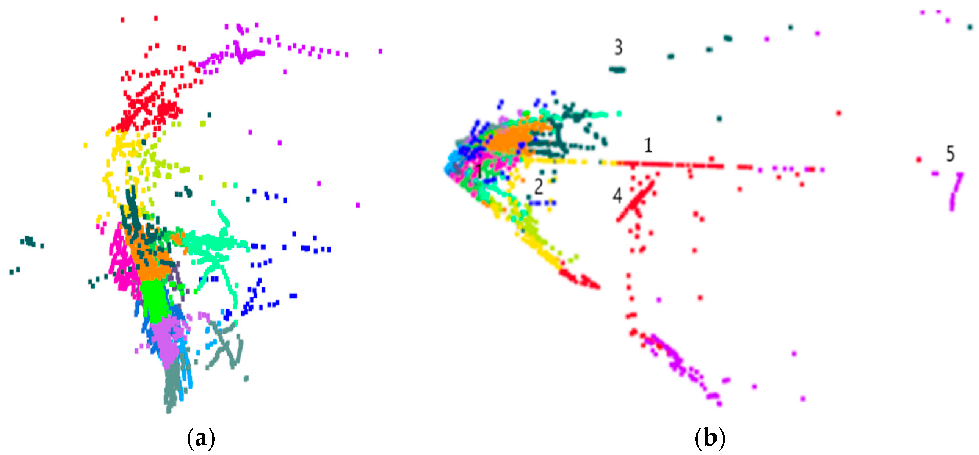
In the unsupervised setting, the number of clusters within the data is not always obvious, especially when some classes may split into multiple clusters or multiple classes sent to the same cluster. Hence, decoding the image after K-means clustering in the latent space is comparatively more beneficial for labeling or identifying the data patterns. The visualization of neighborhoods of different classes on the latent space after clustering is shown in Figure 8a.
The decoded output given in Equation (8) is shown in Figure 8b. The model achieves a good fit in reconstructing the input, as shown in Figure 8b. As we know from the literature, labeled data for different geographical conditions are extremely rare for road scenes. Multiple output frames can be generated from the latent space without missing essential input features. Although the decoded input looks different from the ground truth image, the AE does learn important non-ground objects, dividers (1), cars (2–4), and trucks (5), as marked in Figure 8b.
Figure 8a shows the encoded and clustered output of block C, and Figure 8b is the decoded output of block C, synthesized point cloud data. This synthesized data from block C can be included in the training data for the model’s generalizability to detect new scenes. The current proposal is limited to real-time data.
5.2. Pseudo Labeling
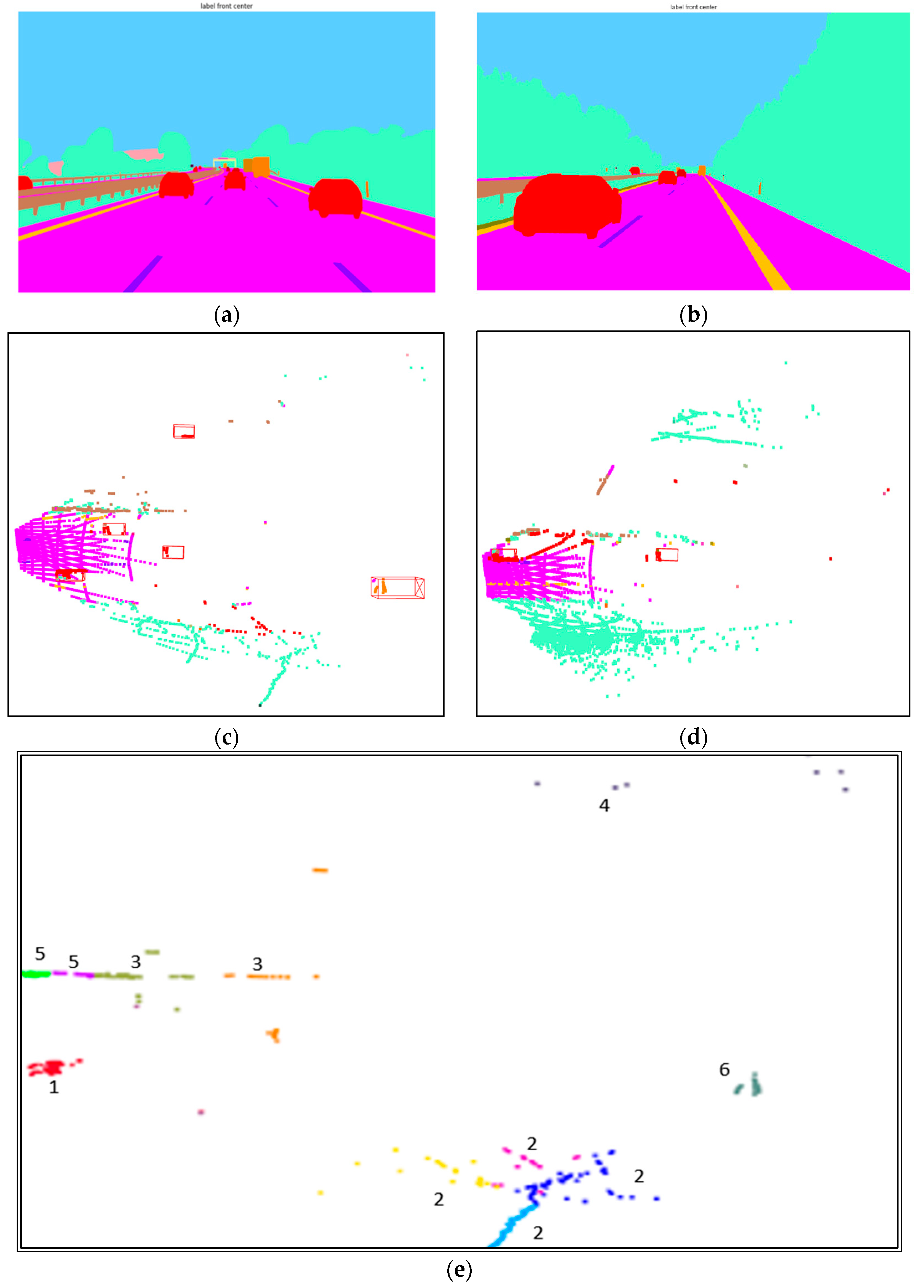
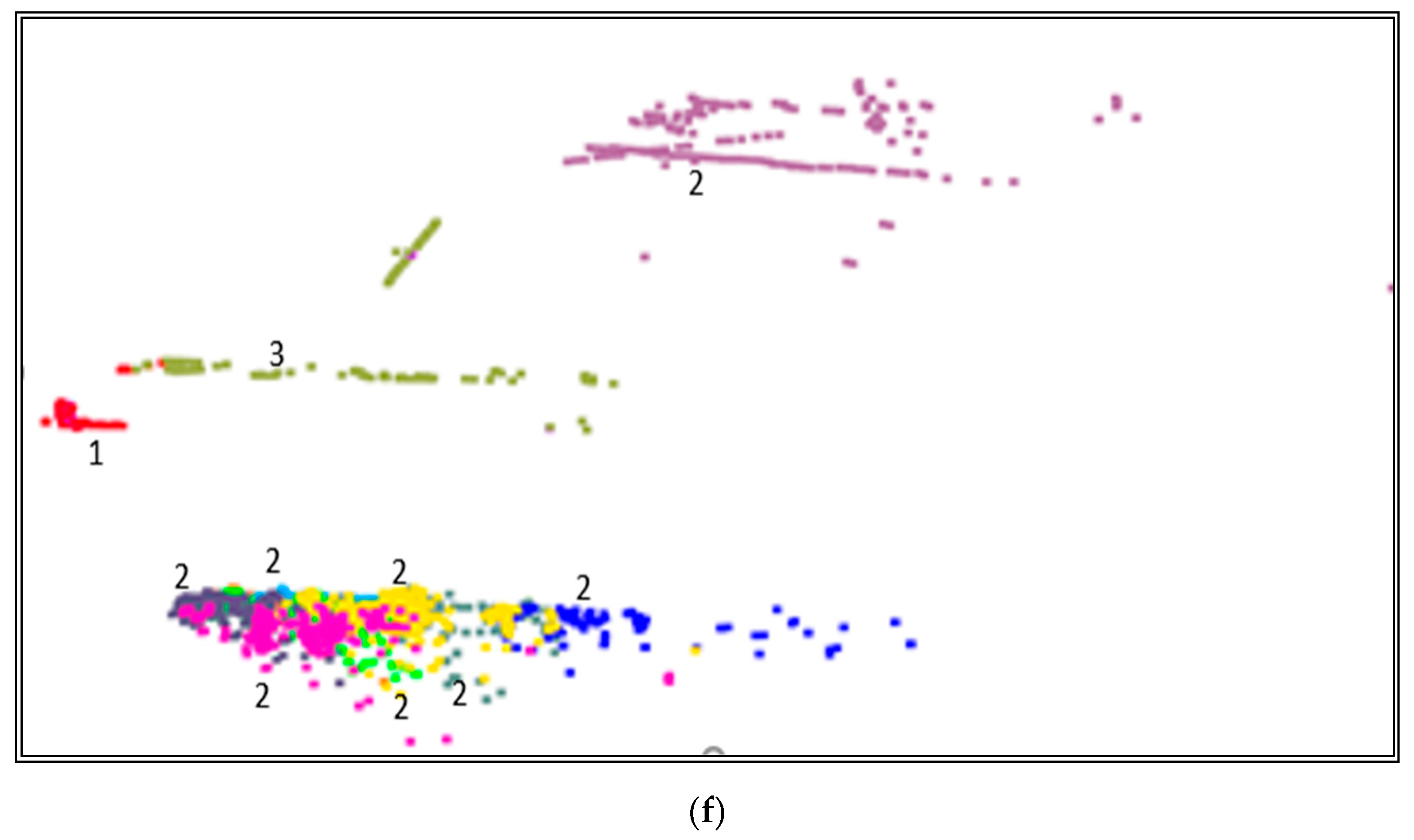
Figure 9a,b shows the ground truth segmentation of camera images. Figure 9c,d show the BEV’s corresponding LiDAR point cloud data segmentation. The bounding boxes show the vehicles in the road scene matching the color codes given in the segmented camera images in Figure 9b. The pseudo-labeling of the non-ground data using AE and K-means is shown in Figure 9f. The pseudo labels are shown in different colors and converted to relational labels using ground truth segmentation.
Table 3 shows the six categories of relational labels. The pseudo labels in Figure 9e, f is marked with different labels, as given in Table 3.
The 3D point cloud data segmentation with the class labels’ description shows the unified annotations of multiple classes coexisting in the same scene and the deep learning techniques proposed in the present study evolve with increasing training data.
5.3. Generating Automated Labeling and Segmentation Using BPN Network
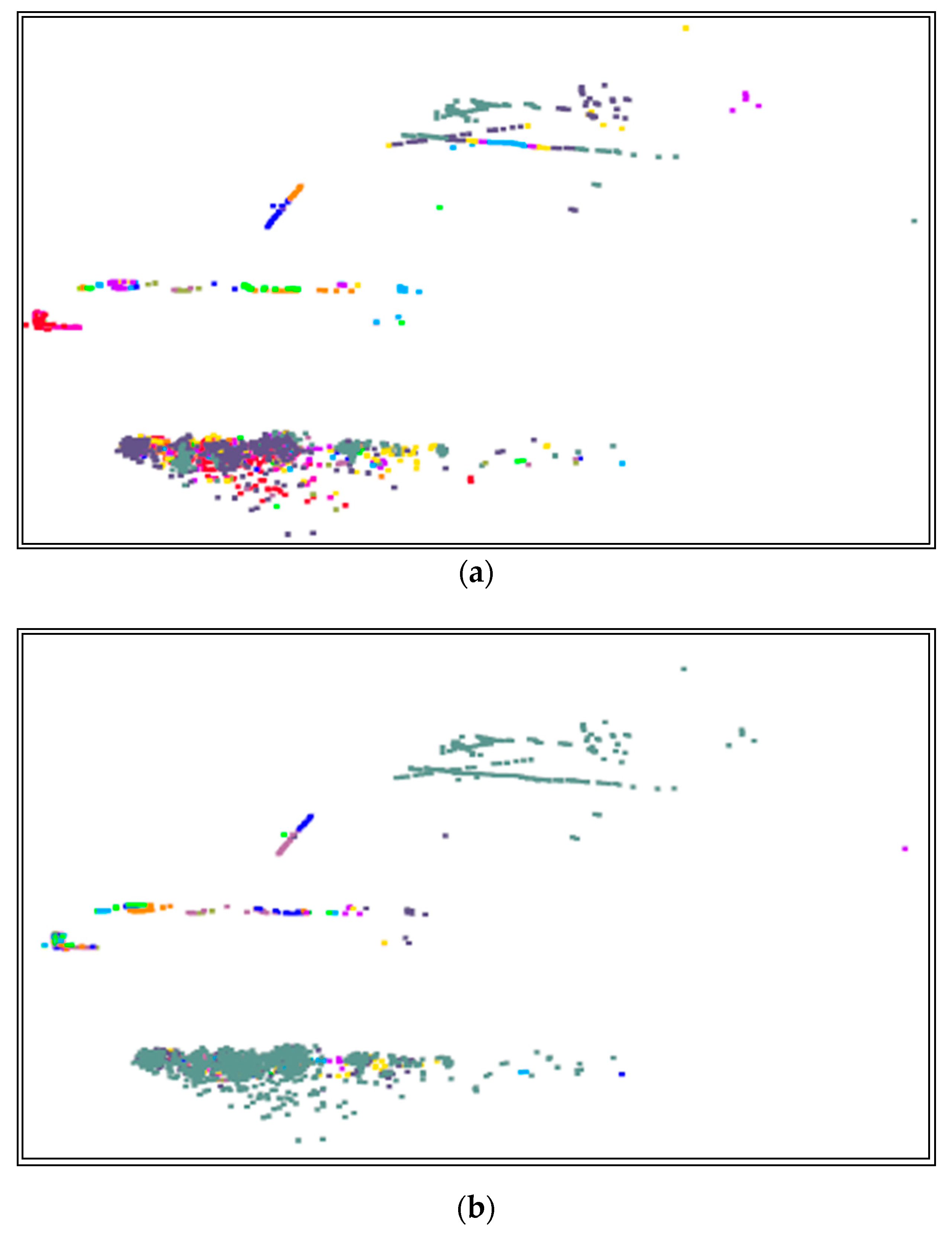
The learning algorithm for one-hidden-layer feedforward neural networks can learn any set of observations in one short iteration, instead of many learning epochs with acceptable learning and testing accuracy, as shown in Figure 10. The network’s learning shows that any continuous bounded activation functions can form disjoint decision regions in multidimensional cases, as discussed in the literature [43]. The output of the two-layer BPN shown in Figure 10a performed better than the three-layer BPN shown in Figure 10b as it was able to label the car, vegetation, divider, and the car next to vegetation. In the case of three-layer BPN, the network mislabeled the car and divider as vegetation.
5.4. Evaluation of Segmentation (Supervised Learning)
The evaluation of automated labeling and semantic segmentation here uses the method similar to [54]. In multilabel classification, a misclassification of FPs is better than the no prediction of FNs. The false-positive counts help to optimize algorithms for the misclassified classes. The precision, recall, and F1 score are calculated based on the Equations (14)–(16), respectively, which are listed in Table 4. The model accuracy is calculated based on the Equation (17). The BPN two-layer model performed the best with an accuracy of 75%.
To gain deeper insight into our model, we provided several typical cases where our approach fails on the A2D2 dataset. In Figure 10, we illustrate the labeling for different semantic categories. As observed in the output, the failures are mainly due to (i) incorrect recognition as a result of some similar pattern between the object classes (e.g., vegetation and divider) or (ii) misclassified small or occluded objects (e.g., truck or car). We compared our result with other state-of-art methods in a similar field of study. In group-wise learning [16], the segmentation accuracy of images is 68.7%; for point cloud, weakly supervised segmentation with fewer labels [10], the segmentation accuracy of a real-time point cloud dataset S3DIS (Area 5) is 48.0%. In the same study area as ours, the accuracy of different datasets shows that more labeling techniques are required to improve the segmentation task for group-wise learning with unsupervised learning methods.
6. Conclusions
In the present research, 3D point cloud data labeling is considered semi-supervised learning, as it is streamlined using both unsupervised and supervised learning models. The geometric properties of data lie in the lower dimension rather than the actual input space, and each data point has a set of neighbors connected by Euclidean distance. In the proposed architecture, the unsupervised learning model labels the poorly labeled data into the relational label. Dimension reduction is much better than the down-sampling techniques, since it preserves spatial information without losing the data patterns. The experiment reduces the original point cloud data dimensionality to 30% using autoencoders. The decoder generates new images, and K-means creates the subset named pseudo labels of the n-dimensional Euclidean space. The synthesized image can help improve the generalizability property of the model for segmenting new scenes.
Each pseudo label is compared with the ground truth and converted into relational labels. These relational labels are also called class labels. The backpropagation feedforward neural networks are trained using these class labels to label the unlabeled data. The labels are evaluated by finding the true positive, false positive, and false negative. To improve accuracy, the supervised model uses multiple learning iterations with more labeled data and optimization techniques. The two-layer BPN model performed better than the three-layer BPN model.
The synthesized data can also be included in training the BPN models for future investigations. The study offers an opportunity to improve the methodology or application further to merge multiple frame receivers from other sensors by observing similarities and dissimilarities, and labeling the relationship between different frames. While the present work focuses on clustering and labeling models from BEV, it is possible to extend the models to incorporate data across multiple views from LiDAR. By including point cloud augmentation algorithms, rotation, and homogenous transformation matrixes, we can change the viewpoint to a global coordinate system in the model hyper parameters, and integrate AE with rotational and angle invariant transformer networks, such as spatial transformer and T-net models.
The labeled dataset can be used in supervised learning for scene segmentation. One of the downsides of the methodology is that we have to create our initial clusters based on the data encoded by the untrained network. The clusters may not necessarily be as accurate but can still produce semantically meaningful groupings. Another downside of the method is that it requires the number of clusters as a hyper parameter. In the future, the approach can be extended to incorporate graphical neural networks to learn the relationship between the neighboring points using node classification and segmentation.
Author Contributions
Conceptualization, V.S.S. and H.Y.; Data curation, R.-C.C. and V.S.S.; Formal analysis, R.-C.C., V.S.S., L.-S.C. and H.Y.; Funding acquisition, R.-C.C. and L.-S.C.; Investigation, R.-C.C., V.S.S. and H.Y.; Methodology, V.S.S.; Project administration, R.-C.C. and L.-S.C.; Software, V.S.S. and H.Y.; Supervision, R.-C.C. and L.-S.C.; Validation, R.-C.C. and V.S.S.; Visualization, V.S.S.; Writing—original draft, V.S.S.; Writing—review & editing, R.-C.C. All authors have read and agreed to the published version of the manuscript.
Funding
This paper is funded by the Ministry of Science and Technology, Taiwan. The No.s are MOST-110-2927-I-324-50, MOST-110-2221-E-324-010 and MOST-109-2622-E-324-004, Taiwan.
Institutional Review Board Statement
Not applicable.
Informed Consent Statement
Not applicable.
Data Availability Statement
Acknowledgments
The authors would like to thank Lata Ganesan, Sr. Data Scientist, for editing, proofreading and evaluating the contents of the paper.
Conflicts of Interest
The authors declare no conflict of interest.
References
- Cleary, A.; Yoo, K.; Samuel, P.; George, S.; Sun, F.; Israel, S.A. Machine Learning on Small UAVs. In Proceedings of the 2020 IEEE Applied Imagery Pattern Recognition Workshop (AIPR), Washington, DC, USA, 13–15 October 2020; pp. 1–5. [Google Scholar] [CrossRef]
- Kuutti, S.; Fallah, S.; Katsaros, K.; Dianati, M.; Mccullough, F.; Mouzakitis, A. A Survey of the State-of-the-Art Localization Techniques and Their Potentials for Autonomous Vehicle Applications. IEEE Internet Things J. 2018, 5, 829–846. [Google Scholar] [CrossRef]
- Bhattacharyya, A.; Reino, D.O.; Fritz, M.; Schiele, B. Euro-PVI: Pedestrian Vehicle Interactions in Dense Urban Centers. 2021. pp. 6404–6413. Available online: http://arxiv.org/abs/2106.12442 (accessed on 6 May 2022).
- Geyer, J.; Kassahun, Y.; Mahmudi, M.; Ricou, X.; Durgesh, R.; Chung, A.S.; Hauswald, L.; Pham, V.H.; Mühlegg, M.; Dorn, S.; et al. A2D2: Audi Autonomous Driving Dataset. arXiv 2020, arXiv:2004.06320. [Google Scholar]
- Riegler, G.; Ulusoy, A.O.; Geiger, A. OctNet: Learning Deep 3D Representations at High Resolutions. In Proceedings of the IEEE Conference on Computer Vision and Pattern Recognition (CVPR), Honolulu, HI, USA, 21–26 July 2017; pp. 6620–6629. [Google Scholar] [CrossRef] [Green Version]
- He, Q.; Wang, Z.; Zeng, H.; Zeng, Y.; Liu, Y. Svga-net: Sparse voxel-graph attention network for 3d object detection from point clouds. In Proceedings of the AAAI Conference on Artificial Intelligence 2020, New York, NY, USA, 7–12 February 2020. [Google Scholar]
- Wang, S.; Sun, Y.; Liu, C.; Liu, M. PointTrackNet: An End-to-End Network For 3-D Object Detection and Tracking from Point Clouds. IEEE Robot. Autom. Lett. 2020, 5, 3206–3212. [Google Scholar] [CrossRef] [Green Version]
- Huang, J.; You, S. Point cloud labeling using 3D Convolutional Neural Network. In Proceedings of the 2016 23rd International Conference on Pattern Recognition (ICPR), Cancún, Mexico, 4–8 December 2016; pp. 2670–2675. [Google Scholar] [CrossRef]
- Caine, B.; Roelofs, R.; Vasudevan, V.; Ngiam, J.; Chai, Y.; Chen, Z.; Shlens, J. Pseudo-Labeling for Scalable 3D Object Detection. 2021. Available online: http://arxiv.org/abs/2103.02093 (accessed on 16 April 2022).
- Xu, X.; Lee, G.H. Weakly supervised semantic point cloud segmentation: Towards 10x fewer labels. In Proceedings of the IEEE/CVF conference on computer vision and pattern recognition, Seattle, WA, USA, 13–19 June 2020; pp. 13703–13712. [Google Scholar] [CrossRef]
- Qin, Z.; Wang, J.; Lu, Y. Weakly Supervised 3D Object Detection from Point Clouds. In Proceedings of the 28th ACM International Conference on Multimedia, Seattle, WA, USA, 12–16 October 2020; pp. 4144–4152. [Google Scholar] [CrossRef]
- Zhou, T.; Wang, W.; Konukoglu, E.; Van Gool, L. Rethinking Semantic Segmentation: A Prototype View. In Proceedings of the IEEE/CVF Conference on Computer Vision and Pattern Recognition, New Orleans, LA, USA, 19–24 June 2022. [Google Scholar]
- Guinard, S.; Landrieu, L. Weakly supervised segmentation-aided classification of urban scenes from 3D LiDAR point clouds. In Proceedings of the ISPRS, Hannover, Germany, 6–9 June 2017; Volume 42, pp. 151–157. [Google Scholar] [CrossRef] [Green Version]
- Belkin, M.; Niyogi, P.; Sindhwani, V. Manifold Regularization: A Geometric Framework for Learning from Labeled and Unlabeled Examples. J. Mach. Learn. Res. 2006, 7, 2399–2434. [Google Scholar]
- Zhou, Z.-H. A brief introduction to weakly supervised learning. Natl. Sci. Rev. 2017, 5, 44–53. [Google Scholar] [CrossRef] [Green Version]
- Zhou, T.; Li, L.; Li, X.; Feng, C.-M.; Li, J.; Shao, L. Group-Wise Learning for Weakly Supervised Semantic Segmentation. IEEE Trans. Image Process. 2021, 31, 799–811. [Google Scholar] [CrossRef] [PubMed]
- Feng, M.; Gilani, S.Z.; Wang, Y.; Zhang, L.; Mian, A. Relation Graph Network for 3D Object Detection in Point Clouds. IEEE Trans. Image Process. 2020, 30, 92–107. [Google Scholar] [CrossRef]
- Choi, Y.-W.; Jang, Y.-W.; Lee, H.-J.; Cho, G.-S. Three-Dimensional LiDAR Data Classifying to Extract Road Point in Urban Area. IEEE Geosci. Remote Sens. Lett. 2008, 5, 725–729. [Google Scholar] [CrossRef]
- Douillard, B.; Underwood, J.; Kuntz, N.; Vlaskine, V.; Quadros, A.; Morton, P.; Frenkel, A. On the segmentation of 3D LIDAR point clouds. In Proceedings of the IEEE International Conference on Robotics and Automation, Shanghai, China, 9–13 May 2011; pp. 2798–2805. [Google Scholar] [CrossRef]
- Zhou, B.; Lapedriza, A.; Xiao, J.; Torralba, A.; Oliva, A. Learning Deep Features for Scene Recognition using Places Database—Supplementary Materials. In Proceedings of the 27th International Conference on Neural Information Processing Systems NIPS’14, Montreal, QC, Canada, 8–13 December 2014; Volume 1, pp. 487–495. [Google Scholar]
- Xu, X.; Li, W.; Xu, D.; Tsang, I.W. Co-Labeling for Multi-View Weakly Labeled Learning. IEEE Trans. Pattern Anal. Mach. Intell. 2015, 38, 1113–1125. [Google Scholar] [CrossRef]
- Bengio, Y.; Courville, A.; Vincent, P. Representation Learning: A Review and New Perspectives. IEEE Trans. Pattern Anal. Mach. Intell. 2013, 35, 1798–1828. [Google Scholar] [CrossRef] [PubMed]
- Xiong, Z.; Yuan, Y.; Wang, Q. RGB-D Scene Recognition via Spatial-Related Multi-Modal Feature Learning. IEEE Access 2019, 7, 106739–106747. [Google Scholar] [CrossRef]
- Gao, J.; Li, F.; Wang, B.; Liang, H. Unsupervised nonlinear adaptive manifold learning for global and local information. Tsinghua Sci. Technol. 2021, 26, 163–171. [Google Scholar] [CrossRef]
- Gong, M.; Liu, J.; Li, H.; Cai, Q.; Su, L. A Multiobjective Sparse Feature Learning Model for Deep Neural Networks. IEEE Trans. Neural Netw. Learn. Syst. 2015, 26, 3263–3277. [Google Scholar] [CrossRef]
- Rossi, R.A.; Zhou, R.; Ahmed, N.K. Deep Inductive Graph Representation Learning. IEEE Trans. Knowl. Data Eng. 2018, 32, 438–452. [Google Scholar] [CrossRef]
- Tran, S.N.; Garcez, A. Deep Logic Networks: Inserting and Extracting Knowledge from Deep Belief Networks. IEEE Trans. Neural Netw. Learn. Syst. 2016, 29, 246–258. [Google Scholar] [CrossRef] [Green Version]
- Ozdemir, A.O.B.; Gedik, B.E.; Cetin, C.Y.Y. Hyperspectral classification using stacked autoencoders with deep learning. In Proceedings of the 6th Workshop on Hyperspectral Image and Signal Processing: Evolution in Remote Sensing (WHISPERS), Piscataway, NJ, USA, 24–27 June 2014; pp. 1–4. [Google Scholar] [CrossRef]
- Xu, J.; Fang, Z.; Gao, Y.; Ma, S.; Jin, Y.; Zhou, H.; Wang, A. Point AE-DCGAN: A deep learning model for 3D point cloud lossy geometry compression. In Proceedings of the 2021 Data Compression Conference (DCC), Snowbird, UT, USA, 23–26 March 2021; p. 379. [Google Scholar] [CrossRef]
- Tai, S.-K.; Dewi, C.; Chen, R.-C.; Liu, Y.-T.; Jiang, X.; Yu, H. Deep Learning for Traffic Sign Recognition Based on Spatial Pyramid Pooling with Scale Analysis. Appl. Sci. 2020, 10, 6997. [Google Scholar] [CrossRef]
- Dewi, C.; Chen, R.-C.; Tai, S.-K. Evaluation of Robust Spatial Pyramid Pooling Based on Convolutional Neural Network for Traffic Sign Recognition System. Electronics 2020, 9, 889. [Google Scholar] [CrossRef]
- Qi, C.R.; Su, H.; Mo, K.; Guibas, L.J. PointNet: Deep learning on point sets for 3D classification and segmentation. In Proceedings of the IEEE conference on computer vision and pattern recognition, Honolulu, HI, USA, 21–26 July 2017; pp. 77–85. [Google Scholar] [CrossRef]
- Qi, C.R.; Yi, L.; Su, H.; Guibas, L.J. PointNet++: Deep hierarchical feature learning on point sets in a metric space. Adv. Neural Inf. Process. Syst. 2017, 30, 5100–5109. [Google Scholar]
- Achlioptas, P.; Diamanti, O.; Mitliagkas, I.; Guibas, L. Learning representations and generative models for 3d point clouds. In Proceedings of the 35th International Conference on Machine Learning ICML 2018, Stockholm, Sweden, 10–15 July 2018; Volume 1, pp. 67–85. [Google Scholar]
- Dewi, C.; Chen, R.-C.; Liu, Y.-T.; Yu, H. Various Generative Adversarial Networks Model for Synthetic Prohibitory Sign Image Generation. Appl. Sci. 2021, 11, 2913. [Google Scholar] [CrossRef]
- Rios, T.; Wollstadt, P.; Van Stein, B.; Back, T.; Xu, Z.; Sendhoff, B.; Menzel, S. Scalability of Learning Tasks on 3D CAE Models Using Point Cloud Autoencoders. In Proceedings of the IEEE Symposium Series on Computational Intelligence 2019, Xiamen, China, 6–9 December 2019; pp. 1367–1374. [Google Scholar] [CrossRef]
- Anggoro, F.; Caraka, R.E.; Prasetyo, F.A.; Ramadhani, M.; Gio, P.U.; Chen, R.-C.; Pardamean, B. Revisiting Cluster Vulnerabilities towards Information and Communication Technologies in the Eastern Island of Indonesia Using Fuzzy C Means. Sustainability 2022, 14, 3428. [Google Scholar] [CrossRef]
- Xie, J.; Girshick, R.; Farhadi, A. Unsupervised deep embedding for clustering analysis. In Proceedings of the 33rd International Conference on Machine Learning (ICML 2016), New York, NY, USA, 19–24 June 2016; Volume 1, pp. 740–749. [Google Scholar]
- Coates, A.; Lee, H.; Ng, A.Y. An analysis of single-layer networks in unsupervised feature learning. J. Mach. Learn. Res. 2011, 15, 215–223. [Google Scholar]
- Qaiwmchi, N.A.H.; Amintoosi, H.; Mohajerzadeh, A. Intrusion Detection System Based on Gradient Corrected Online Sequential Extreme Learning Machine. IEEE Access 2020, 9, 4983–4999. [Google Scholar] [CrossRef]
- Melnik, O. Decision Region Connectivity Analysis: A Method for Analyzing High-Dimensional Classifiers. Mach. Learn. 2002, 48, 321–351. [Google Scholar] [CrossRef] [Green Version]
- Huang, G.-B.; Chen, Y.-Q.; Babri, H. Classification ability of single hidden layer feedforward neural networks. IEEE Trans. Neural Netw. 2000, 11, 799–801. [Google Scholar] [CrossRef] [Green Version]
- Hu, H.; Cui, Z.; Wu, J.; Wang, K. Metric Learning-Based Multi-Instance Multi-Label Classification with Label Correlation. IEEE Access 2019, 7, 109899–109909. [Google Scholar] [CrossRef]
- Yadavendra; Chand, S. Multiclass and multilabel classification of human cell components using transfer learning of inceptionv3 model. In Proceedings of the 17th International Conference on Intelligent Computer Communication and Processing, Cluj-Napoca, Romania, 28–30 October 2021; pp. 523–528. [Google Scholar] [CrossRef]
- Jamison, T.; Schalkoff, R. Image labelling: A neural network approach. Image Vis. Comput. 1988, 6, 203–214. [Google Scholar] [CrossRef]
- Lapenta, L.V.N.; Monteiro, R.P.; Bastos-Filho, C.J.A. Autoencoder latent space: An empirical study. In Proceedings of the 2020 IEEE Symposium Series on Computational Intelligence, Canberra, Australia, 1–4 December 2020; pp. 2453–2460. [Google Scholar] [CrossRef]
- Inoue, K. Expressive numbers of two or more hidden layer relu neural networks. In Proceedings of the 2019 Seventh International Symposium on Computing and Networking Workshops (CANDARW), Nagasaki, Japan, 26–29 November 2019; pp. 129–135. [Google Scholar] [CrossRef]
- Tao, C.; Pan, H.; Li, Y.; Zou, Z. Unsupervised Spectral–Spatial Feature Learning with Stacked Sparse Autoencoder for Hyperspectral Imagery Classification. IEEE Geosci. Remote Sens. Lett. 2015, 12, 2438–2442. [Google Scholar] [CrossRef]
- Pan, L.; Pipitsunthonsan, P.; Daengngam, C.; Channumsin, S.; Sreesawet, S.; Chongcheawchamnan, M. Identification of Complex Mixtures for Raman Spectroscopy Using a Novel Scheme Based on a New Multi-Label Deep Neural Network. IEEE Sensors J. 2021, 21, 10834–10843. [Google Scholar] [CrossRef]
- A2D2. Available online: https://www.a2d2.audi/a2d2/en/tutorial.html (accessed on 16 April 2022).
- Abadi, M.; Agarwal, A.; Barham, P.; Brevdo, E.; Chen, Z.; Citro, C.; Corrado, G.S.; Davis, A.; Dean, J.; Devin, M.; et al. TensorFlow: Large-Scale Machine Learning on Heterogeneous Systems. 2015. Available online: https://www.tensorflow.org/ (accessed on 16 April 2022).
- Rios, T.; Van Stein, B.; Menzel, S.; Back, T.; Sendhoff, B.; Wollstadt, P. Feature Visualization for 3D Point Cloud Autoencoders. In Proceedings of the 2020 International Joint Conference on Neural Networks (IJCNN), Glasgow, UK, 19–24 July 2020. [Google Scholar] [CrossRef]
- Chollet, F. Keras. 2015. Available online: https://keras.io/ (accessed on 16 April 2022).
- Rottmann, M.; Maag, K.; Chan, R.; Huger, F.; Schlicht, P.; Gottschalk, H. Detection of False Positive and False Negative Samples in Semantic Segmentation. In Proceedings of the Design, Automation & Test in Europe Conference & Exhibition, Grenoble, France, 9–13 March 2020; pp. 1351–1356. [Google Scholar] [CrossRef]
Figure 1.
Neural network architecture pipeline with (A) Compressed Representation, (B) Clustering, (C) Decoded Output and (D) Automated Labeling.
Figure 1.
Neural network architecture pipeline with (A) Compressed Representation, (B) Clustering, (C) Decoded Output and (D) Automated Labeling.

Figure 2.
Encoder flow diagram.

Figure 3.
Decoder flow diagram.

Figure 4.
Backpropagation neural (BPN) network structure for automated label. (a). Two-layer. (b). Three-layer.
Figure 4.
Backpropagation neural (BPN) network structure for automated label. (a). Two-layer. (b). Three-layer.

Figure 5.
Correlation matrix of 3D point cloud data features.

Figure 6.
Train and test losses vs. epochs.

Figure 7.
BPN performance. (a). Two-layer. (b). Three-layer.

Figure 8.
Output of encoder and decoder. (a). Point cloud clusters in latent space; (b). decoded output of point cloud data.
Figure 8.
Output of encoder and decoder. (a). Point cloud clusters in latent space; (b). decoded output of point cloud data.

Figure 9.
Ground truth segmentation and pseudo labels. (a). Ground-truth image; (b). ground-truth image; (c). ground-truth point cloud data; (d). ground-truth point cloud data; (e). sample point cloud pseudo labels; (f). sample point cloud pseudo labels.
Figure 9.
Ground truth segmentation and pseudo labels. (a). Ground-truth image; (b). ground-truth image; (c). ground-truth point cloud data; (d). ground-truth point cloud data; (e). sample point cloud pseudo labels; (f). sample point cloud pseudo labels.


Figure 10.
Labeling and segmentation output on the test data using BPN (supervised learning). (a). Labeling and segmentation with two-layer BPN. (b). Labeling and segmentation with three-layer BPN.
Figure 10.
Labeling and segmentation output on the test data using BPN (supervised learning). (a). Labeling and segmentation with two-layer BPN. (b). Labeling and segmentation with three-layer BPN.


Table 1.
Point cloud features.
| Parameters | Description |
|---|---|
| X | X location in the world coordinate system |
| Y | Y location in the world coordinate system |
| Z | Z (elevation) location in the world coordinate system |
| Azimuth | The angle between the reference plane and the point |
| Distance | Distance of the point from the car’s frame of reference |
| Row | Pixel height location of the point in RGB camera image |
| Col | Pixel width location of the point in RGB camera image |
| Depth | Depth of the corresponding camera image |
| Reflectance | Reflection of the object |
| Timestamp | The time is taken by the reflected light |
Table 2.
A concise list of selected hyperparameters for modules in neural network architecture.
| Blocks in Figure 1 | Parameters | Values |
|---|---|---|
| A | Number of Samples(N) | 1024 |
| A | Input feature dimension | 5 |
| A | Latent feature dimension (Z) | 3 |
| C | Output feature dimension | 5 |
| A, C | Number of epochs | 50 |
| A, C | Batch size | 128 |
| A, C | Learning rate | 0.01 |
| B | Number of centroids (K) | 10 |
| A | Number of neurons in the hidden layer of encoder | 10 |
| C | Number of neurons in the hidden layer of decoder | 10 |
| A | Activation function | ReLU |
| C | Activation function | Sigmoid |
| A, C | Optimizer | Adam |
| A, C | Loss | Binary crossentropy |
| D | Number of neurons in the hidden layer of BPN-two layer | 10 |
| D | Number of neurons in the first hidden layer of BPN-three layer | 10 |
| D | Number of neurons in the second hidden layer of BPN-three layer | 1 |
| D | Number of epochs | 200 |
| D | Optimizer | Gradient descent |
| D | Loss | Mean square error (MSE) |
| D | Activation function | Sigmoid |
| D | Learning rate | 0.001 |
| D | Momentum | 0.9 |
| D | Weight decay | 0.0005 |
| D | Learning rate decay | 1 × 10⁻⁷ |
Table 3.
Relational labels.
| Labels | Category |
|---|---|
| 1 | Car |
| 2 | Vegetation |
| 3 | The car is adjacent to the divider |
| 4 | The car is adjacent to the vegetation |
| 5 | Divider |
| 6 | Truck |
Table 4.
Micro averaging for point cloud data segmentation.
| Type of Network | P | R | F1 | Accuracy |
|---|---|---|---|---|
| BPN two-layer | 75% | 75% | 75% | 75% |
| BPN three-layer | 44.4% | 57.1% | 49.95% | 50.75% |
Publisher’s Note: MDPI stays neutral with regard to jurisdictional claims in published maps and institutional affiliations. |
© 2022 by the authors. Licensee MDPI, Basel, Switzerland. This article is an open access article distributed under the terms and conditions of the Creative Commons Attribution (CC BY) license (https://creativecommons.org/licenses/by/4.0/).
Share and Cite
MDPI and ACS Style
Chen, R.-C.; Saravanarajan, V.S.; Chen, L.-S.; Yu, H. Road Segmentation and Environment Labeling for Autonomous Vehicles. Appl. Sci. 2022, 12, 7191. https://doi.org/10.3390/app12147191
AMA Style
Chen R-C, Saravanarajan VS, Chen L-S, Yu H. Road Segmentation and Environment Labeling for Autonomous Vehicles. Applied Sciences. 2022; 12(14):7191. https://doi.org/10.3390/app12147191
Chicago/Turabian StyleChen, Rung-Ching, Vani Suthamathi Saravanarajan, Long-Sheng Chen, and Hui Yu. 2022. "Road Segmentation and Environment Labeling for Autonomous Vehicles" Applied Sciences 12, no. 14: 7191. https://doi.org/10.3390/app12147191
Note that from the first issue of 2016, this journal uses article numbers instead of page numbers. See further details here.