
Evaluating and Analyzing the Degradation of a Battery Energy Storage System Based on Frequency Regulation Strategies


Department of Electrical Engineering, National Taiwan University of Science and Technology, Taipei 10607, Taiwan
*
Author to whom correspondence should be addressed.
Appl. Sci. 2022, 12(12), 6111; https://doi.org/10.3390/app12126111
Submission received: 19 May 2022
/
Revised: 13 June 2022
/
Accepted: 13 June 2022
/
Published: 16 June 2022
(This article belongs to the Topic Advances in Renewable Energy and Energy Storage)
Abstract
:The capacity aging of lithium-ion energy storage systems is inevitable under long-term use. It has been found in the literature that the aging performance is closely related to battery usage and the current aging state. It follows that different frequency regulation services, C-rates, and maintaining levels of SOC during operation will produce different battery aging rates. In the simulations, the researchers used real frequency data to generate SOC curves based on the Taiwan frequency regulation services under different C-rates and different battery SOC target levels. Then, the aging formula of lithium iron batteries (LiFePO4 battery, LFP battery) and the proposed improved rainflow counting algorithm were used. The capacity aging situation and economy under different usage scenarios were analyzed. The simulation results showed that using a high C-rate and a low SOC level had a higher net profit, and the income of dReg was more than that of sReg. The SOC of BESS has an important impact on the life cycle. Keeping the SOC at a lower level will help prolong the life cycle and increase the net income. In dReg0.5, maintaining the SOC at 30% would yield 8.5% more lifetimes than 50%, 20.6% more lifetimes than 70%.
1. Introduction
In Taiwan, frequency regulation services can be roughly divided into two categories: dynamic regulation (dReg) and static regulation (sReg). There are currently three different modes on the power trading platform, dReg0.5, dReg0.25, and sReg. Applying the three different modes mentioned, there are three different outputs under the same grid frequency. Under long-term operation, the three different modes will obtain completely different state of charge (SOC) battery curves. In the study of [1], the authors said that the higher the SOC, the faster the aging of the battery, which is consistent with the experimental results of [2].Therefore, the aging behavior of the battery energy storage system(BESS) has a great relationship with the SOC curves. It follows that the aging speed of the batteries following the different frequency regulation modes will have completely different aging behavior.
The global energy storage ancillary services market has grown rapidly in recent years, with few large-scale battery storage systems operating and reaching the end of their life cycle so far. Thus, the effect of different ancillary services and control methods on the aging of the BESS is still unknown. Market managers and market participants need a more accurate economic analysis to formulate better market structures or make better bidding strategies [3]. Researchers in [4] evaluated the optimal battery capacity configuration for the frequency regulation market in Germany but not the different frequency regulation services. In [5], the frequency support technoeconomic analysis of energy storage working in conjunction with wind power plants but not pure energy storage plants was evaluated. For this reason, this study proposes to evaluate the aging situation of BESS which is used with different ancillary services and control methods. In this way, this research can help market managers formulate reasonable bidding prices and can help market participants make the best investment decisions.
The aging speed of a battery affects the profit of the system operators due to differences in battery life. The purpose of this paper is to establish a battery aging model based on the SOC curves simulated by different frequency modulation modes and the ratio of different rated capacity to total battery energy, find out its aging characteristics, and evaluate battery aging in each situation.
2. BESS and Frequency Regulation Service
2.1. BESS
BESS includes batteries, battery management systems (BMS), power conditioning systems (PCS), and energy management systems (EMS). Applications of lithium-ion batteries are very common nowadays due to their several advantages, such as high energy and power densities and longer lifetime than that of other technologies [6]. Specifically, the lithium ternary battery (LiNiMnCoO2 battery, NMC battery) and the lithium iron phosphate battery (LiFePO4 battery, LFP battery) are in the mainstream of MW-level battery energy storage systems.
The main applications of BESS can be roughly classified into five categories: large-scale energy services, ancillary services, services for transmission and distribution, client services, and renewable energy integration. Specifically, renewable energy smoothing, frequency regulation services, voltage regulation services, peak-shaving, and load-shifting are some of the most common applications in modern life [7,8]. This study will focus on frequency regulation services, which is going to be discussed in detail in the following section.
2.2. Frequency Regulation Service
Presently, the frequency regulation services that the Taiwan Power Company (TPC) promotes include two different types, namely, dReg and sReg; each service has its corresponding efficiency offer price [9]. The efficiency offer prices corresponding to the frequency regulation are shown in Table 1.
2.2.1. Dynamic Regulation (dReg)
dReg can dynamically follow the grid frequency and actively provide corresponding power every second based on the current grid frequency to help maintain the stability of the power system frequency. Such a service is required to respond within a second.
Depending on the corresponding system frequency range and operating power, it can be divided into two types: dReg0.25 and dReg0.5. To be more specific, the operating frequency range of dReg0.25 is from 59.75 to 60.25 Hz, while that of dReg0.25 is from 59.5 to 60.5 Hz. Figure 1 shows the response curve of dReg, and Figure 2 shows its corresponding parameters [9]. The blue area in Figure 1 is the deadband, where the BESS can charge and discharge to maintain the SOC.
2.2.2. Static Regulation (sReg)
sReg does not need to respond as fast as dReg but is required to output 100% of its rated power within ten seconds when the frequency drops to a certain value. The output should return to zero once the frequency increases and reaches a certain frequency. Furthermore, the system is not allowed to start the charging operation until the frequency is over 60 Hz. Figure 3 and Figure 4 show the detailed specifications of sReg [9].
3. Aging of Lithium-Ion Batteries
3.1. Aging Mechanisms of Lithium-Ion Batteries
The aging mechanisms of lithium-ion batteries are very complicated. With use, various aging mechanisms lead to the loss of active materials and the increase of internal resistance. Tracing back to the sources, the interaction between the electrolyte, the anode, and the cathode, as well as the degradation of the electrolyte itself, are where the aging phenomenon mainly comes from.
Since the aging behavior of batteries has a lot to do with the current degradation status, even if the operating conditions remain the same throughout, they will be completely different at every moment. Based on some research, it can be classified into two categories according to the features of use: calendar aging and cycling aging [10,11,12], and the aging formula of the lithium iron phosphate battery (LFP battery) quoted in this article can refer to Equations (1) and (2) [13].
3.2. Calendar Aging
Calendar aging refers to the degradation behaviors of capacity and power capability with saving under the same SOC level for a long period. Moreover, calendar aging is closely related to environmental conditions such as storage temperature; that is, the speed of aging varies according to the conditions mentioned above.
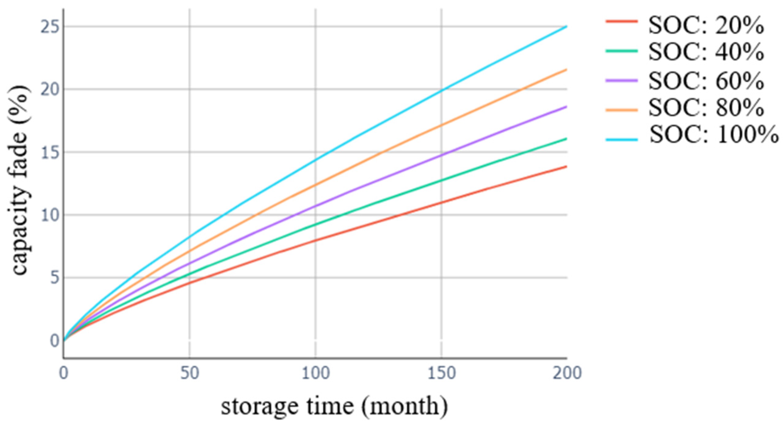
According to the study in [13], under 25 degrees Celsius, the capacity fade can be described in Equation (1).
where represents the percentage of capacity fade, refers to the storage SOC level, and represents the storage period (month).
Figure 5 shows the calendar aging curve drawn by Equation (1). From this figure, it can be seen that the curve is nonlinear and tends to be flat as the storage time increases. In other words, the higher the storage SOC level is, the faster the aging rate will be.
3.3. Cycling Aging
Cyclic aging refers to the aging caused by the charging and discharging cycle of the battery, and its aging performance has a great relationship with cycle depth (CD). Cycle depth indicates the change in charge state during a cycle and is related to the amount of charge gained or lost during the charge and discharge process.
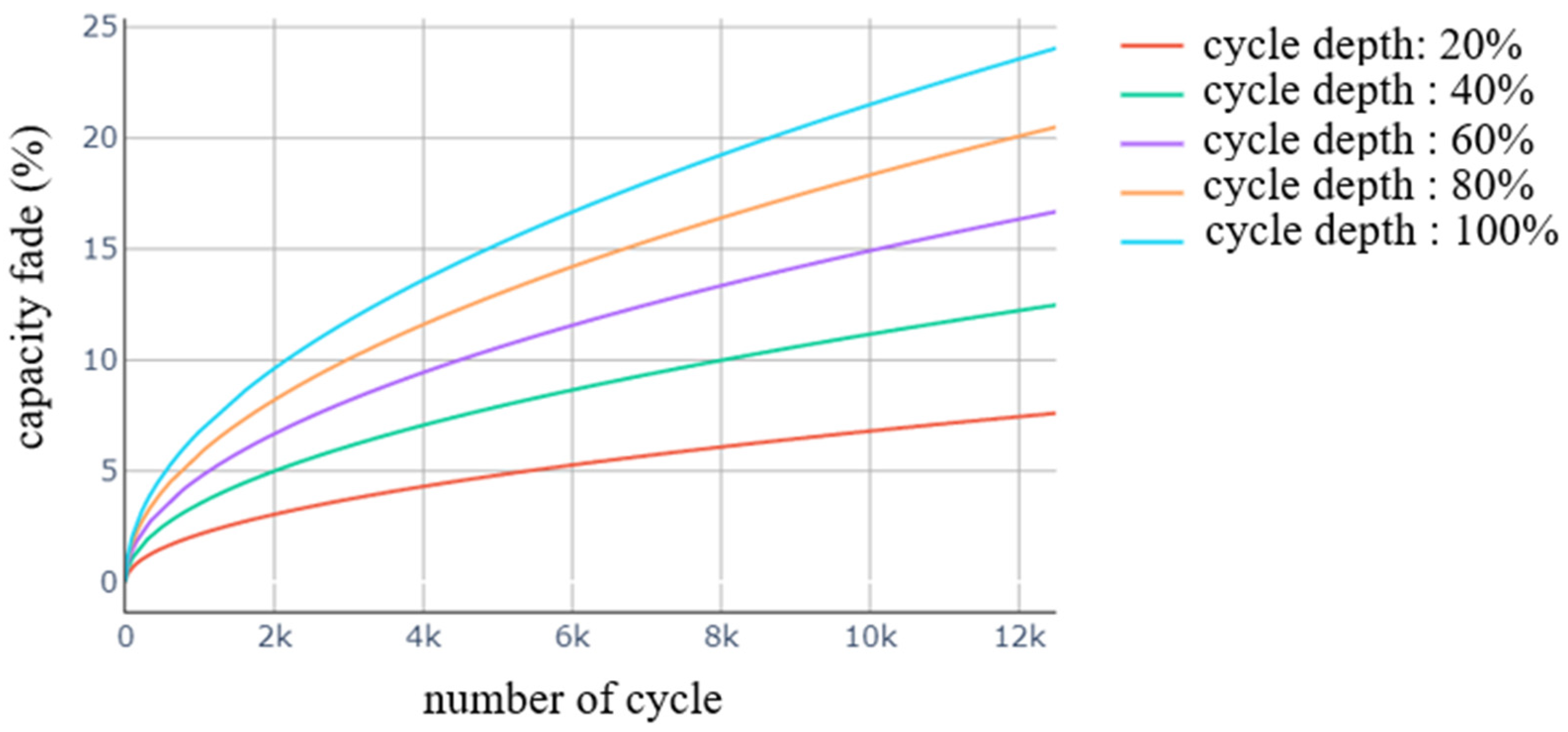
Based on the research in [13], the relationship between capacity fade and the operation conditions, including cycle depth, average SOC, and the number of cycles (NC), under the conditions of 25 °C storage temperature, is shown in Equation (2):
where represents the percentage of capacity fade caused by cycling aging, represents the average SOC level during the cycle, and and represent the cycle depth and the number of cycles, respectively. Figure 6 shows the calendar aging curve drawn by Equation (2).
Compared with calendar aging, the rising slope of cycle aging curve is steeper when the number of cycles is low but tends to be flat when the number of cycles increases. In some cases, the batteries with a deeper cycle depth will have a faster aging rate than the ones with a shallower cycle depth. Sometimes, the difference can be several-fold.
4. Aging Model Establishment
4.1. Introduction of the Aging Model
Since the aging of a battery is a nonlinear problem, it is difficult to apply the traditional mathematical programming method. This research proposes the use of the rain flow algorithm, which has been widely used in the technical and economic analysis of BESS [2,14,15] to solve this nonlinear problem. It extracts the aging features from SOC curves. For details, please refer to Section 4.2.
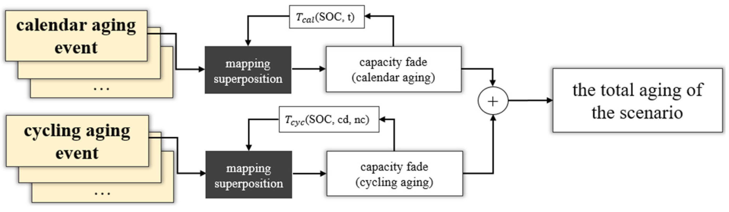
The aging model of lithium-ion batteries in this study can be roughly divided into two parts: the extraction of aging features and the superposition of aging quantity.
In cycle aging, the feature values of each cycle, such as cycle depth, cycle average SOC, and cycle times, were extracted and recorded as cycle aging events. Meanwhile, in calendar aging, the continuous SOC and its duration were recorded as calendar aging events.
The behavior of battery aging has a lot to do with the current aging state of the batteries; thus, even if the operating conditions remain the same, different aging results will be obtained corresponding to the state of aging. Therefore, it is vital to arrange the aging event sequence in the correct order.
After the extraction, the aging features should be quantified and superpositioned. Seeing that the result from each aging event can not be superpositioned directly because the aging curves are not linear, this study proposed a method named the mapping superposition method to solve the problem.
4.2. The Rainflow Cycle Counting Method
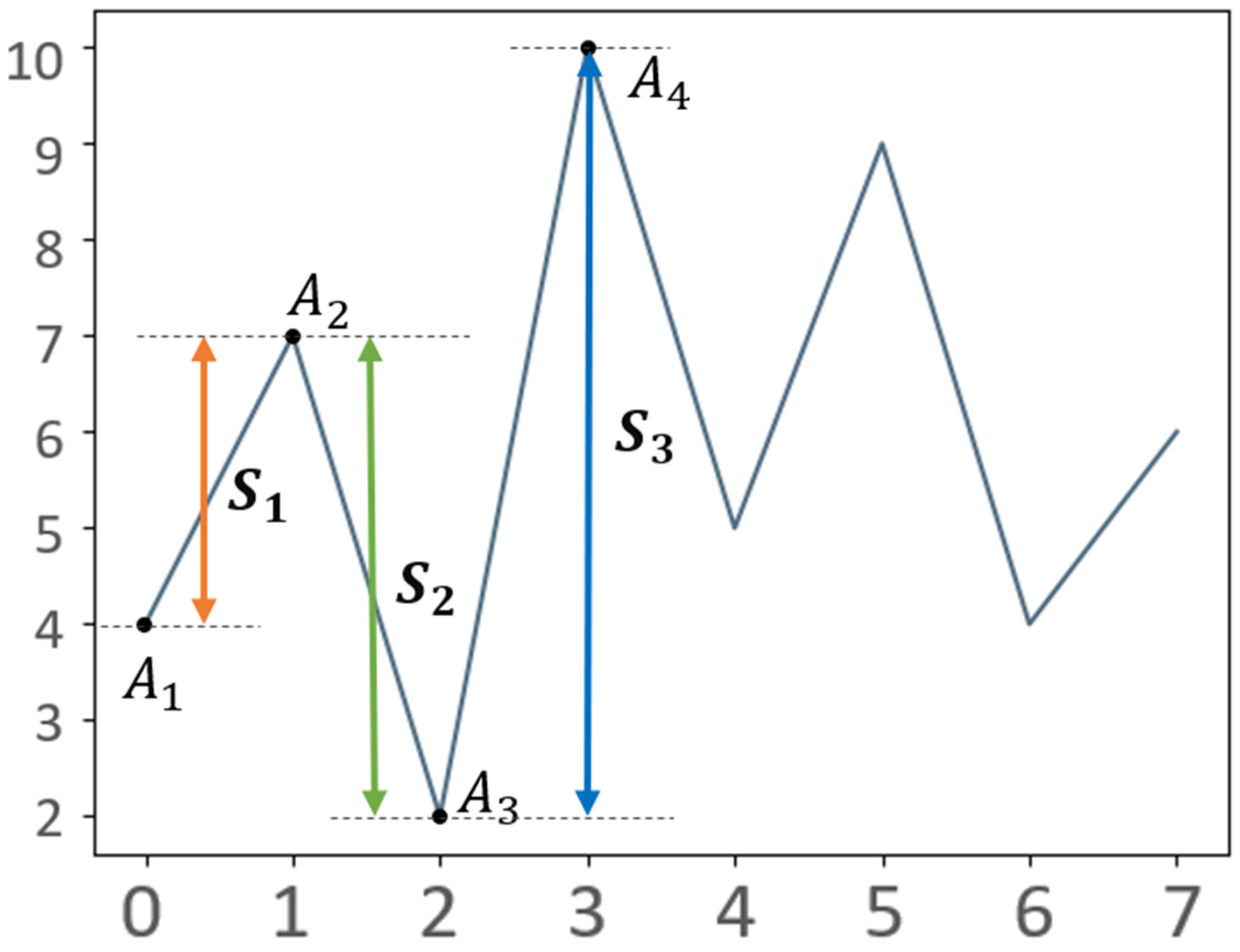
In this study, the four-point algorithm [16] of the rainflow counting method [17] was applied to extract the cycle depth and cycle times.
In the beginning, four consecutive points in the series must be identified and specified as , , , and .Then, calculate the distances , , and between every two adjacent points. The schematic is shown in Figure 7.
If it meets the condition:
then A2 and A3 will be extracted from the series.
Then, the following four adjacent points will be repositioned, operating again until there are no more adjacent four points in the series that meet the conditions. Finally, the remaining sequence will be copied and attached to the end of itself, and then repeated. Examples are described in Appendix A.
4.3. Aging Features’ Extraction
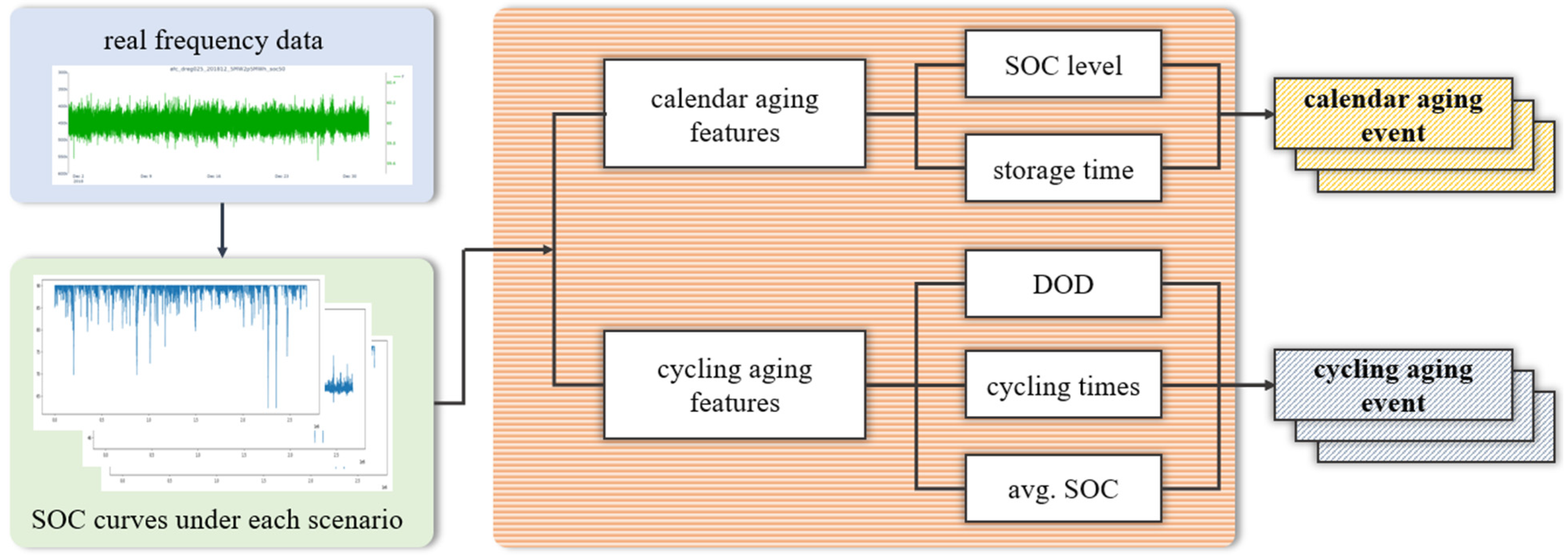
Before the calculation, aging features must be extracted. Figure 8 shows the schematic diagram of the extraction architecture.
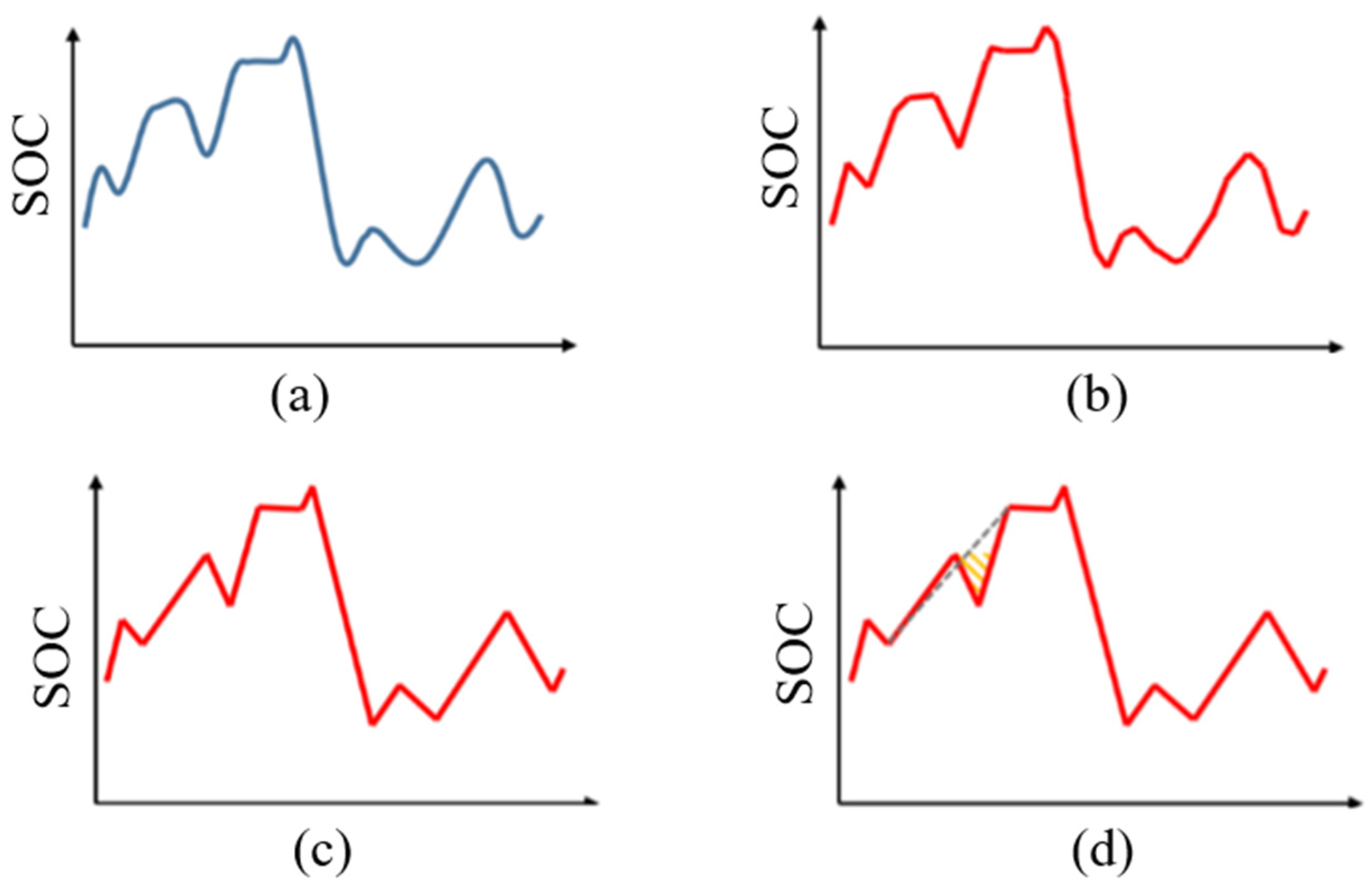
According to the concept of the rainflow counting method mentioned in [18], the continuous SOC curve is processed to remove unnecessary values, leaving only the relative peaks and relative valleys in the series. Therefore, the original SOC curve is filtered twice, and then the rainflow counting algorithm is used. The schematic is shown in Figure 9.
The original input SOC data has a resolution of 0.5%. Through the first filtering, we can separate the continuous parts of the SOC value from the original SOC sequence and record it as calendar aging events, including the placing time and storage SOC. Since the values between the relative maximums and relative minimums are not meaningful during the rainflow cycle counting method, these values should be removed from the sequence first in the following second filtering to generate a new one with only the relative maximums and minimums. In the final stage, cycling aging features such as cycle depth, the number of cycles, and the average SOC of the cycle will be identified through the rainflow counting algorithm and recorded as cycling aging events in sequence.
4.4. Superposition
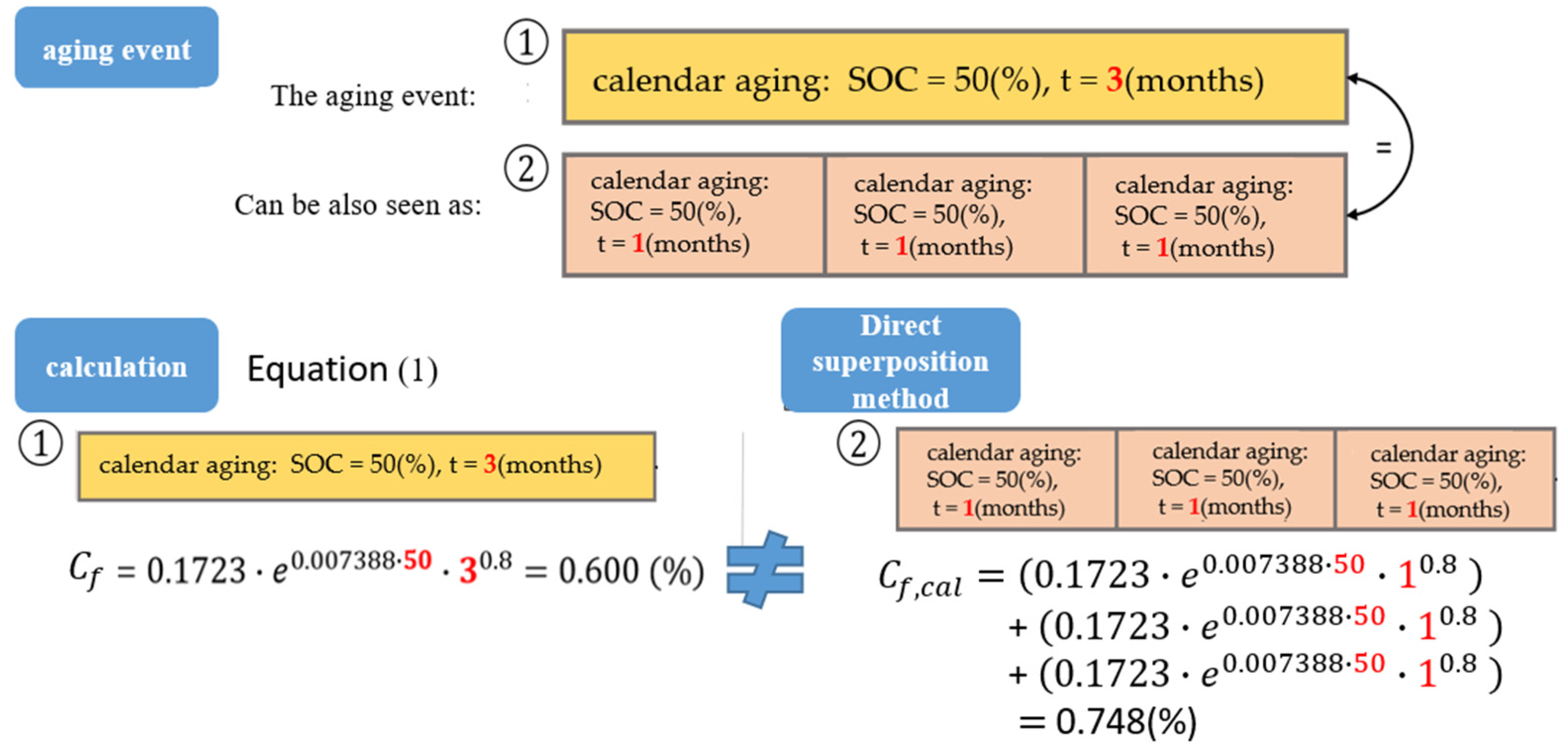
Because the aging behavior of batteries is nonlinear and is affected by more than one variable, the capacity decay caused by aging cannot be superposed directly. Such as the example shown in Figure 10, we can regard the aging event that “maintains the SOC-level at 50% for three months” as three identical continuous aging events that “maintains the SOC-level at 50% for one month”. If we apply the direct superposition method on the latter, which means to superpose the capacity decay by directly adding them together, we will obtain a result that has a considerable disparity from the result of the former.
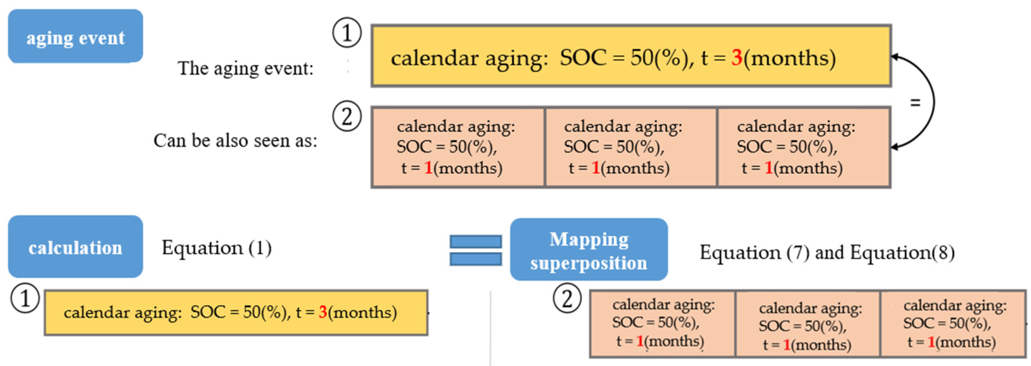
Seeing the incompleteness of the direct superposition method, another method, named the mapping superposition method, is proposed in this study, as shown in Figure 11. In other words, before the superposition, the equivalent quantity of aging features should be calculated according to its former state of the amount capacity fade.
In calendar aging, the former decay quantity must be “mapped” to the curve corresponding to the SOC level of the aging event to be superposed, so as to obtain the equivalent placing time. The equivalent placing time plus the placing time of this aging event is the equivalent total placing time, which can be used to calculate the aging quantity further.
The relevant calculation formula can be derived from Equation (1):
In Equation (7), represents the equivalent placing time, represents the former calendar aging amount, and represents the storage SOC level of this aging event. According to this formula, the equivalent placing time under the conditions of the aging event can be derived. Meanwhile, in Equation (8), and represent the final calendar aging capacity fade after superposing and the placing time in the aging event, respectively.
On the other hand, in the case of cycling aging, the former aging amount should be “mapped” to the curve corresponding to the conditions including cycle depth and the average SOC of the aging event to be superposed, so that the equivalent number of cycles can be derived. The equivalent number of cycles plus the number of cycles of this aging event is the equivalent total number of cycles, which can be used to calculate the aging amount further.
Similarly, in Equation (9), , , , and represent the equivalent number of cycles, the former cycling aging amount, the cycle depth, and the average SOC of this aging event, respectively. In Equation (10), stands for the capacity fade after superposing, while refers to the number of cycles of the aging event.
Applying the mapping superposition method, a result closer to the theoretical values than that when using the direct superposition method can be obtained, as shown in Figure 12.
5. Result of Simulation
5.1. Simulation Scenario
Under the same frequency, different frequency regulation modes will have their required output so that their corresponding SOC curves can be generated. Then, the different aging features can be extracted and recorded from each by implementing the aging model.
Based on the aging results of dReg0.25, dReg0.5, and sReg under different BESS system parameters, including the rated power and the storage capacity, this study will iterate them repeatedly in three months until the capacity fade reaches 20%, i.e., the end-of-life (EOL) criteria. This paper uses SOC curves under nine different scenarios of different modes and different BESS system parameters to simulate the aging results, then discuss the performances of each. Table 2 shows each scenarios.The real frequency data of Taiwan in three different seasons, December 2019, March 2020, and May 2020, were used as input data for every scenario. The frequency distribution and features of the SOC curves are described in Appendix B.
5.2. Result and Discussion of Each Scenario
This section compares the battery aging results under each scenario, discussing the relationship between the capacity fade behavior and the system conditions, including the frequency regulation service mode, the rated power, and the storage capacity. Table 3 shows the detailed information of the comparisons.
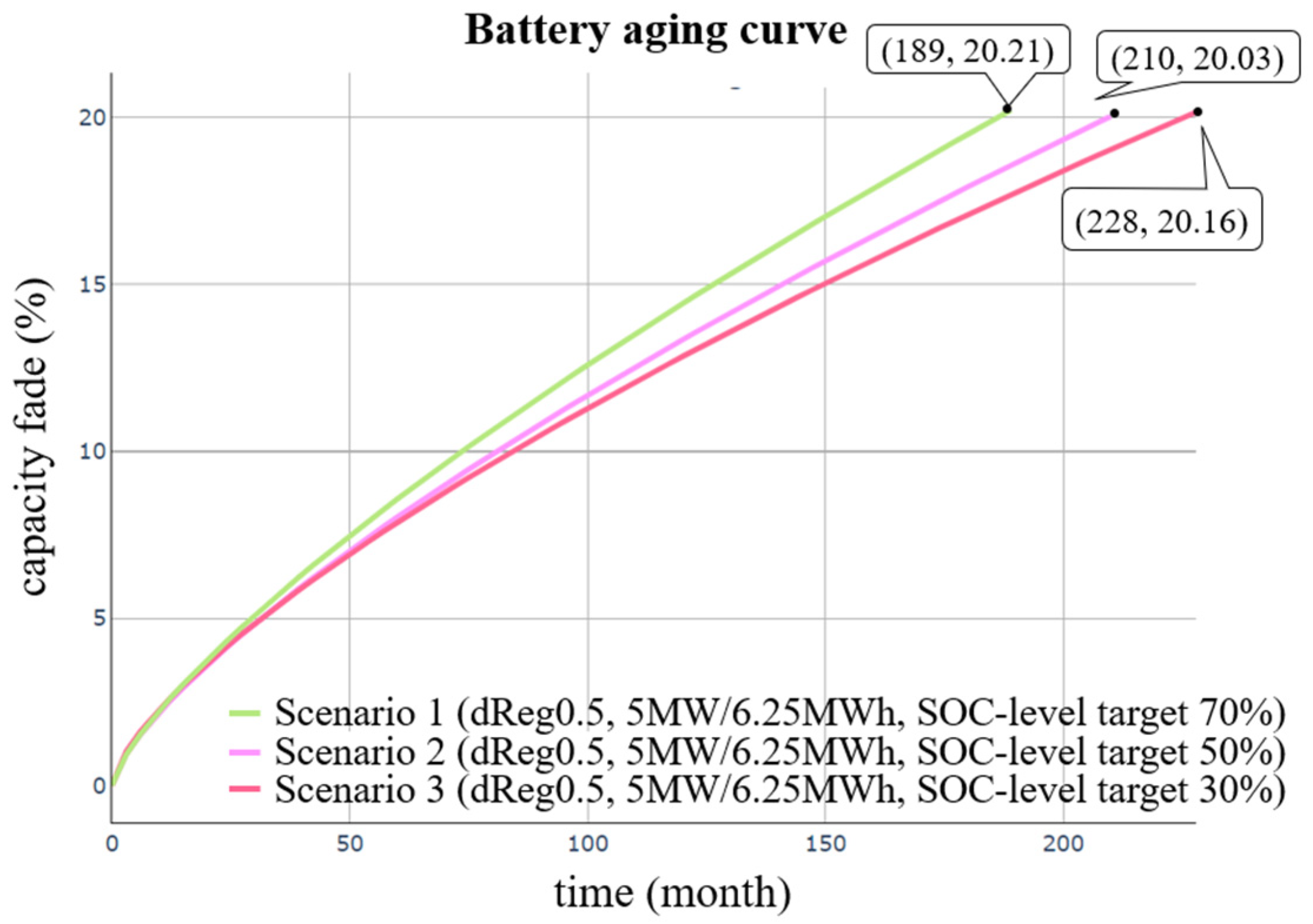
- dReg0.5 with the same rated capacity and battery energy but a different SOC level target:
Scenario 1, 2, and 3 were all in dReg0.5 mode with a 5 MW/6.25 MWh BESS. The only difference was the SOC level targets, with 70%, 50%, and 30%, respectively. As shown in Figure 13, Scenario 1, the one that had the highest SOC level target had the shortest lifetime, as described in Section 3.2.
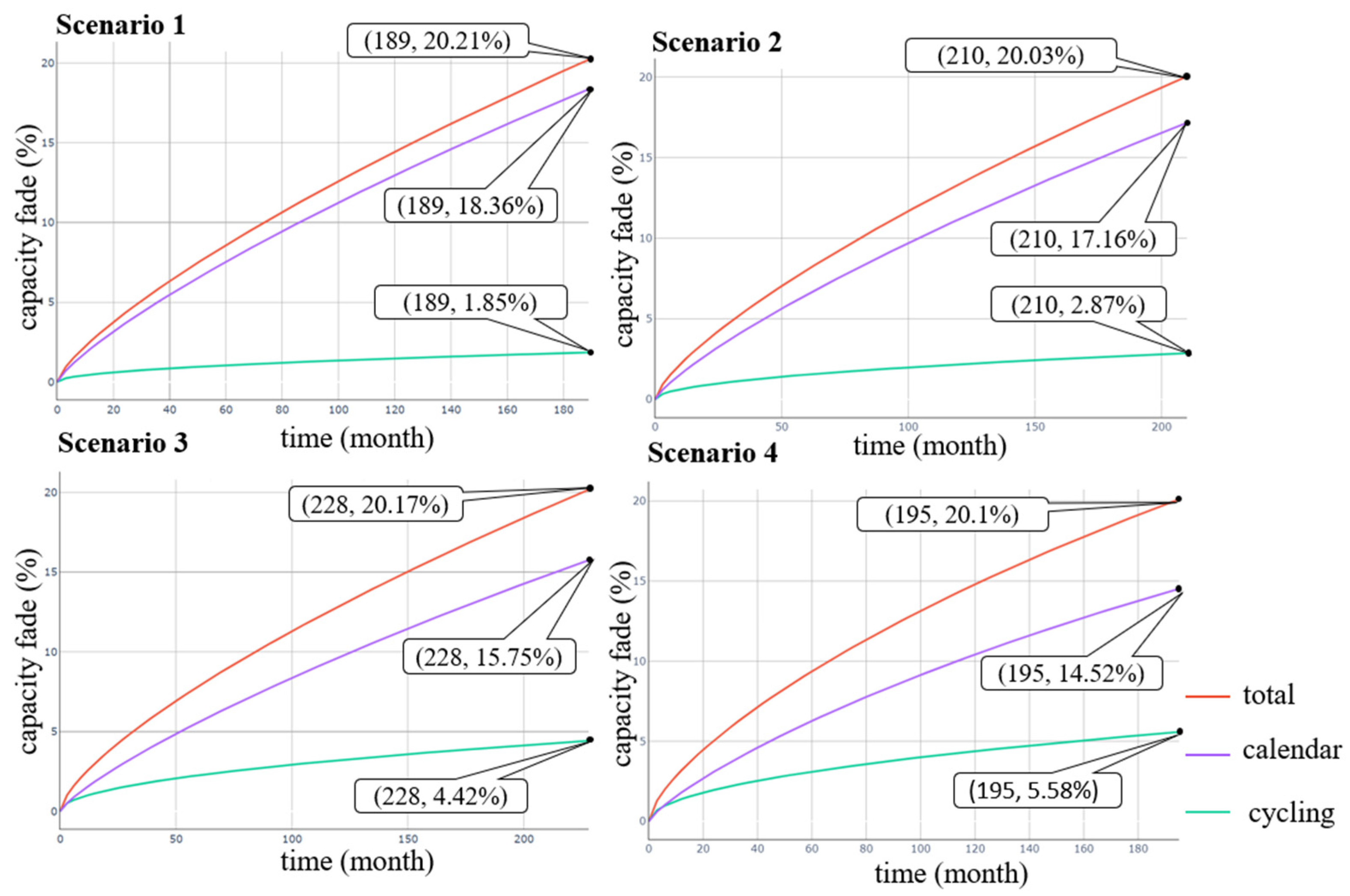
Calendar aging was the main source of capacity fade of the three scenarios, as shown in Figure 14. Since the SOC level target of Scenario 1 was the highest, its capacity fade caused by calendar aging was the highest among the three. Calendar aging was continuously accumulating, so the higher the calendar aging rate, the shorter the life it had. This was probably the reason why Scenario 1 reached its end-of-life the earliest. Maintaining the SOC at 30% yielded 8.5% more lifetimes than 50%, 20.6% more lifetimes than 70%.
- B.
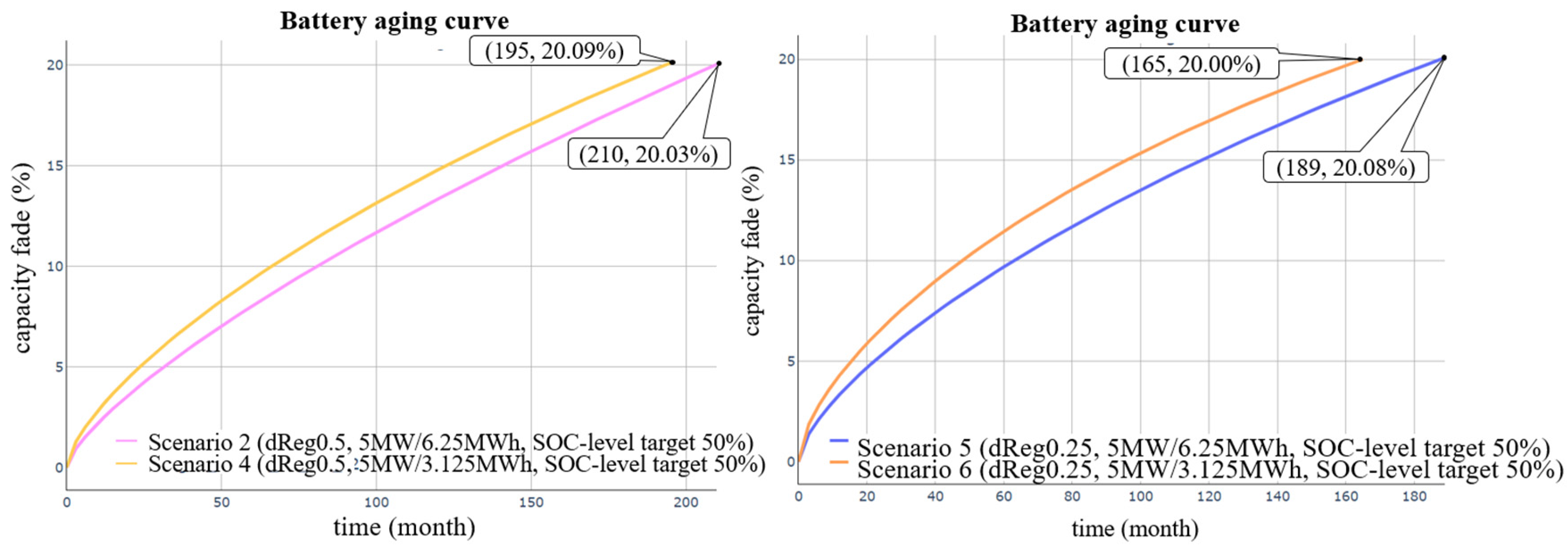
- dReg with the same rated capacity but a different battery energy:
Both Scenarios 2 and 4 used the dReg0.5 mode with the same rated power of 5 MW but had different storage energies of 6.25 and 3.125 MWh, respectively, with the results shown in Figure 15. Similarly, both Scenarios 5 and 6 used the dReg0.25 mode but also differed in the storage energy.
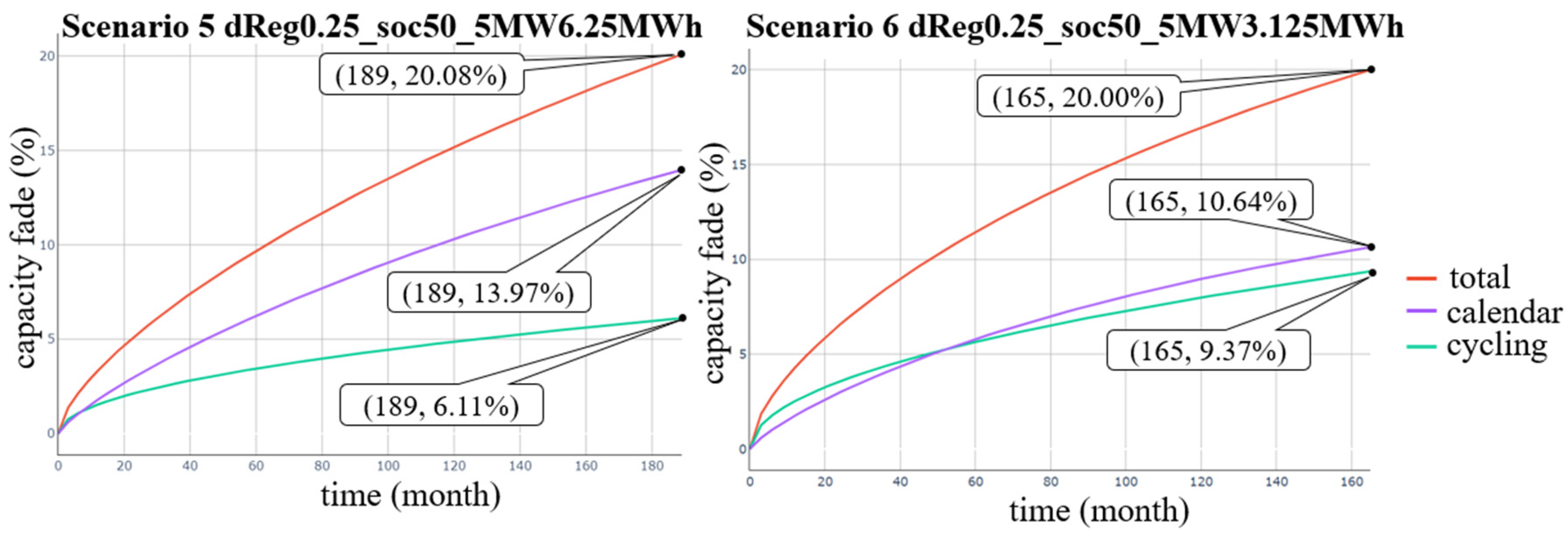
As shown in Figure 16, although most of the aging in the four different situations came from calendar aging, the fade caused by cycling aging in Scenario 4 was significantly higher than that in Scenario 2, and in Scenario 6 it was also higher than that in Scenario 5. Since the SOC level target was 50% for each scenario in this comparison, theoretically, the rate of calendar aging should not have been significantly different. Therefore, it was estimated that with the same SOC level target, the cycle times and depth of the scenario with a higher C-rate would be more than that of the one with a lower C-rate, and thus, it would reach EOL faster.
- C.
- dReg0.5 and dReg0.25 with the same rated capacity and battery energy:
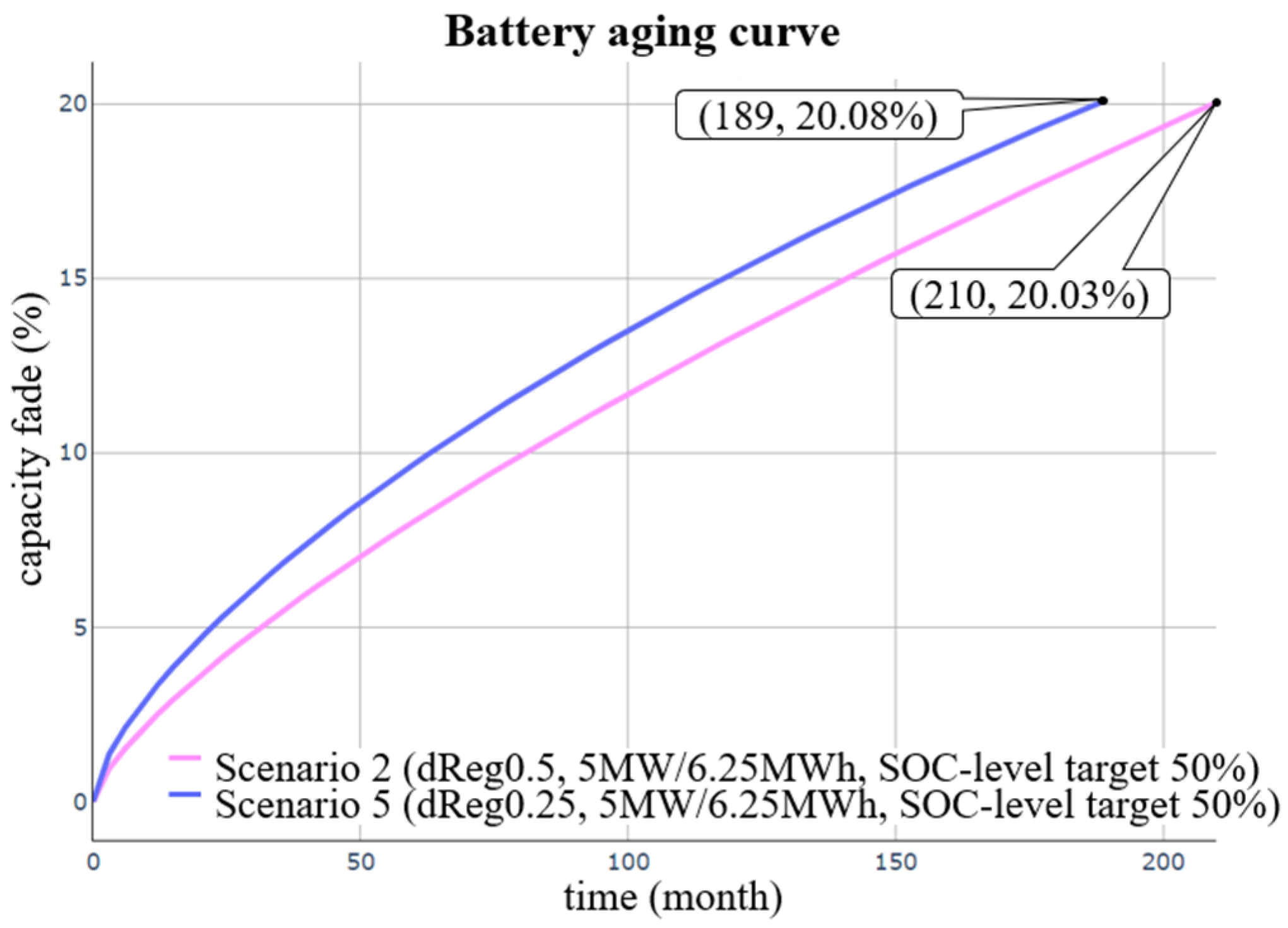
Scenario 2 and Scenario 5 were dReg0.5 and dReg0.25 at 5 MW/6.25 MWh, respectively, with the results shown in Figure 17. In this case, it can be estimated that for the energy storage system with the same rated capacity and the same total battery energy, the battery lifetime of dReg0.5 mode would be longer than that of dReg0.25.
Compared with dReg0.5, dReg0.25 often needs to carry out more output outside the deadband, so the cycle depth of dReg0.25 is higher than that of dReg0.5 under the same frequency conditions. Therefore, the capacity fade rate caused by cycling aging of dReg0.25 is much faster than that of dReg0.5, which indirectly leads to dReg0.25 reaching the end of battery life faster.
- D.
- sReg with the same rated capacity and SOC level target but different battery energy:
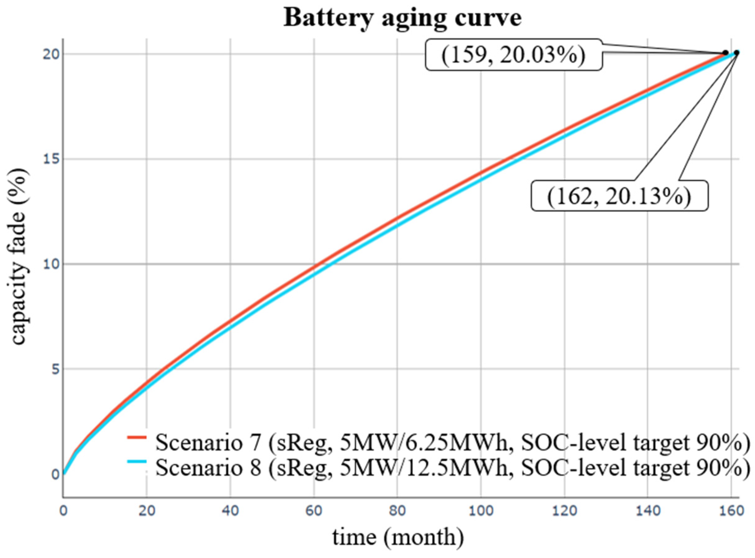
As shown in Figure 18, Scenario 8 with a lower C-rate did lived longer than with a higher C-rate (Scenario 7), but the difference was almost negligible. Considering the cost of installation, the total battery energy of Scenario 8 was twice that of Scenario 7, which may not be economical.
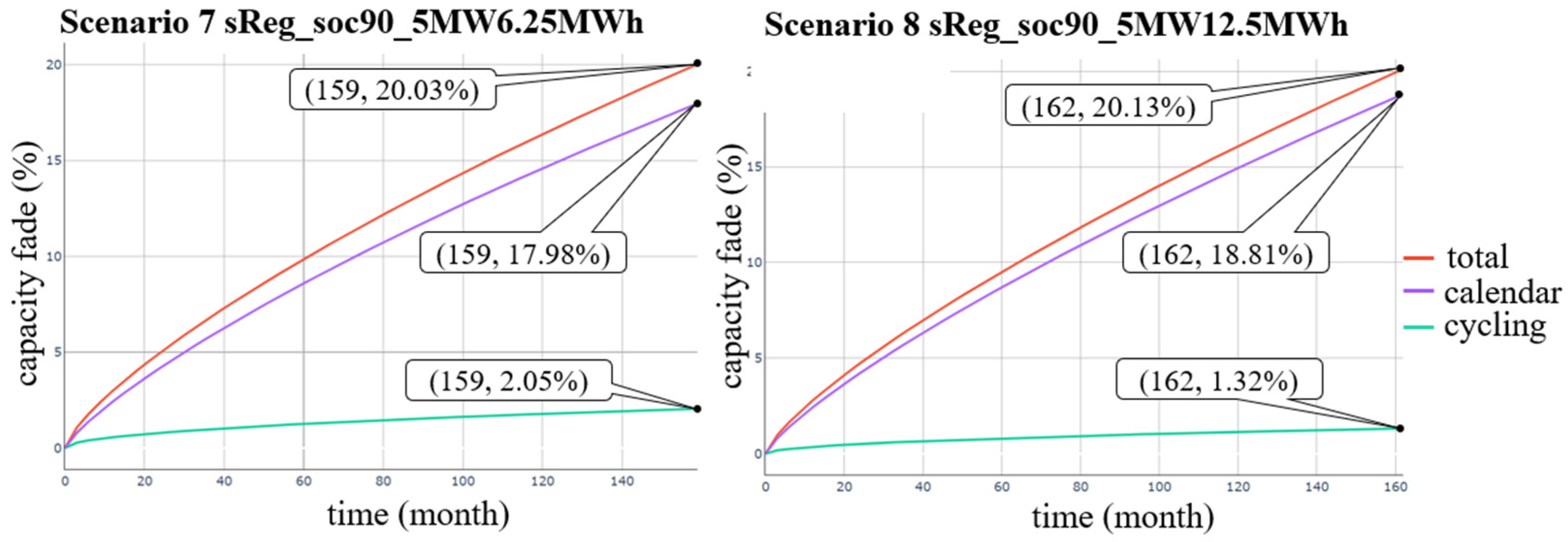
As shown in Figure 19, in the scenarios of the sReg mode with the SOC level target at 90%, the proportion of calendar aging was significantly higher than that of cycle aging, especially in the case of Scenario 8, which almost dominated the battery life. Outputting the same power, the SOC variation of the scenario with a lower C-rate will be lower than that of the one with a higher C-rate, so in the long run, the overall capacity fade caused by cycling aging will indeed be lower. However, as the proportion of cycling aging in these scenarios was not high, the effect of reduced cycle aging on the overall battery life was not significant.
- E.
- sReg with the same rated capacity and battery energy but different SOC level target:
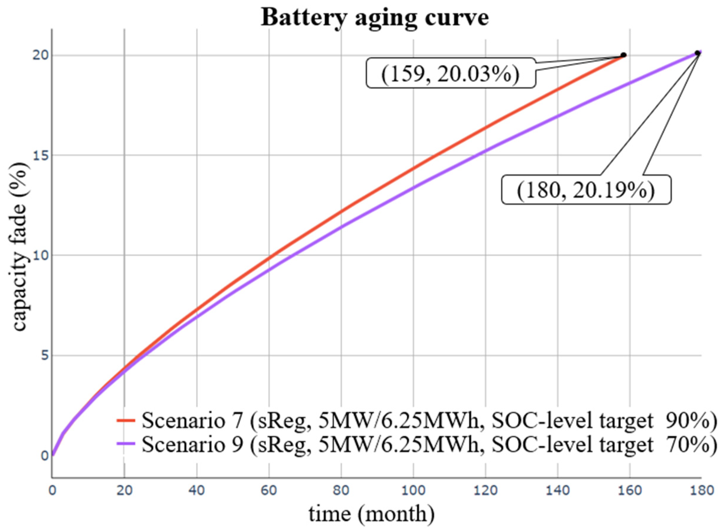
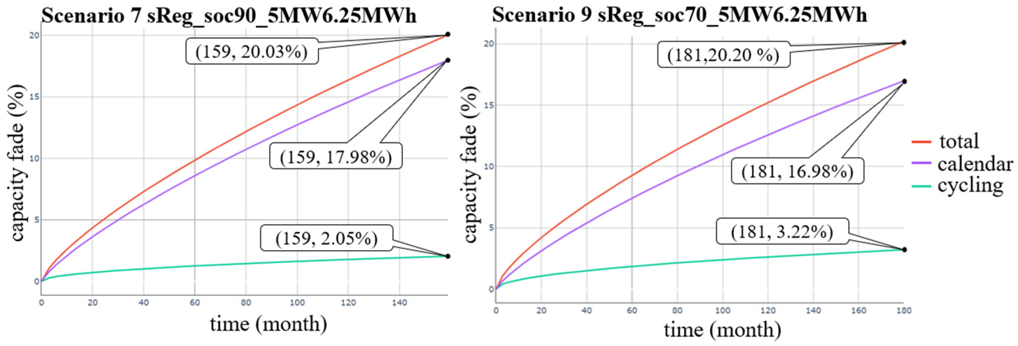
As shown in Figure 20, Scenario 7, which had a SOC level target of 90%, reached its end-of-life after only 159 months, while Scenario 9, with a 70% SOC level target, reached EOL through 180 months of use. In conclusion, it could be preliminarily supposed that those with a lower SOC level target had a longer battery life.
As shown in Figure 21, in Scenario 7, because the SOC level target was higher than that of Scenario 9, the calendar aging rate was higher, which made it reach the end-of-life faster. Simply by lowering the SOC level target, the battery life of Scenario 9 would be about 20 months longer than that of Scenario 7. Therefore, if the SOC level target could be as low as possible within the allowable range, the battery could have a longer lifetime.
Table 4 shows the battery life of all the scenarios. From (Scenario 1, 2, 3), (Scenario 7, 9) it was found that lowering the SOC level significantly improved battery life. From (Scenario 3, 4), (Scenario 5, 6), and (Scenario 7, 8) it was found that the battery life with a lower capacity was shorter.
5.3. Profit Estimation and Comparison
Table 5 is a rough estimate of the system construction costs based on the statistics of the data from various manufacturers [19]. , , and represent the cost of the storage block (SB), storage-balance of system (SBOS), and power equipment (PE), while and stand for the rated power and battery energy, and finally, refers to the cost of the entire BESS.
This study calculated the profit earned until EOL in each situation, and the related formulas are shown in Equations (11) and (12). To simplify the calculation, there were some simple assumptions in this paper:
where and represent the total revenue and net profit estimated until the battery’s EOL; represents the number of months until the battery reaches its EOL. , , and represent the capacity offer price described in Table 1, the efficiency offer price varying with the market bidding price every day, and the quality factor of operation, respectively.
- dReg0.5 with the same rated capacity and battery energy but different SOC level target:
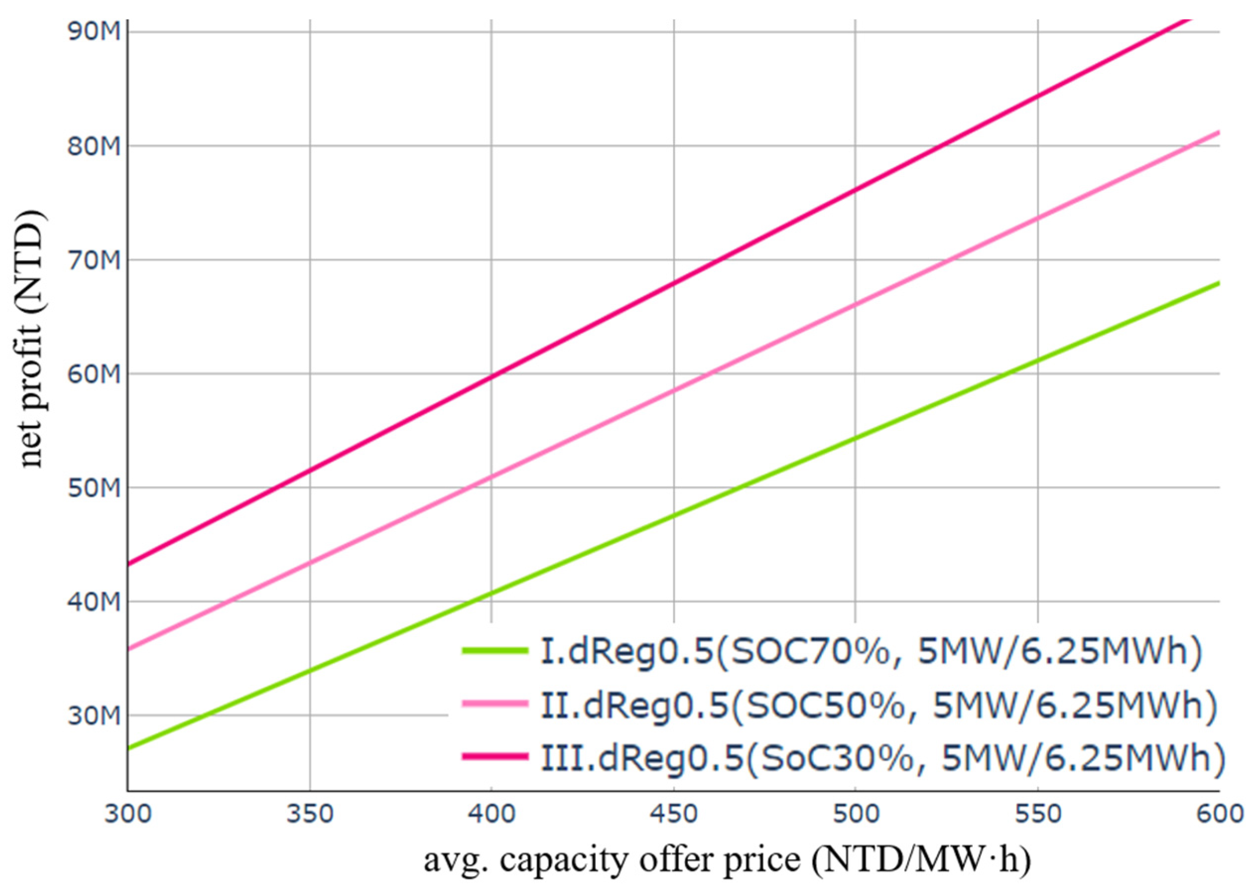
As shown in Figure 22, Scenario 3 had the highest net profit among the three. The BESS specifications of the three Scenarios were the same so that the construction cost was also the same. Scenario 3 had the longest battery life and could thus earn the most profit.
- B.
- dReg with the same rated capacity but different battery energy:
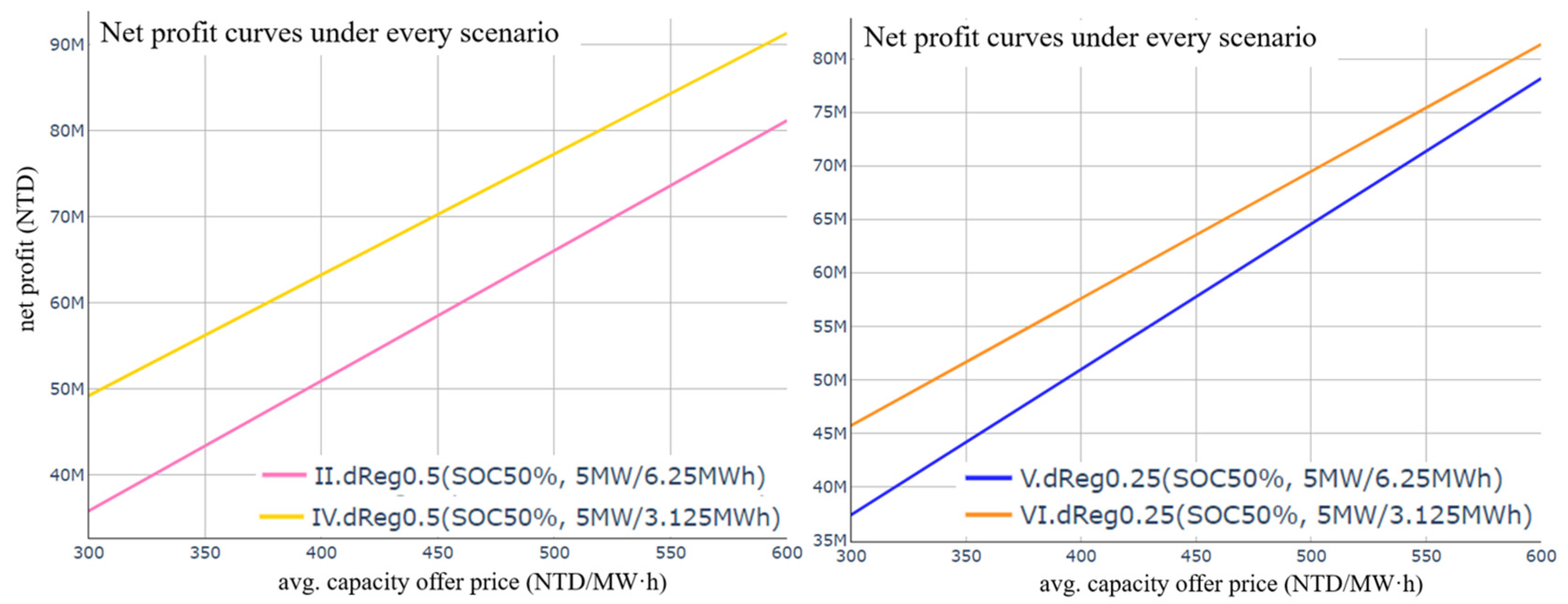
As shown in Figure 23, either under the dReg0.5 or dReg0.25 mode, those with a higher C-rate had a higher net profit in the simulation results of this study. Although the battery life of those with a higher C-rate was shorter, the construction cost of their BESS was lower. Therefore, the net profit was still higher than that of those with a lower C-rate. However, these results are only the conclusion from the simulated data in this study; thus, the real results may vary due to the actual construction cost of actual sites and many other factors.
- C.
- dReg0.5 and dReg0.25 with the same rated capacity and battery energy:
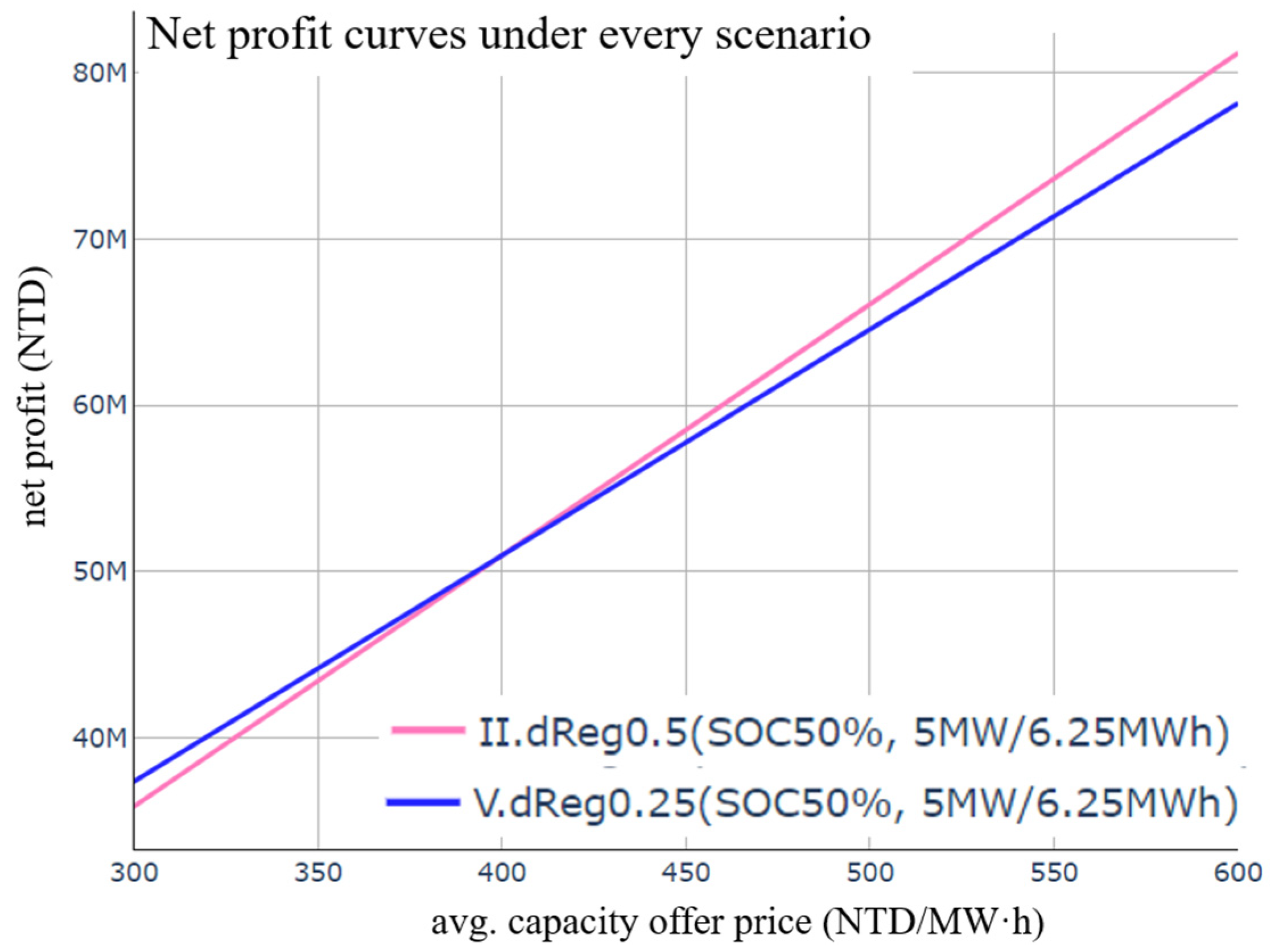
As shown in Figure 24, the net profit difference between Scenario 2 and Scenario 5 was small. The two scenarios had the same specifications of BESS, so the construction cost was similar, but dReg0.5 (Scenario 2) had a slightly longer life. dReg0.5 and dReg0.25 have different efficiency offer prices, which is one of the main factors that determine the profits; thus, in this case, the one that had a longer battery life did not necessarily give more net profit.
- D.
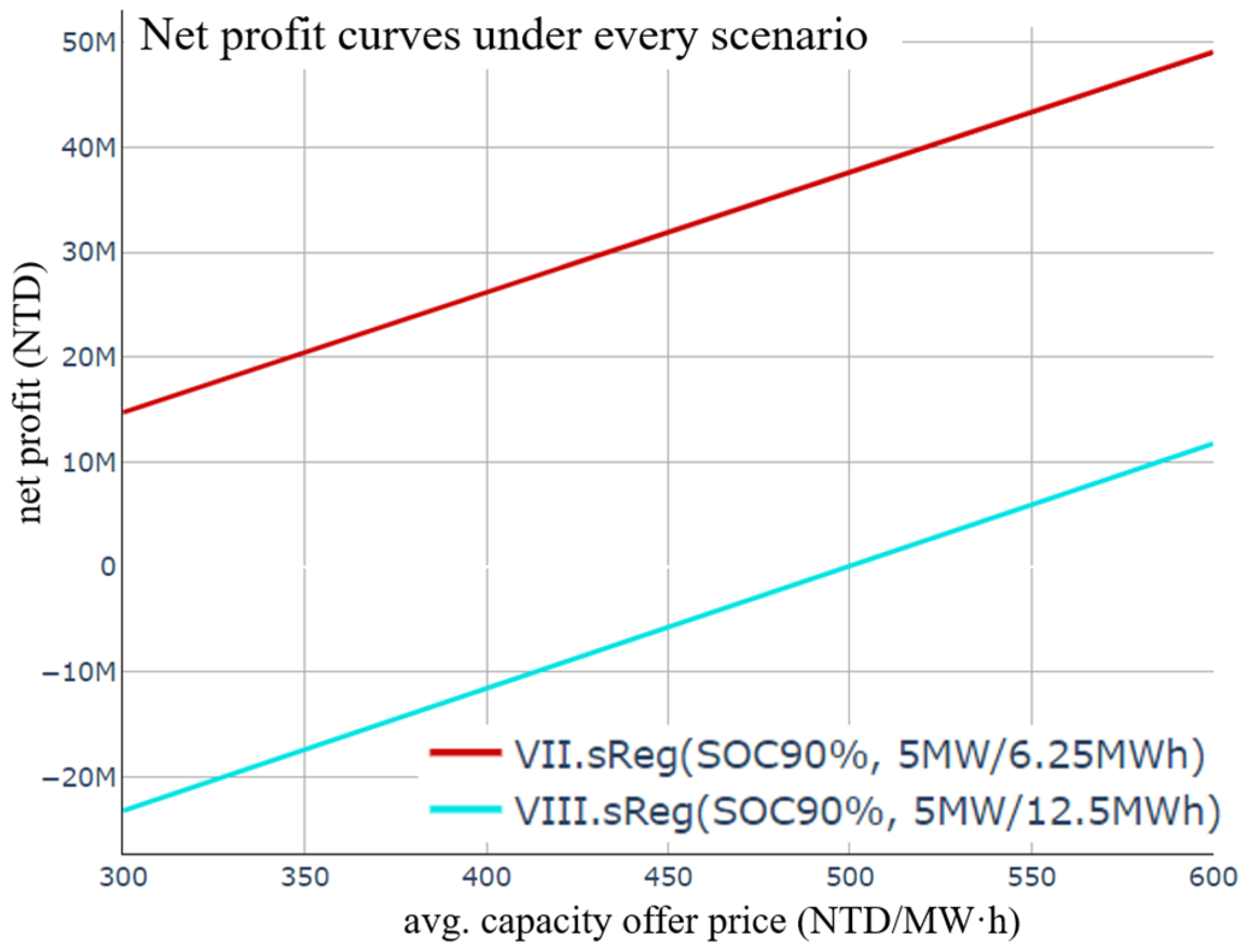
- sReg with the same rated capacity and SOC level target but different battery energy:
As shown in Figure 25, the battery life in Scenario 8 was slightly longer than that in Scenario 7, but the difference was almost ignorable, so the total revenue should have been about the same. Since the construction cost of Scenario 8 was significantly higher than that of Scenario 7, the former had a dramatically lower net revenue than the latter.
- E.
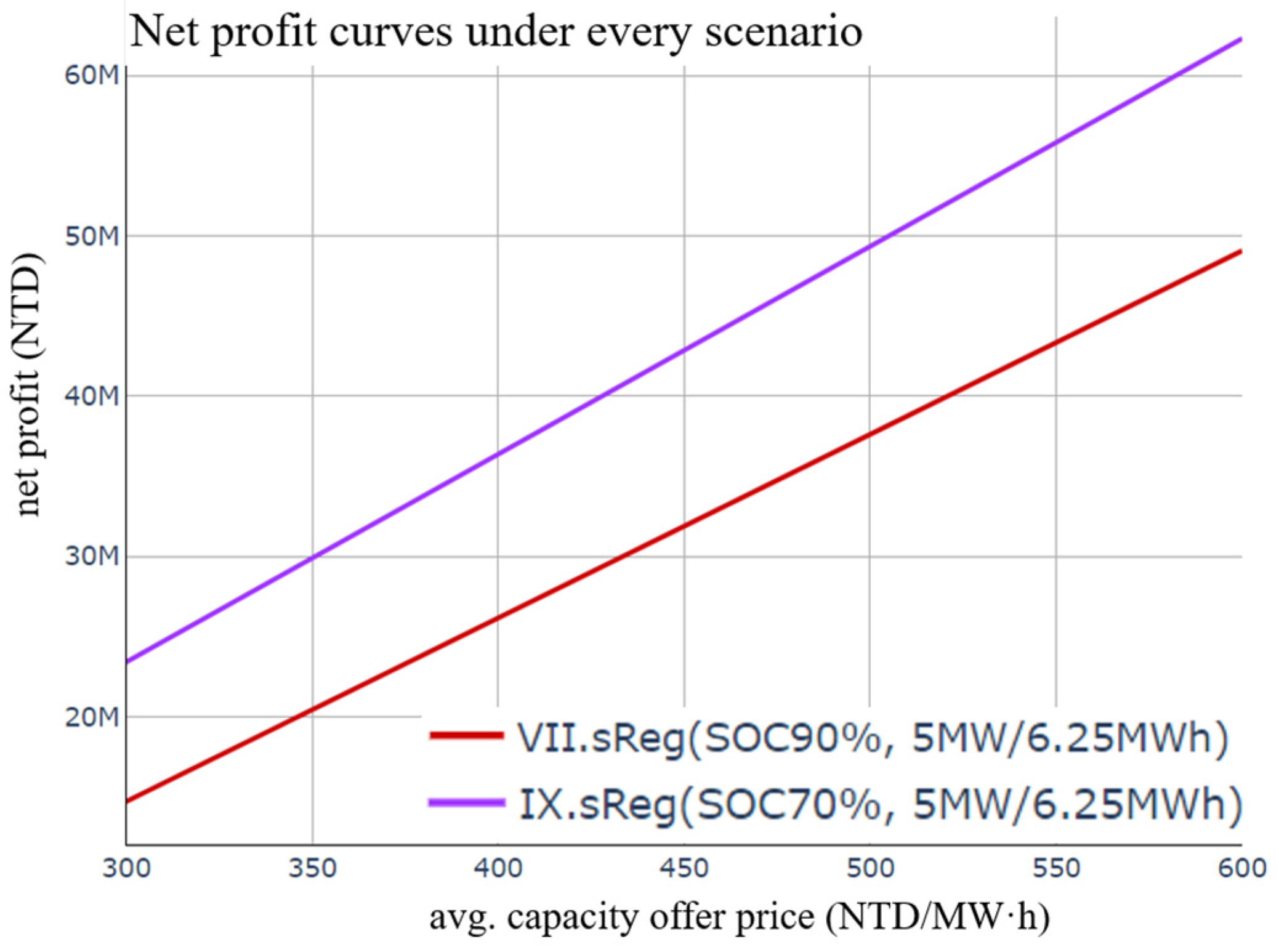
- sReg with the same rated capacity and battery energy but different SOC level target:
Figure 26 shows that a lower SOC level target led to a higher net profit because of its longer battery life; thus, Scenario 9 had a higher net profit than Scenario 7 did.
For the results of this study, considering the operational requirements of dReg0.5 and dReg0.25 modes, it was not necessary to maintain SOC at a high level. On the contrary, a high SOC level target was necessary for the sReg mode to cope with the situation of long-time full-power output.
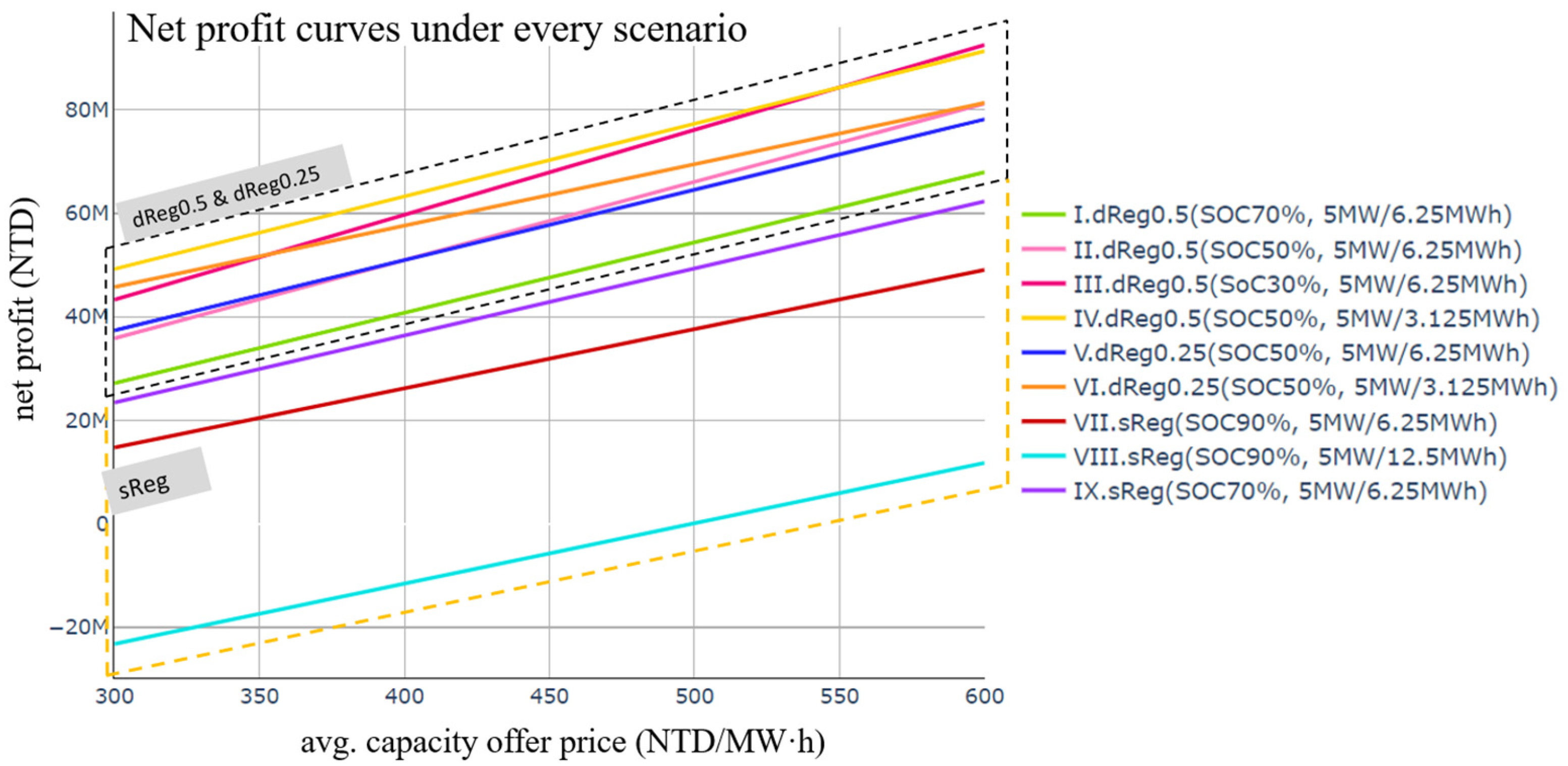
Figure 27 shows the net profit curves of all scenarios. The net profits of the scenarios under dReg0.5 were close to those under dReg0.25, but they were all generally higher than that under sReg.
From this simulation, it was estimated that for either dReg0.5 or dReg0.25 modes, the net profits of those with a higher C-rate would indeed be higher than that of those with a lower C-rate, but the effect did not seem to be that significant. Under the sReg mode, the reduction of C-rate did not bring much benefit to the battery life but led to a significant decrease in net profit due to the increased construction cost. Finally, SOC-level-targeting had a significant impact on overall net profits regardless of what the frequency regulation mode was, so evaluating to which level to set the SOC target is critical to enhancing the profits.
6. Discussion
From (Scenario 1, 2, 3), (Scenario 7, 9) it was be found that a low SOC level gave a higher net profit. Therefore, market participants can increase revenue by reducing the SOC level. From (Scenario 3, 4), (Scenario 5, 6), and (Scenario 7, 8), it was found that no matter how the price changed, the income of a high-C-rate battery was always relatively high and its construction cost was relatively low. It could be inferred that this market is more suitable for high-C-rate batteries. The net profit in Scenario 8 was below zero most of the time, which meant that if the capacity selection is wrong, it may lead to loss of money in the sReg market.
7. Conclusions
This research has shown that there are differences in battery life under different frequency regulation. The following can be observed for each type of frequency regulation:
For systems under dReg0.5, those with a lower SOC level target had a longer battery life and, thus, a higher net profit.
Then, comparing the systems in dReg0.5 and dReg0.25 modes, although the battery life of the system with a lower C-rate was longer, when considering the construction cost, it did not mean that the net profit would be more than that of the system with a higher C-rate.
Finally, for the sReg, since most of the aging comes from calendar aging, the SOC level maintained for a long time seriously affected its battery life. Furthermore, the lower the SOC level, the longer the life. In addition, the effect of a low-C-rate battery on increasing the lifetime was not significant, and the cost was relatively high, so the high C-rate scenario had higher net profit. For a BESS with the same rated power and the same total energy capacity, due to sReg usually being used in response to possible emergencies which needs BESS to maintain a higher SOC level than that in the other two services, it results in a shorter battery life and a lower net income for the batteries operating with sReg.
The limitation of the proposed method is that even for batteries of the same chemical material, batteries manufactured by different battery manufacturers will still have different aging properties, and the parameters of the model need to be adjusted according to different batteries.
Future research will focus on evaluating the optimal capacity configuration of BESS in various ancillary services. Because the BESS of more than hundreds of MW will be composed of dozens of PCS with batteries of a specific capacity, the overall C-rate can be very fine; any number between 0.25–1C is possible, and it is not limited to a specific C-rate. It depends on how many PCS and how many batteries are used. The method proposed in this study can iterate the most suitable configuration according to various regions and various auxiliary services.
Author Contributions
Conceptualization, C.-C.K.; Data curation, C.-H.K.; Funding acquisition, C.-C.K.; Investigation, C.-H.W. and J.-Z.J.; Project administration, C.-H.W. and C.-C.K.; Resources, C.-H.W.; Software, C.-H.K.; Supervision, C.-C.K.; Validation, J.-Z.J.; Visualization, C.-H.K.; Writing—original draft, C.-H.K.; Writing—review & editing, J.-Z.J. All authors have read and agreed to the published version of the manuscript.
Funding
The support of this research by the Ministry of Science and Technology of the Republic of China under Grant No. MOST 111-2622-8-011-006-TE1 is gratefully acknowledged.
Institutional Review Board Statement
Not applicable.
Informed Consent Statement
Not applicable.
Data Availability Statement
All data are provided in this manuscript.
Conflicts of Interest
The authors declare no conflict of interest. The funders had no role in the design of the study; in the collection, analyses, or interpretation of data; in the writing of the manuscript, or in the decision to publish the results.
Appendix A
Figure A1.
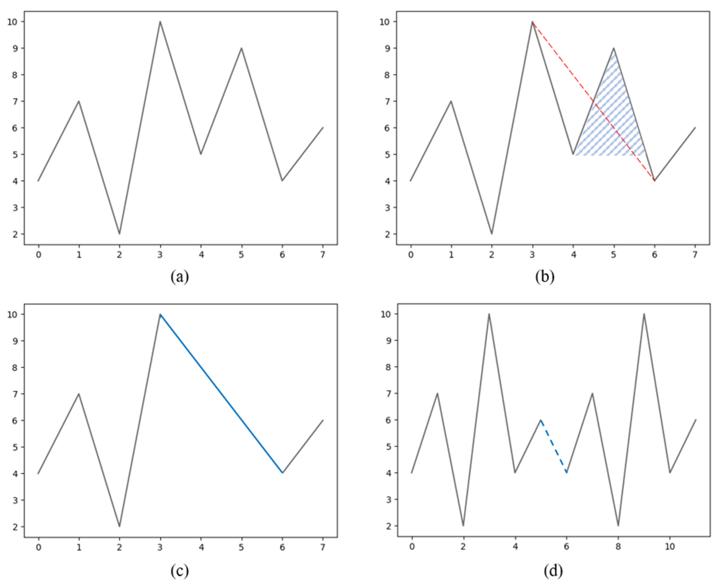
Example of extracting a single cycle using the rainflow counting algorithm. (a) It shows a line graph of the original sequence [4, 7, 2, 10, 5, 9, 4, 6] (b) Using rainflow counting method extract cycle: 5-9, the depth of this cycle is 4, the average is 7. (c) It shows the sequence after the extraction (d) Concatenate the original sequence with other sequences.
Figure A1.
Example of extracting a single cycle using the rainflow counting algorithm. (a) It shows a line graph of the original sequence [4, 7, 2, 10, 5, 9, 4, 6] (b) Using rainflow counting method extract cycle: 5-9, the depth of this cycle is 4, the average is 7. (c) It shows the sequence after the extraction (d) Concatenate the original sequence with other sequences.

Figure A2.
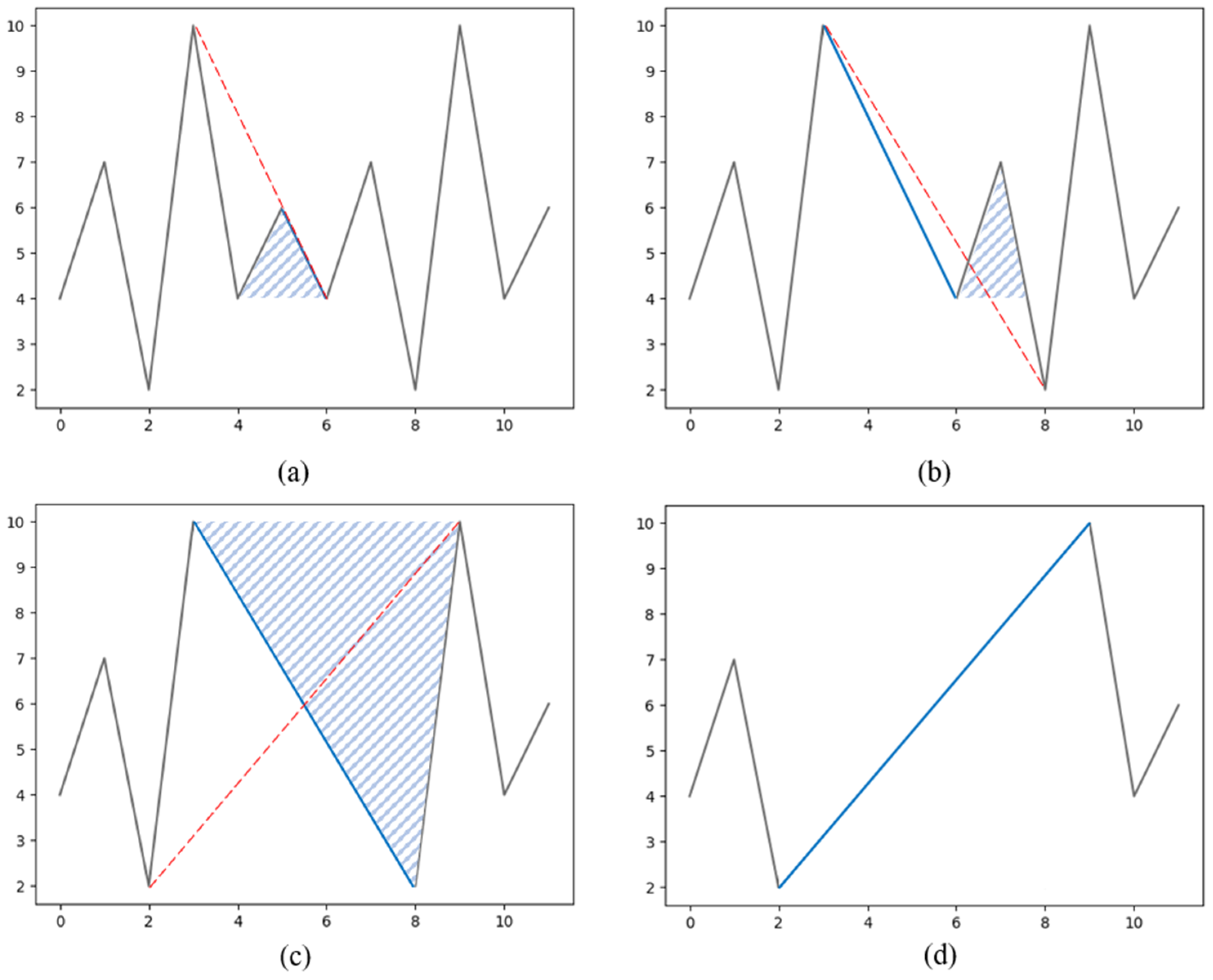
Example of extracting several cycles using the rainflow counting algorithm. (a) Extract the cycle of the blue triangle and use the red dotted line to fill the interval, the cycle depth is 2, the average is 5. (b)Using the same method to extract cycle [4,7], depth is 3, average is 5.5. (c) Use the same method to extract cycle [2,10], depth is 8, average is 6. (d) Sequence after Extraction.
Figure A2.
Example of extracting several cycles using the rainflow counting algorithm. (a) Extract the cycle of the blue triangle and use the red dotted line to fill the interval, the cycle depth is 2, the average is 5. (b)Using the same method to extract cycle [4,7], depth is 3, average is 5.5. (c) Use the same method to extract cycle [2,10], depth is 8, average is 6. (d) Sequence after Extraction.

Appendix B
Figure A3.
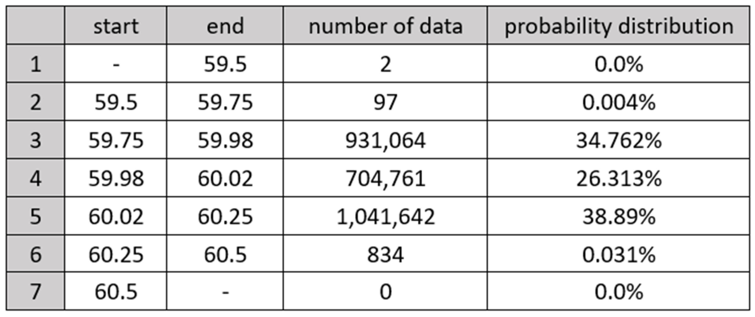
Frequency distribution of December 2019.

Figure A4.
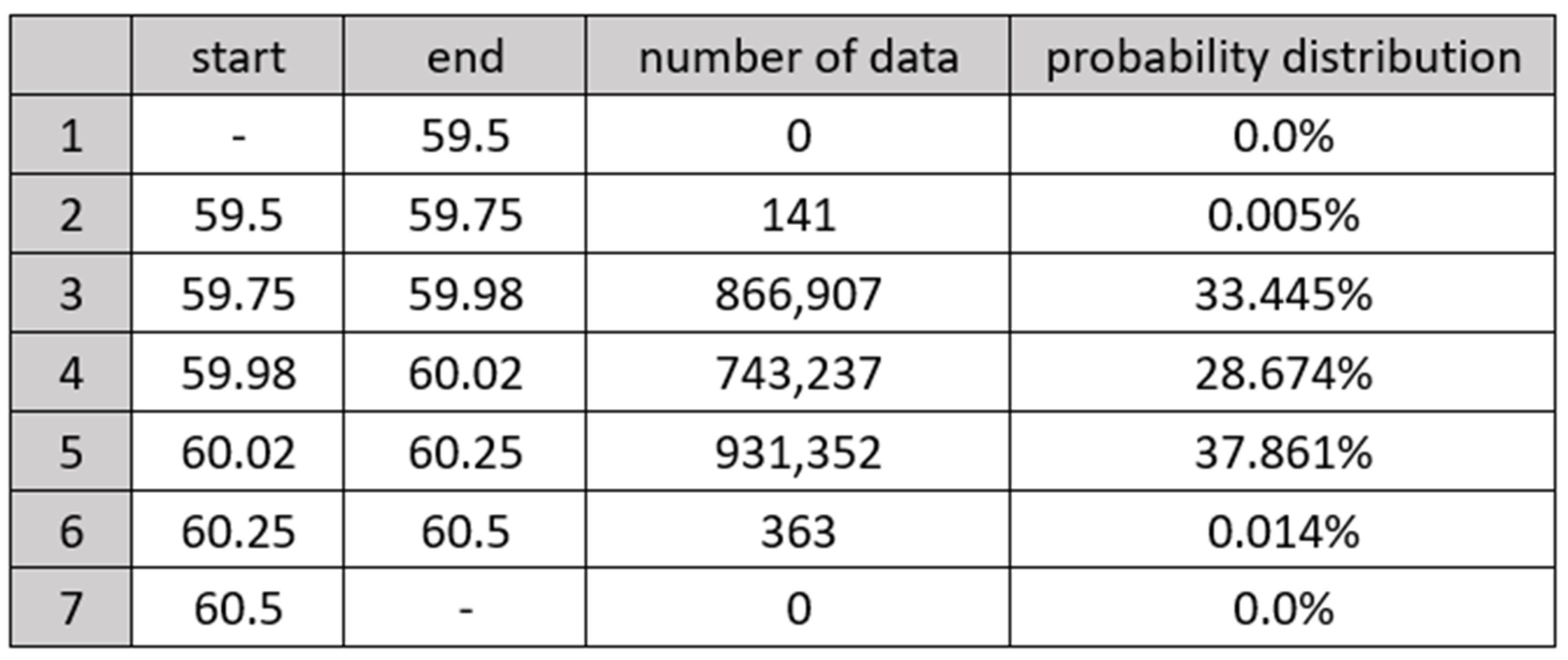
Frequency distribution of March 2020.

Figure A5.
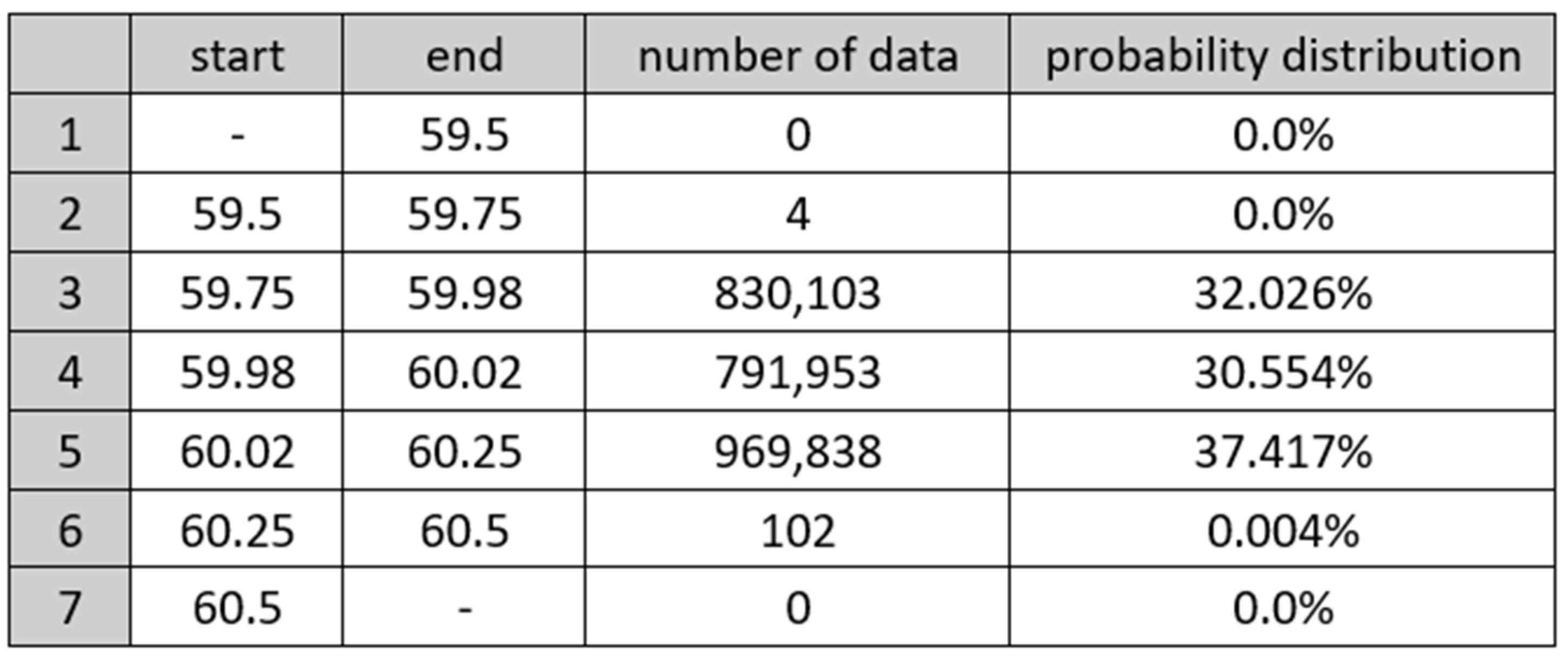
Frequency distribution of May 2020.

Features of SOC Curves
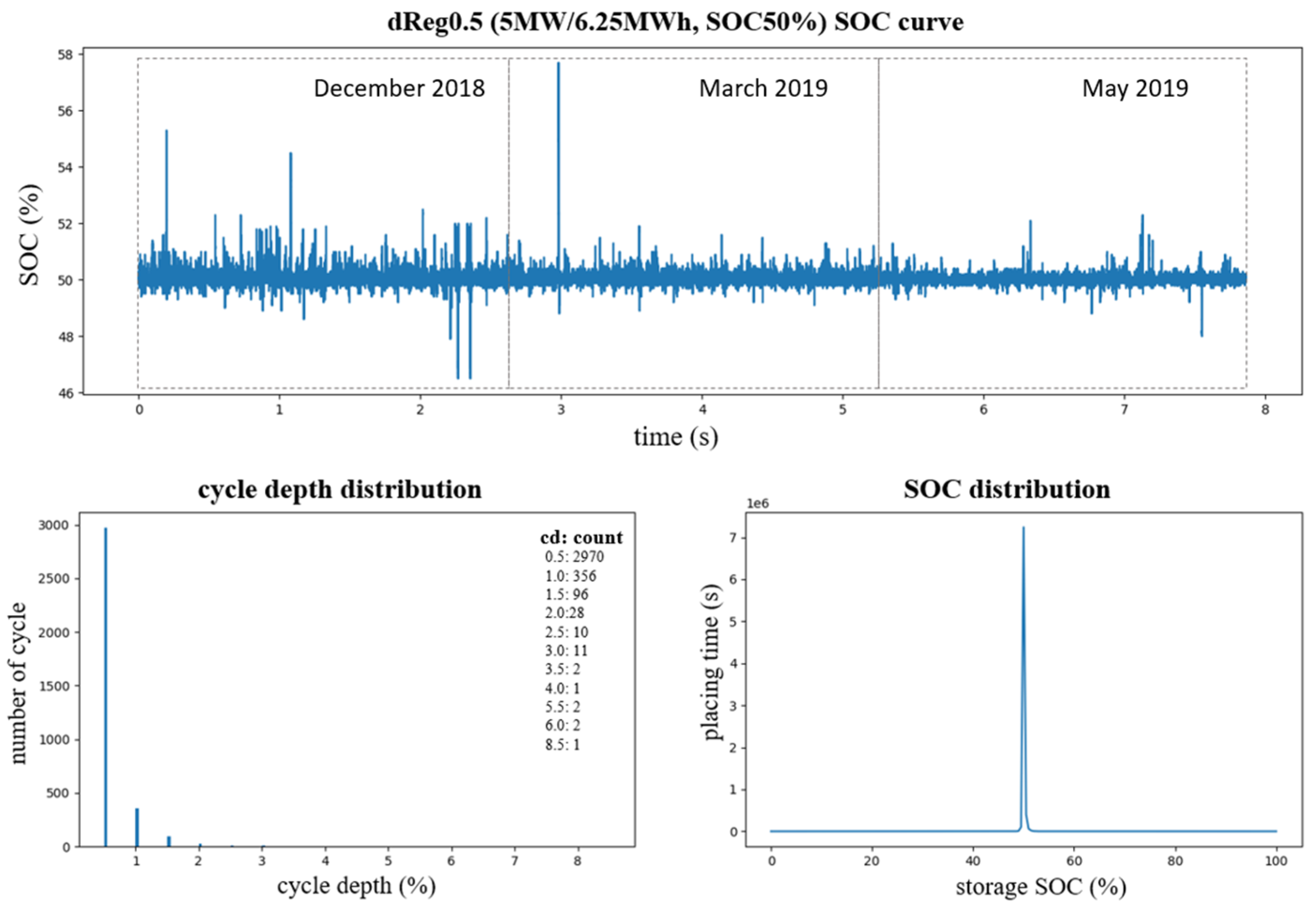
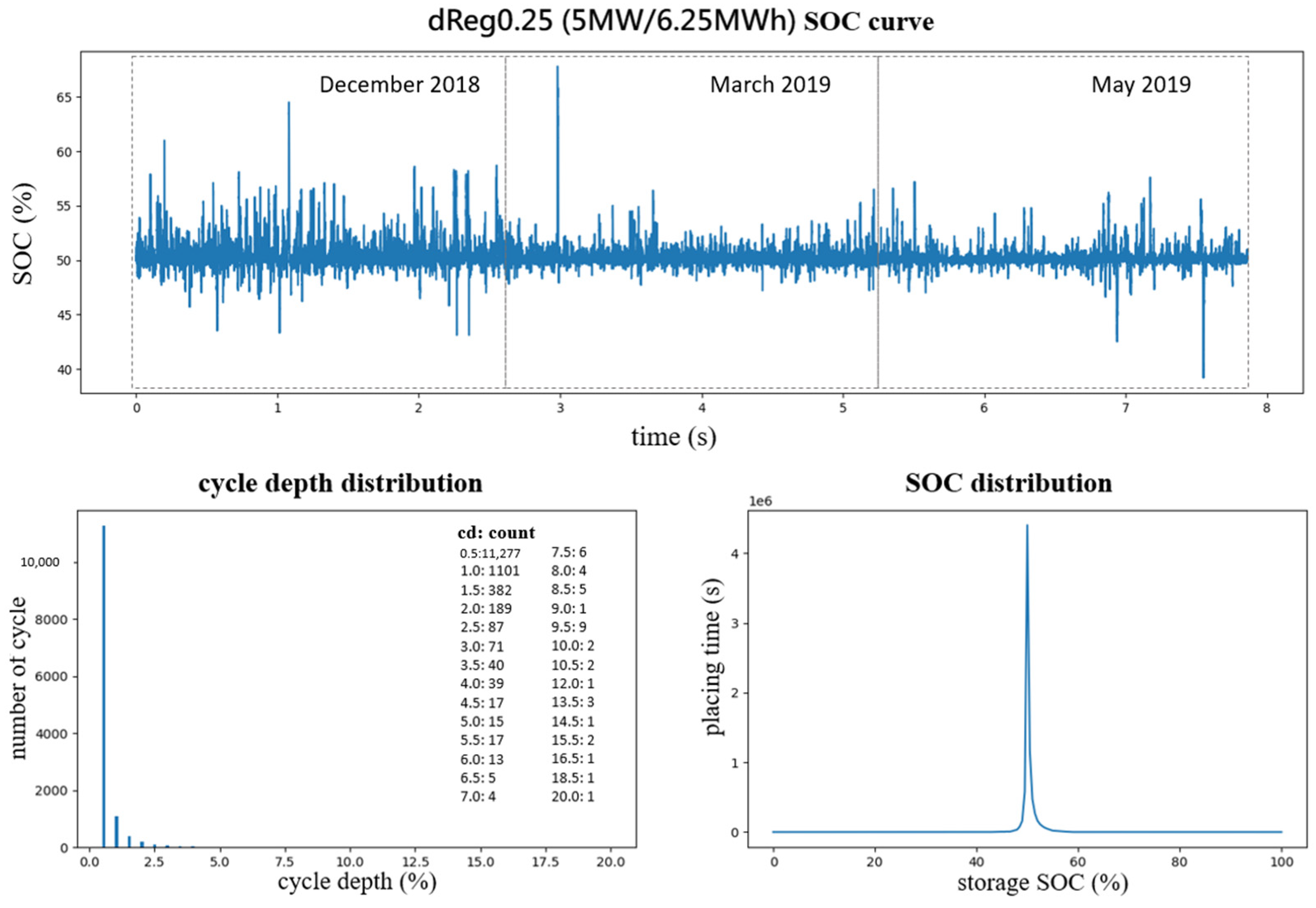
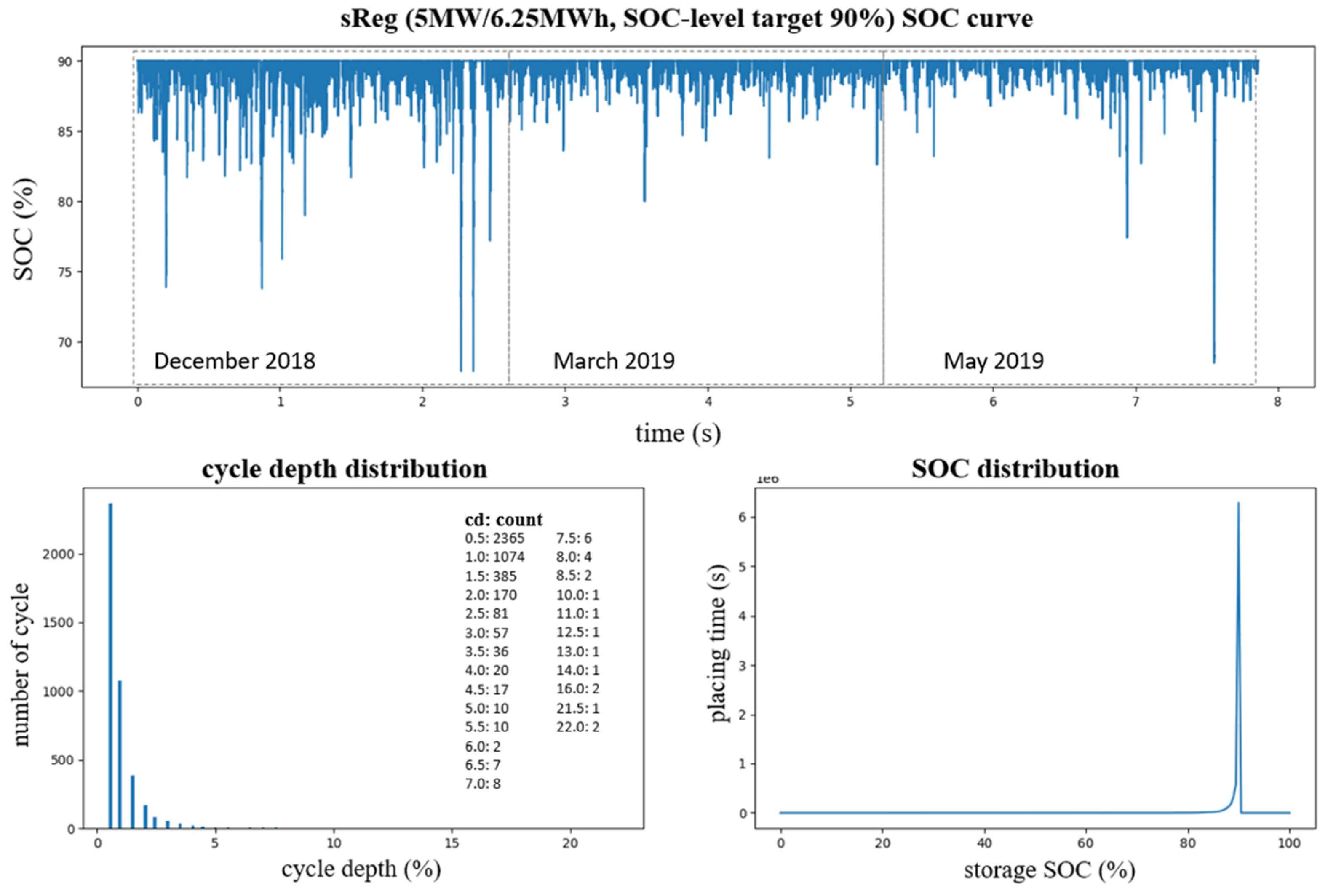
The aging features extracted from SOC curves could be roughly classified into two types, one about cycle depth, and another about storage SOC, which closely relate to cycling aging and calendar aging, respectively. Figure A6, Figure A7 and Figure A8 show the SOC curves for the simulations of Scenarios 2, 5, and 7 based on the three-month frequency, as described in Section 5.2, and the distribution charts of the two main feature types mentioned above.
Figure A6.
SOC curve and aging features of Scenario 2.

Figure A7.
SOC curve and aging features of Scenario 5.

Figure A8.
SOC curve and aging features of Scenario 7.

References
- Smith, K.; Saxon, A.; Keyser, M.; Lundstrom, B.; Cao, Z.; Roc, A. Life prediction model for grid-connected Li-ion battery energy storage system. In Proceedings of the 2017 American Control Conference (ACC), Seattle, WA, USA, 24–26 May 2017. [Google Scholar] [CrossRef]
- Xu, B.; Oudalov, A.; Ulbig, A.; Andersson, G.; Kirschen, D.S. Modeling of Lithium-Ion Battery Degradation for Cell Life Assessment. IEEE Trans. Smart Grid 2016, 9, 1131–1140. [Google Scholar] [CrossRef]
- Padmanabhan, N.; Ahmed, M.; Bhattacharya, K. Battery Energy Storage Systems in Energy and Reserve Markets. IEEE Trans. Power Syst. 2019, 35, 215–226. [Google Scholar] [CrossRef]
- Engels, J.; Claessens, B.; Deconinck, G. Techno-economic analysis and optimal control of battery storage for frequency con-trol services, applied to the German market. Appl. Energy 2019, 242, 1036–1049. [Google Scholar] [CrossRef] [Green Version]
- Beltran, H.; Harrison, S.; Egea-Àlvarez, A.; Xu, L. Techno-Economic Assessment of Energy Storage Technologies for Inertia Response and Frequency Support from Wind Farms. Energies 2020, 13, 3421. [Google Scholar] [CrossRef]
- Diouf, B.; Pode, R. Potential of lithium-ion batteries in renewable energy. Renew. Energy 2015, 76, 375–380. [Google Scholar] [CrossRef]
- Hidalgo-Leon, R.; Siguenza, D.; Sanchez, C.; Leon, J.; Jacome-Ruiz, P.; Wu, J.; Ortiz, D. A survey of battery energy storage system (BESS), applications and environmental impacts in power systems. In Proceedings of the 2017 IEEE Second Ecuador Technical Chapters Meeting (ETCM), Salinas, Ecuador, 16–20 October 2017; pp. 1–6. [Google Scholar] [CrossRef]
- Oudalov, A.; Buehler, T.; Chartouni, D. Utility Scale Applications of Energy Storage. In Proceedings of the 2008 IEEE Energy 2030 Conference, Atlanta, GA, USA, 17–18 November 2008; pp. 1–7. [Google Scholar] [CrossRef]
- Taiwan Electric Power Co., Ltd. Power Dispatching Office, 10 August 2021. Available online: https://etp.taipower.com.tw/web/download/6.%E6%97%A5%E5%89%8D%E8%BC%94%E5%8A%A9%E6%9C%8D%E5%8B%99%E5%B8%82%E5%A0%B4%E4%B9%8B%E4%BA%A4%E6%98%93%E5%95%86%E5%93%81%E9%A0%85%E7%9B%AE%E8%A6%8F%E6%A0%BC.pdf (accessed on 15 May 2022).
- Keil, P.; Schuster, S.F.; Wilhelm, J.; Travi, J.; Hauser, A.; Karl, R.C.; Jossen, A. Calendar Aging of Lithium-Ion Batteries. J. Electrochem. Soc. 2016, 163, A1872–A1880. [Google Scholar] [CrossRef]
- Kassem, M.; Bernard, J.; Revel, R.; Pelissier, S.; Duclaud, F.; Delacourt, C. Calendar aging of a graphite/LiFePO4 cell. J. Power Sources 2012, 208, 296–305. [Google Scholar] [CrossRef] [Green Version]
- Sarre, G.; Blanchard, P.; Broussely, M. Aging of lithium-ion batteries. J. Power Sources 2004, 127, 65–71. [Google Scholar] [CrossRef]
- Stroe, D.; Knap, V.; Swierczynski, M.; Stroe, A.; Teodorescu, R. Operation of a Grid-Connected Lithium-Ion Battery Energy Storage System for Primary Frequency Regulation: A Battery Lifetime Perspective. IEEE Trans. Ind. Appl. 2016, 53, 430–438. [Google Scholar] [CrossRef]
- Kryonidis, G.C.; Nousdilis, A.I.; Pippi, K.D.; Papadopoulos, T.A. Impact of Power Smoothing Techniques on the Long-Term Performance of Battery Energy Storage Systems. In Proceedings of the 2021 56th International Universities Power Engineering Conference (UPEC), Middlesbrough, UK, 31 August 2021–3 September 2021; pp. 1–6. [Google Scholar] [CrossRef]
- Fioriti, D.; Pellegrino, L.; Lutzemberger, G.; Micolano, E.; Poli, D. Optimal sizing of residential battery systems with multi-year dynamics and a novel rainflow-based model of storage degradation: An extensive Italian case study. Electr. Power Syst. Res. 2021, 203, 107675. [Google Scholar] [CrossRef]
- Amzallag, C.; Gerey, J.; Robert, J.; Bahuaud, J. Standardization of the rainflow counting method for fatigue analysis. Int. J. Fatigue 1994, 16, 287–293. [Google Scholar] [CrossRef]
- McInnes, C.; Meehan, P. Equivalence of four-point and three-point rainflow cycle counting algorithms. Int. J. Fatigue 2008, 30, 547–559. [Google Scholar] [CrossRef]
- Stroe, D.-I.; Stan, A.-I.; Diosi, R.; Teodorescu, R.; Andreasen, S.J. Short term energy storage for grid support in wind power applications. In Proceedings of the 2012 13th International Conference on Optimization of Electrical and Electronic Equipment (OPTIM), Brasov, Romania, 24–26 May 2012; pp. 1012–1021. [Google Scholar]
- Mongird, K.; Viswanathan, V.; Alam, J.; Vartanian, C.; Sprenkle, V.; Baxter, R. 2020 Grid Energy Storage Technology Cost and Performance Assessment. Available online: https://www.pnnl.gov/sites/default/files/media/file/Final%20-%20ESGC%20Cost%20Performance%20Report%2012-11-2020.pdf (accessed on 15 May 2022).
Figure 1.
The response curve of the dReg mode.

Figure 2.
The response table of the dReg mode.

Figure 3.
The response table of the sReg mode.

Figure 4.
The response curve of the sReg mode.

Figure 5.
Calendar aging curves.

Figure 6.
Cycling aging curves.

Figure 7.
A schematic diagram for the four-point algorithm.

Figure 8.
A schematic diagram for aging feature extraction.

Figure 9.
A schematic diagram of the applied rainflow counting method of SOC. (a) Raw SOC curve. (b) Curve After filtering continuous values. (c) Only the relative peaks and valleys are left, and the values between the peaks and valleys are removed. (d) Start rainflow cycle counting method.
Figure 9.
A schematic diagram of the applied rainflow counting method of SOC. (a) Raw SOC curve. (b) Curve After filtering continuous values. (c) Only the relative peaks and valleys are left, and the values between the peaks and valleys are removed. (d) Start rainflow cycle counting method.

Figure 10.
A schematic diagram for direct superposition.

Figure 11.
A schematic diagram for superposition.

Figure 12.
A schematic diagram for mapping superposition.

Figure 13.
The result under different SOC levels (dReg0.5).

Figure 14.
The aging ratio of Scenarios 1 to 4.

Figure 15.
The result under different C-rates using dReg0.5 and dReg0.25.

Figure 16.
The aging ratio of Scenarios 5 and 6.

Figure 17.
The result under dReg0.5 and dReg0.25.

Figure 18.
The result under different C-rates (sReg).

Figure 19.
The aging ratio of Scenarios 7 and 8.

Figure 20.
The result under different SOC levels (sReg).

Figure 21.
The aging ratio of Scenarios 7 and 9.

Figure 22.
Net profit under different SOC levels (dReg0.5).

Figure 23.
Net profit under different C-rates using dReg0.5 and dReg0.25.

Figure 24.
Net profit under dReg0.5 and dReg0.25.

Figure 25.
Net profit under different C-rates (sReg).

Figure 26.
Net profit under different SOC levels (sReg).

Figure 27.
Net profit overview under each scenario.


Table 1.
Efficiency level and the price of each mode.
| Efficiency Level | Frequency Regulation Mode | |
|---|---|---|
| 1 | dReg0.25 | 350 |
| 2 | dReg0.5, sReg | 275 |
Table 2.
Specification of simulation scenarios.
| Scenario | Mode | Spec. of BESS | SOC Level Target |
|---|---|---|---|
| 1 | dReg0.5 | 5 MW/6.25 MWh | 70% |
| 2 | dReg0.5 | 5 MW/6.25 MWh | 50% |
| 3 | dReg0.5 | 5 MW/6.25 MWh | 30% |
| 4 | dReg0.5 | 5 MW/3.125 MWh | 50% |
| 5 | dReg0.25 | 5 MW/6.25 MWh | 50% |
| 6 | dReg0.25 | 5 MW/3.125 MWh | 50% |
| 7 | sReg | 5 MW/6.25 MWh | 90% |
| 8 | sReg | 5 MW/12.5 MWh | 90% |
| 9 | sReg | 5 MW/6.25 MWh | 70% |
Table 3.
Overview of comparison between scenarios.
| Battery Life Comparison | Scenarios for Comparison | |
|---|---|---|
| A | dReg0.5 with different SOC level targets | 1,2,3 |
| B | dReg under different C-rates | 2,4(dReg0.5) 5,6(dReg0.25) |
| C | dReg0.5 and dReg0.25under the same spec. | 2,5 |
| D | sReg under different C-rates | 7,8 |
| E | sReg under different SOC level targets | 7,9 |
Table 4.
Battery life overview for each scenario.
| Scenario | Mode | SOC Level | ||
|---|---|---|---|---|
| 1 | dReg0.5 | 5 MW/6.25 MWh | 70% | 189 |
| 2 | dReg0.5 | 5 MW/6.25 MWh | 50% | 210 |
| 3 | dReg0.5 | 5 MW/6.25 MWh | 30% | 228 |
| 4 | dReg0.5 | 5 MW/3.125 MWh | 50% | 195 |
| 5 | dReg0.25 | 5 MW/6.25 MWh | 50% | 189 |
| 6 | dReg0.25 | 5 MW/3.125 MWh | 50% | 165 |
| 7 | sReg | 5 MW/6.25 MWh | 90% | 159 |
| 8 | sReg | 5 MW/12.5 MWh | 90% | 162 |
| 9 | sReg | 5 MW/6.25 MWh | 70% | 180 |
Table 5.
Establishment cost estimation of each scenario.
| Scenario | (MW) | (MWh) | (Thousand NTD) | (Thousand NTD) | (Thousand NTD) | (Thousand NTD) |
|---|---|---|---|---|---|---|
| 1 | 5 | 6.25 | 31,850 | 7350 | 11,900 | 51,100 |
| 2 | 5 | 6.25 | 31,850 | 7350 | 11,900 | 51,100 |
| 3 | 5 | 6.25 | 31,850 | 7350 | 11,900 | 51,100 |
| 4 | 5 | 3.125 | 15,925 | 3675 | 11,900 | 31,500 |
| 5 | 5 | 6.25 | 31,850 | 7350 | 11,900 | 51,100 |
| 6 | 5 | 3.125 | 15,925 | 3675 | 11,900 | 31,500 |
| 7 | 5 | 6.25 | 31,850 | 7350 | 11,900 | 51,100 |
| 8 | 5 | 12.5 | 63,700 | 14,700 | 11,900 | 90,300 |
| 9 | 5 | 6.25 | 31,850 | 7350 | 11,900 | 51,100 |
Publisher’s Note: MDPI stays neutral with regard to jurisdictional claims in published maps and institutional affiliations. |
© 2022 by the authors. Licensee MDPI, Basel, Switzerland. This article is an open access article distributed under the terms and conditions of the Creative Commons Attribution (CC BY) license (https://creativecommons.org/licenses/by/4.0/).
Share and Cite
MDPI and ACS Style
Wu, C.-H.; Jhan, J.-Z.; Ko, C.-H.; Kuo, C.-C. Evaluating and Analyzing the Degradation of a Battery Energy Storage System Based on Frequency Regulation Strategies. Appl. Sci. 2022, 12, 6111. https://doi.org/10.3390/app12126111
AMA Style
Wu C-H, Jhan J-Z, Ko C-H, Kuo C-C. Evaluating and Analyzing the Degradation of a Battery Energy Storage System Based on Frequency Regulation Strategies. Applied Sciences. 2022; 12(12):6111. https://doi.org/10.3390/app12126111
Chicago/Turabian StyleWu, Chen-Han, Jia-Zhang Jhan, Chih-Han Ko, and Cheng-Chien Kuo. 2022. "Evaluating and Analyzing the Degradation of a Battery Energy Storage System Based on Frequency Regulation Strategies" Applied Sciences 12, no. 12: 6111. https://doi.org/10.3390/app12126111
Note that from the first issue of 2016, this journal uses article numbers instead of page numbers. See further details here.