
Selection of Production Reliability Indicators for Project Simulation Model


1
Faculty of Engineering, University of Debrecen, 4028 Debrecen, Hungary
2
Faculty of Economics and Business, University of Debrecen, 4032 Debrecen, Hungary
*
Author to whom correspondence should be addressed.
Appl. Sci. 2022, 12(10), 5012; https://doi.org/10.3390/app12105012
Submission received: 13 April 2022
/
Revised: 3 May 2022
/
Accepted: 6 May 2022
/
Published: 16 May 2022
(This article belongs to the Topic Multi-Criteria Decision Making)
Abstract
:Due to technological enhancements, traditional, qualitative decision-making methods are usually replaced by data-driven decision-making even in smaller companies. Process simulation is one of these solutions, which can help companies avoid costly failures as well as evaluate positive or negative effects. The reason for this paper is twofold: first, authors conducted a Quality Function Deployment analysis to find the most vital reliability indicators in the field of production scheduling. The importance was acquired from the meta-analysis of papers published in major journals. The authors found 3 indicators to be the most important: mean time between failure (MTBF), mean repair time and mean downtime. The second part of the research is for the implementation of these indicators to the stochastic environment: possible means of application are proposed, confirming the finding with a case study in which 100 products must be produced. The database created from the simulation is analyzed in terms of major production KPIs, such as production quantity, total process time and efficiency of the production. The results of the study show that calculating with reliability issues in production during the negotiation of a production deadline supports business excellence.
1. Introduction
Due to the competition among companies, more and more complex products are being manufactured. This also induces the manufacturing of different versions of products, which makes the production process harder to handle and prepare for version changes. Due to mainly the technology development, many aspects of the production can be modeled and evaluated within a short period of time. Such a frequently researched area is the extensive modeling of stochastic processes, e.g., uncertainty in production and risk analysis. However, this goes against the primary aim of modeling: keep the important data in the model, while insignificant ones should be excluded from the model. In this work, reliability indicators are examined in terms of importance—this work provides a meta-analysis in which articles were processed and a conclusion is drawn from the findings. For the analysis, Quality Function Deployment (hereinafter QFD) is used complemented with a multi-criteria decision-making method: the Analytic Hierarchy Process (hereinafter AHP). The combination of these 2 tools supported the authors in the selection of the most important reliability indicators within a list of 15. The most crucial ones are selected and integrated into a simulation model for project scheduling. The database created from the simulation run is analyzed by KPIs in the field of production management.
The paper is organized as follows: the Section 2 is for the brief presentation of the existing literature in reliability management and Quality Function Deployment, Section 3 describes the methodology applied in this paper. Section 4 introduces the research, describes the main results of the meta-analysis as well as providing a brief case study about a production process simulation.
2. Literature Background
2.1. Modeling Project Manufacturing Processes
Due to the challenges of globalization, customers require products that have a high degree of customization. This urges the companies to be flexible in terms of manufacturing, which induces numerous production routings, with multi-purpose tools and machinery and supports the emerge of industry 4.0 [1]. In this special situation, manufacturing companies deal with project manufacturing, because the main features of a product change within a short time, and there is a high chance that the same type of product will never be created anymore [2].
To successfully keep the project management’s “golden triangle”, 4 stages must be performed thoroughly, see [2]:
- Project initiation: The need for special services or products has arisen. The main specification is settled and discussed in financial and other terms, such as agreed time frames.
- Project planning: A more detailed analysis is performed in terms of production: activities, dependencies are revealed, resources are estimated, initial risk assessment is performed.
- Execution: Value creation occurs in this stage: the provision of the services or product manufacturing. In this phase, all the activities are monitored and compared to the plan, and where needs and workflows are carried out.
- Closure: This stage is for the evaluation of positive and negative impacts of the project execution. Drawing conclusions are crucial and these can support later projects.
One of the most critical stages is the project planning, since in this step, the quality, price, delivery time and other indicators are fixed and contracted, and other stages should resonate with these points.
A widely known method for estimating the project lead time is called the Critical Path Method (hereinafter CPM) [3]. This method identifies what activity should be included in the process, what are the dependencies among them, and there should be estimations about the activity times as well. With the use of this method, bottleneck activities (critical activities) can be identified, total project lead time can be calculated, and time slacks can be assigned to those activities that are not considered constraints [4]. The result of this method in the early stage is a project network (G(N,A) network) that represents the production process [5]. Transforming into an operations research model, the following equations are applied [4]:
Objective:
Subject to:
where: are the nodes, z = total project lead time, activity time between and nodes.
Besides this method which contributes valuable information to the decision-makers, literature identifies some drawbacks, as per [4,6]:
- A small change in the activity times can induce a change in the list of bottleneck activities (critical activities).
- It ignores the stochastic feature of the production; the model uses deterministic values for human resources and raw materials.
- It does not provide the possibility of risk management.
- It does not take the resource allocation into account.
As the previously mentioned drawback list displays, CPM conducts production planning in a deterministic way. As a complement of the critical path method, Project Evaluation and Review Technique (hereinafter PERT) is created and used. The main idea behind this methodology is to build a stochastic evaluation of the activity durations with the use of a beta distribution [3,4]:
where: , activity time between and nodes; : minimum time duration of an activity ; : most likely duration of an activity ; : maximum time duration of an activity .
Similarly to CPM method, PERT also has shortcomings [4], especially:
- It only deals with time indicator, it excludes financial calculations.
- PERT uses the result of the CPM method.
- Authors argue that beta is the best distribution for time estimations.
As a conclusion, there is a great need for more sophisticated solutions for modeling production processes loaded with uncertainty and risk. Stochastic CPM provides a great alternative, which combines the merits of the CPM and Monte Carlo Simulation, see [6].
2.2. Reliability Indicators and Risk Analysis
Reliability is a complex concept, and many definitions can be interpreted under it. Is a system reliable when it does not produce a bad quality product? Or is this terminology used for providing information about the condition of a machine? However, it can be stated that both approaches aim at providing quality product for the customers, as well as smooth operation for the production including maintenance and other components of production. According to János Kövesi‘s book [7], there are 4 major categories for the mostly used indicators in production reliability:
- (1)
- Faultlessness: these indicators are created in order to examine the smooth operation of the production system. These are usually time-bounded/calculated ratio: failure rate, mean operation time, probability of failure, probability of faultless operation and mean time between failure.
- (2)
- Reparability: it includes all the indicators which are calculated when a job breaks down and needs to be repaired. These indicators are usually time-bounded or a calculated ratio: mean repair time, mean downtime, recovery intensity, probability of recovery, mean time to repair.
- (3)
- Durability: this category reflects on the durability of the jobs, such as: mean operation time, mean lifespan, q-percent operation.
- (4)
- Storability: this category stands for the storability of the product. This is also an important factor for the customer, as it also has an effect on the perception of quality: mean storage life, percentage of storage time.
Such reliability indicators are in the focus of risk analysis and provide the foundation of the research. In other words, these 15 indicators are analyzed later in the meta-analysis part. As these analyses are concerned, qualitative or subjective calculations are very popular and widely applied in the professional life. Examples for them are the Risk Matrix [8] or the Failure Mode and Effects Analysis (FMEA) [9]. A common drawback is the subjectivity which can mislead the entire analysis, because they do not conform to the need of reproducibility and consistency [10]. That is why quantification and simulation-based methods are emerging [11,12]. However, professionals rely more on data-driven solutions, see papers [13,14]. That is why complex indicators should be created. The previously listed indicators are investigated in the following sections of the authors’ work, which are proven quantitative indicators.
2.3. Quality Function Deployment (QFD)
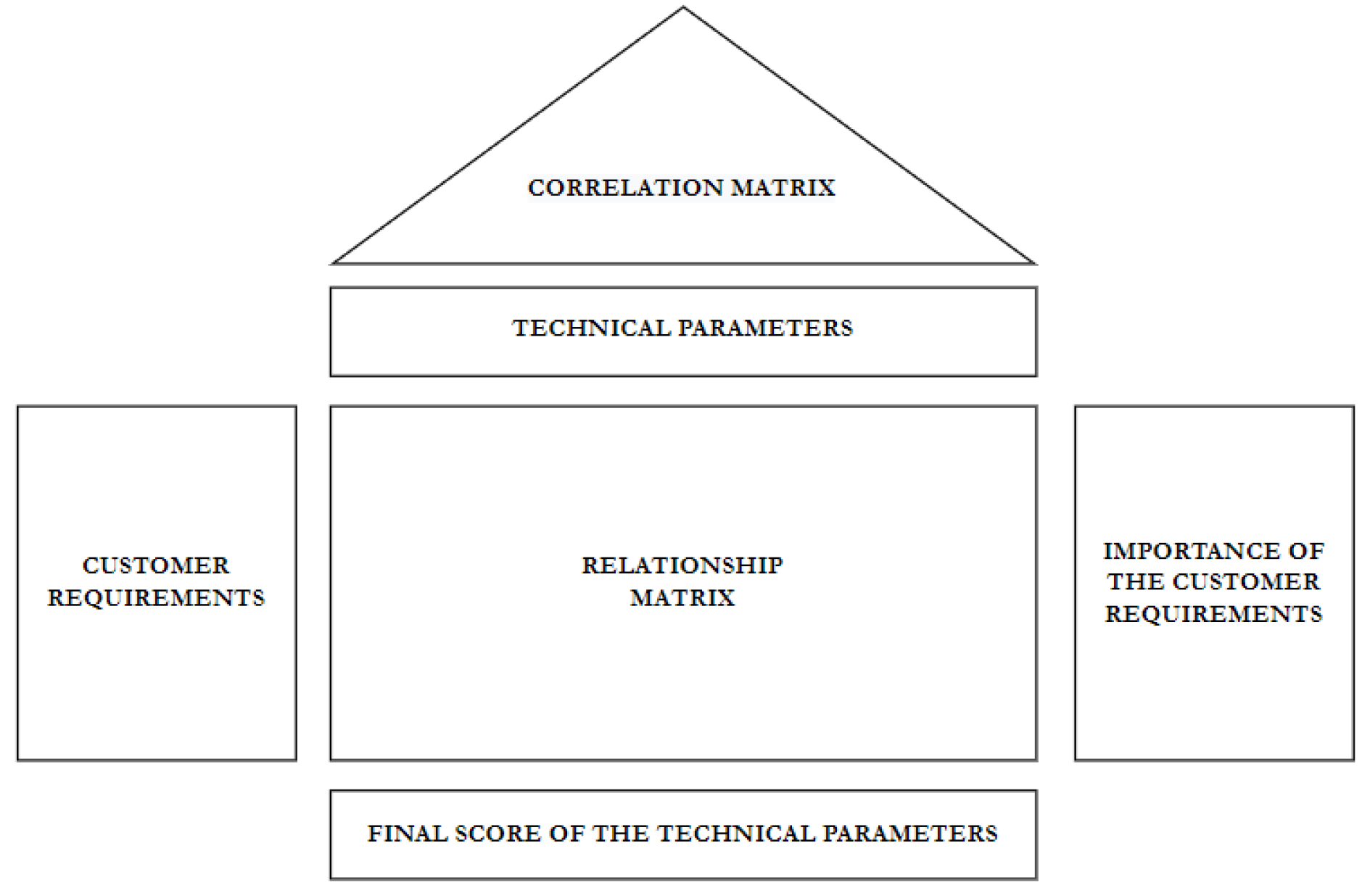
The Quality Function Deployment (or it is known as the House of Quality) is a structured, flexible framework whose focal point is the customer [15]. This methodology was invented in the 1960s for a quick product development by Yoji Akao [9]. The application of this method has spread all over the world. The method became applied in other fields of industry, such as Supply Chain Management [10], Strategic Management [11], education [12], and the list could be expanded.
The aim of this method is to identify the most important customer requirements and technical features of a certain product or service, make priority lists from them, and estimate the correlations, with which positive quality can be maximized. This method is usually complemented with marketing tools (such as survey or interview), however, KANO or VOC models were mostly applied to avoid vagueness in the customer requirements [16,17]. As a consequence, excellent products are being manufactured, which means value for the customer. The method can be described in a house-format, as can be seen in the following figure (Figure 1):
When the importance list from the customer requirements and technical parameters are identified, a relationship matrix should be filled with the following values: “0” means no correlation between a parameter and a requirement, “1” is for slight correlation, “3” stands for a moderate correlation, while “9” represents a strong correlation. Besides this, the direction of the correlation is important [18]. The direction refers to direct or inverse proportional correlation. To determine which technical parameters a company should consider improving, the following equation is applied, which is known as Final Score (FS):
where, is the correlation value of a technical parameter for a requirement , is the weight of the requirement .
To improve the results of the QFD method, quantitative decision-making method can be applied to transform vague requirements into exact ones, such as AHP [18]. An extensive literature review has been published by Medeiros et al. [19] in which the joint application of QFD and AHP methodology is examined with a literature evaluation method. The main conclusion of this paper is that this combination is the most applied one in the following fields: manufacturing, supply chain, higher education, strategy, service, sustainability, marketing, and energy. In another approach of the combination of AHP with different tools, an extensive literature review has been published by Medeiros et al. [19] in which joint application of QFD and AHP methodology is examined with literature evaluation method. A main conclusion of this paper is that this combination is the most applied one in the following fields: manufacturing, supply chain, higher education, strategy, service, sustainability, marketing, and energy. Another approach of the combination of AHP with different tools are investigated as well, and it is stated that QFD is applicable not only for determining the relative weights, but it can also support to calculate the relationship’s intensities among variables [20].
The AHP stands for the Analytic Hierarchy Process, which is a multi-criteria decision-making tool invented by Saaty [21]. One of the main advantages comes from the pairwise comparison, which makes differently scaled requirements comparable with one another. As far as the execution of such a method is concerned, it is entered in a matrix, its columns and rows represent the same elements: Therefore, the main diagonal of the matrix remains 1, but the matrix is mostly filled in with the following values, see [22]:
1: Equal importance
3: Moderate importance
5: Strong importance
7: Very strong importance
9: Extreme importance
2,4,6,8: Intermediate values, when compromise is needed.
Reciprocals: when element is compared to element , the reciprocal should be assigned when element is compared to element in order to keep the consistency of the calculation [21,23]. As further steps of the method, standardization of weights as well as consistency index (CI) calculation takes place to ensure an objective decision result.
The method is easily adoptable in management decision-making, similar to the combination of a decision tree and AHP in construction project [24], or the mix of AHP and DEA (Data envelopment Analysis) used in transportation problem solving [25], but it is used in failure analysis complemented with FMEA [26]. As it was stated above in this section, QFD method is a widely known tool to integrate with AHP.
There are debates among professionals to determine which multi-criteria decision-making tool is the best for a certain decision situation: In the research by Sarraf and McGuire [27], AHP performs exceptionally in a design of safe transportation route together with the PROMETHEE, while another known method, such as TOPSIS, performed poorly in this research. In another research [28], a comparison of AHP and MADA has taken place. As far as the final decision is concerned, AHP and MADA had very similar results.
3. Materials and Methods
3.1. Research Goal, Hypotheses
The primary aim of the authors is to apply the Quality Function Deployment (QFD) method for selecting requirements and indicators for professionals in the field of production process simulation. Furthermore, the implementation of selected indicators into a simulation model is proposed:
Goal 1: To find out what are the most important reliability indicators based on the result of a meta-analysis and Quality Function Deployment.
Goal 2: Fit the selected reliability indicators to a project simulation model.
Goal 3: Analyze the dataset gathered from the proposed simulation model.
Besides the goals of the research, some research questions have arisen, which will be investigated in the results part:
RQ1: What are the most important reliability indicators for project scheduling?
RQ2: How can they be implemented in a decision-making process?
As a preliminary assumption, authors believed that the mean time between failure and mean time to repair are the most important indicators to implement to a simulation model and therefore proposed hypotheses considering the possible implementation opportunities for the simulation model.
Hypothesis 1.
Quality Function Deployment supports the ranking and the selection of reliability indicators.
Hypothesis 2.
MTBF and MTTR reliability indicators are the most important factors of production.
Hypothesis 3.
MTBF can be implemented in stochastic process simulation in a way where every n-th simulation iteration induces failure.
Hypothesis 4.
Total project time can be estimated with the use of modified stochastic CPM model.
3.2. Operationalization, Steps of the Process
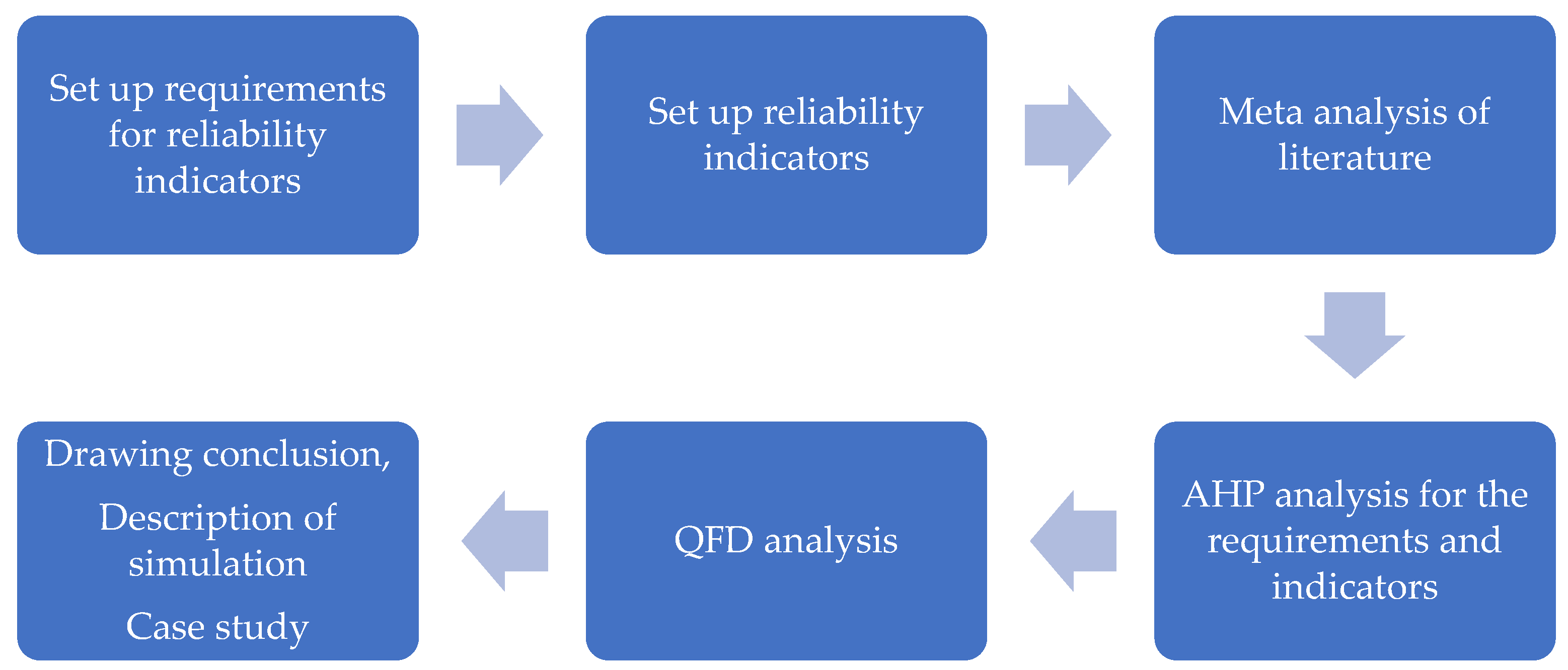
The next figure (Figure 2) represents the process that the authors follow for both the meta-analysis and experiment phases:
As a first step of the research, requirements and indicators were collected and evaluated from the literature [29,30,31,32,33,34,35,36,37,38,39,40,41,42,43]. This input supported the authors to make AHP analyses with the use of which the importance of these components were calculated and consistency calculations carried out. Additionally, correlations among the requirements and indicators were assessed with the use of 1-3-9 values by the conventional QFD relationship matrix [13]. As an outcome, the most crucial components are selected which can be implemented in a production process simulation method. As a closure, a pseudocode for making such a simulation is described, as well as a case study created in order to present how the findings work in practical environment.
4. Results
4.1. Meta-Analysis
To develop a mathematical model, a well thought-out literature evaluation should be created. The authors reviewed engineering- and business-related journals that are indexed in academically acknowledged databases. To reveal the most suitable results, the following databases were visited and articles were collected from the following: ScienceDirect, Scopus, Elsevier.
An additional filter to our search was the date of publication: for the most appropriate findings, only recent (since 2017) articles were processed.
The authors selected 8 keywords for the search and created a database for the findings. After a careful and thorough review, the relevant articles remained in the database.
The keyword structure was followed:
(process OR system OR machine OR production OR manufacturing)
AND
(reliability OR uncertainty OR stochastic)
AND
(simulation OR analysis)
AND
(reliability OR uncertainty OR stochastic)
AND
(simulation OR analysis)
Out of the 15 indicators listed in the literature review section, the authors selected 7, which can be directly connected to machine failure and its repair. The scope of the project is the application of indicators that uses time: mean operation time, probability of faultless operation, mean time between failure, mean repair time, mean downtime, mean time to repair, mean lifespan.
Out of the 15 indicators listed in the literature review section, the authors selected 7 which can be directly connected to machine failure and its repair given in time measurement unit: mean operation time, probability of faultless operation, mean time between failure, mean repair time, mean downtime, mean time to repair, mean lifespan.
Thus, the following indicators were excluded from the scope of the research: failure rate, probability of failure, recovery intensity, probability of recovery, q-percent operation, mean storage life, percentage of storage time. The reason for this decision is simple: the previously listed indicators either provide the likelihood of a problem or it is connected to the product rather than the production process (e.g., percentage of storage time).
The following table (Table 1) present the authors’ finding: Is a certain indicator really crucial for the process analysis to mention it or work with? In this process, relevant articles were processed, with the focus on manufacturing-related production examples or theoretical studies. In the matrix below, “M” represents mentions, which means the application of the indicator in a case study, or—in case of theoretical study—introduces the indicator. “-” symbol indicates the absence of the indicator from that particular article.
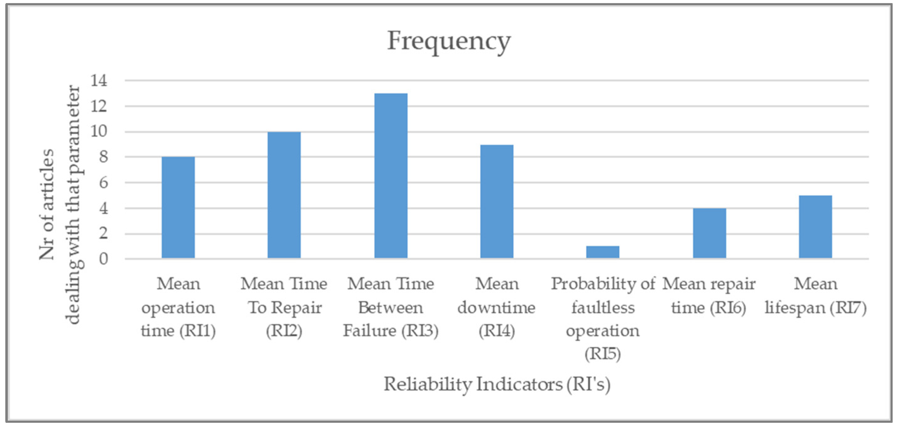
The examined papers show that the most used indicators are mean time between failure (MTBF), mean time to repair (MTTR), mean downtime, and mean operation time. This is mainly because of the ease of use, calculation, and implementation of these values. The least ones were considered harder in calculating probabilities or indicators that can be calculated from other parameters of reliability. Alternatively, the lifespan of the machinery is just considered to be long-term. The count of mentions can be seen in the figure (Figure 3) below:
4.2. Results of the Quality Function Deployment
For the determination of the customer requirements, a brainstorming activity, as well as a focus group interview took place with professionals in the field of quality and production. At the end of the activity, the following requirements were established and defined:
- Time-based (CR1): A crucial part of production scheduling is the time. The time consequences of probable problems should be implemented in the model.
- Measurable (CR2): All the included indicators should be described quantitatively.
- Correlation among failures (CR3): When a model is created, the dependency among problems should be described to examine domino-effect.
- Frequency (CR4): A frequency of a certain problem can be given or calculated.
- Critical Path change (CR5): In the case of time increase, total process time and critical path should be evaluated.
- Integration to production scheduling method (CR6): A certain component, indicator or parameter only helps the decision-maker when it is logically built in the model.
- The speed of calculation (CR7): The execution of a stochastic model should take as little time as it is possible. The calculation speed depends on the complexity of the indicator built in the simulation.
During the brainstorming event, a rank and priority was set to each alternative, which was used for an AHP method. The reason for choosing this method is the wide acceptance in numerous disciplines; moreover, it should not be fully consistent to obtain acceptable results, and more importantly, its ability to handle qualitative and quantitative attributes as well as requiring full focus due to dealing with the same questions from two different points of view (compare to , then compare to ) [44,45].
There was consensus among the participants that the “Time-based” and “Integration to production scheduling method” are equally favored, but are dominant requirements. The result of the pairwise comparison is considered to be consistent because the Consistency Index falls between the acceptance range (CI = 0.104). The standardized importance table can be seen in the following table (Table 2):
The most important criteria in this respect are the CR1 (Time-based) and CR6 (Integration to scheduling method), while the least important criteria are CR3 (Correlation among failures), CR7 (Calculation speed), and CR4 (Frequency).
The result was built in the QFD method, where criteria are prioritized based on their importance; 0-1-3-9 values were assigned to the relationship matrix where the correlation among customer requirements and technical parameters is identified. In this process, special attention went to understand the objective of the criteria (is the smaller or the higher value more beneficial for the customer?); 0 values were only added when there was no connection between the criteria and the indicator. Such an example is the rate or probability calculations regarding the criteria titled “Time-based”. These indicators only show a ratio, and it is hard, or impossible to translate them into time value. As an opposite, all indicators performed well in the criteria called Integration to production scheduling method. Most of the literature collected during the research dealt with the implementation of production scheduling method, or stated that each indicator can be integrated into production arrangement. The following table (Table 3) presents the relationship matrix and the importance values by the QFD.
The most important reliability indicators are the mean time between failure and mean downtime values. When a more detailed analysis is carried out on the alternatives, it can be stated that the mean operation time and mean downtime correlate with each other. Additionally, mean repair time is included in the mean downtime indicator, because repair only takes place when there is no operation on the machinery. The least weight is assigned to speed of calculation, because in such a scenario analysis of a project, there can be enough time to apply stochastic process modeling.
4.3. Implementation of the Selected Indicators to a Process Simulation Model
As it can be inferred from the result of the QFD method, there are two outstanding indicators, which are advised to be built in the process simulation. These indicators can be treated at the same time in the process simulation model.
The MTBF indicator can be interpreted in two different ways:
- Based on experimental data or professional estimation, an exact value can be assigned to trigger the failure in the activity. This is done by accumulating total process times and examining the value by mod operator.
- The other approach is providing information about the failure in cycle format. This can be very useful when a production process is described in network format (e.g., CPM) and stochastic methodology is applied. The stochastic CPM can also be applied when a high volume production is modeled and the activities should wait for the end of the process. A decision-maker can have an estimate about how frequently a certain failure repeats itself, e.g., every 5th run is affected by that particular problem.
The aforementioned are considered easier ways to implement this idea in coding. This variation is described in the following table in the Pseudocode (Algorithm 1):
| Algorithm 1 ReliabilitySimulation. | |
| 1: | seti to 1, |
| 2: | setsetShift to 2, // 2 shifts per day |
| 3: | setsetMinutes to 480, // 8 h in a shift |
| 4: | settotalProcessTime to 0, |
| 5: | setcumulatedTPT to 0, |
| 6: | setnrDays to 0, |
| 7: | setnrShifts to 0, |
| 8: | setactivityDuration, //array |
| 9: | setproblemList //problemCount, activityAffected, MTBFCycle, meanDownTime |
| 10: | fori to n |
| 11: | randomizeactivityDuration |
| 12: | for each problem n |
| 13: | if i % problemList[MTBFCycle] == 0 then |
| 14: | activityDuration[n] = activityDuration[n] + problemList[meanDownTime] |
| 15: | end if |
| 16: | else activityDuration[n] = activityDuration[n] |
| 17: | end for |
| 18: | solvetotalProcessTime → min! |
| 19: | createsensitivityReport |
| 20: | cumulatedTPT = cumulatedTPT + totalProcessTime, |
| 21: | nrDays = cumulatedTPT / (setShift ∗ setMinutes) |
| 22: | nrShifts = cumulatedTPT / setMinutes |
| 23: | copyi, activityDuration, totalProcessTime, cumulatedTPT, sensitivityReport, nrDays, |
| nrShifts | |
| 24: | end for |
The result of the modified process simulation shows how many times a certain problem occurred and how much time the machine spends out of production (downtime). In this case, downtime is not further categorized, but it can also be done by breaking down the process into smaller activities. Additionally, cost calculations can be fit to the model, but this was out of scope in this research.
4.4. Experiment
This study is about a production process which is carried out in a job shop technology. The manufacturing process confirms the use of Critical Path Method; 100 products should be manufactured, and the company wants an estimation about the total lead time of the project. As it was stated previously, all the activity should be accomplished to start the next production process. For this purpose, a CPM is the best-fit model. The network of the processes can be seen in Figure 4.
The production process is fictional, the authors wanted to present a moderately difficult process with parallel and sequential (dependent) activities. The nodes represent the events which resulted in activities. This naming convention helps professionals consctuct the equations for the graph. The activity times and their distributions for the simulation can be seen in the next table (Table 4). Beta-distributions were used for each activity, because it is used in PERT analysis as well [4], furthermore its shape is symmetric when and parameters are equal. The main information about the process can be examined in the next table (Table 4):
The reliability problems are given in a table format (see Table 5), which includes all the necessary information regarding the process simulation, such as which activity is affected by the problem, what is the cycle number for MTBF indicator (=this represents that reliability issue takes place at every nth cycle), as well as the time in which the machine is not available (=repair + waiting for repair). A domino-effect can also be modeled by placing the same MTBF value for more problems, or common multiples can also be used for the modeling correlation among reliability issues.
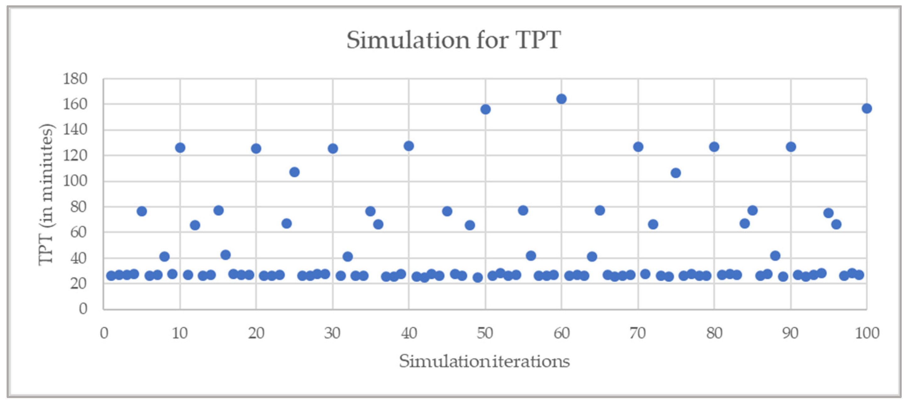
When all the inputs were available, a 100-iteration-simulation was loaded on the basis of the Pseudocode presented in the previous chapter. The number of iterations in the simulation was in accordance with the number of products to be manufactured. The simulation was programmed in Visual Basic Application (VBA), and the result was collected in a spreadsheet database. The reason for using this framework is the flexibility and scalability that provides a great tool for managers in decision-making [46]. The next figure (Figure 5) presents the total process times of each simulated project iterations. Most of the simulated values are around the deterministic (median) value, but there are some outlier iterations. These extreme values are due to the downtime of the production which is caused by a reliability issue. At some point of iteration, more issues occurred, so downtimes are accumulated and added to the total process time. The accumulated project run time is 4688 min including reliability issues in the production.
Applying a linear regression on the accumulated total process time values, the following equation can be used for describing and forecasting (:
This means that the average total process time to manufacture a product is significantly more than it is described deterministically.
As a great contribution, critical paths of these process runs were investigated. During the analysis, three critical paths were distinguished; let us call them A, B, C that can be seen in Table 6.
One of the mostly found critical paths was the “A” path with 73 out of 100 runs. The other paths are less significant, but it is advisable to pay attention to the identified critical paths because they do not have slack time. These activities should be analyzed more in detail, and problems and reliability issues should be mapped. Furthermore, workarounds should be invented in order to reduce downtime or the occurrence of the problem to increase capacity.
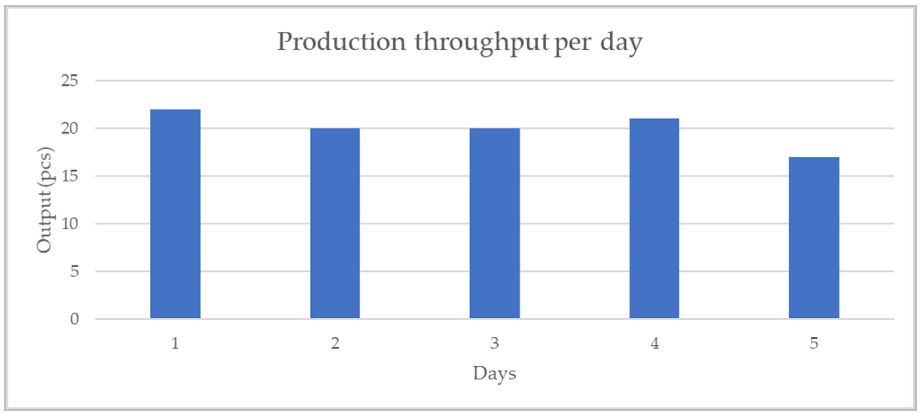
As a last step of the analysis, production throughput was analyzed. Accumulated total process times were used for breaking down the activities into shifts and days. This supported in making an analysis about the progression of the full project execution, see Figure 6.
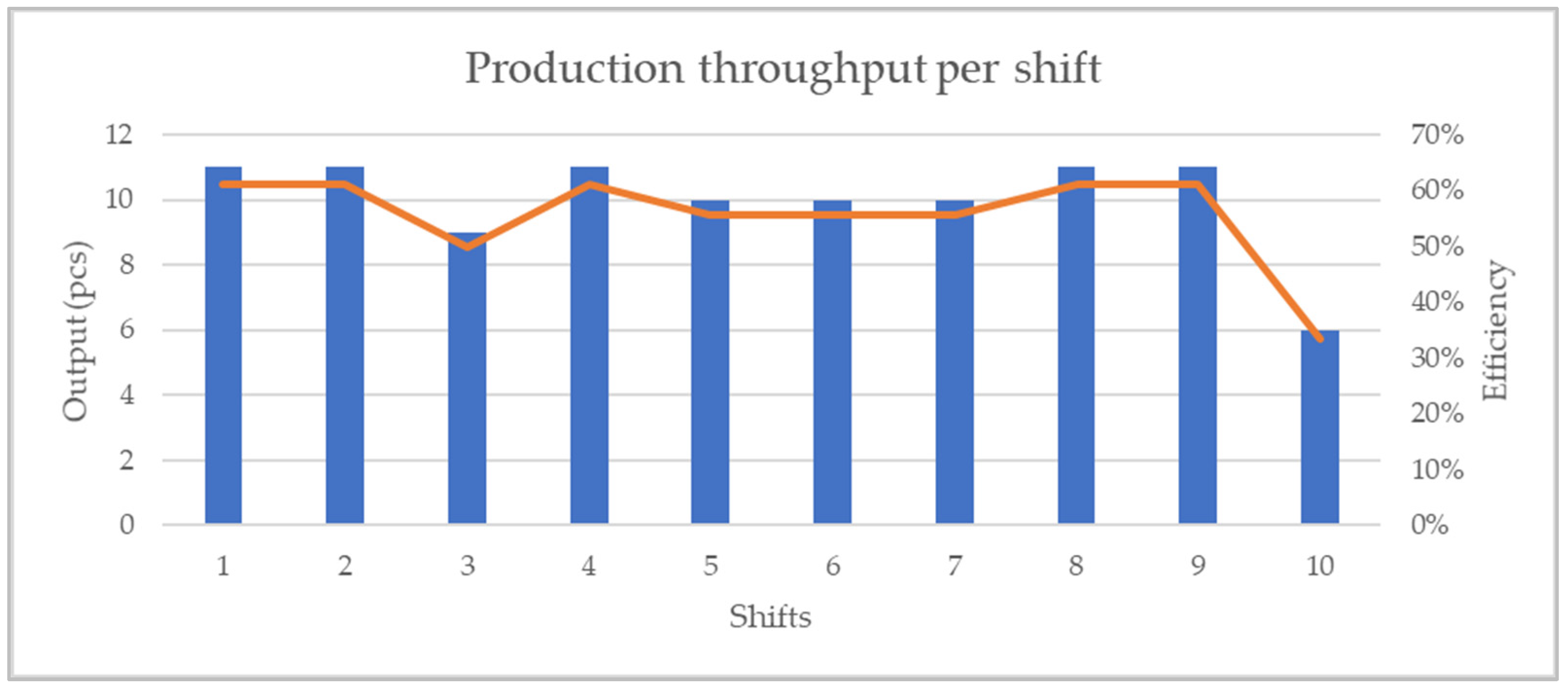
Based on the daily production output, it can be stated that more or less the same quantity could be done within a day. The total project time for 100 products was 4688 min. Supposing that this production structure works in 2 shifts/day and 480 min/shift schedule, the production time takes approximately 10 whole shifts (or 5 days). Not all the day/shifts were used to complete the order of 100 products; see the last day/shift, where approximately 2 h remains unscheduled. This is represented by an efficiency indicator that can be seen in the following figure (Figure 7).
Efficiency is indicated by an orange line seen in the above figure (Figure 7) and presents the efficiency value compared to a deterministic CPM value. Deterministic CPM was calculated and the capacity of the shift was computed:
As a next step, the result of the simulation was compared to this theoretical capacity value, and efficiency was determined in the secondary axis. The efficiency was around 60%, and the other 40% is due to the reliability issues built in the simulation model.
5. Conclusions
In this study, a Quality Function Deployment methodology was applied to identify the most important reliability indicators in production. The priority was set based on recent papers published in quality journals. As a contribution of this paper, the combination of QFD and AHP methodologies proved that in production scheduling, the MTBF, MTTR, mean downtime, and mean operation time are the most important indicators. Based on the results of the research, a pseudocode for the Monte Carlo simulation was created and complemented with the most important reliability indicators. The simulation proposal was created in Visual Basic Application, and the result of the case study was analyzed. With the analysis of the database created from the case study, decision-makers could see the key performance indicators, such as efficiency of the production, and possible total project time including reliability risks. Considering the results of the study, it turned out that approximately 10 shifts or 5 days would be ideal for the production, and this time interval is advised for decision-makers to plan the contract or delivery deadline of the final product.
As a further possible research direction, cost calculation can be applied, and a decision-making framework can be formulated including risk preference of the decision-maker together with the consideration of external risks, such as uncertainty in the supply. This can be also integrated in game theory, or it can be used for creating an effective negotiation strategy. The presented method is scalable and flexible enough to implement in any fields of production.
Author Contributions
Conceptualization, L.P.P. and L.N.; Methodology, L.P.P. and L.N.; Supervision, I.B.; Validation, L.P.P. All authors have read and agreed to the published version of the manuscript.
Funding
This research received no external funding.
Institutional Review Board Statement
Not applicable.
Informed Consent Statement
Not applicable.
Data Availability Statement
Not applicable.
Conflicts of Interest
The authors declare no conflict of interest.
References
- Espinoza Pérez, A.T.; Rossit, D.A.; Tohmé, F.; Vásquez, Ó.C. Mass customized/personalized manufacturing in industry 4.0 and blockchain: Research challenges, main problems, and the design of an information architecture. Inf. Fusion 2022, 79, 44–57. [Google Scholar] [CrossRef]
- Project Management Institute. A Guide to the Project Management Body of Knowledge: (PMBOK® Guide), 6th ed.; Project Management Institute: Newtown Square, PA, USA, 2017. [Google Scholar]
- Ragsdale, C.T. Spreadsheet Modeling & Decision Analysis: A Practical Introduction to Business Analytics; Cengage Learning: Stamford, CT, USA, 2021. [Google Scholar]
- Wayne, W.L. Operations Research: Applications and Algorithms; Duxbury Press: Belmont, CA, USA, 2004. [Google Scholar]
- Temesi, J.; Varró, Z. Operációkutatás; Akadémiai Kiadó: Budapest, Hungary, 2014. [Google Scholar]
- Pusztai, L.; Kocsi, B.; Budai, I. Making engineering projects more thoughtful with the use of fuzzy value-based project planning. Pollack Period. 2019, 14, 25–34. [Google Scholar] [CrossRef]
- Kövesi, J.; Erdei, J. Minőség És Megbízhatóság a Menedzsmentben; Typotex: Budapest, Hungary, 2011. [Google Scholar]
- Ferreira, S.; Silva, F.J.G.; Casais, R.B.; Pereira, M.T.; Ferreira, L.P. KPI development and obsolescence management in industrial maintenance. Procedia Manuf. 2019, 38, 1427–1435. [Google Scholar] [CrossRef]
- Korayem, M.H.; Iravani, A. Improvement of 3P and 6R mechanical robots reliability and quality applying FMEA and QFD approaches. Robot. Comput.-Integr. Manuf. 2008, 24, 472–487. [Google Scholar] [CrossRef]
- Abusalem, O.; Bertalan, N.; Kocsi, B. Implementing quantitative techniques to improve decision making in construction projects: A case study. Pollack Period. 2019, 14, 223–234. [Google Scholar] [CrossRef]
- Kocsi, B.; Matonya, M.M.; Pusztai, L.P.; Budai, I. Real-time decision-support system for high-mix low-volume production scheduling in industry 4.0. Processes 2020, 8, 912. [Google Scholar] [CrossRef]
- Lux, A.; Mawo De Bikond, J.; Etienne, A.; Quillerou-Grivot, E. FMEA and consideration of real work situations for safer design of production systems. Int. J. Occup. Saf. Ergon. 2016, 22, 557–564. [Google Scholar] [CrossRef]
- Adedigba, S.A.; Oloruntobi, O.; Khan, F.; Butt, S. Data-driven dynamic risk analysis of offshore drilling operations. J. Pet. Sci. Eng. 2018, 165, 444–452. [Google Scholar] [CrossRef]
- Mazumder, R.K.; Salman, A.M.; Li, Y. Failure risk analysis of pipelines using data-driven machine learning algorithms. Struct. Saf. 2021, 89, 102047. [Google Scholar] [CrossRef]
- Karasan, A.; Ilbahar, E.; Cebi, S.; Kahraman, C. Customer-oriented product design using an integrated neutrosophic AHP & DEMATEL & QFD methodology. Appl. Soft Comput. 2022, 118, 108445. [Google Scholar] [CrossRef]
- Rampal, A.; Mehra, A.; Singh, R.; Yadav, A.; Nath, K.; Chauhan, A.S. Kano and QFD analyses for autonomous electric car: Design for enhancing customer contentment. Mater. Today Proc. 2022. [Google Scholar] [CrossRef]
- Hashim, A.M.; Dawal, S.Z.M. Kano model and QFD integration approach for ergonomic design improvement. Procedia-Soc. Behav. Sci. 2012, 57, 22–32. [Google Scholar] [CrossRef] [Green Version]
- Chan, L.-K.; Wu, M.-L. Quality function deployment: A literature review. Eur. J. Oper. Res. 2002, 143, 463–497. [Google Scholar] [CrossRef]
- de Oliveira, L.M.V.; Santos, H.F.D.; de Almeida, M.R.; Costa, J.A.F. Quality function deployment and analytic hierarchy process: A literature review of their joint application. Concurr. Eng. 2020, 28, 239–251. [Google Scholar] [CrossRef]
- Ho, W. Integrated analytic hierarchy process and its applications—A literature review. Eur. J. Oper. Res. 2008, 186, 211–228. [Google Scholar] [CrossRef]
- Saaty, T.L. The analytic hierarchy process: Decision making in complex environments. In Quantitative Assessment in Arms Control; Springer: Berlin/Heidelberg, Germany, 1984; pp. 285–308. [Google Scholar] [CrossRef]
- Saaty, T.L. How to make a decision: The analytic hierarchy process. Eur. J. Oper. Res. 1990, 48, 9–26. [Google Scholar] [CrossRef]
- Saaty, R.W. The analytic hierarchy process—What it is and how it is used. Math. Model. 1987, 9, 161–176. [Google Scholar] [CrossRef] [Green Version]
- Maceika, A.; Bugajev, A.; Šostak, O.R.; Vilutienė, T. Decision tree and AHP methods application for projects assessment: A case study. Sustainability 2021, 13, 5502. [Google Scholar] [CrossRef]
- Gupta, P.; Mehlawat, M.K.; Aggarwal, U.; Charles, V. An integrated AHP-DEA multi-objective optimization model for sustainable transportation in mining industry. Resour. Policy 2018, 74, 101180. [Google Scholar] [CrossRef]
- Li, H.; Díaz, H.; Guedes Soares, C. A failure analysis of floating offshore wind turbines using AHP-FMEA methodology. Ocean. Eng. 2021, 234, 109261. [Google Scholar] [CrossRef]
- Sarraf, R.; McGuire, M.P. Integration and comparison of multi-criteria decision making methods in safe route planner. Expert Syst. Appl. 2020, 154, 113399. [Google Scholar] [CrossRef]
- Díaz, H.; Loughney, S.; Wang, J.; Guedes Soares, C. Comparison of multicriteria analysis techniques for decision making on floating offshore wind farms site selection. Ocean Eng. 2022, 248, 110751. [Google Scholar] [CrossRef]
- Huerta, J.R.; Silva, R.S.; De Tomi, G.; Ayres da Silva, A.L.M. A dynamic simulation approach to support operational decision-making in underground mining. Simul. Model. Pract. Theory 2022, 115, 102458. [Google Scholar] [CrossRef]
- Friederich, J.; Lazarova-Molnar, S. Towards data-driven reliability modeling for cyber-physical production systems. Procedia Comput. Sci. 2021, 184, 589–596. [Google Scholar] [CrossRef]
- Chen, X.; An, Y.; Zhang, Z.; Li, Y. An approximate nondominated sorting genetic algorithm to integrate optimization of production scheduling and accurate maintenance based on reliability intervals. J. Manuf. Syst. 2020, 54, 227–241. [Google Scholar] [CrossRef]
- O’Brien, E.M.; Baily, S.A.; Birnbaum, E.R.; Chapman, C.; Espinoza, E.A.; Faucett, J.A.; Hill, J.O.; John, K.D.; Marroquin, P.S.; McCrady, R.C.; et al. Novel design and diagnostics improvements for increased production capacity and improved reliability at the los alamos isotope production facility. Nucl. Instrum. Methods Phys. Res. Sect. A Accel. Spectromet. Detect. Assoc. Equip. 2020, 956, 163316. [Google Scholar] [CrossRef]
- Marchi, B.; Zanoni, S.; Jaber, M.Y. Economic production quantity model with learning in production, quality, reliability and energy efficiency. Comput. Ind. Eng. 2019, 129, 502–511. [Google Scholar] [CrossRef]
- Görkemli, L.; Kapan Ulusoy, S. Fuzzy bayesian reliability and availability analysis of production systems. Comput. Ind. Eng. 2010, 59, 690–696. [Google Scholar] [CrossRef]
- Kumar, N.S.H.; Manjunath, C.; John, R.P.; Chand, R.P.; Madhusudhana, S.; Venkatesha, B.K. Reliability, availability and maintainability study of 6.5 cubic meters shovel and 60 tone dumper in a surface limestone mine. Mater. Today Proc. 2022, 54, 199–204. [Google Scholar] [CrossRef]
- Li, Y.; Coolen, F.P.A.; Zhu, C. A practical reliability design method considering the compound weight and load-sharing. Int. J. Approx. Reason. 2020, 127, 17–32. [Google Scholar] [CrossRef]
- Harmon, V.L.; Wolfrum, E.; Knoshaug, E.P.; Davis, R.; Laurens, L.M.L.; Pienkos, P.T.; McGowen, J. Reliability metrics and their management implications for open pond algae cultivation. Algal Res. 2021, 55, 102249. [Google Scholar] [CrossRef]
- He, Y.; Zhang, H.; Wang, P.; Huang, Y.; Chen, Z.; Zhang, Y. Engineering application research on reliability prediction of the combined DC-DC power supply. Microelectron. Reliab. 2021, 118, 114059. [Google Scholar] [CrossRef]
- Alavian, P.; Eun, Y.; Liu, K.; Meerkov, S.M.; Zhang, L. The (α, β)-precise estimates of MTBF and MTTR: Definition, calculation, and observation time. IEEE Trans. Autom. Sci. Eng. 2020, 18, 1469–1477. [Google Scholar] [CrossRef]
- Leite, M.; Costa, M.A.; Alves, T.; Infante, V.; Andrade, A.R. Reliability and availability assessment of railway locomotive bogies under correlated failures. Eng. Fail. Anal. 2022, 135, 106104. [Google Scholar] [CrossRef]
- Dubový, D.; Famfulík, J.; Richtář, M. Determination of operational reliability of firefighting special vehicles. Transp. Res. Procedia 2021, 55, 126–132. [Google Scholar] [CrossRef]
- Kavyashree, N.; Supriya, M.C.; Lokesh, M.R. Site reliability engineering for IOS mobile application in small-medium scale industries. Glob. Transit. Proc. 2021, 2, 137–144. [Google Scholar] [CrossRef]
- Jayaswal, K.; Palwalia, D.K. Role of reliability assessment in si-based non-isolated DC-DC power electronic converters. Mater. Today Proc. 2022. [Google Scholar] [CrossRef]
- Yasseri, S. Subsea technologies selection using analytic hierarchy process. Underw. Technol. 2012, 30, 151–164. [Google Scholar] [CrossRef]
- Belton, V. A comparison of the analytic hierarchy process and a simple multi-attribute value function. Eur. J. Oper. Res. 1986, 26, 7–21. [Google Scholar] [CrossRef]
- Coles, S.; Rowley, J. Spreadsheet modelling for management decision making. Ind. Manag. Data Syst. 1996, 96, 17–23. [Google Scholar] [CrossRef]
Figure 1.
Quality Function Deployment.

Figure 2.
Steps of the research.

Figure 3.
Frequency table.

Figure 4.
Process representation.

Figure 5.
Total process times of the project.

Figure 6.
Production throughput per day.

Figure 7.
Production throughput per shift.


Table 1.
Evaluation matrix.
| Article | Mean Operation Time (RI1) | Mean Time to Repair (RI2) | Mean Time between Failure (RI3) | Mean Downtime (RI4) | Probability of Faultless Operation (RI5) | Mean Repair Time (RI6) | Mean Lifespan (RI7) |
|---|---|---|---|---|---|---|---|
| [29] | M | M | M | - | - | - | - |
| [30] | M | M | M | - | - | M | - |
| [31] | M | - | - | M | - | - | - |
| [32] | - | - | - | - | - | - | M |
| [33] | - | - | M | M | - | - | M |
| [34] | - | M | M | M | - | M | - |
| [35] | - | M | M | M | - | - | - |
| [36] | M | M | M | M | - | - | M |
| [37] | - | M * | M | M | - | - | - |
| [38] | - | - | M | - | M | - | - |
| [39] | - | M | M | M | - | - | - |
| [40] | M | M | M | M | - | M | M |
| [41] | M | M | M | M | - | - | M |
| [42] | M | M | M | - | - | M | - |
| [43] | M | M | M | - | - | - | - |
M = Mentioned, “-” = Not mentioned; * special name due to the field of study.
Table 2.
Standardization of importance table.
| Criteria | CR1 | CR2 | CR3 | CR4 | CR5 | CR6 | CR7 | Importance |
|---|---|---|---|---|---|---|---|---|
| CR1 | 0.241 | 0.199 | 0.200 | 0.462 | 0.272 | 0.227 | 0.176 | 0.254 |
| CR2 | 0.241 | 0.199 | 0.200 | 0.103 | 0.136 | 0.227 | 0.176 | 0.183 |
| CR3 | 0.048 | 0.040 | 0.040 | 0.051 | 0.019 | 0.045 | 0.059 | 0.043 |
| CR4 | 0.027 | 0.099 | 0.040 | 0.051 | 0.136 | 0.045 | 0.118 | 0.074 |
| CR5 | 0.121 | 0.199 | 0.280 | 0.051 | 0.136 | 0.114 | 0.294 | 0.171 |
| CR6 | 0.241 | 0.199 | 0.200 | 0.256 | 0.272 | 0.227 | 0.118 | 0.216 |
| CR7 | 0.080 | 0.066 | 0.040 | 0.026 | 0.027 | 0.114 | 0.059 | 0.059 |
| Sum | 1.000 | 1.000 | 1.000 | 1.000 | 1.000 | 1.000 | 1.000 | 1.000 |
Table 3.
Result of the QFD method.
| Methods | RI 1 | RI 2 | RI 3 | RI 4 | RI 5 | RI 6 | RI 7 | Importance | |
|---|---|---|---|---|---|---|---|---|---|
| Reqs. | |||||||||
| CR1 | 9 | 9 | 9 | 9 | 0 | 9 | 0 | 0.254 | |
| CR2 | 9 | 9 | 9 | 9 | 3 | 3 | 3 | 0.183 | |
| CR3 | 3 | 3 | 3 | 1 | 3 | 3 | 1 | 0.043 | |
| CR4 | 1 | 3 | 9 | 9 | 9 | 3 | 9 | 0.074 | |
| CR5 | 1 | 3 | 9 | 9 | 3 | 3 | 9 | 0.171 | |
| CR6 | 3 | 9 | 9 | 3 | 9 | 3 | 3 | 0.216 | |
| CR7 | 3 | 1 | 3 | 3 | 3 | 1 | 3 | 0.059 | |
| Abs. Weight | 5.13 | 6.80 | 8.39 | 7.00 | 3.98 | 4.41 | 3.62 | ||
Table 4.
Activity durations.
| Activity | Between Nodes | Minimum Value | Maximum Value | |
|---|---|---|---|---|
| A | X1–X2 | 75 | 85 | β (2;2) |
| B | X1–X3 | 60 | 65 | β (2;2) |
| C | X2–X3 | 30 | 33 | β (2;2) |
| D | X2–X4 | 50 | 70 | β (2;2) |
| E | X3–X4 | 30 | 40 | β (2;2) |
| F | X4–X5 | 80 | 96 | β (2;2) |
| G | X5–X6 | 30 | 33 | β (2;2) |
Table 5.
List of the problems and reliability information.
| Problem | Activity Affected | MTBF Cycle | Downtime (Repair + Waiting) |
|---|---|---|---|
| 1 | A | 5 | 50 |
| 2 | B | 8 | 20 |
| 3 | C | 12 | 30 |
| 4 | D | 12 | 40 |
| 5 | E | 25 | 30 |
| 6 | F | 10 | 50 |
Table 6.
Critical path distribution during the simulation run.
| Critical Path Name | Critical Path | Contribution |
|---|---|---|
| A | A-C-E-F-G | 73% (73/100) |
| B | A-D-F-G | 21% (21/100) |
| C | B-E-F-G | 6% (6/100) |
Publisher’s Note: MDPI stays neutral with regard to jurisdictional claims in published maps and institutional affiliations. |
© 2022 by the authors. Licensee MDPI, Basel, Switzerland. This article is an open access article distributed under the terms and conditions of the Creative Commons Attribution (CC BY) license (https://creativecommons.org/licenses/by/4.0/).
Share and Cite
MDPI and ACS Style
Pusztai, L.P.; Nagy, L.; Budai, I. Selection of Production Reliability Indicators for Project Simulation Model. Appl. Sci. 2022, 12, 5012. https://doi.org/10.3390/app12105012
AMA Style
Pusztai LP, Nagy L, Budai I. Selection of Production Reliability Indicators for Project Simulation Model. Applied Sciences. 2022; 12(10):5012. https://doi.org/10.3390/app12105012
Chicago/Turabian StylePusztai, László Péter, Lajos Nagy, and István Budai. 2022. "Selection of Production Reliability Indicators for Project Simulation Model" Applied Sciences 12, no. 10: 5012. https://doi.org/10.3390/app12105012
Note that from the first issue of 2016, this journal uses article numbers instead of page numbers. See further details here.