
Dynamic Controllability of Processes without Surprises


Department of Informatics-Systems, Universität Klagenfurt, 9020 Klagenfurt, Austria
*
Author to whom correspondence should be addressed.
†
These authors contributed equally to this work.
Appl. Sci. 2022, 12(3), 1461; https://doi.org/10.3390/app12031461
Submission received: 23 December 2021
/
Revised: 26 January 2022
/
Accepted: 27 January 2022
/
Published: 29 January 2022
(This article belongs to the Section Computing and Artificial Intelligence)
Abstract
:Dynamic controllability guarantees that a process control can steer the execution of a business process without violating any temporal constraints although some tasks have uncontrollable durations. However, it has been shown that dynamic controllability may lead to process executions with the undesirable property that tasks have to be started or ended on extremely short notice. Sudden termination forces the agent to immediately terminate the execution of a process task without any prior notice in order to meet some temporal constraints. Semi-dynamic controllability guarantees dynamic controllability and the absence of sudden termination. Here, we show that dynamic controllability may also lead to the problem of sudden start, which forces the immediate start of a process task without prior notice. We formalize all constellations of temporal constraints causing sudden start and sudden termination in a process. We propose a technique to design processes in which activities can be dynamically dispatched without these surprises, i.e., with advance notice, and extend the notion of semi-dynamic controllability by also considering the sudden start. This leads to a sound and complete algorithm for checking the semi-dynamic controllability of time-constrained processes.
1. Introduction
The progress of business process technology in the last decades led to a wide-spread adoption of process management across enterprises and organizations [1]. A business process consists of a set of tasks that are executed in coordination to achieve a goal, provide a service or produce a product (cf. [2,3]). For effective process management, modeling and verification of the temporal aspects of a business process are crucial [4].
Temporal aspects which may be included as part of a business process model are deadlines, task durations and other temporal constraints such as minimum and maximum time span between events [5]. Given a process model including temporal aspects, its verification has the goal of checking whether the model meets certain quality criteria. In particular, it is essential to know beforehand whether time failures, i.e., violations of temporal constraints, can be avoided with effective scheduling strategies for the dispatching of activities. Or in other terms, whether the controller of a business process (e.g., the process enactment service) can follow a strategy to execute the process without violating any temporal constraints [6]. In such a strategy, however, controllers have to cope with uncertainty and have to react to observations of external events.
The source of uncertainty that controllers have to cope with is the duration of process activities. In particular, researchers in the field of time management agree on distinguishing between two types of activities, depending on their duration [7]. On the one hand, there are activities whose duration is under the control of the execution environment (a process manager, a dispatching agent, an information system, ...). On the other hand, there are activities whose duration cannot be controlled, but merely observed at run time. These uncontrollable durations (and the corresponding activities) are called contingent. Frequent causes of uncertain durations are the invocation of external services or the dependencies on other controllers in cross-organizational processes (see e.g., [8]) where service level agreements provide duration intervals.
For processes with contingent activities, dynamic controllability [6,7] is the notion for temporal correctness that is preferred to, e.g., the satisfiability of temporal constraints. Satisfiability requires the existence of one possible instance of a process that satisfies all temporal constraints. On the contrary, dynamic controllability requires that there exists a dynamic execution strategy for the process controller to set the start and end of activities in response to all possible durations of contingent activities revealed at run time. We refer to [9,10] as examples of techniques that can be adopted to efficiently check dynamic controllability of processes.
Despite being a much desirable property for a time-constrained process, dynamic controllability can present an undesirable side effect. Indeed, a dynamically controllable process might admit only dynamic execution strategies that force (1) some activities to start, without knowing yet when they need to finish (sudden termination), and (2) some activities to start immediately without prior notice (sudden start). We use the term sudden to describe such phenomena since they require, at run time, to schedule the termination, resp. start of a process activity immediately, without giving the executor any time to prepare for such an event.
In our prior work [11], we have addressed the sudden termination problem. We characterized semi-contingent activities, which require to set their duration, resp. their deadline, when they start, i.e., their duration can be chosen by the controller, but only until they start. In particular we have shown in detail one sudden termination pattern, and only sketched other patterns that may lead to such a sudden termination.
This paper is an extension of the work in [11]. As such, it covers all sudden termination patterns shown in [11] in more detail, and addresses the additional problem of sudden start. So the research question driving this extended paper is: how to determine whether the start and end events of process tasks can be scheduled with a given advance notice, meeting all temporal constraints, despite uncertainties?
Here, we propose a technique to support process designers in checking whether it is possible to steer a process with the guarantee that no sudden (start or end) event needs be dispatched at run time. The additional contributions of this paper with respect to [11] are the following:
- The characterization of the sudden start problem in addition to the sudden termination problem, which might arise in dynamically controllable processes.
- The procedure for the transformation of sudden start problems to sudden termination problems and the proof of its correctness.
- The detailed formal analysis of all the patterns potentially causing a sudden termination.
- A procedure to check whether a process model is semi-dynamically controllable, i.e., whether its events can be dynamically scheduled with a warning time, such that all temporal constraints are met despite uncertainties.
The remainder of this paper is structured as follows: in Section 2, we illustrate the problem and introduce the necessary background with the help of examples. In Section 3, we introduce a lean process model that allows the formulation of the problem. We formalize the sudden termination and sudden start problems, and semi-dynamic controllability in Section 4. In Section 5, we formalize the patterns that can induce the sudden termination problem, and show how to solve it. In Section 6, we show how to transform the sudden start problem into a sudden termination problem. In Section 7, we show how to check semi-dynamic controllability. In Section 8, we provide an implementation of a checking procedure. In Section 9, we discuss related work, and in Section 10 we draw conclusions.
2. Background and Motivation
2.1. Dynamic Execution Strategies
The goal of all this research into correctness of temporally constrained process models is to check at design time, whether it is possible to avoid temporal problems at run time. Temporal problems are primarily time failures, i.e., the violation of a temporal constraint.
So let us first have a look at run time. A process controller dispatches tasks according to the process model and the evolving execution history. The process model defines a partial order on tasks expressed typically by sequence, split and join nodes in the process model [4]. For all tasks the minimum and the maximum duration are known. The process controller has to observe temporal constraints, which are defined as maximum or minimum time gaps between the start and end event of tasks.
The controller assigns a time-point when a task has to be started. For each task the controller can do this assignment up to this very start-time. When does a task end? For some tasks the duration is determined by the environment, by “nature”, by other parties. The controller only knows that the end-time of such a task is between minimum and maximum duration after its start-time. These contingent durations [10] can only be observed by the controller, but the controller cannot influence them. For an example, the (regular) transfer of some funds between accounts at different banks in the EU takes between a minimum of 0 and maximum of 4 days, without the possibility for sender or receiver to influence the duration. The controller has to take this imponderability into account when controlling the execution of a process. For non-contingent durations, however, the controller might set not only the start-time but also the end-time (to any value between minimum and maximum duration after start).
For some process models, the controller is able to assign time-points for the events (start and end of tasks) such that the execution does not violate any temporal constraint, before the whole process even starts. We call such process models strongly controllable [6].
However, not all process models are strongly controllable. For an example, a process transfers some amount from one account to another at another bank. A constraint requires that within two days after the transfer is finished (the amount is credited at the recipient account) a notification should be sent out. It is easy to see that it is not possible to set a start date for the send-notification task before it is known how long the transfer took (between 0 and 4 days). Nevertheless, if the controller reacts dynamically after observing the actual duration, it is always possible to assign a start date for the send-notification task such that the constraint is satisfied. The controller can have a dynamic strategy for assigning execution time-points.
In general, at a time-point the controller knows about all events (start and end of tasks) that happened before . According to this information the controller assigns time points greater than to some start- and end-events of tasks, which did not yet take place. The controller applies an execution strategy determining at a given time point which values to assign to which event as a function of the process model and the history of the process execution up to .
Such an execution strategy has to consider, in particular, the observed contingent duration of tasks. If such a dynamic execution strategy exists, which guarantees that for all possible contingent durations the controller can assign time-points dynamically in a way that no constraint is violated, we call the process dynamically controllable [6].
Of course, not all process models are dynamically controllable. For an example, there is no dynamic execution strategy to avoid violating the constraint “the notification has to be sent 2 days before the amount is credited at the receiving account”. The process with this constraint is not dynamically controllable. Any assignment strategy for the “send-notification” task could lead to a violation of the constraint, due to the uncertainty in the time required for the money transfer.
Dynamic controllability is the most refined notion for temporal correctness of process models [6], as it is the most relaxed notion that still has the property that execution without time failures is possible for all observable uncertainties. In other words, if a process is not dynamically controllable, the controller cannot avoid that time failures might occur.
The question, whether it is possible to check at design time whether a process model is dynamically controllable, attracted a lot of attention in research (see, e.g., [6,9,12,13,14]. Formal checks are necessary, as testing typically suffers from the combinatorial explosion of considering all possible combinations of durations of contingent activities. Recently rather efficient checking procedures were proposed and proven to be sound and complete [15]. The quest for efficient procedures for checking process models with additional control structures, constraint types, etc., however, still continues.
Nevertheless, also execution strategies for dynamically controllable process models can have problems or inconveniences as we showed in [11]. The controller might set the end-time of a non-contingent task at any time before that end-time. In particular, in the time frame between minimum and maximum duration after the start-time, the controller might even order to stop the task immediately. All viable dynamic execution strategies might make it necessary that the execution of a task with a non-contingent duration has to start without knowing its deadline yet. The controller has to suddenly force such a task to stop: the problem of sudden termination. We elaborate this phenomenon below in detail and complement it with the problem of sudden start: the execution of a task has to start immediately, without advance notice.
Of course, it depends on the type of activity and the context whether sudden start or sudden termination is acceptable. For some activities a sudden termination poses no problem, e.g., for waiting tasks: it may be fine to start a waiting task without knowing when it must end. However, for other activities (see examples below), a sudden termination is highly undesirable, unacceptable or even impossible. This is the case, e.g., for process tasks involving human actors, or invoking external services: a human actor may not accept being abruptly forced to stop performing a calculation but would prefer to know in advance when the calculation results are due in order to properly perform the task. Similarly, for an external service invocation it may be necessary to receive a result before being able to proceed with the process. Similar examples can be found for sudden start: for instance, it would be impossible for a lab technician to immediately start executing a task of analysis of hazardous material without a prior notice that would allow her to wear protective equipment before. In such a case, a prior notice of 30 min may be required for the technician to get ready to perform the analysis. Therefore, we argue that we have to represent in the process model, whether sudden start and sudden termination are acceptable for a task. The rest of the paper describes procedures for checking, at design time, whether these surprises could happen and whether it is in the power of the controller to prevent such surprises.
2.2. Sudden Termination
To be self-contained, we briefly revise the small example from [11] to explain the sudden termination problem. Consider the simplified procurement process in Figure 1. The controller may choose the duration of semi-contingent task A for arranging shipment of goods between 5 and 7 days. A is bound to a contingent task R of receiving payment that lasts between 3 and 5 days. A lower-bound constraint (lbc) demands that the end of A is at least 3 days after the end of R to allow a customer to cancel the order. An upper-bound constraint (ubc) states that A has to finish within 4 days after R to guarantee timely delivery. Now, let’s assume R should start at time point 10, and hence ends anytime between 13 and 15. Is there a choice for the start time and duration of A satisfying the constraints? After some trials you see: no! A might, e.g., start at 12 and end between 17 and 19, but 19 is too late, if R ends at 13, and 17 is too early, if R ends at 15. At 12 the end of R is unknown.
One can observe that it is impossible to determine a duration for A such that for all possible durations of R the constraints are satisfied. The end of the ongoing activity A can only be scheduled when the end of R has been observed.
As shown in [11], treating semi-contingent activities for checking dynamic controllability is not obvious and requires special strategies. Indeed, if they are considered as non-contingent activities, they may be subject to a sudden termination. Instead, if they are treated as contingent activities, we are unnecessarily strict and reject processes that could be scheduled without sudden termination. Therefore, in [11], we introduced the notions of semi-contingent activities and semi-dynamic controllability to adequately deal with such activities and their durations.
There exist various semi-contingent activities for which the end time is decided when they start, and cannot further be changed. An example is executing a batch computation using a configurable cloud Virtual Machine service. A client can choose the VM configuration, setting the memory and number of CPU cores, before starting the computation. The execution time depends on the VM configuration. Once the computation starts, the client cannot force it to terminate to get the results faster, but needs to wait for completion. Another example is shipping a package with express delivery service or regular service. Once the package is handed in to the courier and shipment starts, the delivery time is set and cannot be changed, e.g., after 1 day for express and 3 days for regular service.
2.3. Sudden Start
We explain the sudden start problem with another small example. Figure 2 depicts a simplified manufacturing process. The process starts with the preprocessing of some raw materials, which takes 20 to 24 h, depending on the quality of the materials. Subsequently, assembly of component A and of component B start, requiring 3 to 5 h, and 1 to 2 h, respectively. The time required for assembling component A cannot be controlled, since it also heavily depends on the quality of the raw material. Afterwards, the two components are assembled (2 to 4 h), and finally the product can be packaged. The final assembly must start at least 1 h and at most 2 h after completion of component A assembly.
One can observe that, due to the uncontrollable duration of component A assembly, it is not known when final assembly has to start, until the task has to start, which means that it cannot be scheduled beforehand. Similar to the sudden termination, such a behavior may as well be unacceptable, or impossible. Especially for activities that require some preparation, it would be desirable, instead, that the agent receives an advance notice some time k before the activity has to start.
An example for an activity whose start time should be known in advance from the administrative workflows is, for an employee, being asked to write a report immediately, interrupting any other task that was being performed before. An example from the aviation industry is boarding a plane: the boarding time should be announced at least 30 min prior to its start, otherwise passengers might not make it in time to reach the gate. Similar and from the same domain, the air traffic control should communicate to the pilot of a plane, flying on hold due to high traffic, the landing time at least 5 min in advance, in order for the plane to perform the necessary maneuvers. Or, before telling the cabin crew to sit for (imminent) landing, the pilot gives them an advance notice 5 min before (“prepare for landing”), so that the crew will not be put in danger and forced to rush to their seats.
In Section 4 we will show how to address the sudden start problem, by transforming it into a sudden termination problem, such that the start time of an activity can be scheduled with an advance of k time units.
3. Process Model
3.1. Process Model with Temporal Constraints
As we have shown in [11], a minimal process model is sufficient to capture the patterns for which sudden start and sudden termination may occur without loss of general applicability. The process model we consider supports the most common control flow patterns found in the practice, as shown in [16]: sequence, parallel splits and joins, and exclusive splits and joins.
The temporal aspect of the process model includes activity durations, process deadline, and upper- and lower-bound constraints between events (i.e., start and end of activities). We measure time in chronons, representing, e.g., hours, days, ..., which have domain the set of natural numbers, and are on an increasing time axis starting at . On such a time axis, we measure a duration as the distance between two points. A point on the time axis is defined by its distance from .
In order to be able to talk about the sudden start and sudden termination, durations (and the corresponding activities) can be contingent, semi-contingent and non-contingent. Contingent durations cannot be controlled, thus it cannot be known when the corresponding activities will actually terminate. Non-contingent durations, on the other hand, can be controlled by the process controller at any time. This means, in particular, that the corresponding activities are allowed to start without knowing the time when they have to end, i.e., they can be suddenly terminated. Semi-contingent durations require to know, at the start time of the corresponding activities, when they must terminate. So the process controller can set the duration (hence their end time) of a semi-contingent activity until the activity starts.
Definition 1
(Process Model). A process P is a tuple , where:
- N is a set of nodes n with . Each is associated with and , the and event of n. From N we derive the set of all node events .
- E is a set of edges defining precedence constraints, which mean that node is executed after the execution of is completed.
- is a set of temporal constraints:
- -
- duration constraints , where , , stating that n takes some time in . n can be contingent (), semi-contingent (), non-contingent ();
- -
- upper-bound constraints , where , , requiring that ;
- -
- lower-bound constraints , where , , requiring that .
- is a function that associates each node with a required advance notice for its start, meaning that if n has to start at time t, this has to be known at a time before t. We call such a point in time the dispatcher event of n.
- is the process deadline (the longest admissible duration between start.s and end.e).
Figure 3 shows the representation of the process in Figure 2 according to the process model of Definition 1.
We now define the temporal semantics of the process model.
3.2. Temporal Semantics
We define the temporal semantics of temporally constrained process definitions by defining which executions of a process definition are admissible [4], through the concept of valid scenario. A scenario represents a run of a process (i.e., a process instance) with assignments of timestamps specifying:
- when each event (starting and ending of process steps) occurred, and
- when each advance notice for the start of an activity is given.
Essentially, a scenario is a mapping of events to timestamps, independent of who assigns these timestamps. Hence, we define a scenario as follows:
Definition 2
(Scenario). Let be a process model. A scenario for P is a function , assigning:
- to each start event of a node n a timestamp , denoted as ;
- to each end event of a node n a timestamp , denoted as ;
- to each dispatcher event a timestamp , denoted as , at which the notice of start of n is given.
A scenario is valid, if it is such that all temporal constraints are satisfied:
Definition 3
(Valid Scenario). Let be a process model. Let σ be a scenario for P. σ is a valid scenario for P iff:
- , ;
- , ;
- , ;
- , ;
- ;
- , .
An example for a scenario for the example process of Figure 3 is given by the mapping . One can verify that the scenario fulfills all requirements 1-6 from Definition 3, hence it is valid.
A scenario is an assignment that results from following an execution strategy (also called schedule), which states when each controllable event should occur and when each advance notice should be given. For a process to be dynamically controllable, it is necessary that there exists a dynamic execution strategy, in which the decision about starting and ending activities is made based on the timestamp of all earlier events. In particular, a process is dynamically controllable if a dynamic execution strategy for it exists, which leads to a valid scenario.
Several approaches have been developed in prior work for checking the dynamic controllability of processes. Here, we consider the approach based on mapping a process model to a Simple Temporal Network with Uncertainty (STNU), and applying constraint propagation methods that are proven to be sound and complete for checking STNU dynamic controllability, such as [9]. We present our approach in detail in Section 7.
In Section 2 we gave examples of dynamically controllable processes that are affected by sudden termination and sudden start. In the next section, we give a formalization of the sudden termination and sudden start problems. We then define semi-dynamic controllability as the possibility to have a dynamically controllable process, which can be scheduled without any sudden termination or sudden start.
4. Sudden Termination and Sudden Start Problems, and Semi-Dynamic Controllability
In the following, we assume that a given process model P is dynamically controllable. With the terms condition, resp. constraint we indicate that a constraint is either explicitly stated in P or that it can be derived from the explicit constraints in P. Techniques for deriving implicit constraints from explicit ones are presented in Section 7. Finally, with the symbol we designate the set of all implicit and explicit constraints valid in P.
4.1. Sudden Termination Problem
We briefly recap here the characterization of the sudden termination problem for a semi-contingent activity, and the conditions that have to be satisfied, such that a sudden termination problem might occur [11]. First, we highlight the distinction between sudden termination constellation (STC) and sudden termination pattern (STP). In an STP, constraints can only be satisfied with the sudden termination of an activity, while in the more general STC, it might depend on the controller, whether a sudden termination actually occurs. In an STP, sudden termination needs to necessarily happen, while in an STC that is not an STP it is possible to avoid sudden termination.
We have shown in prior work that an STC requires at least two constraints between two activities. Given two activities C (contingent) and S (semi-contingent), a sudden termination means that the admissible times for ending S depend on the observation of the end of C, and this is not known when S starts. This requires the existence of a constraint between the end events of C and S.
A sudden termination only occurs if C and S have to be executed concurrently, i.e., it is not possible that they are executed sequentially. This requires an additional constraint . When the end event of S can always be executed before the end event of C, it cannot depend on the observed duration of C. In a similar way, if S can always start after C has ended, the duration of C is already known at the start of S.
In an STC, for all possible start times of C, there exist certain start times for S, such that, no matter how long S is enforced to take, some (uncontrollable) durations of C exist, which lead to the violation of some temporal constraint in the process. Instead in an STP, for all possible start times of C, for all start times for S, no matter how long S is enforced to take, some (uncontrollable) durations of C exist, which lead to the violation of some temporal constraint in the process.
Definition 4
(Sudden Termination Constellation and Pattern). Let P be a dynamically controllable process. Let S and C be activities in P, with duration constraints and . Let Φ be the set of constraints in P.
S and C are in asudden termination constellation (STC)iff
S and C are in asudden termination pattern (STP)iff
We use the notation to indicate that S and C are in a sudden termination constellation, and for a sudden termination pattern.
If there is an STP in a process, sudden termination cannot be avoided without changing the process model. If there is an STC but not an STP, the execution of a process can be dynamically scheduled so that all constraints are met and sudden termination is avoided. We are interested in verifying in which cases it is possible to prevent an STC to become an STP, i.e., whether the process controller is able to schedule the process without sudden termination.
4.2. Sudden Start Problem
In which cases is an activity required to suddenly start? Similar to the sudden termination, a required sudden start is due to the existence of some temporal constraint, which binds a start event to some other uncontrollable (contingent) event. Thus, it is not possible to schedule the start event in advance, but it is required to react to the observation of the occurrence of a contingent event.
In an SSC, for all possible start times of C, there exist certain start times for S and some advance notice w at least equal to , such that some (uncontrollable) durations of C exist, which lead to the violation of some temporal constraint in the process. Instead in an SSP, for all possible start times of S and for all possible advance notice w at least equal to , for all start times for C, some (uncontrollable) durations of C exist, which lead to the violation of some temporal constraint in the process.
Definition 5
(Sudden Start Constellation and Pattern). Let P be a dynamically controllable process. Let S and C be activities in P, with C having duration constraint . Let Φ be the set of constraints in P.
S and C are in asudden start constellation (SSC)iff
S and C are in asudden start pattern (SSP)iff
We use the notation to indicate that S and C are in a sudden start constellation, and for a sudden start pattern.
Similar to the STP, if there is an SSP in a process, sudden start cannot be avoided, without changing the process. If there is an SSC but not an SSP, the execution of a process can be dynamically scheduled in a way to both observe all constraints and avoid sudden start.
4.3. Semi-Dynamic Controllability
The constellation of constraints leading to an STP or to an SSP does not violate dynamic controllability of processes. Indeed, we have shown that there exist dynamically controllable processes exhibiting an STP or in an SSP. Therefore, the notion of dynamic controllability turns out to be not sufficiently adequate: it allows semi-contingent activities to start without knowing yet when they must end, or it allows activities to start without prior notice. In [11], we defined semi-dynamic controllability as a specialization of dynamic controllability that recognizes the need to know the required end time for a semi-contingent activity at its start time. Here, we extend that definition, including the requirement that no activity may be forced to suddenly start, if it demands prior notice of start.
Definition 6
(Semi-Dynamic Controllability). Let P be a process. P is semi-dynamically controllable (sdc) iff P is dynamically controllable (), and ∄: or .
The notion of semi-dynamic controllability introduced here is stricter than the notion of dynamic controllability, since it requires (1) that a process is dynamically controllable, (2) that no semi-contingent activity is involved in a sudden termination, (3) that no activity is involved in a sudden start pattern.
5. Sudden Termination Constellations and Patterns
Here, we show patterns of mutually constrained semi-contingent and contingent activities, which may lead to the sudden termination of the semi-contingent activity. These patterns cover all the meaningful configurations of temporal constraints between pairs of events. For each of these patterns, we show additional necessary and sufficient conditions that need to hold, to guarantee that sudden termination cannot occur. With these results, we will develop a procedure to check semi-dynamic controllability of process definitions.
5.1. Sudden Termination Constellation and Pattern STP-1
We start by presenting the most fundamental constraint constellation for an STP. In this constellation, the end events of a contingent activity C and a semi-contingent activity S are connected by one upper- and one lower-bound constraint: , and .
The only uncertainty in the constellation is the non-controllable actual duration of C. The constraint requires that . For actual durations , resp. of activities S, resp. C, this requires that . The constraint requires that .
The Sudden Termination Pattern 1 (STP-1) (see Figure 4) is defined as follows: a contingent activity C and a semi-contingent activity S, with constraints and as above are in an STP-1, if there is no way to schedule the start of S and the start of C, such that the value for the end of S can be fixed, when S starts.
Definition 7
(Sudden Termination Pattern: STP-1). Let P be a dynamically controllable process. Let S and C be activities in P, with the duration constraints and . Let and be constraints in P.
S and C are in STP-1, iff , or .
We now present the sufficient and necessary conditions for checking whether an STP might occur for a given pair of activities S and C.
We observe that if the constraints and do not hold in P, then the general precondition for the existence of a sudden termination problem is satisfied.
Theorem 1.
Let P be a dynamically controllable process. Let S be a semi-contingent activity, and C be a contingent activity in P, with duration constraints and . Let and be constraints in P.
A sudden termination of S cannot occur, iff holds in P.
Proof.
We show that is a necessary and sufficient condition that the activities S and C are not in an STP.
Necessary condition: we show that if the condition does not hold, a sudden termination might occur. If the condition does not hold then with . This is only possible if .
We now assume that C and S are in an STP. This means that there is no such that the constraints hold: and . Hence such that : . Which requires in particular, that to satisfy .
Sufficient condition: We show that if the inequality holds, sudden termination does not occur. We show that such that the constraints are satisfied, i.e., , which holds since : . □
With Theorem 1 we can derive conditions for a process model to be dynamically controllable and such that an STP-1 cannot occur in it. In particular, the conditions require the process model to include a particular pair of a lower- and an upper-bound constraint between the start of S and the start of C.
Theorem 2.
Let P be a process. Let S be a semi-contingent activity, and C be a contingent activity in P with duration constraints and . Let be a constraint in P.
A sudden termination of S cannot occur, iff constraints and hold in P.
Proof.
The constraints express exactly the condition in Theorem 1. Hence in a process model P including these constraints S and C cannot be in an STP-1. □
5.2. Sudden Termination Constellation and Pattern STP-2
We define STP constellation STP-2 (see Figure 5) as follows: a contingent activity C and a semi-contingent activity S with constraints and as above are in an STP, if there is no way to schedule the start of S and the start of C, such that the value for the end of S can be fixed, when S starts.
Definition 8
(Sudden Termination Pattern 2). Let P be a dynamically controllable process. Let S and C be activities in P, with the duration constraints and . Let and be constraints in P.
S and C are in a sudden termination pattern STP-2 iff , or .
In the following we derive conditions to check whether an STP-2 might occur for a given pair of activities S and C.
Theorem 3.
Let P be a dynamically controllable process. Let S be a semi-contingent activity, and C be a contingent activity in P, with duration constraints and . Let and be constraints in P.
A sudden termination of S cannot occur, iff holds in P.
Proof.
Please refer to Appendix A.1. □
Theorem 4.
Let P be a process. Let S be a semi-contingent activity, and C be a contingent activity in P with duration constraints and . Let and be a constraint in P.
A sudden termination of S cannot occur, iff both the constraints and hold in P.
Proof.
The constraints express exactly the condition described in Theorem 3. Hence in a process model P including these constraints S and C cannot be in an STP-2. □
5.3. Sudden Termination Constellation and Pattern STP-3
We define STP constellation STP-3 (see Figure 6) as follows: a contingent activity C and a semi-contingent activity S with constraints and as above are in an STP, iff there is no way to schedule the start of S and the start of C, such that the value for the end of S can be fixed, when S starts.
Definition 9
(Sudden Termination Pattern 3). Let P be a dynamically controllable process. Let S and C be activities in P, with the duration constraints and . Let and be constraints in P.
S and C are in a sudden termination pattern STP-3 iff , or .
In the following we derive conditions to check whether an STP-3 might occur for a given pair of activities S and C.
Theorem 5.
Let P be a dynamically controllable process. Let S be a semi-contingent activity, and C be a contingent activity in P, with duration constraints and . Let and be constraints in P.
A sudden termination of S cannot occur, iff holds in P.
Proof.
Please refer to Appendix A.2. □
Theorem 6.
Let P be a process. Let S be a semi-contingent activity, and C be a contingent activity in P with duration constraints and . Let and be constraints in P.
A sudden termination of S cannot occur, if the constraints holds in P.
Proof.
The constraints express exactly the condition described in Theorem 5. Hence in a process model P including these constraints S and C cannot be in an STP-3. □
5.4. Sudden Termination Constellation and Pattern STP-4
A Sudden Termination Pattern STP-4 (see Figure 7) is defined as follows: a contingent activity C and a semi-contingent activity S with constraints and as above are in an STP, if there is no way to schedule the start of S and the start of C, such that the value for the end of S can be fixed, when S starts. This means that for all admissible start times of S and C and all possible durations of S there is a possible duration of C such that one of the constraints is violated.
Definition 10
(Sudden Termination Pattern 4). Let P be a dynamically controllable process. Let S and C be activities in P, with the duration constraints and . Let and be constraints in P.
S and C are in a sudden termination pattern STP-4 iff , or .
In the following we derive conditions to check whether an STP-4 might occur for a given pair of activities S and C.
Theorem 7.
Let P be a dynamically controllable process. Let S be a semi-contingent activity, and C be a contingent activity in P, with duration constraints and . Let and be constraints in P.
A sudden termination of S cannot occur, iff holds in P.
Proof.
Please refer to Appendix A.3. □
Theorem 8.
Let P be a process. Let S be a semi-contingent, and C be a contingent activity in P with duration constraints and . Let and be constraints in P.
A sudden termination of S cannot occur, iff the constraints and hold in P.
Proof.
The constraints express exactly the condition described in Theorem 7. Hence in a process model P including these constraints S and C cannot be in an STP-4. □
5.5. Sudden Termination Constellation and Pattern STP-5
A Sudden Termination Pattern STP-5 (see Figure 8) is defined as follows: A contingent activity C and a semi-contingent activity S with constraints and as above are in an STP, iff there is no way to schedule the start of S and the start of C, such that the value for the end of S can be fixed, when S starts. This means that for all admissible start times of S and C and all possible durations of S there is a possible duration of C such that one of the constraints is violated.
Definition 11
(Sudden Termination Pattern 5). Let P be a dynamically controllable process. Let S and C be activities in P, with the duration constraints and . Let and be constraints in P.
S and C are in a sudden termination pattern STP-5 iff , or
In the following we derive conditions to check whether an STP-5 might occur for a given pair of activities S and C.
Theorem 9.
Let P be a dynamically controllable process. Let S be a semi-contingent activity, and C be a contingent activity in P, with duration constraints and . Let and be constraints in P.
A sudden termination of S cannot occur, iff holds in P.
Proof.
Please refer to Appendix A.4. □
Theorem 10.
Let P be a process. Let S be a semi-contingent, and C be a contingent activity in P with duration constraints and . Let and be constraints in P.
A sudden termination of S cannot occur, iff the constraints and hold in P.
Proof.
The constraints express the condition described in Theorem 9. Thus in a process model including these constraints S and C cannot be in an STP-5. □
5.6. Sudden Termination Constellation and Pattern STP-6
A Sudden Termination Pattern STP-6 (see Figure 9) is defined as follows: A contingent activity C and a semi-contingent activity S with constraints and as above are in an STP, if there is no way to schedule the start of S and the start of C, such that the value for the end of S can be fixed, when S starts. This means that for all admissible start times of S and C and all possible durations of S there is a possible duration of C such that one of the constraints is violated.
Definition 12
(Sudden Termination Pattern 6). Let P be a dynamically controllable process. Let S and C be activities in P, with the duration constraints and . Let and be constraints in P.
S and C are in a sudden termination pattern STP-6 iff , or .
In the following we derive conditions to check whether an STP-6 might occur for a given pair of activities S and C.
Theorem 11.
Let P be a dynamically controllable process. Let S be a semi-contingent activity, and C be a contingent activity in P, with duration constraints and . Let and be constraints in P.
A sudden termination of S cannot occur, iff holds in P.
Proof.
Please refer to Appendix A.5. □
Theorem 12.
Let P be a process. Let S be a semi-contingent, and C be a contingent activity in P with duration constraints and . Let and be constraints in P.
A sudden termination of S cannot occur, iff the constraints and hold in P.
Proof.
The constraints express exactly the condition described in Theorem 11. Hence in a process model P including these constraints S and C cannot be in an STP-6. □
5.7. Recap of the STP Constellations
Table 1 summarizes the key information of the patterns presented in this section. In the first column of the table, we report all possible constellations between a contingent and a semi-contingent activity that could cause a sudden termination problem. In the second column, we report the corresponding condition whose fulfillment guarantees that sudden termination cannot occur. The third column translates in form of temporal constraints the condition of the second column. According to Theorems 2–12, these are the constraints that have to be added in a process model, to ensure that sudden termination is avoided.
In Section 7 we apply these results for checking whether a process can be scheduled without any sudden termination. The idea is that, for each STC in a process P, we include the additional constraints that guarantee the absence of a sudden termination. Then we check the resulting process for dynamic controllability. If it is dynamically controllable, then (with Theorems 2–12) it is also semi-dynamically controllable.
6. Transforming Sudden Start into Sudden Termination
We now show that we can treat the problem of the sudden start as a sudden termination problem. Hence, the same techniques for verifying whether a process can be scheduled without sudden termination can also be used to verify whether a process can be scheduled without sudden start, having a k-advance notice for the start events. The approach is based on transforming a process definition with tasks with k-warning into a process definition with explicit waiting tasks, which bears the same temporal semantics.
Definition 13
(Process Model Transformation). Let be a process as in Definition 1. Let be a set of new (waiting) nodes: . Let or . Then (P extended with waiting tasks) is a new process where:
- ;
- , where:
- -
- -
- ;
- -
- ;
- .
Essentially, the transformed process model is the original process model augmented with a waiting task for each activity n whose start requires a k-advance notice. The minimum duration of this waiting task is equal to , and the maximum duration is a large enough horizon value. In addition, all temporal constraints binding the start event of n are remapped to refer to the end event of , and the start event of n is required to take the same timestamp of the end event of .
We show that the transformation is sound and complete, i.e., the transformed process model is such that any valid scenario for it is also a valid scenario for the original process model, and vice versa. This follows from the observation that the end time of a waiting task coincides with the start time of the associated activity n: = .
Lemma 1
(Soundness). Let be a process model; let be a process model obtained by applying the transformation of Definition 13 to P. Then all valid scenarios for there is a valid scenario σ for P.
Proof.
Let S be any activity requiring advance notice in P. Let be the waiting task associated to S in . Let be the set of constraints on in P; let be the set of corresponding constraints on in . Let be a valid scenario for . Let be the projection of over the elements of P.
From , and valid, then it follows that .
Since , and is valid, it follows that:
- : ;
- : ;
- : ;
- : .
which means that satisfied by in ⇒ satisfied by in P.
From , and valid, it follows that in . So with : in P.
All other process elements of P are the same in . Thus, all other time point assignments of that meet constraints in , correspond to time point assignments of that meet constraints in P. So is a valid scenario for P. □
Lemma 2
(Completeness). Let be a process model; let be a process model obtained by applying the transformation of Definition 13 to P. Then for all valid scenarios σ for P there exists a valid scenario for .
Proof.
The proof can be constructed like the proof of soundness, with the difference that the timestamp for each advance notice is assigned to the start event of the waiting task . □
Figure 10 shows the process model resulting from the application of the transformation Definition 13 to the process model of Figure 3.
We can now show that we can treat the sudden start of an activity in a process model P as the sudden termination of its associated waiting task in the transformed process model .
Theorem 13
(Sudden Start as Sudden Termination of a Waiting Task). Let be a process model; let be a process model obtained by applying the transformation of Definition 13 to P. Let S and C be activities in P, with and . Let be the waiting task associated to S in . Then in P⇒ in .
Proof.
The waiting task is a semi-contingent activity in an STP and corresponds to the precedence constraint of S.
From and Definition 5 it follows that , where is the set of constraints in P.
From the transformation, is the semi-contingent waiting task associated to S in . All temporal constraints on are bound to in .
So , where is the set of constraints in .
In particular, since , we can say that .
In other words, that is in , which corresponds to a sudden termination pattern for in (). □
From Theorem 13 it follows that, if the waiting task in a transformed process is not in a sudden termination pattern, then the associated activity is not in a sudden start pattern in the original process P:
Corollary 1
(Absence of Sudden Start). Let P be a process model; let be activities in P such that . Let be the process model obtained by applying the transformation of Definition 13 to P, with the waiting task associated to S. Then in in P.
Proof.
Follows directly from the proof of Theorem 13. □
From Corollary 1 we conclude that for treating a process with sudden start, we can transform the process with the transformation of Definition 13, and apply sudden termination avoidance techniques to the new process model.
Given a process P, if the process obtained with the transformation of Definition 13 is semi-dynamically controllable, then no activity in the process is required, at run time, to suddenly start or suddenly terminate.
Thus, we only need to focus on the sudden termination problems, to automatically solve also any sudden start problem.
7. Checking Semi-Dynamic Controllability with STNUs
Here, we present an approach based on mapping process models into temporally equivalent temporal constraint networks to operate on a process model, resulting in:
- deriving all implicit constraints in the process model. The temporal constraints causing an STC or STP need not necessarily to be explicitly stated in the process model, but may be implicitly induced by the explicit temporal constraints in the process model. Therefore, we need to compute the set of all (implicit) constraints for identifying all possible STCs.
- checking semi-dynamic controllability of the process model. Checking whether a process model is semi-dynamically controllable requires applying some dynamic controllability checking procedure, as per Theorems 2–12.
We start by showing how to map a process model into an STNU.
7.1. Mapping to STNUs
Several previous works, e.g., [17], have shown how to check whether a process model such as the process in Figure 1 is dynamically controllable by mapping it into a temporally equivalent STNU (Simple Temporal Network with Uncertainty) [10]. The idea is that a process model is dynamically controllable if and only if its equivalent STNU is dynamically controllable.
To be self-contained, we repeat here the most important aspects of STNUs, and refer the reader to [10] for details. Essentially, an STNU is a directed graph, with nodes representing time points and edges representing binary constraints between time points. A special time point Z, or , marks the reference in time, after which all other time points occur. Edges in an STNU can be non-contingent or contingent. Non-contingent edges represent constraints that must be enforced by the execution environment by assigning appropriate values to the time points. Contingent edges (also called links), instead, represent constraints that are guaranteed to hold, but the corresponding time point assignments can only be observed, not controlled by the execution environment.
In line with prior work, we consider the usual notation for non-contingent edges from A to B with weight , which require that ; and for contingent links between and C, which state that C occurs some time between l and u after .
We also briefly recap the rules for mapping a process model P into a temporally equivalent STNU S here:
- Each is mapped into a node in S;
- Each is mapped into a non-contingent edge in S; is added to S;
- Each duration constraint is mapped into a pair of non-contingent edges and in S;
- Each duration constraint is mapped into a contingent link in S;
- Each constraint is mapped into a non-contingent edge in S;
- Each constraint is mapped into a non-contingent edge in S;
- Process deadline is mapped into a non-contingent edge .
Figure 11 shows the STNU derived by applying the above mapping rules to the process model of Figure 1. In the figure, we adopted the usual graphical notation for STNUs, with contingent edges dashed and inverted with respect to non-contingent edges, and labeled with the name of the contingent time point. For a more compact presentation and without loss of temporal information, in the figure we did not include nodes resulting from the mapping of the par-split and par-join.
7.2. Checking Dynamic Controllability
Researchers have developed several techniques for checking the dynamic controllability of STNUs. The most efficient techniques, e.g., the one presented in [9], are based on deriving implicit constraints from the existing explicit constraints according to some constraint propagation rules.
Constraint propagation applies the propagation rules until either no new implicit edges can be derived (full propagation), or a negative cycle, in the usual sense of graph theory, is derived. In the first case, the STNU, hence its originating process, is dynamically controllable. Otherwise, a constellation of contradicting constraints generating a negative cycle exists, and the STNU is not dynamically controllable. Applying constraint propagation, it is possible to see, for instance, that no negative cycle can be derived in the STNU in Figure 11, thus it is dynamically controllable.
So applying a constraint propagation procedure to an STNU on the one hand derives all implicit constraints that hold if the given explicit constraints hold, and on the other hand determines whether the STNU is dynamically controllable. With this observation, and applying the results of Section 5, we show that it is possible to design a procedure for checking semi-dynamic controllability of process models.
7.3. Checking Semi-Dynamic Controllability
In Algorithm 1 we describe a possible procedure for checking semi-dynamic controllability. First, a process model P is mapped into an STNU T by applying the mapping rules. A data structure is created for listing the STNU nodes representing semi-contingent activities, and for identifying sudden termination patterns.
The STNU T is checked for dynamic controllability by applying any constraint propagation procedure . As discussed above, the procedure has the side effect of computing the closure of the set of explicit and implicit constraints. If the procedure returns True, the STNU, hence the process, is dynamically controllable (); otherwise, the algorithm terminates. If T is , procedure searches and returns all STPs in the STNU.
| Algorithm 1 Check semi-dynamic controllability |
|
Then, the following three steps are repeated as long as the network is and there are unresolved STPs:
- For each STP p found, edges corresponding to the constraints to resolve p to avoid the STP are added to T.
- Check for dynamic controllability is performed, deriving additional implicit constraints that may have been introduced with the new edges.
- A new search for unresolved STPs is performed.
If, at the end of the repeated execution of the three steps, T remains , then it is also and the algorithm returns True.
Applying the algorithm, one can verify that the process of the running example is not , due to the negative cycle derived in Figure 12 between and , formed by the edges with weights and 5.
Theorem 14.
Algorithm 1 is a sound and complete procedure to check the semi-dynamic controllability.
Proof.
In [9] it has been shown that the procedure we apply for dc check is sound and complete. In Section 5 we enumerated all constellations between a contingent and a semi-contingent activity that could lead to a sudden termination. For each of the constellations we derived additional constraints and we showed that these constraints are necessary and sufficient to be able to avoid sudden termination, if the network with these additional constraints is dc. The procedure delivers all constellations described in Section 5. The procedure is monotonic as it only adds constraints but does not remove a constraint. □
8. Implementation and Evaluation
8.1. Materials and Methods
To evaluate our proposed approach, we have implemented Algorithm 1 in Java, and measured the times for its execution on a number of randomly generated process models. We ran our experiments on a Windows 10 physical machine with an i7 CPU and 16 GB of RAM.
As test data, we randomly generated a set 50 processes of different sizes in terms of number of process steps and temporal constraints. We structured the test set into five subsets of processes having similar size: 10N for processes of size (around) 10 activities, 20N for 20, 30N for 30, 40N for 40 and 50N for 50. Each subset contains 10 processes; all the processes in a same subset have the same number of temporal constraints. Since Algorithm 1 maps processes into STNUs, and STNUs do distinguish between conditional (xor) and unconditional (and) splits, for the processes in the test set we consider the overall number of split nodes with no distinction between xor- and and-splits. The smallest process resulted in an STNU with 25 nodes; the largest process resulted in an STNU with 129 nodes. We report an overview on the test set in Table 2. We regard the range of process sizes used for the experiments as representative of most of the cases found in practical applications.
8.2. Results and Discussion
We report the minimum, maximum and average measured execution times for the various process sizes in Table 3, and the average only in Figure 13. On average, executing Algorithm 1 on a process of size (around) 10 in 10N required 0.13 s; in 20N, 0.83 s; in 30N, 6.29 s; in 40N, 18.94 s; in 50N, 41.00 s.
The nonlinear increase in the execution times is explained by the repeated execution of the dynamic controllability checking procedure, called at line 11 of Algorithm 1 for each STP in a process. It is known that checking dynamic controllability for STNUs is , where N is the number of STNU nodes [18]. Nevertheless, the proposed procedure is executed only during the design phase of a process, and has no impact on the run time performance of a process execution.
The results gathered from the experimental evaluation indicate that the required computation times are acceptable for a design time execution. Interestingly, these results are such despite the fact that Algorithm 1 introduces into the STNU new constraints to solve the STPs, and repeatedly executes a dynamic controllability checking procedure. We conclude that the proposed approach is applicable for most practical applications that require checking at design time for semi-dynamic controllability of process models.
9. Related Work
Semi-contingent activities and semi-dynamic controllability have been introduced in our previous work [11], which, to the best of our knowledge, was the first to address them. Here, we extended the work in [11] with an extensive formalization of the sudden termination patterns, a formalization of the sudden start problem, and a mapping of sudden start into sudden termination. The most relevant related work, therefore, is in the areas of (a) formulation of temporal constraints in process models, (b) checking consistency and controllability of time-aware process models, and (c) scheduling and monitoring of process execution.
For general overviews of process time management, we refer to [5,12,19]. The work in [20] marks a milestone in the representation of temporal aspects in process models, as it presents a formalization of time patterns and their semantics, based on the analysis of recurring temporal constraints in a wide number of real world process models. Nevertheless, despite being a thorough investigation, it did not identify semi-contingent activities and the problems of sudden start and sudden termination. With this work, we established a number of (anti-)patterns of temporal constraints, which may lead to potentially undesirable behaviors during the execution of a process, and which designers should look for in their process models to prevent such behaviors.
The focus of this work is on business processes with temporal constraints. Several previous works focused on the verification of deadlines and temporal constraints in business processes, see, e.g., [21,22,23,24]. Similarly to our proposed approach based on STNUs, these approaches are based on network analysis, scheduling, and constraint networks. None of these works, however, addressed the problem of induced sudden termination of tasks. We integrate these verification approaches with the identification of a run-time behavior that can be performed at design time, without the need to develop new formalisms for temporal reasoning.
More recent works such as [25,26] combined the temporal aspects of a process definition with other constraining dimensions, e.g., resource availability. Our work, instead, currently focuses on the temporal dimension only. Looking into future research directions, we regard these recent works as interesting starting points for a holistic investigation of the problems of sudden termination and sudden start in processes.
Here, we concentrate on verifying process qualities at design time. We recognize that design time is only one stage of the process lifecycle and prior work was indeed conducted around the verification of temporal qualities at run time, e.g., pro-active monitoring of the compliance of process instances to their process model [27,28,29]. Nevertheless, to the best of our knowledge, all such approaches to monitoring and compliance checking address the notion of satisfiability rather than dynamic controllability and do not consider the problem of sudden termination. We consider it an interesting research opportunity to extend our current work also to the run time of processes, e.g., exploring the possibility of pro-actively giving warnings about the need to start or end tasks, even if they are not semi-contingent or necessarily require advance notice.
A popular technology for gaining insights about process definitions is process mining [30]. Process mining relies on the existence of a large number of cases (process logs) for discovering process definitions and being able to provide scheduling and monitoring information about them. Thus, it is not adequate for new or frequently changing processes, or processes with small number of instances. The approach we follow here, instead, relies on the existence and full knowledge of a process definition instead of logs in order to check for STPs and SSPs, and to try to avoid them. So our approach can be adopted by designers without the need to execute their processes and take the risk of incurring into run time problems.
The approach proposed here is based on mapping process definitions into Simple Temporal Networks with Uncertainty (STNUs) [10]. Many research contributions have been proposed in the last decades to the development of temporal constraint networks, in particular introducing different notions of controllability and introducing more expressive network models [7,10,14,31]. Here, while we do not develop any new type of temporal constraint network, we contribute to the field by defining semi-dynamic controllability as a specialization of dynamic controllability, which overcomes a class of undesirable behaviors introduced by dynamic controllability.
10. Conclusions
Temporal constraints are essential aspects in many applications of information technologies and have to be considered both in the elicitation of requirements and in the design of information systems. Research in temporal aspects of process modeling has two major aims: increasing the accuracy of representing time-related properties and temporal requirements of business processes, and developing algorithms to check relevant properties of processes at design time to avoid troubles at run time.
Here, we contribute to both aims. We found the current distinction between activities with temporally controllable and not-controllable durations too coarse grained for many practical applications, as it does not consider when the duration of an activity can be determined. Consequently, we introduced the notion of semi-contingent activities, whose duration can be controlled but not at all times. In particular, we found many application domains, where the duration of an activity might be determined by the controller (the process manager, scheduler, dispatcher, etc.) but only until the activity starts. When such an activity starts, its duration cannot be changed any more. In addition, we also found many applications where activities require an advanced notice before they may actually start, and consequently introduced k-warning to represent these requirements.
Ignoring these aspects at design time leads to surprises at run time, to the problems of sudden starts and sudden terminations. Modeling activities with semi-contingent durations, in contrast, paves the way for checking at design time whether sudden starts and sudden terminations can be avoided, as demonstrated with our proposed algorithm. The increased expressiveness of temporal process model and the checking procedures require additional efforts, both for modeling temporal processes and for running the checking procedures.
The results presented here contribute to the engineering of temporal requirements. Checking the semi-dynamic controllability of temporal constraints also means to check whether requirements are in conflict. Therefore, the presented techniques support the establishment of conflict-free requirements in early phases of system development and help thus to avoid to build systems suffering from late discovery of conflicts between requirements. A current limitation of these techniques is that they only check whether a set of constraints has a conflict, but they do not identify the subsets of constraints which are in conflict and they not support designers or requirements engineers to derive a set of non-conflicting temporal constraints.
Taking a broader perspective, we regard this contribution as valuable also for process managers, who can benefit from the successful execution of business processes without surprises, which may otherwise affect the quality of process artifacts, outcomes and goals. Reasoning about the possibility of a sudden start or sudden termination our approach reduces the unpredictability of process execution and the necessity of taking precautions to handle sudden starts and sudden terminations without being overly restrictive and conservative in process planning and scheduling.
Author Contributions
Conceptualization, J.E., M.F. and J.L.; methodology, J.E. and M.F.; software, J.L.; validation, J.E., M.F. and J.L.; formal analysis, J.E., M.F. and J.L.; writing—original draft preparation, J.E., M.F. and J.L.; writing—review and editing, J.E., M.F. and J.L.; visualization, M.F. and J.L.; supervision, J.E.; All authors have read and agreed to the published version of the manuscript.
Funding
This research received no external funding.
Institutional Review Board Statement
Not applicable.
Informed Consent Statement
Not applicable.
Data Availability Statement
Publicly available datasets were analyzed in this study. This data can be found here: https://github.com/seluh/temporalvariables_prules (accessed on 23 December 2021). The code of the software used for the experiments reported in this study is publicly available. This code can be found here: https://github.com/seluh/temporalvariables_prules (accessed on 23 December 2021).
Conflicts of Interest
The authors declare no conflict of interest.
Appendix A. Proofs
We include here the proofs to Theorems 3–11 of Section 5.
Appendix A.1. Proof to Theorem 3
Proof.
We show that is a necessary and sufficient condition that the activities S and C are not in an STP.
Necessary condition: we show that if the condition does not hold, a sudden termination might occur. If the condition does not hold then with , which is only possible, if .
We now assume that C and S are in an STP. This means that for all there is no such that for all the constraints holds: and . Hence there is no such that for all : . which requires in particular, that there is no to satisfy .
Sufficient condition: We show that if the inequality holds, sudden termination does not occur. We show that such that the constraints are satisfied, i.e., , which holds since : . □
Appendix A.2. Proof to Theorem 5
Proof.
We show that is a necessary and sufficient condition that the activities S and C are not in an STP.
Necessary condition: we show that if the condition does not hold, a sudden termination might occur. If the condition does not hold then with , which is only possible, if .
We now assume that C and S are in an STP. This means that for all there is no such that for all the constraints holds: and . Hence there is no such that for all : . which requires in particular, that there is no to satisfy .
Sufficient condition: We show that if the inequality holds, sudden termination does not occur. We show that such that the constraints are satisfied, i.e., , which holds since : . □
Appendix A.3. Proof to Theorem 7
Proof.
We show that is a necessary and sufficient condition that the activities S and C are not in an STP.
Necessary condition: we show that if the condition does not hold, a sudden termination might occur. If the condition does not hold then with , which is only possible, if .
We now assume that C and S are in an STP. This means that for all there is no such that for all the constraints holds: and . Hence there is no such that for all : . which requires, in particular, that there is no to satisfy .
Sufficient condition: We show that if the inequality holds, sudden termination does not occur. We show that such that the constraints are satisfied, i.e., ,
which holds since : . □
Appendix A.4. Proof to Theorem 9
Proof.
We show that is a necessary and sufficient condition that the activities S and C are not in an STP.
Necessary condition: we show that if the condition does not hold, a sudden termination might occur. If the condition does not hold then with , which is only possible, if .
We now assume that C and S are in an STP. This means that for all there is no such that for all the constraints hold: and
Hence there is no such that for all : . which requires, in particular, that there is no to satisfy .
Sufficient condition: We show that if the inequality holds, sudden termination does not occur. We show that such that the constraints are satisfied, i.e., , which holds since : . □
Appendix A.5. Proof to Theorem 11
Proof.
We show that is a necessary and sufficient condition that the activities S and C are not in an STP.
Necessary condition: we show that if the condition does not hold, a sudden termination might occur. If the condition does not hold then with , which is only possible, if .
We now assume that C and S are in an STP. This means that for all there is no such that for all the constraints hold: and
Hence there is no such that for all : . which requires, in particular, that there is no to satisfy .
Sufficient condition: We show that if the inequality holds, sudden termination does not occur. We show that such that the constraints are satisfied, i.e., , which holds since : . □
References
- Van der Aalst, W.M. Business process management: A comprehensive survey. Int. Sch. Res. Not. 2013, 2013, 507984. [Google Scholar] [CrossRef] [Green Version]
- Dumas, M.; Rosa, M.L.; Mendling, J.; Reijers, H.A. Fundamentals of Business Process Management, 2nd ed.; Springer: Berlin/Heidelberg, Germany, 2018. [Google Scholar] [CrossRef]
- Weske, M. Business Process Management—Concepts, Languages, Architectures, 3rd ed.; Springer: Berlin/Heidelberg, Germany, 2019. [Google Scholar] [CrossRef]
- Eder, J.; Panagos, E.; Rabinovich, M. Time constraints in workflow systems. In Advanced Information Systems Engineering; Springer: Berlin/Heidelberg, Germany, 1999; pp. 286–300. [Google Scholar]
- Cheikhrouhou, S.; Kallel, S.; Guermouche, N.; Jmaiel, M. The temporal perspective in business process modeling: A survey and research challenges. Serv. Oriented Comput. Appl. 2015, 9, 75–85. [Google Scholar] [CrossRef]
- Combi, C.; Posenato, R. Controllability in temporal conceptual workflow schemata. In Business Process Management; Springer: Berlin/Heidelberg, Germany, 2009; pp. 64–79. [Google Scholar]
- Vidal, T. Handling contingency in temporal constraint networks: From consistency to controllabilities. J. Exp. Theor. Artif. Intell. 1999, 11, 23–45. [Google Scholar] [CrossRef]
- Eder, J.; Lehmann, M.; Tahamtan, A. Choreographies as federations of choreographies and orchestrations. In Proceedings of the International Conference on Conceptual Modeling, Tucson, AZ, USA, 6–9 November 2006; Springer: Berlin/Heidelberg, Germany, 2006; pp. 183–192. [Google Scholar]
- Cairo, M.; Rizzi, R. Dynamic Controllability Made Simple. In Proceedings of the 24th International Symposium on Temporal Representation and Reasoning (TIME 2017), LIPIcs, Mons, Belgium, 16–18 October 2017; Volume 90, pp. 8:1–8:16. [Google Scholar]
- Morris, P.H.; Muscettola, N. Temporal dynamic controllability revisited. In Proceedings of the AAAI, Pittsburgh, PA, USA, 9–13 July 2005; pp. 1193–1198. [Google Scholar]
- Eder, J.; Franceschetti, M.; Lubas, J. Scheduling Processes Without Sudden Termination. In Enterprise, Business-Process and Information Systems Modeling; Springer: Berlin/Heidelberg, Germany, 2020; pp. 117–132. [Google Scholar]
- Eder, J.; Panagos, E.; Rabinovich, M. Workflow Time Management Revisited. In Seminal Contributions to Information Systems Engineering; Springer: Berlin/Heidelberg, Germany, 2013; pp. 207–213. [Google Scholar]
- Hunsberger, L.; Posenato, R. Dynamic Controllability Checking for Conditional Simple Temporal Networks with Uncertainty: New Sound-and-Complete Algorithms based on Constraint Propagation. In Proceedings of the 25th International Symposium on Temporal Representation and Reasoning (TIME 2018), Warsaw, Poland, 15–17 October 2018; Volume 120, p. 14. [Google Scholar]
- Zavatteri, M.; Viganò, L. Conditional simple temporal networks with uncertainty and decisions. Theor. Comput. Sci. 2019, 797, 77–101. [Google Scholar] [CrossRef]
- Cairo, M.; Rizzi, R. Dynamic controllability of simple temporal networks with uncertainty: Simple rules and fast real-time execution. Theor. Comput. Sci. 2019, 797, 2–16. [Google Scholar] [CrossRef]
- Zur Muehlen, M.; Recker, J. How much language is enough? Theoretical and practical use of the business process modeling notation. In Seminal Contributions to Information Systems Engineering; Springer: Berlin/Heidelberg, Germany, 2013; pp. 429–443. [Google Scholar]
- Eder, J.; Franceschetti, M.; Köpke, J. Controllability of business processes with temporal variables. In Proceedings of the 34th ACM/SIGAPP Symposium on Applied Computing, Limassol, Cyprus, 8–12 April 2019; ACM: New York, NY, USA, 2019; pp. 40–47. [Google Scholar]
- Morris, P. A structural characterization of temporal dynamic controllability. In Proceedings of the International Conference on Principles and Practice of Constraint Programming, Nantes, France, 25–29 September 2006; Springer: Berlin/Heidelberg, Germany, 2006; pp. 375–389. [Google Scholar]
- Combi, C.; Pozzi, G. Temporal conceptual modelling of workflows. In Conceptual Modeling-ER 2003; Springer: Berlin/Heidelberg, Germany, 2003; pp. 59–76. [Google Scholar]
- Lanz, A.; Reichert, M.; Weber, B. Process time patterns: A formal foundation. Inf. Syst. 2016, 57, 38–68. [Google Scholar] [CrossRef]
- Bettini, C.; Wang, X.; Jajodia, S. Temporal reasoning in workflow systems. Distrib. Parallel Databases 2002, 11, 269–306. [Google Scholar] [CrossRef]
- Cardoso, J.; Sheth, A.; Miller, J.; Arnold, J.; Kochut, K. Quality of service for workflows and web service processes. J. Web Semant. 2004, 1, 281–308. [Google Scholar] [CrossRef] [Green Version]
- Guermouche, N.; Godart, C. Timed model checking based approach for web services analysis. In Proceedings of the ICWS 2009. IEEE International Conference on Web Services, Los Angeles, CA, USA, 6–10 July 2009; IEEE: Piscataway, NJ, USA, 2009; pp. 213–221. [Google Scholar]
- Marjanovic, O.; Orlowska, M.E. On modeling and verification of temporal constraints in production workflows. Knowl. Inf. Syst. 1999, 1, 157–192. [Google Scholar] [CrossRef]
- Watahiki, K.; Ishikawa, F.; Hiraishi, K. Formal verification of business processes with temporal and resource constraints. In Proceedings of the 2011 IEEE International Conference on Systems, Man, and Cybernetics (SMC), Anchorage, AK, USA, 9–12 October 2011; IEEE: Piscataway, NJ, USA, 2011; pp. 1173–1180. [Google Scholar]
- Zavatteri, M.; Combi, C.; Viganò, L. Resource controllability of workflows under conditional uncertainty. In Proceedings of the International Conference on Business Process Management, Vienna, Austria, 1–6 September 2019; Springer: Berlin/Heidelberg, Germany, 2019; pp. 68–80. [Google Scholar]
- Hashmi, M.; Governatori, G.; Lam, H.P.; Wynn, M.T. Are we done with business process compliance: State of the art and challenges ahead. Knowl. Inf. Syst. 2018, 57, 79–133. [Google Scholar] [CrossRef] [Green Version]
- Ly, L.T.; Maggi, F.M.; Montali, M.; Rinderle-Ma, S.; van der Aalst, W.M. Compliance monitoring in business processes: Functionalities, application, and tool-support. Inf. Syst. 2015, 54, 209–234. [Google Scholar] [CrossRef] [Green Version]
- Pichler, H.; Wenger, M.; Eder, J. Composing time-aware web service orchestrations. In Proceedings of the International Conference on Advanced Information Systems Engineering, Amsterdam, The Netherlands, 8–12 June 2009; Springer: Berlin/Heidelberg, Germany, 2009; pp. 349–363. [Google Scholar]
- van der Aalst, W.M.; Schonenberg, M.; Song, M. Time prediction based on process mining. Inf. Syst. 2011, 36, 450–475. [Google Scholar] [CrossRef] [Green Version]
- Lanz, A.; Posenato, R.; Combi, C.; Reichert, M. Controlling time-awareness in modularized processes. In Enterprise, Business-Process and Information Systems Modeling; Springer: Berlin/Heidelberg, Germany, 2016; pp. 157–172. [Google Scholar]
Figure 1.
Example process with a potential sudden termination of an activity.

Figure 2.
Example process with a potential sudden start of an activity.

Figure 3.
Process model for the process of Figure 2. Sets N (nodes) and E (edges) are represented as a graph.
Figure 3.
Process model for the process of Figure 2. Sets N (nodes) and E (edges) are represented as a graph.

Figure 4.
Sudden Termination Pattern 1 (STP-1).

Figure 5.
Sudden Termination Pattern 2 (STP-2).

Figure 6.
Sudden Termination Pattern 3 (STP-3).

Figure 7.
Sudden Termination Pattern 4 (STP-4).

Figure 8.
Sudden Termination Pattern 5 (STP-5).

Figure 9.
Sudden Termination Pattern 6 (STP-6).

Figure 10.
Process model resulting from the transformation of the process of Figure 3.
Figure 10.
Process model resulting from the transformation of the process of Figure 3.


Figure 12.
STNU resulting from the application of Algorithm 1 to the process of Figure 2.
Figure 12.
STNU resulting from the application of Algorithm 1 to the process of Figure 2.

Figure 13.
Results of the evaluation.


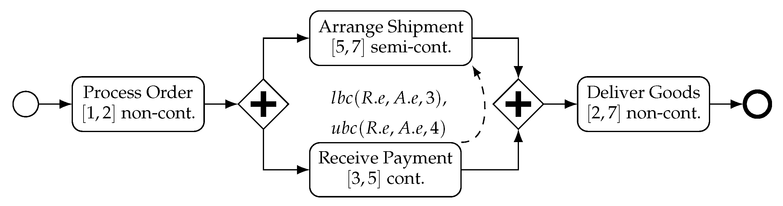
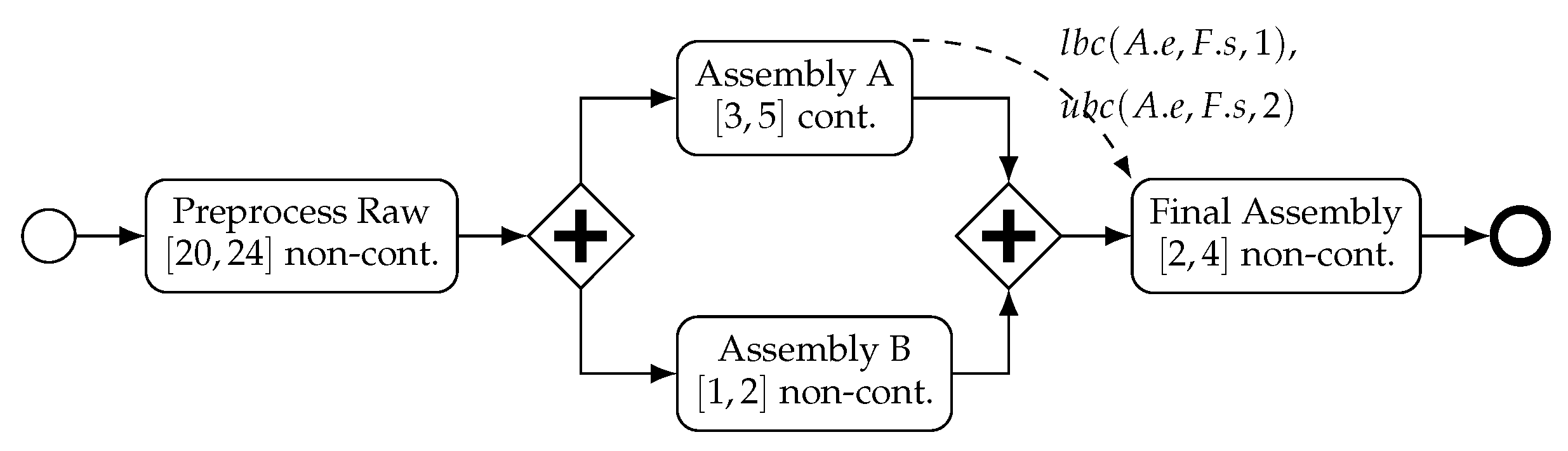
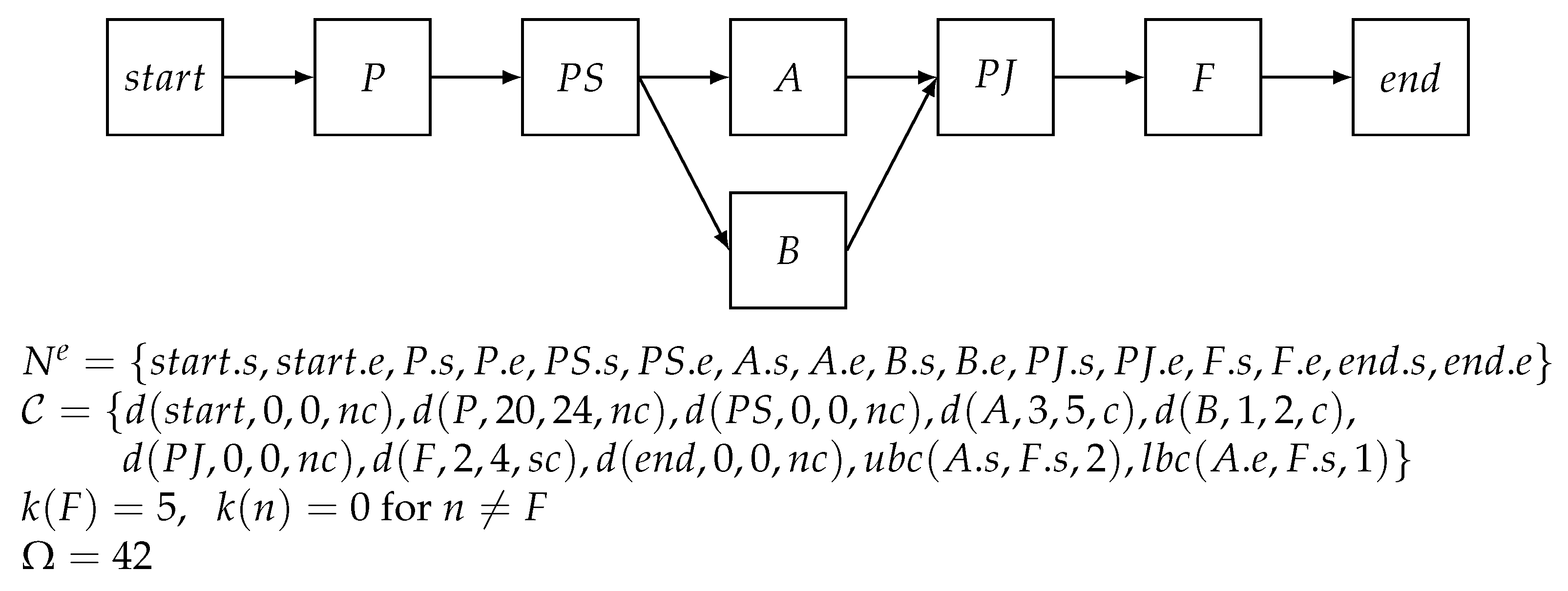
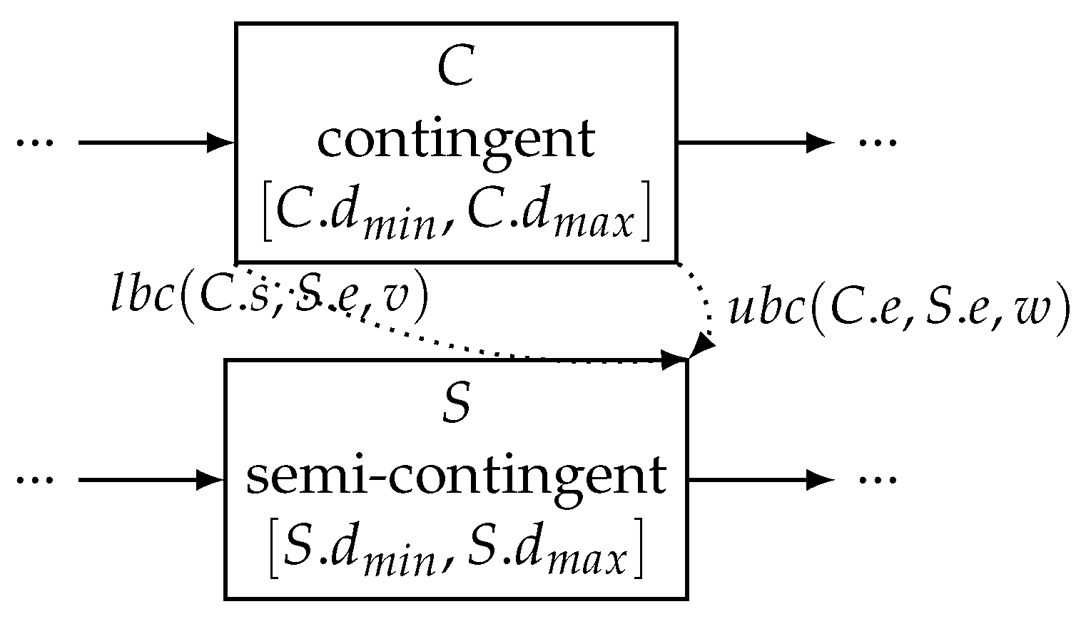
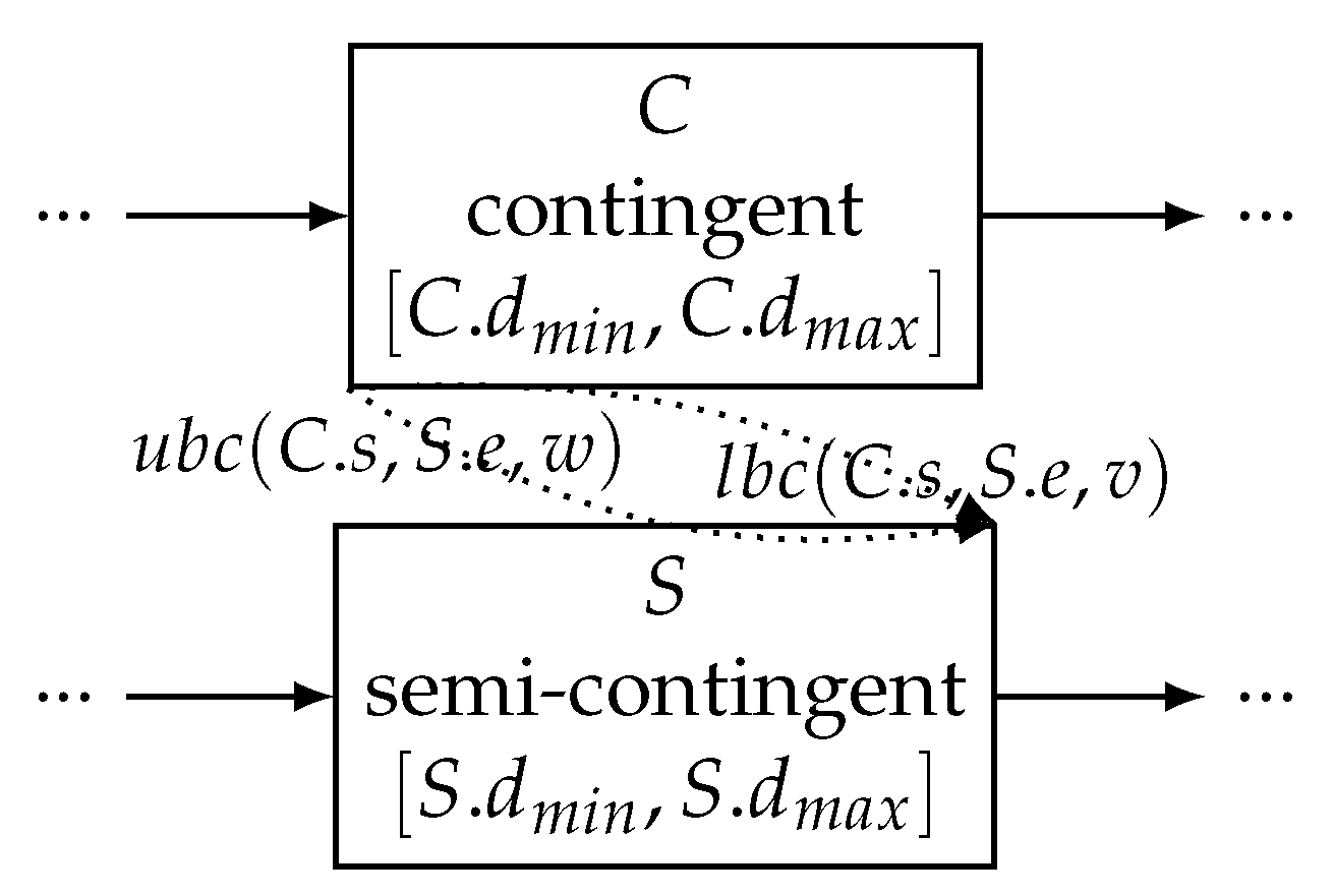
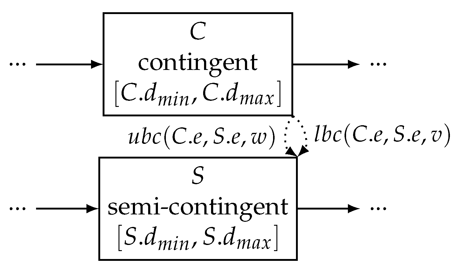
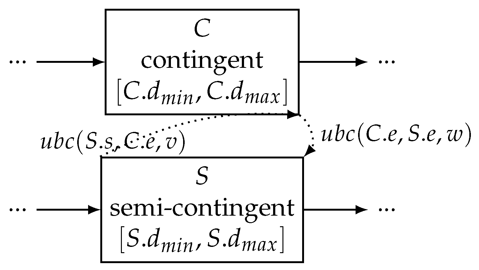
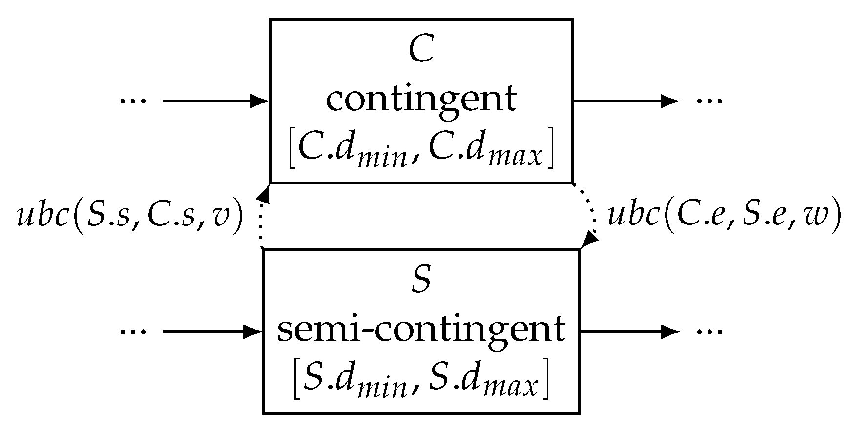
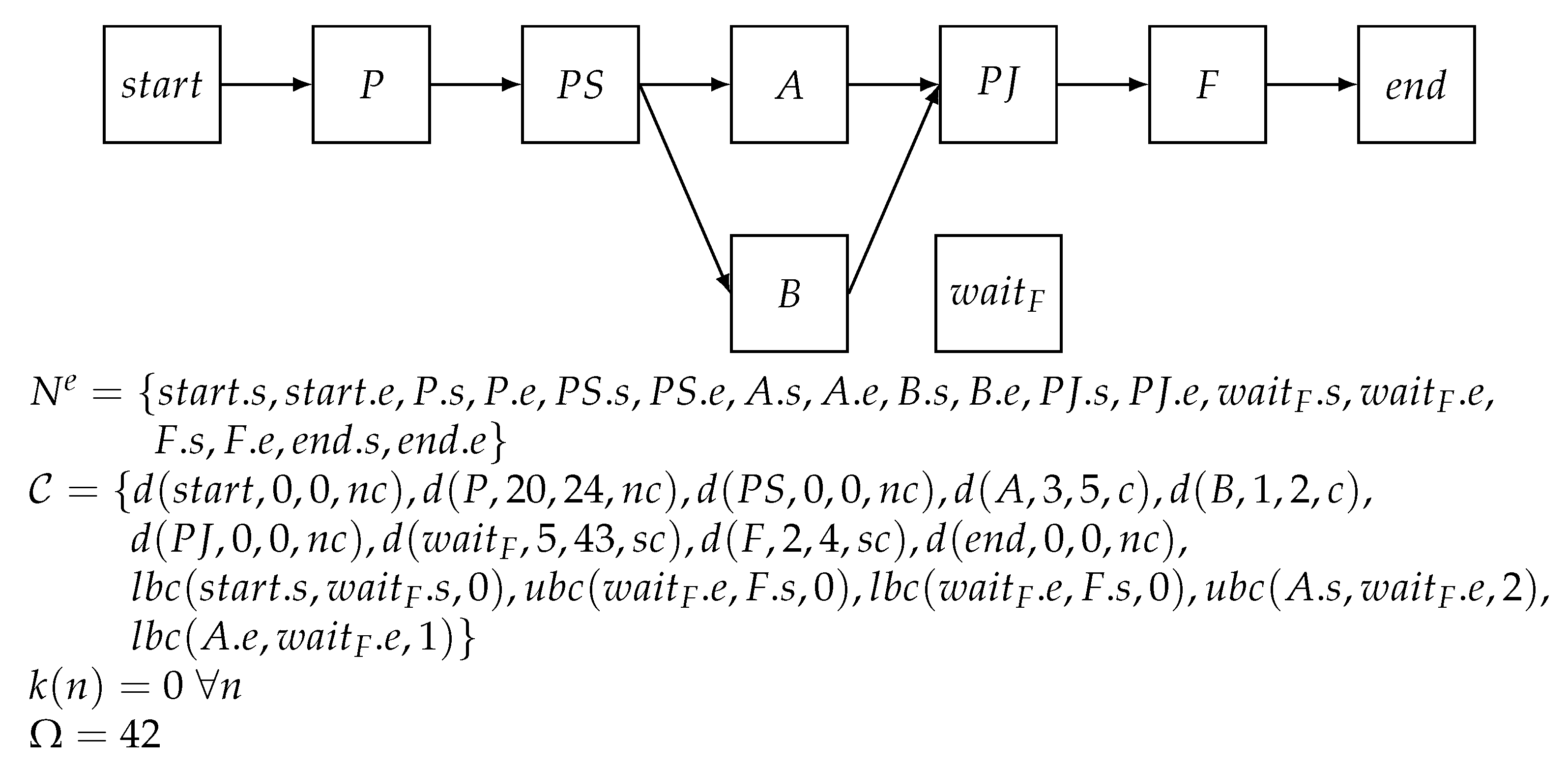
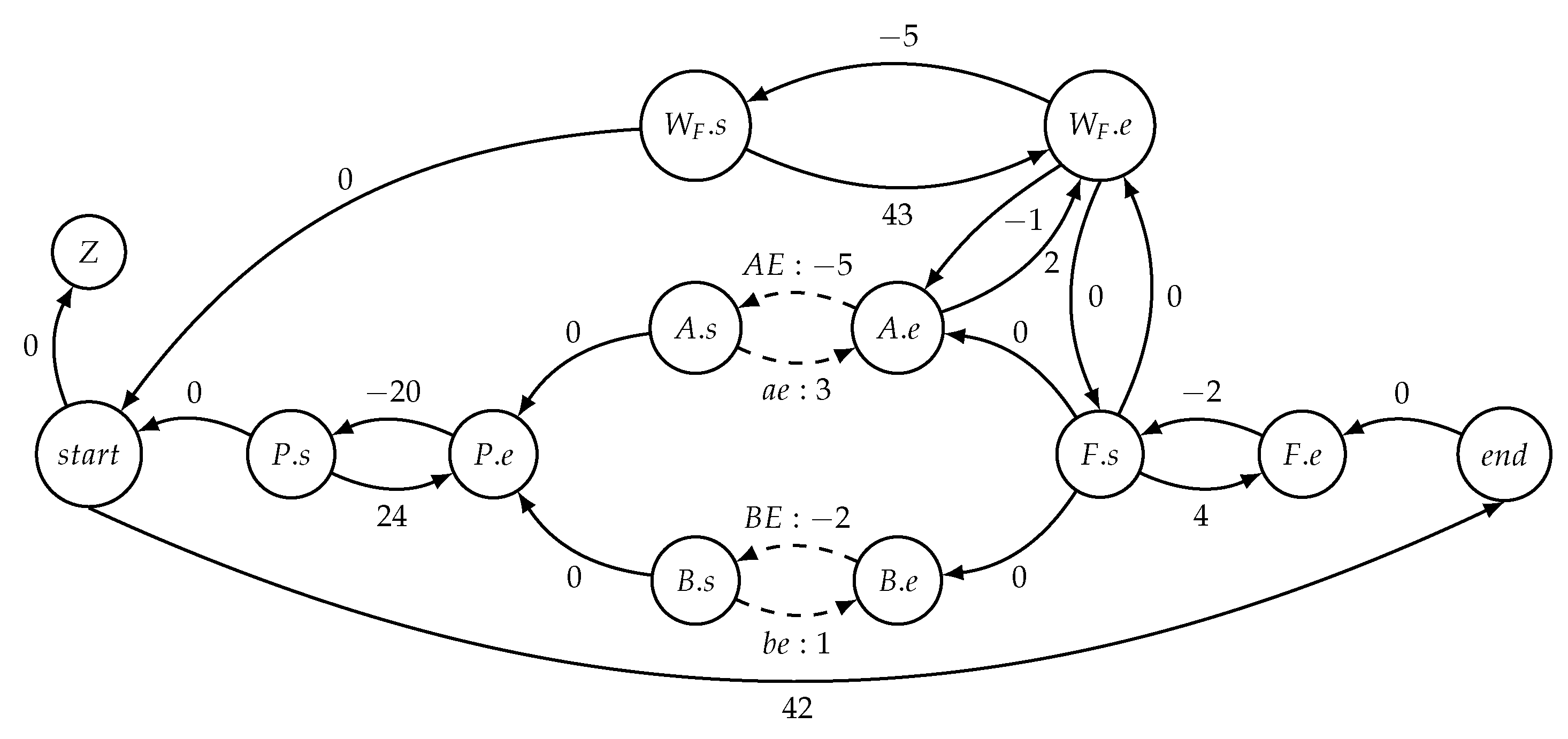
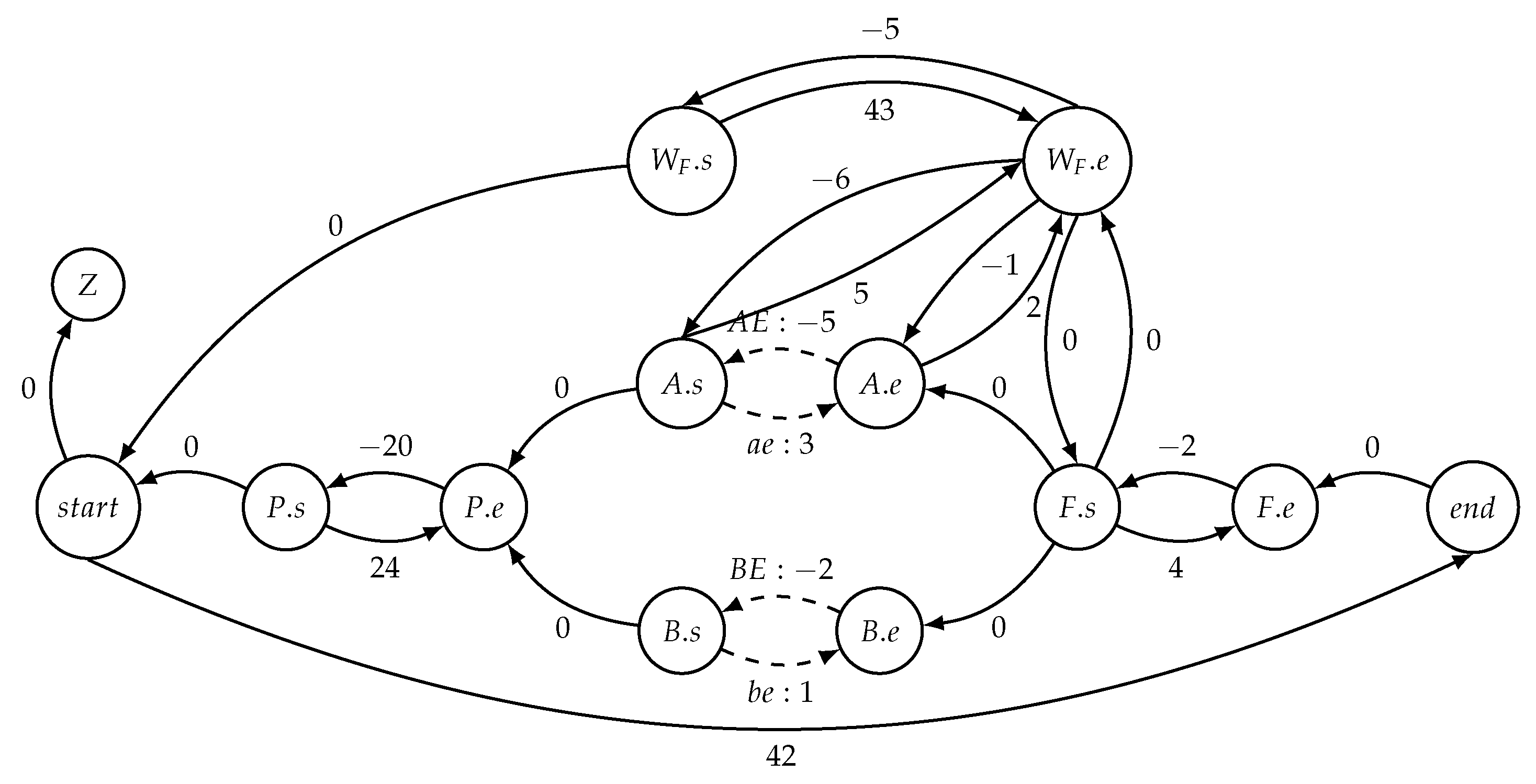
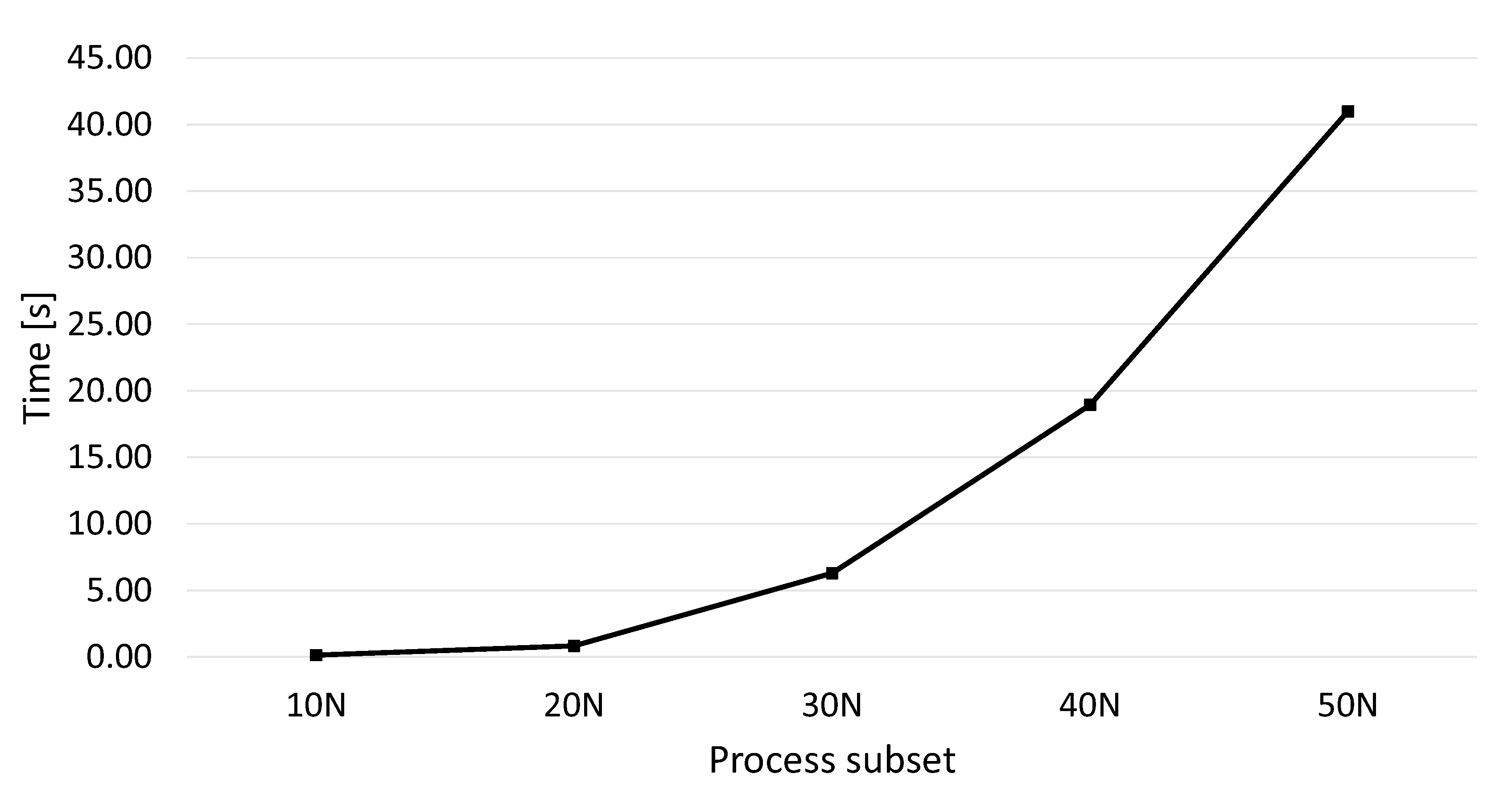
Table 1.
Sudden termination constellations, with conditions to avoid sudden termination, and constraints to add to check for semi-dynamic controllability.
Table 1.
Sudden termination constellations, with conditions to avoid sudden termination, and constraints to add to check for semi-dynamic controllability.
| Constraints | Condition to Avoid Sudden Termination | Constraints to Add |
|---|---|---|
Table 2.
Overview of the sets of processes used for the experimental evaluation. Each set contains 10 randomly generated processes.
Table 2.
Overview of the sets of processes used for the experimental evaluation. Each set contains 10 randomly generated processes.
| Subset | Min STNU Nodes | Max STNU Nodes | UBCs/LBCs | Min Splits | Max Splits |
|---|---|---|---|---|---|
| 10N | 25 | 29 | 2 | 1 | 3 |
| 20N | 45 | 51 | 4 | 1 | 4 |
| 30N | 67 | 79 | 6 | 2 | 7 |
| 40N | 91 | 107 | 8 | 4 | 12 |
| 50N | 113 | 129 | 10 | 5 | 13 |
Table 3.
Overview of the measured minimum, maximum and average times for executing Algorithm 1 on the processes of the test set.
Table 3.
Overview of the measured minimum, maximum and average times for executing Algorithm 1 on the processes of the test set.
| Subset | Min Time [ms] | Max Time [ms] | Average Time [ms] |
|---|---|---|---|
| 10N | 78 | 250 | 134 |
| 20N | 484 | 1438 | 829 |
| 30N | 4177 | 9340 | 6291 |
| 40N | 11,865 | 26,558 | 18,936 |
| 50N | 29,971 | 50,910 | 40,995 |
Publisher’s Note: MDPI stays neutral with regard to jurisdictional claims in published maps and institutional affiliations. |
© 2022 by the authors. Licensee MDPI, Basel, Switzerland. This article is an open access article distributed under the terms and conditions of the Creative Commons Attribution (CC BY) license (https://creativecommons.org/licenses/by/4.0/).
Share and Cite
MDPI and ACS Style
Eder, J.; Franceschetti, M.; Lubas, J. Dynamic Controllability of Processes without Surprises. Appl. Sci. 2022, 12, 1461. https://doi.org/10.3390/app12031461
AMA Style
Eder J, Franceschetti M, Lubas J. Dynamic Controllability of Processes without Surprises. Applied Sciences. 2022; 12(3):1461. https://doi.org/10.3390/app12031461
Chicago/Turabian StyleEder, Johann, Marco Franceschetti, and Josef Lubas. 2022. "Dynamic Controllability of Processes without Surprises" Applied Sciences 12, no. 3: 1461. https://doi.org/10.3390/app12031461
Note that from the first issue of 2016, this journal uses article numbers instead of page numbers. See further details here.