
Which Features Are More Correlated to Illuminant Estimation: A Composite Substitute


1
Faculty of Light Industry, Qilu University of Technology (Shandong Academy of Sciences), Jinan 250353, China
2
Key Laboratory of Paper Science and Technology of Ministry of Education, Faculty of Light Industry, Qilu University of Technology (Shandong Academy of Sciences), Jinan 250353, China
*
Author to whom correspondence should be addressed.
Appl. Sci. 2022, 12(3), 1175; https://doi.org/10.3390/app12031175
Submission received: 28 December 2021
/
Revised: 14 January 2022
/
Accepted: 21 January 2022
/
Published: 23 January 2022
(This article belongs to the Topic Applied Computer Vision and Pattern Recognition)
Abstract
:Computational color constancy (CCC) is to endow computers or cameras with the capability to remove the color bias effect caused by different scene illuminations. The first procedure of CCC is illuminant estimation, i.e., to calculate the illuminant color for a given image scene. Recently, some methods directly mapping image features to illuminant estimation provide an effective and robust solution for this issue. Nevertheless, due to diverse image features, it is uncertain to select which features to model illuminant color. In this research, a series of artificial features weaved into a mapping-based illuminant estimation framework is extensively investigated. This framework employs a multi-model structure and integrates the functions of kernel-based fuzzy c-means (KFCM) clustering, non-negative least square regression (NLSR), and fuzzy weighting. By comparing the resulting performance of different features, the features more correlated to illuminant estimation are found in the candidate feature set. Furthermore, the composite features are designed to achieve the outstanding performances of illuminant estimation. Extensive experiments are performed on typical benchmark datasets and the effectiveness of the proposed method has been validated. The proposed method makes illuminant estimation an explicit transformation of suitable image features with regressed and fuzzy weights, which has significant potential for both competing performances and fast implementation against state-of-the-art methods.
1. Introduction
The human vision system possess an innate “color constancy” capability, i.e., to dismount effects from the illuminant color and perceive the true color of an object [1,2]. Unfortunately, computers and imaging signal processors in vision applications do not have this capability if not to perform specific algorithms. To this end, varieties of computational color constancy (CCC) algorithms have been developed to compensate for the effects of illumination on objects’ color perception in the past decades. Once an estimated illuminant color is obtained for a captured image, the color deviation can be corrected by using the von Kries model [1,2,3]. Therefore, illuminant estimation is the key for CCC.
To date, many approaches have been proposed to estimate illuminant color by many researchers. These approaches can be roughly classified into three groups. Gray world (GW) [4,5], White patch (WP) [6], Shades of gray (SoG) [7], Gray edge (GE) [8], etc., belong to the first group—statistics-based methods, which take account of some image statistical features that are kept consistent in the image captured under canonical illuminating environments. Natural Image Statistics [9], machine learning [10], and deep learning [11,12,13,14,15,16], etc., are included in the second group—learning-based methods, which need a learning procedure utilizing various image information to pre-train models and estimate illuminant color. The third group is the combination version of the first two groups [11,17,18,19]. The unitary algorithms (i.e., the first two groups) just use a single strategy for illuminant estimation by assuming some color distribution features or learning general models from the training dataset, while the combination methods integrate the estimates from unitary algorithms into a single, final estimate. All these three groups of estimation methods usually suffer from either estimation accuracy, or computational efficiency, and result in better performances just for some specific image scenes. The overwhelming method does not appear yet.
Recently, some methods directly mapping image features to illuminant color are given rise to notice due to their simplicity and robustness [20,21,22,23]. These methods usually extract some specific features and then train a regression to capture the relationship between image features and illuminant ground truth. Although with a learning or model regression procedure, they do not need massive computation efforts and complicated model structures like deep learning. However, due to it is not clear which features are more correlated to illuminant estimation, the selection of image features for model regression remains arbitrary in the eye of the beholder. To our knowledge, there have still been no sufficient studies on how to select suitable features for the model regression of illumination estimation.
In this study, some typical image features in illuminant estimation literature are collected into a feature set. A framework with image clustering, multi-model constructing, and illuminant prediction is established to estimate illuminant color and assess the estimation performance of different features. The main contributions of this study are given as follows. (1) We develop an approach to estimate illuminant color, which includes kernel-based fuzzy c-means clustering (KFCM), optimization-based model regression, and fuzzy weighting combination. Using this method, we can easily investigate different features’ influences on illuminant estimation. (2) An optimal combination of image features is obtained by many effective experiments and analyses. Using the chosen composite feature covering a range of image characteristics as wide as possible, the performance of illuminant estimation is improved and the regression model becomes more robust. (3) KFCM and optimization-based model regression enhance the generalization ability of the proposed method; moreover, the multi-model fuzzy weighting scheme employed boosts the proposed approach to be more suitable for various image features and diverse light source characteristics.
The rest of this paper is organized as follows. Section 2 introduces the related background. The proposed method is presented in Section 3, where feature extraction, KFCM clustering, model regression, and fuzzy weighting are described in detail. Afterwards, in Section 4 many experimental results are provided to validate the proposed method, and for some remarkable issues, further discussions are given. Finally, Section 5 concludes the work.
2. Background
2.1. Imaging Model
The most commonly used imaging model for CCC is the one under the assumption of Lambertian reflection [9]. According to this model, the camera’s raw intensity response is given by [9,16]:
where c is a RGB color channel, , is a pixel location of the given image, is the wavelength of the light, is the spectrum range of the visible light, , denotes the spectral distribution of light source, denotes the surface reflectance of imaging objects, and denotes the camera sensitivity function of color channel c.
To make the problem straightforward, it is commonly assumed the image is uniformly illuminated by a single light source. Considering the case that the image scene is an ideal white surface, it yields , then the observed illuminant color will be obtained as:
Once we know , the image can be successfully chromatically adapted under the help of von Kries diagonal transformation [3]. However, with only image pixel responses given, but both and unknown, the estimation of is an under-determined issue, which needs additional assumptions to be taken.
2.2. Illuminant Estimation
This section briefly introduces the three typical methods (statistics-based, learning-based, and combinational) for illuminant estimation, and additionally, discusses some methods most related to the topic of this paper.
Statistics-based methods. These algorithms take account of certain assumptions or physical observations, and directly compute some statistical metrics of a given image to obtain the illuminant color. The advantages of these methods lie in low computational efforts, although occasionally the estimation accuracy cannot be assured. Weijer et al. [24] developed a GE framework to unify most of these algorithms, which includes n-order partial derivatives and the Minkowski p-norm given as:
where is defined as convolving the image by a Gaussian filter with scale parameter , k is a scaling, and is the estimated illuminant color. The framework is denoted as with the choices of n, p and . Some special instantiations of this framework [18,19,24,25,26] include GW (), WP (), SoG (), 1-order gray edge (GE1) (), 2-order gray edge (GE2) (), General gray world (GGW) (), etc.
Learning-based methods. In these methods, a training process is needed and then a pre-trained model is obtained to estimate the illuminant. Commonly, these methods can be further classified into two types: low-level and high-level ones [16]. The typical low-level methods are gamut mapping algorithm [27] and its extensions [28]. Other examples include some methods using probabilistic models [29], Classification-based algorithm selection [17], and machine learning algorithms [10,30], etc. Some regression-based methods [19,20,22,23] are also included in this group. These methods learn a mapping relationship between image features and illuminant ground truths from massive training data. Following the recent blooming of deep learning, high-level methods based on convolutional neural network (CNN) [11,12,14,15,16,31,32,33,34,35] have received state-of-the-art performances on various color constancy datasets. Although these methods commonly are more accurate than statistics-based algorithms, their structural complexities and computational efforts on model training hinder their applications for fast and real-time tasks.
Combination methods. Most unitary algorithms just use a single strategy that usually cannot work well for all types of images. To this end, many algorithms try to use multiple model strategies where the model set of illumination estimation is acquired from some unitary algorithms. Then by weighting the multiple estimates, a final estimate is obtained. According to whether the weights used are fixed or not, combination methods can be grouped into static weight combination and dynamic weight combination. Static weights are not suitable for diverse image features [18,36] and commonly can not ensure the robustness of illuminant estimation. Conversely, dynamic weights are more effective, but they need to tune the combination of unitary estimates against varying image features [11,17,18]. There are many examples [9,17,37,38,39] to produce the dynamic weights and find the best combination.
Related methods. In the paper [40], Zeinab Abedini provided a new explanation to some statistics-based methods from the perspective of the percentage of pixels involved in illuminant estimation. In these methods, all pixels equally attend in illuminant estimation (e.g., GW), or some pixels are radically selected for processing and the others are ignored (e.g., WP, Bright Pixel [41], PCA-based method [21], Gray Pixels [42], Gray Index [43]). Naturally, the explanation can be extended as a weight-based technique, i.e., all pixels are used, but the weights for different pixels are not the same. And, the weights can be implicitly or explicitly presented. GGW, GE, and SoG are included in this explanation since they can be explained to have implicit weights with the structure of the p-th Minkowski norm. Local surface reflectance (LSR) [44] which uses WP to weight GW can also be seen to have implicit weights [40]. According to this explanation, illumination estimation becomes the regression function of the pixels distribution features and the corresponding weights. Similarly, in learning-based methods, some direct regression-based methods have been proposed [20,21,23,40,45] in recent years, which simply map image features to illuminant. One of the remarkable methods is based on the Corrected Moment (CM) [20]. The CM-based method provides an efficient methodology to yield the illuminant estimation using a polynomial regression from multiple low-level-based methods. Other techniques, e.g., regression tree [30], fuzzy logic [19], deep learning [46,47], also can be regarded as regression-based methods with complex structures. Although these algorithms can achieve outstanding performances, their disadvantage is that they make illuminant estimation work in a black box without further considering the specific features of different images. These methods can be improved if the regression or weighting model is adjusted with image intrinsic features. So it is very important to assess the impacts of selected image features on illuminant estimation and determine which features are more correlated to illuminant estimation. The optimal combination of selected features will make illumination estimation regression more efficient.
2.3. Color Correction
For a given image, once the illuminant color is estimated as a illumination vector , the image should be corrected by the von Kries diagonal transformation [3]. All the colors of the color-biased image under the unknown light source (u) should be mapped to the colors under a canonical illuminant (c), which is demonstrated as follows:
where and denote the image colors under the unknown light source and a canonical illuminant, respectively.
3. Proposed Method
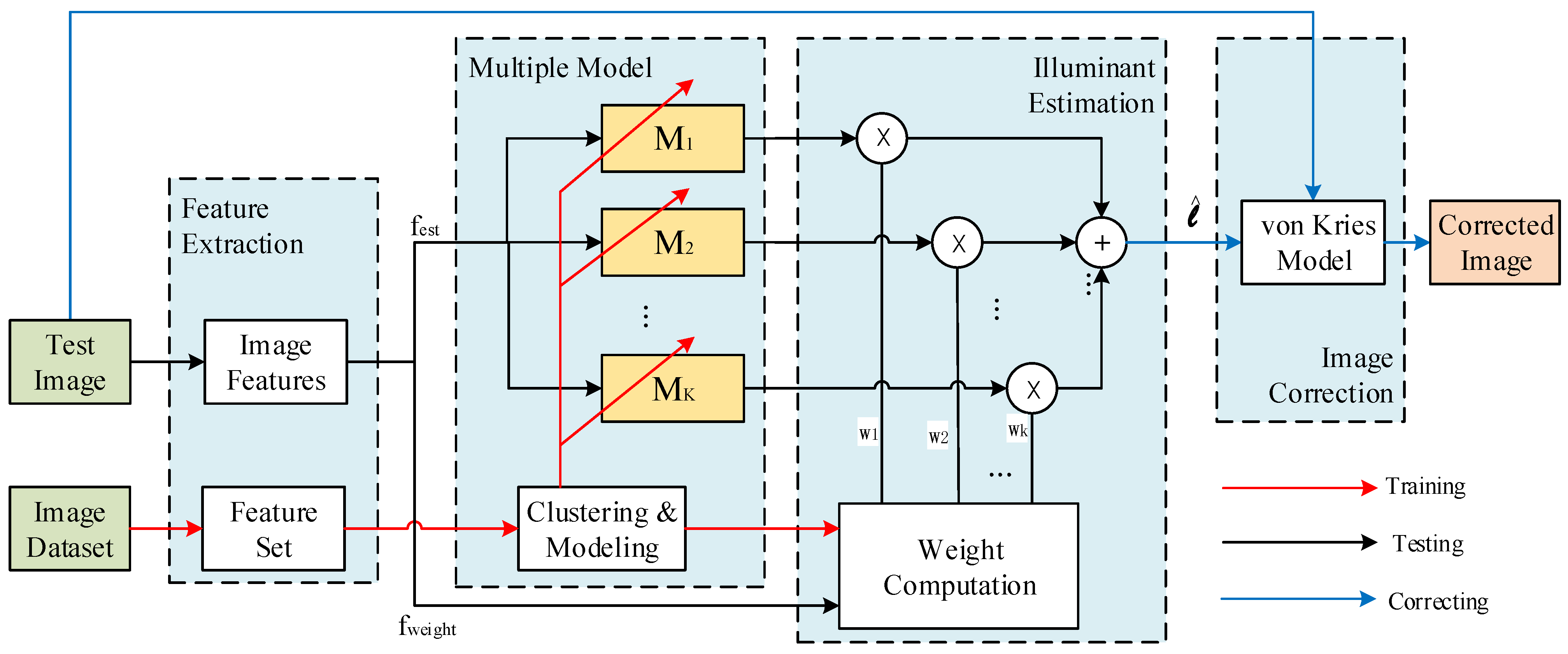
In the proposed method, illuminant estimation is achieved by a serial of linear or nonlinear transformation of suitable image features. The proposed method also can be easily used to assess the illuminant estimation performance by utilizing different features to construct more efficient feature substitutes. The flowchart of the proposed framework is illustrated in Figure 1.
In the training phase, the training dataset is classified into different clustering using the KFCM algorithm. For each cluster, the illuminant estimation models are obtained using a non-negative least square regression (NLSR) method. For a given test image that has been removed dark level and saturation level in the linear RGB space, the corresponding image features will be extracted and then the final estimated illuminant will be produced by fuzzy weighting all outputs of multiple regression models.
3.1. Features Extraction
The image features can be used as representatives of an original image, just with a compact data length. Since it is not clear which features will affect the illuminant estimation much more, in this paper a series of features are gathered into a candidate set to explore the suitable feature selections and better illuminant estimation. The features in the feature set are derived from the up-to-date literature that provides some effective learning-based methods of illuminant estimation. These features are low-level, or middle-level [38]; here we do not use high-level or semantic features, since semantic features are commonly specific to different images and may have small effects on illuminant estimation [38]. Several image features are extracted for each image as follows.
Corrected moments (CM) [20,48]. They are the polynomial expansions of the 2nd, 3rd, and 4th degree, which are described by the following vectors:
Here r, g, and b are the illuminant components estimated by some general methods, such as GW, SoG, etc. According to the above expressions, the element numbers recorded in a CM feature are 9, 19, and 34, respectively.
RGB-uv histogram (RGBuv). The paper [49] extracted a histogram from the log-chrominance space to represent the bulk of information in a color image. This feature is called RGB-uv histogram, which describes the color distribution feature of an image as a tensor. The works in [49] have validated the effectiveness of this feature to illuminant estimation. To short the length of this feature, a PCA-based dimensionality reduction step is applied to get a compact representation for each RGBuv histogram. As a result, the RGBuv of any image I can be expressed by a serial of primary component coefficients :
where p is the number of primary components, and .
Color moments (ClrM) can characterize the color distribution in an image. Commonly, three central moments, i.e., first-order moments (Mean), second-order moments (Standard deviation), and third-order moments (Skewness), are sufficient to express the main color distribution of an image. Considering the size of image, each image is evenly divided into 3 × 3 sub-blocks in this study; therefore, 81 moments for an image I can be obtained if the moments are calculated for each RGB channel:
Cheng’s simple features (ChengSF) [30]. These features are a group of intensity-invariant features based on normalized chromaticity. There are four color chromaticity features extracted from an image, i.e., average color chromaticity , brightest color chromaticity , dominant color chromaticity , and chromaticity mode of the color palette . Here r and g are the normalized chromaticity components of RGB color [30]. For an image I, ChengSF can be expressed as follows:
Color distribution features (CDF). In paper [19], Luo proposed a compact color distribution feature for illuminant estimation, which is a combination of the number of image colors , chromaticity features in Equation (10), and color moments in Equation (9). For an image I, the obtained CDF vector is as follows:
where the two adjustable factors, and , control the influences of different components on the illuminant estimation.
Initial illuminant features (IIF). In paper [19], some unitary algorithms, i.e., GW, WP, SoG, GE1, GE2, GGW, PCA, and LSR, are applied to get eight initial illuminant estimates for an image. These initial estimates are integrated into a vector, i.e., IIF, as a metric of illuminant characteristics. For an image I, the IIF vector is expressed as follows:
where is defined as the Euclidean distance between initial illuminant estimates and .
3.2. KFCM Clustering
In the training stage, a better classification can achieve the appropriate divisions of the training dataset. In each division the features will be close each other and fit for illuminant modeling. We use some above-mentioned features to classify the training dataset by the KFCM method.
KFCM is derived from fuzzy c-means (FCM). FCM is a classification algorithm based on fuzzy sets, which results in clustering partitions with the maximum similarity among samples in the same cluster, while the minimum similarity among different clusters [50]. As an improved version of the common c-means algorithm, FCM provides flexible fuzzy partitions since the training samples are clustered in terms of the membership functions. For the standard FCM, a cost function based on the Euclidean distance is minimized to solve the cluster centroids and the membership degrees of all samples:
where is the Euclidean norm to measure the similarity between sample data and cluster centroid; is the degree of membership for the sample in the cluster i, ; is the centroid of the cluster i, ; n is the total number of samples; m is the exponent of the membership; and c is the cluster number. Furthermore, a kernel function can be introduced into FCM by a nonlinear mapping , which maps the low dimension vector x into a high dimension space. Then the kernel-based FCM, i.e., KFCM, is to minimize the following cost function:
where
Here is an inner product kernel function, and . In this study, we adopt the Gaussian function as a kernel function, i.e., , where is the kernel width; then we can get and . According to Equation (15), Equation (16) can be rewritten as:
From Equation (16), we can see that the cost function is minimized when the first-order partial derivatives with respect to and both are zeros. By these two necessary conditions, the final clusters and their centroids are iteratively obtained as follows:
Here , and .
It is worthy to mention that the clustering performance of KFCM will be influenced by different kernel functions and their parameters. Although the results of Equations (17) and (18) are deduced using the Gaussian kernel function, other kernel functions just satisfying also can be used here. In the Gaussian kernel function, the kernel width is commonly used as the key tuning parameter. Due to the Gaussian kernel being a typical local kernel function, the function value is largely affected by the data closer to the test point. Hence we can determine the kernel width according to the average distance between the sample data and the cluster centroid. This will ensure that the data in the same cluster play a dominant role in the corresponding kernel function values, while the data out of this cluster make a slight impact on the corresponding kernel function values. In additions, different from single-model methods, multi-model ones used in this study can select different kernel parameters for different clusters.
3.3. Model Regression
In this study, to avoid complicated structures of deep neural networks, we just employ the least-square-based method since we focus on finding more suitable features for illuminant estimation rather than aiming for high performance. The precision of model regression is sacrificed somewhat, but the speed and robustness of illuminant estimation can be attained substantially.
We construct the regression relationship directly from image features to illuminant ground truths as follows:
where is the vector of illumination ground truths of the training samples, M is the regression model matrix, and is the feature matrix of all sampling images. In general, we obtain the solution of Equation (19) as , where is the Moore-Penrose inversion of the feature matrix . But some elements in the resulting M might be negative, which may deteriorate the robustness of the model. To address this problem, we seek the solution to minimize with each element in M no less than zero. Therefore, we can train a regression model to minimize the -norm loss between the reconstructed and ground truth illumination by solving the non-negative least square problem:
Therefore, for all partitions of the training set from KFCM, we can get a series of models and construct a model set as follows:
where K is the number of the obtained multiple models for the training dataset.
3.4. Fuzzy Weighting
For a test image , the final output of the illuminant estimation is synthesized by fuzzy weighting the outputs of all models, which is given as:
where is the weight of the i-th model , and denotes the extracted features of the test image . For an image sample in the training set, is known (it is the membership of degrees for this sample); while for a new test image not included in the training dataset, is needed to be computed by determining what degree the test sample belongs to each cluster obtained via KFCM. That is to say, all possibilities that an image falls into each cluster should be acquired by calculation. To this end, we define a variable as the squared Euclidean distance between the test image’s feature vector f and the cluster centroid , . Then a radial basis function is constructed to represent the probability for the test image belonging to the cluster i:
where denotes the radial fall-off factor. In this way the weights are obtained, and the illuminant color of the test image can be predicted by Equation (22).
4. Experimental Results
4.1. Experimental Set-Up
Dataset. The proposed framework should be verified on a mass of image examples that have a wide scale of color distributions and diverse illuminant characteristics. In this study, the two datasets (Gehler-Shi [51] and Cube+ [15,52]) are employed as the training and testing datasets. Both datasets are suitable for the evaluation of illumination estimation algorithms due to they include typical real-world images with varieties of illumination. In each image of the Gehler-Shi dataset, there is a color-checker board added into the lower right corner for calculating the ground truth illumination, while in the Cube+ dataset, a SpyderCube color target is used in each scene for the same purpose. These color-checker boards and color targets are masked when the images are utilized in the procedures of our experiments. The proposed method performs the standard 3-fold cross-validation for the training and testing procedures, which is commonly used in existing learning-based illuminant estimation literature.
Implementation details. We conducted three types of experiments to test our proposed approach, i.e., (1) Experiment A, training and testing on an individual image dataset from different cameras; (2) Experiment B, training and testing on an image set from an identical camera; and (3) Experiment C, training and testing on different image datasets or a combination of several image datasets. Since an image from a certain camera or dataset might contain some unique information of this camera or dataset, it is necessary to perform Experiment A and Experiment B. Both experiments will help to investigate on selecting suitable features of illuminant estimation for our method under the circumstances ruling out the influence of camera or dataset. On the other hand, considering the training/testing across datasets is the most common situation for learning-based illuminant estimations, Experiment C is employed to validate our method’s effectiveness on a combination of multiple datasets.
Our MATLAB implementation is shown in https://github.com/yunhuiluo/if2ic (accessed on 28 December 2021). In the training stage, the training dataset will be clustered according to the selected image features and the regression models will be constructed for each cluster. Since the classification algorithm based on KFCM is not complex mathematically, it takes a very short time compared with other learning methods like deep learning. For example, it requires approximately 12.6 seconds for classification and training 6 models for the Cube+ dataset. Once the training is finished, the illuminant estimation process costs an average time of 0.93 seconds for a new test image with pixels, 48 bits depth, and PNG format; this process includes feature extraction, multiple model estimation, weight computation, and fuzzy weighting output. All the runtimes above-mentioned were obtained from a laptop computer with an Intel Core i5-2450M @ 2.50 GHz CPU.
By default, we set the cluster number when using the combination of Gehler-Shi and Cube+, and we set the fall-off factor mentioned in Section 3.4. We utilize the KFCM algorithm to perform image clustering based on the features of IIF, and set the kernel width to be 140. Our method requires 6.7 MB to store the classification parameters, multiple model matrix, and some configurations. In our experiments, each PCA feature vector was also represented by 53 primary component scores (the same with [49]) for any RGBuv feature. Since each time the cluster iteration of KFCM algorithm begins from some random initial center positions, the performances for each experiment with the same configurations might be tinily different.
Evaluation Metrics. The two performance metrics widely used in color constancy literature are employed in this paper. The first one is recovery angular error (recovery AE) [9,18], which is defined as the angle in degrees between the illumination’s actual 3D-chromaticity and its estimated 3D-chromaticity : Here the symbol of · denotes the scalar product (dot product), and the symbol of indicates the Euclidean norm of a vector. The second metric is called reproduction angular error (reproduction AE) [53,54], which usually is more efficient than the traditional recovery AE. The reproduction AE is defined as the angle in degrees between the true color of white surface and the reproduced color of white surface: . Here denotes the white light source (true color of white surface), , and indicates the reproduced color of white surface, , which is the actual 3D-chromaticity divided by the estimated 3D-chromaticity .
Since both recovery and reproduction AEs are not normally distributed, the Mean and Median values along with the Trimean value are used to assess the statistical performance of color constancy algorithms in this study. Trimean is defined as a weighted average , where , , and are the first, second, and third quantiles of recovery or reproduction AE, respectively. In addition, the maximums of both AEs are used as extra metrics to assess the robustness of the illuminant models along with the metric of .
4.2. Experiment A: Individually Testing on Different Datasets (Within Dataset)
In this experiment, our method is independently applied to different datasets. Table 1 and Table 2 compare some performance metrics between our method and some conventional algorithms on the Gehler-Shi dataset and the Cube+ dataset, respectively. In order to illustrate the impacts of different features on illuminant estimation performances, all types of features given in Section 3.1 are investigated using the proposed method.
Table 1 shows that our results (except for the one using CDF features) outperform most unitary algorithms on the Gehler-Shi dataset. For example, the Mean of recovery AE is 4.66 for GGW, and 4.17 for our method using ChengSF; The Trimean of recovery AE is 3.81 for GGW, and 3.41 for our method using ChengSF. There is a significant performance improvement near 10% from GGW to our method using ChengSF. Table 1 also shows that our method with some combined features (i.e., RGBuv+ChengSF, RGBuv+ChengSF+IIF, and RGBuv+ChengSF+IIF+) is superior to some learning-based methods, e.g., Bayesian [29], Natural Image Statistic [46], and WCS with partitioning [40], etc. What’s more, we can notice that the proposed method with the combined features is better than most previous methods in terms of the metrics of Best 25% and Worst 25%. This validates that the proposed method can achieve a outstanding illuminant estimation regardless of image features.
Table 2 gives the results for the Cube+ dataset. Most metrics of our results in Table 2 are better than those in Table 1, since the Cube+ dataset contains more images than the Gehler-Shi dataset. It can be seen that the statistics of our method with the combined features are almost all better than one of learning-based methods—Attention CNN [56]. These results further indicate the proposed method is effective to achieve a better regression accuracy using optimally selected feature combinations. It should be noticed that the composite features of RGBuv+ChengSF+IIF can obtain outstanding performances using our method. More comparisons of statistical metrics are provided in our GitHub repositories.
4.3. Experiment B: Testing on Image Set from Identical Camera (Within Camera)
This experiment uses some images from an identical camera as the training and testing data, which is to verify the estimation accuracy within the camera using the proposed method. Table 3 and Table 4 compare the performance metrics for some conventional methods and our method with different features within an identical camera. Here Canon 5D is one of the cameras used by the Gehler-Shi dataset, and Canon EOS 550D used by the Cube+ dataset, respectively. For Canon 5D, 482 images are picked out from the Gehler-Shi dataset, and for Canon EOS 550D, 853 images are randomly selected from the Cube+ dataset. The standard 3-fold cross validation is independently applied to the constructed datasets to train and test the proposed method.
Table 3 and Table 4 show that the proposed method using image feature regressions achieves better performances than some traditional methods such as WP, GW, PCA-based, LSR, etc. Using the individual feature in the proposed method, the feature of RGBuv receives the best results. According to the discussion in the paper [49], the RGBuv feature can effectively cover the color distribution of an image. The results in Table 3 and Table 4 also validate this viewpoint. It can be seen that compositing several features will provide better results, e.g., RGBuv+ChengSF, RGBuv+ChengSF+IIF, and RGBuv+ChengSF+IIF+. For the camera of Canon 5D, the composite of RGBuv+ChengSF+IIF has a 25.9% performance improvement in recovery AE Mean, and a 25.4% performance improvement in recovery AE Trimean, compared with WP. For the camera of Canon EOS 550D, the same improvements reach 42.3% and 32.3% (ours versus GGW), respectively. In our experiments, the optimal feature combination is RGBuv+ChengSF+IIF, which obtains outstanding performances compared with other feature selections.
The combination of image features affects the illuminant estimation since the proposed method is to directly map the extracted features to illuminant color. Except for the results listed in Table 3 and Table 4, we conducted many other experiments for the proposed method with more feature combinations. We find that it is not the more combined features the better performance. Just the correlated features are effective for illuminant estimation. Thus, it is significant to find which features are more correlated to the illuminant estimation. In this study, we just investigated several features and their combinations. From the experimental results given, there are reasons to believe that if we find more effective features, the performance can be even more improved by the proposed method.
4.4. Experiment C: Cross-Dataset, Cross-Camera Testing
To investigate the robustness of the proposed method, some cross-dataset testing should be performed on multiple datasets. In this experiment, the combination dataset of Gehler-Shi and Cube+ is used by these testing through the 3-fold cross-validation technique. Table 5 provides the statistical metrics of the experimental results.
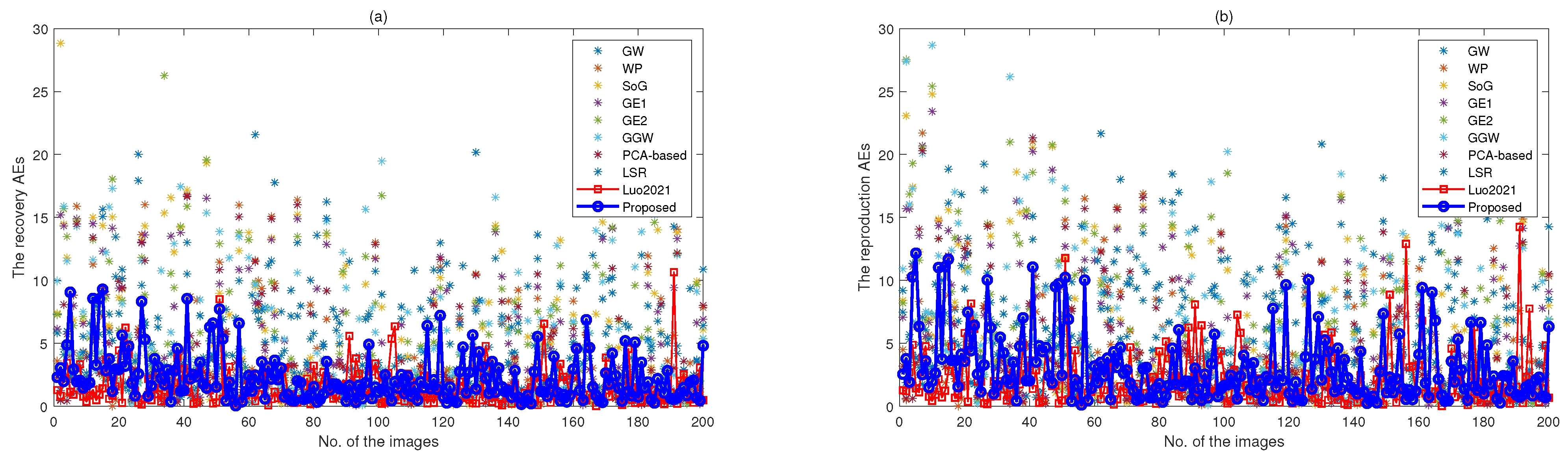
Since the combined dataset can cover a wider range of image features and illuminant regions, the classification and models obtained by the proposed method commonly receive better generality on illuminant estimation. Table 5 validates this viewpoint. It can be seen that the obtained statistical metrics for all images in the Gehler-Shi and Cube+ datasets reach the good performances, e.g., the Mean and Maximum of recovery AE respectively are 2.13 and 14.83 for the selected optimal features of RGBuv+ChengSF+IIF. Figure 2 shows the recovery and reproduction AEs’ distribution for some images from the Gehler-Shi and Cube+ datasets using some conventional methods and the proposed method. These results indicate the proposed method can work well and reach excellent performances. It should be pointed out that the selected optimal features of RGBuv+ChengSF+IIF are prerequisites for these results.
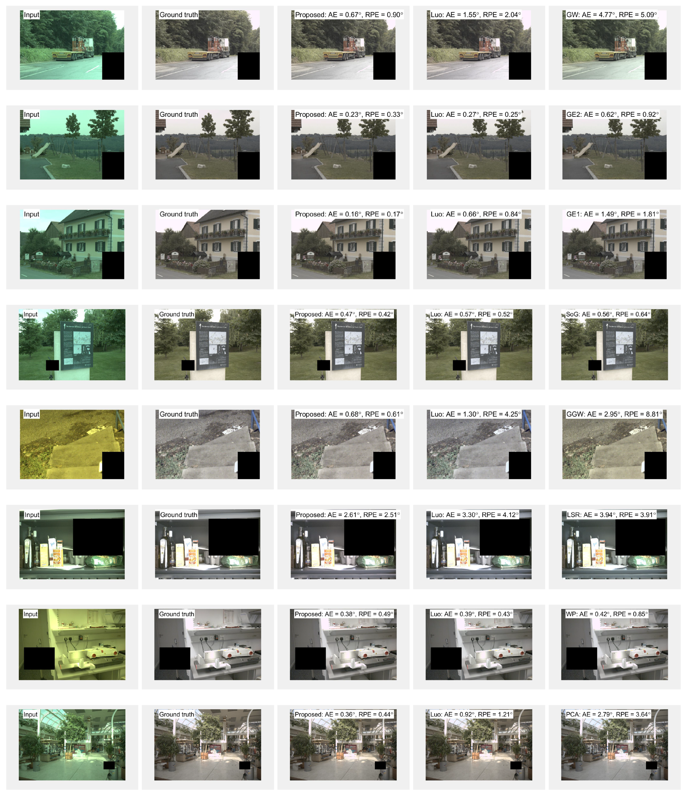
In real life, photographers usually cannot capture images under perfect or standard illumination. A complex lighting environment results in changing brightness and contrast. A robust color constancy algorithm should be able to deal with these challenges. Our algorithm essentially is a weight-based method in which the features more related to illuminant color are highlighted and used to deduce dynamic weights. Figure 3 shows some visual results to face some challenging image scenes. As shown in this figure, our algorithm with the feature combination of RGBuv+ChengSF+IIF reaches the better performance compared with some conventional methods. Consequently, the proposed method has the great potential to color constancy of a wide range of images. For more examples, please refer to the related materials at our GitHub repositories.
4.5. Additional Experiments
In the proposed method, many factors will affect the performances of illuminant estimation. Some experiments are conducted to explore these influences.
Clustering methods and cluster numbers. For the proposed method, we perform KFCM clustering by default to classify the training data. For comparisons, the other two clustering algorithms, i.e., K-means and the two-step method [19], are also added to the proposed framework. The reason for selecting K-means and the two-step method is that the former is one of the most commonly used clustering methods, and the latter is an effective algorithm of color constancy based on cluster models. For each clustering algorithm, we can manually set different cluster numbers in order to obtain better results. Table 6 gives some statistical metrics using different clustering methods and cluster numbers. Comparing the results using different configurations, it can be seen that the proposed method along with KFCM seems to be more effective than using K-means and the two-step method. One of possible reason might be that KFCM can provide flexible division for the training set, which enhances the robustness and generalization of the proposed method. And we find or 5 is the appropriate selection for our method under the KFCM clustering on the combination dataset of Gehler-Shi and Cube+. It is natural that the cluster number should increase for better modeling performance if we use another dataset with more image samples.
Kernel width of KFCM. In the proposed method, kernel width will affect clustering divisions, which will result in different performances. Table 7 provides some statistical metrics on the Gehler-Shi and Cube+ datasets to show the influences of kernel width in KFCM clustering. We can find that the optimal choice of kernel width for our experiments is ~180. Commonly, the optimal values are obtained by trial and tried in various testing. It should be noticed that the optimal kernel width is varying with the training dataset. Therefore, as an option, Particle Swarm Optimization can be used to search for the optimal kernel width.
4.6. Discussion and Analysis
In this paper, the experimental results show that the performances of the proposed method are on par with many statistics-based and learning-based approaches. And we have tentatively identified the feature combinations that are more correlated to illuminant estimation based on a specific feature set. In the meantime, we can obtain some useful observations.
(1) The methods based on composite features generally work better than most methods based on unitary features. The key to the combination of features is to find a compact presentation to cover a much wider range of image features and illuminant characteristics. The dimension of the features is not an obstacle; if the feature dimension is low with useful information compressed, we can use different kernel functions to map them into a higher dimension space [20,48]; on the contrary, if the dimensionality is high with much redundant information, we can use the PCA technique to reduce the dimensionality of the features [49]. To date, as it were, the trial-try method by experiments is still the major route to construct artificial features for regression models of illuminant estimation. Thus, choosing an appropriate feature combination is significant to accurate and robust illuminant estimation.
(2) The methods based on feature regression clearly depend upon not only the optimal feature combinations but also the scale and characteristics of the training sets. If the training examples are from an identical camera or a benchmark dataset using multiple cameras while the testing example is taken from the same camera or dataset, the illuminant estimation accuracy is usually very high. However, if training images from a certain camera or dataset using multiple cameras while the testing example from other camera or dataset, i.e., cross cameras or cross datasets, the illuminant estimation accuracy is commonly worse than expected. As the scale of the training dataset increases and the illuminant range of the training sets extends, a single model is not a preferred option for regression modeling. So a multiple model strategy with high efficient classification (or clustering) becomes preferred, like KFCM clustering and regression modeling associated with fuzzy weighting in this paper.
(3) The type of feature, i.e., features from different cues, generally affects and limits the performances of illuminant estimation. In this paper, we just considered two types of features (low-level CDF and middle-level IIF [18,38,58]. We found the performance improvement is limited although we seem to have an optimal feature combination. High-level scene category or semantic features, e.g., Weibull parameters with content-based features [17], 3D scene geometry [37], indoor/outdoor classification [59], etc., can also be exploited in the proposed method.
5. Conclusions
For the regression-based illuminant estimation methods, it is uncertain which features are more efficient to regress illuminant color. In this research, a flexible framework is developed to integrate KFCM, NLSR, and fuzzy weighting, which can result in outstanding performances of illuminant estimation. By extensive experiments with a series of artificial features weaved into this framework, to some extent it is clarified which features are more correlated to illuminant estimation. Moreover, we exploited an optimal feature combination based on the given feature set, which obtains a significant performance improvement for illuminant estimation.
The proposed method and its framework can be used to test and compare the influences of image features on illuminant estimation. From this, we can optimally deploy the appropriate image features for illuminant estimation in a more objective way, rather than in an empirical, arbitrary manner. If the feature sets contain more feature candidates, the performance of illuminant estimation is expected to be further enhanced.
This study focuses on determining which features are more correlated to illuminant estimation in a limited feature set. Therefore, more related image features, including high-level semantic features, can be further taken into account. Besides, considering there are different intrinsic and implicit cues for different camera sensors, pre-selecting images in terms of camera sensor characteristics and then constructing multiple models may be another pathway to improve the proposed method.
Author Contributions
Conceptualization, Y.L. and X.W.; methodology, Y.L.; software, Y.L.; validation, Y.L., X.W. and Q.W.; formal analysis, Y.L.; investigation, Y.L.; resources, Y.L.; data curation, Y.L. and X.W.; writing—original draft preparation, Y.L.; writing—review and editing, Y.L. and X.W.; visualization, X.W.; supervision, Y.L.; project administration, X.W.; funding acquisition, Q.W. and Y.L. All authors have read and agreed to the published version of the manuscript.
Funding
The Project Supported by the Foundation (No. KF201603 and ZR202001) of Key Laboratory of Paper Science and Technology of Ministry of Education of China.
Institutional Review Board Statement
Not applicable.
Informed Consent Statement
Not applicable.
Data Availability Statement
Not applicable.
Conflicts of Interest
The authors declare no conflict of interest.
Abbreviations
| CCC | Computational color constancy |
| GW | Gray world |
| WP | White patch |
| SoG | Shades of gray |
| GE | Gray edge |
| GGW | General gray world |
| PCA | Primary component analysis |
| LSR | Local surface reflection |
| CM | Corrected moments |
| CDF | Color distribution feature |
| IIF | Initial illumination feature |
| KFCM | Kernel fuzzy c-means clustering |
| NLSR | Non-negative least square regression |
References
- Barnard, K.; Cardei, V.C.; Funt, B.V. A comparison of computational color constancy algorithms. I: Methodology and experiments with synthesized data. IEEE Trans. Image Process. 2002, 11, 972–984. [Google Scholar] [CrossRef] [PubMed]
- Barnard, K.; Martin, L.; Coath, A.; Funt, B.V. A comparison of computational color constancy algorithms. II. Experiments with image data. IEEE Trans. Image Process. 2002, 11, 985–996. [Google Scholar] [CrossRef] [PubMed] [Green Version]
- von Kries, J. Influence of adaptation on the effects produced by luminous stimuli. In Sources of Color Vision; MacAdam, D.L., Ed.; The MIT Press: Cambridge, MA, USA, 1970; pp. 109–119. [Google Scholar]
- Buchsbaum, G. A spatial processor model for object colour perception. J. Frankl. Inst. 1980, 310, 1–26. [Google Scholar] [CrossRef]
- Provenzi, E.; Gatta, C.; Fierro, M.; Rizzi, A. A spatially variant white-patch and gray-world method for color image enhancement driven by local contrast. IEEE Trans. Pattern Anal. Mach. Intell. 2008, 30, 1757–1770. [Google Scholar] [CrossRef]
- Land, E.H. The retinex theory of color vision. Sci. Am. 1977, 237, 108–128. [Google Scholar] [CrossRef]
- Finlayson, G.D.; Trezzi, E. Shades of gray and colour constancy. In Proceedings of the Twelfth Color Imaging Conference: Color Science and Engineering Systems, Technologies, Applications, CIC 2004, Scottsdale, AZ, USA, 9–12 November 2004; pp. 37–41. [Google Scholar]
- van de Weijer, J.; Gevers, T.; Gijsenij, A. Edge-based color constancy. IEEE Trans. Image Process. 2007, 16, 2207–2214. [Google Scholar] [CrossRef] [Green Version]
- Gijsenij, A.; Gevers, T. Color constancy using natural image statistics and scene semantics. IEEE Trans. Pattern Anal. Mach. Intell. 2011, 33, 687–698. [Google Scholar] [CrossRef]
- Agarwal, V.; Gribok, A.V.; Abidi, M.A. Machine learning approach to color constancy. Neural Netw. 2007, 20, 559–563. [Google Scholar] [CrossRef]
- Oh, S.W.; Kim, S.J. Approaching the computational color constancy as a classification problem through deep learning. Pattern Recognit. 2017, 61, 405–416. [Google Scholar] [CrossRef] [Green Version]
- Hu, Y.; Wang, B.; Lin, S. FC^4: Fully convolutional color constancy with confidence-weighted pooling. In Proceedings of the 2017 IEEE Conference on Computer Vision and Pattern Recognition, CVPR 2017, Honolulu, HI, USA, 21–26 July 2017; pp. 330–339. [Google Scholar] [CrossRef]
- Afifi, M.; Brown, M.S. Sensor-independent illumination estimation for DNN models. In Proceedings of the 30th British Machine Vision Conference 2019, BMVC 2019, Cardiff, UK, 9–12 September 2019; p. 282. [Google Scholar]
- Afifi, M.; Brown, M.S. Deep white-balance editing. In Proceedings of the 2020 IEEE/CVF Conference on Computer Vision and Pattern Recognition, CVPR 2020, Seattle, WA, USA, 13–19 June 2020; pp. 1394–1403. [Google Scholar] [CrossRef]
- Koscevic, K.; Subasic, M.; Loncaric, S. Deep learning-based illumination estimation using light source classification. IEEE Access 2020, 8, 84239–84247. [Google Scholar] [CrossRef]
- Qiu, J.; Xu, H.; Ye, Z. Color constancy by reweighting image feature maps. IEEE Trans. Image Process. 2020, 29, 5711–5721. [Google Scholar] [CrossRef] [PubMed] [Green Version]
- Bianco, S.; Ciocca, G.; Cusano, C.; Schettini, R. Automatic color constancy algorithm selection and combination. Pattern Recognit. 2010, 43, 695–705. [Google Scholar] [CrossRef]
- Li, B.; Xiong, W.; Hu, W.; Funt, B.V. Evaluating combinational illumination estimation methods on real-world images. IEEE Trans. Image Process. 2014, 23, 1194–1209. [Google Scholar] [CrossRef] [PubMed]
- Luo, Y.; Wang, X.; Wang, Q.; Chen, Y. Illuminant estimation using adaptive neuro-fuzzy inference system. Appl. Sci. 2021, 11, 9936. [Google Scholar] [CrossRef]
- Finlayson, G.D. Corrected-moment illuminant estimation. In Proceedings of the IEEE International Conference on Computer Vision, ICCV 2013, Sydney, Australia, 1–8 December 2013; pp. 1904–1911. [Google Scholar] [CrossRef]
- Cheng, D.; Prasad, D.K.; Brown, M.S. Illuminant estimation for color constancy: Why spatial-domain methods work and the role of the color distribution. J. Opt. Soc. Am. A 2014, 31, 1049–1058. [Google Scholar] [CrossRef]
- Afifi, M.; Punnappurath, A.; Finlayson, G.; Brown, M.S. As-projective-as-possible bias correction for illumination estimation algorithms. J. Opt. Soc. Am. A 2019, 36, 71–78. [Google Scholar] [CrossRef]
- Gao, S.B.; Zhang, M.; Li, Y.J. Improving color constancy by selecting suitable set of training images. Opt. Express 2019, 27, 25611. [Google Scholar] [CrossRef]
- Gijsenij, A.; Gevers, T.; van de Weijer, J. Computational color constancy: Survey and experiments. IEEE Trans. Image Process. 2011, 20, 2475–2489. [Google Scholar] [CrossRef]
- Faghih, M.M.; Moghaddam, M.E. Multi-objective optimization based color constancy. Appl. Soft Comput. 2014, 17, 52–66. [Google Scholar] [CrossRef]
- Cepeda-Negrete, J.; Sánchez-Yáñez, R.E. Automatic selection of color constancy algorithms for dark image enhancement by fuzzy rule-based reasoning. Appl. Soft Comput. 2015, 28, 1–10. [Google Scholar] [CrossRef]
- Finlayson, G.D.; Hordley, S.D.; Hubel, P.M. Color by correlation: A simple, unifying framework for color constancy. IEEE Trans. Pattern Anal. Mach. Intell. 2001, 23, 1209–1221. [Google Scholar] [CrossRef] [Green Version]
- Gijsenij, A.; Gevers, T.; van de Weijer, J. Generalized gamut mapping using image derivative structures for color constancy. Int. J. Comput. Vis. 2010, 86, 127–139. [Google Scholar] [CrossRef] [Green Version]
- Gehler, P.V.; Rother, C.; Blake, A.; Minka, T.P.; Sharp, T. Bayesian color constancy revisited. In Proceedings of the 2008 IEEE Computer Society Conference on Computer Vision and Pattern Recognition (CVPR 2008), Anchorage, AK, USA, 24–26 June 2008. [Google Scholar] [CrossRef]
- Cheng, D.; Price, B.L.; Cohen, S.; Brown, M.S. Effective learning-based illuminant estimation using simple features. In Proceedings of the IEEE Conference on Computer Vision and Pattern Recognition, CVPR 2015, Boston, MA, USA, 7–12 June 2015; pp. 1000–1008. [Google Scholar] [CrossRef]
- Bianco, S.; Cusano, C.; Schettini, R. Single and multiple illuminant estimation using convolutional neural networks. IEEE Trans. Image Process. 2017, 26, 4347–4362. [Google Scholar] [CrossRef] [PubMed] [Green Version]
- Barron, J.T.; Tsai, Y.T. Fast fourier color constancy. In Proceedings of the IEEE Conference on Computer Vision and Pattern Recognition, Honolulu, HI, USA, 21–26 July 2017; pp. 6950–6958. [Google Scholar] [CrossRef] [Green Version]
- Afifi, M.; Barron, J.T.; LeGendre, C.; Tsai, Y.; Bleibel, F. Cross-camera convolutional color constancy. arXiv 2020, arXiv:2011.11890. [Google Scholar]
- Choi, H.H.; Kang, H.S.; Yun, B.J. CNN-based illumination estimation with semantic information. Appl. Sci. 2020, 10, 4806. [Google Scholar] [CrossRef]
- Xiao, J.; Gu, S.; Zhang, L. Multi-domain learning for accurate and few-shot color constancy. In Proceedings of the 2020 IEEE/CVF Conference on Computer Vision and Pattern Recognition, CVPR 2020, Seattle, WA, USA, 13–19 June 2020; pp. 3255–3264. [Google Scholar] [CrossRef]
- Bianco, S.; Gasparini, F.; Schettini, R. Consensus-based framework for illuminant chromaticity estimation. J. Electron. Imaging 2008, 17, 023013. [Google Scholar] [CrossRef] [Green Version]
- Elfiky, N.M.; Gevers, T.; Gijsenij, A.; Gonzàlez, J. Color constancy using 3D scene geometry derived from a single image. IEEE Trans. Image Process. 2014, 23, 3855–3868. [Google Scholar] [CrossRef]
- Huang, X.; Li, B.; Li, S.; Li, W.; Xiong, W.; Yin, X.; Hu, W.; Qin, H. Multi-cue semi-supervised color constancy with limited training samples. IEEE Trans. Image Process. 2020, 29, 7875–7888. [Google Scholar] [CrossRef]
- van de Weijer, J.; Schmid, C.; Verbeek, J.J. Using high-level visual information for color constancy. In Proceedings of the IEEE 11th International Conference on Computer Vision, ICCV 2007, Rio de Janeiro, Brazil, 14–20 October 2007; pp. 1–8. [Google Scholar] [CrossRef] [Green Version]
- Abedini, Z.; Jamzad, M. Weight-based colour constancy using contrast stretching. IET Image Process. 2021, 15, 2424–2440. [Google Scholar] [CrossRef]
- Joze, H.R.V.; Drew, M.S.; Finlayson, G.D.; Rey, P.A.T. The role of bright pixels in illumination estimation. In Proceedings of the 20th Color and Imaging Conference, CIC 2012, Los Angeles, CA, USA, 12–16 November 2012; pp. 41–46. [Google Scholar]
- Yang, K.; Gao, S.; Li, Y. Efficient illuminant estimation for color constancy using grey pixels. In Proceedings of the IEEE Conference on Computer Vision and Pattern Recognition, CVPR 2015, Boston, MA, USA, 7–12 June 2015; pp. 2254–2263. [Google Scholar] [CrossRef]
- Qian, Y.; Nikkanen, J.; Kämäräinen, J.; Matas, J. On finding gray pixels. arXiv 2019, arXiv:1901.03198. [Google Scholar]
- Gao, S.; Han, W.; Yang, K.; Li, C.; Li, Y. Efficient color constancy with local surface reflectance statistics. In Proceedings of the Computer Vision—ECCV 2014—13th European Conference, Zurich, Switzerland, 6–12 September 2014; Volume 8690, pp. 158–173. [Google Scholar] [CrossRef]
- Ciurea, F.; Funt, B.V. A large image database for color constancy research. In Proceedings of the Eleventh Color Imaging Conference: Color Science and Engineering Systems, Technologies, Applications, CIC 2003, Scottsdale, AZ, USA, 4–7 November 2003; pp. 160–164. [Google Scholar]
- Bianco, S.; Cusano, C.; Schettini, R. Color constancy using CNNs. In Proceedings of the 2015 IEEE Conference on Computer Vision and Pattern Recognition Workshops, CVPR Workshops 2015, Boston, MA, USA, 7–12 June 2015; pp. 81–89. [Google Scholar] [CrossRef] [Green Version]
- Lou, Z.; Gevers, T.; Hu, N.; Lucassen, M.P. Color constancy by deep learning. In Proceedings of the British Machine Vision Conference 2015, BMVC 2015, Swansea, UK, 7–10 September 2015; pp. 76.1–76.12. [Google Scholar] [CrossRef] [Green Version]
- Finlayson, G.D.; Mackiewicz, M.; Hurlbert, A.C. Color correction using root-polynomial regression. IEEE Trans. Image Process. 2015, 24, 1460–1470. [Google Scholar] [CrossRef] [PubMed] [Green Version]
- Afifi, M.; Price, B.L.; Cohen, S.; Brown, M.S. When color constancy goes wrong: Correcting improperly white-balanced images. In Proceedings of the IEEE Conference on Computer Vision and Pattern Recognition, CVPR 2019, Long Beach, CA, USA, 16–20 June 2019; pp. 1535–1544. [Google Scholar] [CrossRef]
- Ding, Y.; Fu, X. Kernel-based fuzzy c-means clustering algorithm based on genetic algorithm. Neurocomputing 2016, 188, 233–238. [Google Scholar] [CrossRef]
- Hemrit, G.; Finlayson, G.D.; Gijsenij, A.; Gehler, P.; Bianco, S.; Drew, M.S.; Funt, B.; Shi, L. Providing a single ground-truth for illuminant estimation for the ColorChecker dataset. IEEE Trans. Pattern Anal. Mach. Intell. 2020, 42, 1286–1287. [Google Scholar] [CrossRef] [PubMed] [Green Version]
- Banic, N.; Loncaric, S. Unsupervised learning for color constancy. In Proceedings of the 13th International Joint Conference on Computer Vision, Imaging and Computer Graphics Theory and Applications (VISIGRAPP 2018)—Volume 4: VISAPP, Funchal, Portugal, 27–29 January 2018; pp. 181–188. [Google Scholar] [CrossRef]
- Finlayson, G.D.; Zakizadeh, R. Reproduction angular error: An improved performance metric for illuminant estimation. In Proceedings of the 25th British Machine Vision Conference, BMVC 2014, Nottingham, UK, 1–5 September 2014. [Google Scholar] [CrossRef] [Green Version]
- Finlayson, G.D.; Zakizadeh, R.; Gijsenij, A. The reproduction angular error for evaluating the performance of illuminant estimation algorithms. IEEE Trans. Pattern Anal. Mach. Intell. 2017, 39, 1482–1488. [Google Scholar] [CrossRef] [PubMed] [Green Version]
- Yu, H.; Chen, K.; Wang, K.; Qian, Y.; Zhang, Z.; Jia, K. Cascading convolutional color constancy. In Proceedings of the Thirty-Fourth AAAI Conference on Artificial Intelligence, AAAI 2020, The Thirty-Second Innovative Applications of Artificial Intelligence Conference, IAAI 2020, The Tenth AAAI Symposium on Educational Advances in Artificial Intelligence, EAAI 2020, New York, NY, USA, 7–12 February 2020; pp. 12725–12732. [Google Scholar]
- Koscevic, K.; Subasic, M.; Loncaric, S. Guiding the illumination estimation using the attention mechanism. In Proceedings of the 2020 2nd Asia Pacific Information Technology Conference, APIT 2020, Bangkok, Thailand, 14–16 January 2022; pp. 143–149. [Google Scholar] [CrossRef] [Green Version]
- Koscevic, K.; Banic, N.; Loncaric, S. Color beaver: Bounding illumination estimations for higher accuracy. In Proceedings of the 14th International Joint Conference on Computer Vision, Imaging and Computer Graphics Theory and Applications, VISIGRAPP 2019, Volume 4: VISAPP, Prague, Czech Republic, 25–27 February 2019; pp. 183–190. [Google Scholar] [CrossRef]
- Li, B.; Xiong, W.; Hu, W.; Funt, B.V.; Xing, J. Multi-cue illumination estimation via a tree-structured group joint sparse representation. Int. J. Comput. Vis. 2016, 117, 21–47. [Google Scholar] [CrossRef]
- Banic, N.; Loncaric, S. Illumination estimation is sufficient for indoor-outdoor image classification. In Proceedings of the Pattern Recognition—40th German Conference, GCPR 2018, Stuttgart, Germany, 9–12 October 2018; Volume 11269, pp. 473–486. [Google Scholar] [CrossRef]
Figure 1.
The framework of the proposed method. For a given test image, the related image features are extracted and used for estimating candidate illuminant colors and obtaining fuzzy weights, then the final estimated illuminant can be produced by weighting all outputs of multiple models.
Figure 1.
The framework of the proposed method. For a given test image, the related image features are extracted and used for estimating candidate illuminant colors and obtaining fuzzy weights, then the final estimated illuminant can be produced by weighting all outputs of multiple models.

Figure 2.
The recovery and reproduction AEs’ distributions for some conventional methods versus the proposed method with the combined features. In the two subfigures (a,b), the images of No. 1~50 refer to the first 50 images in the Gehler-Shi dataset, and the images of No. 51~200 refer to the first 150 images the Cube+ dataset.

Figure 3.
Comparison among the proposed, Luo’s [19], and conventional methods. The test images are from the Gehler-Shi and Cube+ datasets, and the resulting images are shown here by column corresponding to: (1) input images; (2) ground truths; (3) the proposed; (4) Luo’s, and (5) conventional methods (GW, WP, GE1, GE2, SOG, PCA-based, GGW, or LSR), respectively. These images include some common lighting scenes such as outdoor natural, outdoor artificial lighting, indoor artificial lighting, indoor natural lighting, combined natural and artificial lighting, etc. For each corrected image, the recovery AE (AE, for short) and the reproduction AE (RPE, for short) are displayed at the top, respectively. It should be noticed that these images displayed here are rendered just with some preliminary post-processing in the sRGB color space.


Table 1.
Comparative performance metrics between our method and some statistics-/learning-based methods on the Gehler-Shi dataset. The statistical metrics of the conventional methods are cited from [40] and the related literature.
Table 1.
Comparative performance metrics between our method and some statistics-/learning-based methods on the Gehler-Shi dataset. The statistical metrics of the conventional methods are cited from [40] and the related literature.
| Method | Recovery AE | Reproduction AE | ||||||||||
|---|---|---|---|---|---|---|---|---|---|---|---|---|
| Mean | Med. | Tri. | B25% | W25% | Max | Mean | Med. | Tri. | B25% | W25% | Max | |
| WP [6] | 7.55 | 5.68 | 6.35 | 1.45 | 16.12 | - | 8.1 | 6.5 | 7.1 | - | - | - |
| Edge-based Gamut [28] | 6.52 | 5.04 | 5.43 | 1.90 | 13.58 | - | - | - | - | - | - | - |
| GW [4,5] | 6.36 | 6.28 | 6.28 | 2.33 | 10.58 | - | 7.0 | 6.8 | 6.9 | - | - | - |
| GE1 [8] | 5.33 | 4.52 | 4.73 | 1.86 | 10.03 | - | 6.4 | 4.9 | 5.3 | - | - | - |
| GE2 [8] | 5.13 | 4.44 | 4.62 | 2.11 | 9.26 | - | 6.0 | 4.8 | 5.2 | - | - | - |
| SoG [7] | 4.93 | 4.01 | 4.23 | 1.14 | 10.20 | - | 5.8 | 4.4 | 4.9 | - | - | - |
| Bayesian [29] | 4.82 | 3.46 | 3.88 | 1.26 | 10.49 | - | 5.6 | 3.9 | 4.4 | - | - | - |
| GGW [8] | 4.66 | 3.48 | 3.81 | 1.00 | 10.09 | - | 5.3 | 4.0 | 4.4 | - | - | - |
| Natural Image Statistics [9] | 4.19 | 3.13 | 3.45 | 1.00 | 9.22 | - | 4.8 | 3.5 | 3.9 | - | - | - |
| CART-based Combination [17] | 3.9 | 2.9 | 3.3 | - | - | - | 4.5 | 3.5 | 3.8 | - | - | - |
| WCS with partitioning [40] | 3.66 | 2.05 | 2.45 | 0.44 | 9.49 | - | 4.83 | 2.52 | 3.24 | - | - | - |
| PCA-based [21] | 3.52 | 2.14 | 2.47 | 0.50 | 8.74 | - | 4.71 | 2.72 | 3.28 | - | - | - |
| LSR [44] | 3.31 | 2.80 | 2.87 | 1.14 | 6.39 | - | - | - | - | - | - | - |
| CNN-based method [46] | 2.63 | 1.98 | 2.10 | 0.72 | 3.90 | - | - | - | - | - | - | - |
| FFCC [32] | 1.61 | 0.86 | 1.02 | 0.23 | 4.27 | - | 2.12 | 1.07 | 1.35 | - | - | - |
| C4-SqueezeNet-FC4 [55] | 1.35 | 0.88 | 0.99 | 0.28 | 3.21 | - | - | - | - | - | - | - |
| Proposed | ||||||||||||
| ClrM | 2.59 | 1.35 | 1.76 | 0.00 | 7.53 | 19.28 | 3.34 | 1.57 | 2.13 | 0.00 | 9.82 | 25.43 |
| 3.33 | 2.62 | 2.76 | 0.69 | 7.26 | 19.94 | 4.29 | 3.30 | 3.50 | 0.85 | 9.53 | 23.42 | |
| 3.62 | 2.95 | 3.05 | 0.80 | 7.72 | 20.43 | 4.67 | 3.55 | 3.81 | 0.98 | 10.25 | 33.69 | |
| CDF | 8.65 | 2.60 | 3.11 | 0.00 | 29.53 | 177.12 | 9.64 | 3.05 | 3.82 | 0.00 | 32.31 | 177.44 |
| IIF | 4.14 | 3.03 | 3.37 | 0.97 | 9.06 | 22.34 | 5.40 | 3.68 | 4.28 | 1.13 | 12.37 | 36.04 |
| RGBuv | 3.25 | 2.35 | 2.55 | 0.67 | 7.35 | 24.81 | 4.39 | 2.98 | 3.22 | 0.79 | 10.48 | 110.51 |
| ChengSF | 4.17 | 3.03 | 3.41 | 0.85 | 9.29 | 19.04 | 5.47 | 3.63 | 4.30 | 0.98 | 12.72 | 30.84 |
| RGBuv+ChengSF | 3.06 | 2.20 | 2.40 | 0.68 | 6.85 | 18.25 | 3.98 | 2.73 | 2.99 | 0.79 | 9.27 | 29.51 |
| RGBuv+ChengSF+IIF | 3.01 | 2.24 | 2.40 | 0.67 | 6.70 | 19.48 | 3.94 | 2.75 | 2.97 | 0.79 | 9.17 | 47.80 |
| RGBuv+ChengSF+IIF+ | 2.99 | 2.17 | 2.36 | 0.68 | 6.68 | 19.16 | 3.90 | 2.80 | 3.02 | 0.80 | 9.12 | 45.81 |
Table 2.
Comparative performance metrics between our method and the previous methods on the Cube+ dataset. The statistical metrics of the previous methods are selected from [15,19].
| Method | Recovery AE | Reproduction AE | ||||||||||
|---|---|---|---|---|---|---|---|---|---|---|---|---|
| Mean | Med. | Tri. | B25% | W25% | Max | Mean | Med. | Tri. | B25% | W25% | Max | |
| WP [6] | 9.69 | 7.48 | 8.56 | 1.72 | 20.49 | - | - | - | - | - | - | - |
| GW [4,5] | 7.71 | 4.29 | 4.98 | 1.01 | 20.19 | - | - | - | - | - | - | - |
| Gray pixels [42] | 6.65 | 3.26 | 3.95 | 0.68 | 18.75 | - | - | - | - | - | - | - |
| Color Tiger [52] | 3.91 | 2.05 | 2.53 | 0.98 | 10.00 | - | - | - | - | - | - | - |
| SoG [7] | 2.59 | 1.73 | 1.93 | 0.46 | 6.19 | - | - | - | - | - | - | - |
| GE1 [8] | 2.50 | 1.59 | 1.78 | 0.48 | 6.08 | - | - | - | - | - | - | - |
| GE2 [8] | 2.41 | 1.52 | 1.72 | 0.45 | 5.89 | - | - | - | - | - | - | - |
| GGW [8] | 2.38 | 1.43 | 1.66 | 0.35 | 6.01 | - | - | - | - | - | - | - |
| Attention CNN [56] | 2.05 | 1.32 | 1.53 | 0.42 | 4.84 | - | - | - | - | - | - | - |
| Lighting classification DL [15] | 1.86 | 1.27 | 1.39 | 0.42 | 4.31 | - | - | - | - | - | - | - |
| Luo [19] | 1.69 | 1.12 | 1.24 | 0.31 | 4.06 | - | - | - | - | - | - | - |
| Color Beaver (GW) [57] | 1.49 | 0.77 | 0.98 | 0.21 | 3.94 | - | - | - | - | - | - | - |
| Proposed | ||||||||||||
| ClrM | 2.45 | 1.76 | 1.95 | 0.47 | 5.53 | 143.54 | 3.36 | 2.39 | 2.61 | 0.61 | 7.73 | 76.69 |
| 2.16 | 1.52 | 1.71 | 0.41 | 4.97 | 20.51 | 2.88 | 1.96 | 2.26 | 0.52 | 6.69 | 25.38 | |
| 2.36 | 1.73 | 1.92 | 0.47 | 5.23 | 18.19 | 3.36 | 2.34 | 2.60 | 0.61 | 7.84 | 121.57 | |
| IIF | 2.28 | 1.58 | 1.73 | 0.46 | 5.32 | 21.22 | 3.31 | 2.13 | 2.37 | 0.58 | 8.17 | 113.33 |
| RGBuv | 1.95 | 1.39 | 1.51 | 0.35 | 4.48 | 15.72 | 2.63 | 1.86 | 2.02 | 0.44 | 6.15 | 22.12 |
| ChengSF | 2.24 | 1.49 | 1.68 | 0.41 | 5.36 | 33.70 | 3.08 | 1.97 | 2.25 | 0.51 | 7.49 | 42.90 |
| RGBuv+ChengSF | 1.92 | 1.37 | 1.50 | 0.38 | 4.37 | 15.02 | 2.58 | 1.85 | 2.03 | 0.47 | 6.01 | 19.88 |
| RGBuv+ChengSF+IIF | 1.79 | 1.31 | 1.41 | 0.36 | 4.06 | 14.22 | 2.43 | 1.74 | 1.90 | 0.44 | 5.62 | 20.04 |
| RGBuv+ChengSF+IIF+ | 1.80 | 1.31 | 1.42 | 0.36 | 4.08 | 14.33 | 2.44 | 1.73 | 1.89 | 0.45 | 5.64 | 20.18 |
Table 3.
Comparative performance metrics between the proposed method and some conventional methods for Canon 5D.
Table 3.
Comparative performance metrics between the proposed method and some conventional methods for Canon 5D.
| Method | Recovery AE | Reproduction AE | ||||||||||
|---|---|---|---|---|---|---|---|---|---|---|---|---|
| Mean | Med. | Tri. | B25% | W25% | Max | Mean | Med. | Tri. | B25% | W25% | Max | |
| GW [4,5] | 4.90 | 3.59 | 3.99 | 0.96 | 10.82 | 20.02 | 6.23 | 4.75 | 5.14 | 1.17 | 13.65 | 24.81 |
| WP [6] | 3.82 | 2.49 | 2.89 | 0.50 | 9.37 | 23.44 | 4.81 | 3.10 | 3.59 | 0.61 | 11.70 | 31.12 |
| SoG [7] | 6.34 | 3.89 | 4.72 | 0.76 | 15.56 | 35.75 | 7.16 | 4.89 | 5.69 | 0.92 | 16.73 | 25.69 |
| GE1 [8] | 5.89 | 4.08 | 4.69 | 0.75 | 14.00 | 32.43 | 6.74 | 5.20 | 5.69 | 0.89 | 15.41 | 27.41 |
| GE2 [8] | 6.43 | 3.83 | 4.66 | 0.92 | 16.05 | 37.27 | 7.18 | 4.77 | 5.64 | 1.06 | 17.15 | 31.32 |
| PCA-based [21] | 6.94 | 4.36 | 5.33 | 1.05 | 16.69 | 45.97 | 7.62 | 5.28 | 6.19 | 1.20 | 17.39 | 32.77 |
| GGW [8] | 4.11 | 2.51 | 2.96 | 0.52 | 10.23 | 28.60 | 5.15 | 3.16 | 3.82 | 0.64 | 12.75 | 40.59 |
| LSR [44] | 3.94 | 2.99 | 3.30 | 1.36 | 7.96 | 17.92 | 4.84 | 3.88 | 4.16 | 1.61 | 9.69 | 20.08 |
| Proposed | ||||||||||||
| ClrM | 2.32 | 0.68 | 1.24 | 0.00 | 7.20 | 16.46 | 3.23 | 0.84 | 1.66 | 0.00 | 10.23 | 44.45 |
| 2.83 | 2.14 | 2.34 | 0.53 | 6.32 | 15.04 | 3.67 | 2.69 | 3.00 | 0.65 | 8.32 | 21.28 | |
| 3.06 | 2.28 | 2.45 | 0.58 | 6.74 | 14.88 | 4.14 | 2.96 | 3.20 | 0.70 | 9.49 | 35.81 | |
| CDF | 8.49 | 1.54 | 2.19 | 0.00 | 29.92 | 179.08 | 9.87 | 1.63 | 2.66 | 0.00 | 34.39 | 178.91 |
| IIF | 3.00 | 2.12 | 2.32 | 0.73 | 6.80 | 25.02 | 4.00 | 2.56 | 2.95 | 0.82 | 9.53 | 42.86 |
| RGBuv | 2.97 | 2.17 | 2.27 | 0.58 | 6.84 | 51.56 | 4.14 | 2.67 | 2.91 | 0.73 | 10.10 | 112.29 |
| ChengSF | 3.23 | 2.21 | 2.48 | 0.60 | 7.57 | 30.31 | 4.35 | 2.88 | 3.23 | 0.71 | 10.62 | 38.42 |
| RGBuv+ChengSF | 2.85 | 2.15 | 2.23 | 0.57 | 6.51 | 33.46 | 4.08 | 2.72 | 2.88 | 0.69 | 10.05 | 115.51 |
| RGBuv+ChengSF+IIF | 2.83 | 2.08 | 2.18 | 0.57 | 6.51 | 39.05 | 4.02 | 2.68 | 2.86 | 0.68 | 9.90 | 116.17 |
| RGBuv+ChengSF+IIF+ | 2.78 | 1.99 | 2.13 | 0.61 | 6.31 | 32.80 | 4.02 | 2.51 | 2.75 | 0.72 | 9.91 | 120.15 |
Table 4.
Comparative performance metrics between the proposed method and some conventional methods for Canon EOS 550D.
Table 4.
Comparative performance metrics between the proposed method and some conventional methods for Canon EOS 550D.
| Method | Recovery AE | Reproduction AE | ||||||||||
|---|---|---|---|---|---|---|---|---|---|---|---|---|
| Mean | Med. | Tri. | B25% | W25% | Max | Mean | Med. | Tri. | B25% | W25% | Max | |
| GW [4,5] | 4.36 | 2.73 | 3.11 | 0.61 | 10.82 | 39.54 | 5.45 | 3.63 | 4.09 | 0.77 | 13.11 | 42.57 |
| WP [6] | 3.62 | 2.37 | 2.59 | 0.55 | 8.93 | 20.65 | 4.42 | 3.02 | 3.33 | 0.71 | 10.53 | 24.99 |
| SoG [7] | 4.48 | 2.66 | 3.20 | 0.47 | 11.39 | 22.91 | 5.31 | 3.36 | 4.03 | 0.60 | 13.02 | 25.28 |
| GE1 [8] | 4.02 | 2.80 | 3.14 | 0.55 | 9.58 | 20.31 | 5.05 | 3.61 | 4.03 | 0.67 | 11.82 | 24.59 |
| GE2 [8] | 4.40 | 2.55 | 3.07 | 0.60 | 11.24 | 24.58 | 5.22 | 3.26 | 3.94 | 0.78 | 12.86 | 27.53 |
| PCA-based [21] | 4.98 | 2.99 | 3.55 | 0.75 | 12.35 | 26.80 | 5.85 | 3.88 | 4.50 | 0.94 | 13.83 | 27.84 |
| GGW [8] | 3.28 | 1.97 | 2.26 | 0.44 | 8.49 | 20.40 | 4.07 | 2.57 | 2.95 | 0.57 | 10.20 | 26.87 |
| LSR [44] | 5.25 | 4.15 | 4.58 | 1.34 | 10.79 | 17.17 | 6.51 | 5.51 | 5.84 | 1.57 | 13.09 | 20.80 |
| Proposed | ||||||||||||
| ClrM | 2.64 | 2.13 | 2.25 | 0.61 | 5.50 | 26.98 | 3.68 | 2.87 | 3.06 | 0.81 | 7.89 | 36.12 |
| 2.30 | 1.69 | 1.84 | 0.55 | 5.06 | 22.16 | 3.06 | 2.22 | 2.44 | 0.70 | 6.78 | 27.69 | |
| 2.52 | 1.98 | 2.11 | 0.62 | 5.32 | 18.27 | 3.61 | 2.54 | 2.83 | 0.81 | 8.07 | 113.87 | |
| CDF | 49.20 | 6.49 | 40.98 | 1.36 | 173.44 | 179.68 | 50.28 | 8.62 | 41.39 | 1.85 | 171.63 | 179.64 |
| IIF | 2.50 | 1.78 | 1.95 | 0.57 | 5.74 | 21.02 | 3.64 | 2.30 | 2.60 | 0.71 | 8.89 | 110.91 |
| RGBuv | 2.04 | 1.45 | 1.59 | 0.43 | 4.63 | 28.63 | 2.79 | 1.96 | 2.15 | 0.54 | 6.42 | 44.16 |
| ChengSF | 2.44 | 1.59 | 1.83 | 0.47 | 5.83 | 34.98 | 3.34 | 2.13 | 2.45 | 0.58 | 8.12 | 47.04 |
| RGBuv+ChengSF | 2.00 | 1.43 | 1.57 | 0.43 | 4.49 | 22.39 | 2.71 | 1.95 | 2.12 | 0.53 | 6.20 | 32.05 |
| RGBuv+ChengSF+IIF | 1.88 | 1.41 | 1.50 | 0.41 | 4.16 | 20.35 | 2.54 | 1.82 | 2.00 | 0.51 | 5.77 | 26.24 |
| RGBuv+ChengSF+IIF+ | 1.87 | 1.44 | 1.53 | 0.42 | 4.14 | 20.52 | 2.53 | 1.86 | 2.02 | 0.51 | 5.74 | 27.23 |
Table 5.
Comparative performance metrics between the proposed method and some conventional methods, with training and testing on the combination of the Gehler-Shi and Cube+ datasets.
Table 5.
Comparative performance metrics between the proposed method and some conventional methods, with training and testing on the combination of the Gehler-Shi and Cube+ datasets.
| Method | Recovery AE | Reproduction AE | ||||||||||
|---|---|---|---|---|---|---|---|---|---|---|---|---|
| Mean | Med. | Tri. | B25% | W25% | Max | Mean | Med. | Tri. | B25% | W25% | Max | |
| GW [4,5] | 4.41 | 3.05 | 3.36 | 0.68 | 10.53 | 39.54 | 5.56 | 4.00 | 4.39 | 0.88 | 12.89 | 42.57 |
| WP [6] | 3.57 | 2.30 | 2.57 | 0.52 | 8.89 | 23.44 | 4.39 | 3.00 | 3.30 | 0.66 | 10.58 | 31.12 |
| SoG [7] | 4.85 | 2.83 | 3.47 | 0.53 | 12.38 | 35.75 | 5.65 | 3.59 | 4.29 | 0.67 | 13.81 | 26.08 |
| GE1 [8] | 4.42 | 2.88 | 3.36 | 0.60 | 10.71 | 32.43 | 5.40 | 3.71 | 4.26 | 0.74 | 12.69 | 27.41 |
| GE2 [8] | 4.82 | 2.77 | 3.36 | 0.65 | 12.37 | 37.27 | 5.58 | 3.46 | 4.12 | 0.81 | 13.72 | 31.32 |
| PCA-based [21] | 5.39 | 3.15 | 3.87 | 0.81 | 13.49 | 45.97 | 6.19 | 4.01 | 4.74 | 1.00 | 14.69 | 32.77 |
| GGW [8] | 3.40 | 2.00 | 2.34 | 0.45 | 8.77 | 28.60 | 4.21 | 2.64 | 3.04 | 0.57 | 10.61 | 40.59 |
| LSR [44] | 4.80 | 3.78 | 4.10 | 1.35 | 10.00 | 20.48 | 5.96 | 4.79 | 5.17 | 1.59 | 12.22 | 21.47 |
| Luo [19] | 1.97 | 1.30 | 1.45 | 0.36 | 4.75 | 25.38 | 2.57 | 1.64 | 1.86 | 0.45 | 6.32 | 37.14 |
| Proposed | ||||||||||||
| ClrM | 2.50 | 1.69 | 1.91 | 0.12 | 6.23 | 40.80 | 3.43 | 2.23 | 2.48 | 0.14 | 8.80 | 113.29 |
| 2.61 | 1.90 | 2.09 | 0.61 | 5.79 | 20.87 | 3.41 | 2.45 | 2.70 | 0.75 | 7.73 | 124.29 | |
| 2.86 | 2.23 | 2.38 | 0.66 | 6.13 | 20.67 | 3.91 | 2.97 | 3.17 | 0.82 | 8.69 | 102.71 | |
| CDF | 45.00 | 4.96 | 9.27 | 0.26 | 167.64 | 179.54 | 45.42 | 6.33 | 11.33 | 0.32 | 166.02 | 179.40 |
| IIF | 2.88 | 2.06 | 2.22 | 0.60 | 6.61 | 22.85 | 3.93 | 2.58 | 2.86 | 0.77 | 9.41 | 49.67 |
| RGBuv | 2.34 | 1.70 | 1.81 | 0.51 | 5.33 | 21.96 | 3.12 | 2.21 | 2.38 | 0.63 | 7.22 | 34.57 |
| ChengSF | 2.90 | 1.97 | 2.21 | 0.54 | 6.80 | 34.91 | 4.02 | 2.55 | 2.90 | 0.68 | 9.87 | 123.33 |
| RGBuv+ChengSF | 2.22 | 1.60 | 1.74 | 0.45 | 5.06 | 18.22 | 2.93 | 2.04 | 2.26 | 0.57 | 6.77 | 21.28 |
| RGBuv+ChengSF+IIF | 2.13 | 1.55 | 1.69 | 0.48 | 4.76 | 14.83 | 2.80 | 2.06 | 2.23 | 0.59 | 6.35 | 18.79 |
| RGBuv+ChengSF+IIF+ | 2.10 | 1.52 | 1.67 | 0.46 | 4.74 | 16.91 | 2.77 | 1.99 | 2.18 | 0.58 | 6.28 | 18.81 |
Table 6.
Statistical metrics on the combination dataset of Gehler-Shi and Cube+ with different clustering methods and cluster numbers.
Table 6.
Statistical metrics on the combination dataset of Gehler-Shi and Cube+ with different clustering methods and cluster numbers.
| Clustering | Recovery AE | Reproduction AE | |||||||||||
|---|---|---|---|---|---|---|---|---|---|---|---|---|---|
| Method | Number | Mean | Med. | Tri. | B25% | W25% | Max | Mean | Med. | Tri. | B25% | W25% | Max |
| K-means | 2 | 2.12 | 1.53 | 1.68 | 0.48 | 4.76 | 18.32 | 2.80 | 1.99 | 2.21 | 0.59 | 6.35 | 23.79 |
| KFCM | 2 | 2.10 | 1.52 | 1.67 | 0.47 | 4.70 | 15.71 | 2.76 | 1.98 | 2.19 | 0.58 | 6.25 | 18.18 |
| K-means | 3 | 2.12 | 1.51 | 1.65 | 0.46 | 4.84 | 15.15 | 2.77 | 1.95 | 2.16 | 0.57 | 6.37 | 20.10 |
| KFCM | 3 | 2.13 | 1.53 | 1.67 | 0.46 | 4.83 | 18.87 | 2.79 | 1.97 | 2.18 | 0.56 | 6.43 | 27.39 |
| twoStep | 2 × 2 | 5.98 | 4.05 | 5.29 | 2.49 | 10.35 | 10.98 | 8.55 | 4.16 | 6.81 | 3.47 | 15.36 | 15.68 |
| K-means | 4 | 2.15 | 1.46 | 1.61 | 0.45 | 5.06 | 51.86 | 2.84 | 1.86 | 2.10 | 0.57 | 6.77 | 91.14 |
| KFCM | 4 | 2.14 | 1.54 | 1.69 | 0.48 | 4.80 | 14.83 | 2.82 | 2.06 | 2.23 | 0.58 | 6.41 | 18.86 |
| K-means | 5 | 2.11 | 1.40 | 1.56 | 0.43 | 4.99 | 31.64 | 2.78 | 1.79 | 2.04 | 0.53 | 6.64 | 52.73 |
| KFCM | 5 | 2.17 | 1.50 | 1.69 | 0.47 | 4.95 | 14.77 | 2.85 | 1.95 | 2.18 | 0.58 | 6.61 | 18.81 |
| twoStep | 2 × 3 | 6.29 | 5.30 | 5.00 | 2.37 | 12.02 | 17.75 | 8.58 | 6.42 | 7.04 | 3.16 | 16.24 | 25.69 |
| K-means | 6 | 2.27 | 1.44 | 1.60 | 0.44 | 5.57 | 108.90 | 3.08 | 1.81 | 2.06 | 0.55 | 7.74 | 119.54 |
| KFCM | 6 | 2.22 | 1.53 | 1.70 | 0.45 | 5.16 | 21.96 | 2.91 | 1.97 | 2.20 | 0.55 | 6.86 | 28.93 |
Table 7.
Statistical metrics on the Gehler-Shi and Cube+ datasets with different kernel width in KFCM clustering algorithm, where the selected feature combination is RGBuv+ChengSF+IIF, and the cluster number .
Table 7.
Statistical metrics on the Gehler-Shi and Cube+ datasets with different kernel width in KFCM clustering algorithm, where the selected feature combination is RGBuv+ChengSF+IIF, and the cluster number .
| Kernel Width | Recovery AE | Reproduction AE | ||||||||||
|---|---|---|---|---|---|---|---|---|---|---|---|---|
| Mean | Med. | Tri. | B25% | W25% | Max | Mean | Med. | Tri. | B25% | W25% | Max | |
| 30 | 2.16 | 1.54 | 1.69 | 0.46 | 4.91 | 26.05 | 2.84 | 1.99 | 2.20 | 0.57 | 6.53 | 27.08 |
| 60 | 2.14 | 1.55 | 1.68 | 0.48 | 4.82 | 18.85 | 2.80 | 2.03 | 2.20 | 0.58 | 6.39 | 27.35 |
| 100 | 2.15 | 1.56 | 1.70 | 0.49 | 4.83 | 15.38 | 2.83 | 2.04 | 2.23 | 0.59 | 6.43 | 18.79 |
| 140 | 2.14 | 1.55 | 1.70 | 0.48 | 4.82 | 14.83 | 2.82 | 2.04 | 2.22 | 0.59 | 6.42 | 18.71 |
| 180 | 2.14 | 1.55 | 1.70 | 0.48 | 4.79 | 15.36 | 2.81 | 2.03 | 2.23 | 0.59 | 6.38 | 18.64 |
| 240 | 2.16 | 1.52 | 1.69 | 0.46 | 4.95 | 14.93 | 2.85 | 1.94 | 2.20 | 0.57 | 6.62 | 19.46 |
| 300 | 2.16 | 1.52 | 1.69 | 0.47 | 4.92 | 14.93 | 2.85 | 1.97 | 2.21 | 0.57 | 6.60 | 18.97 |
| 400 | 2.19 | 1.52 | 1.70 | 0.46 | 5.02 | 19.92 | 2.88 | 1.97 | 2.22 | 0.57 | 6.71 | 23.64 |
Publisher’s Note: MDPI stays neutral with regard to jurisdictional claims in published maps and institutional affiliations. |
© 2022 by the authors. Licensee MDPI, Basel, Switzerland. This article is an open access article distributed under the terms and conditions of the Creative Commons Attribution (CC BY) license (https://creativecommons.org/licenses/by/4.0/).
Share and Cite
MDPI and ACS Style
Luo, Y.; Wang, X.; Wang, Q. Which Features Are More Correlated to Illuminant Estimation: A Composite Substitute. Appl. Sci. 2022, 12, 1175. https://doi.org/10.3390/app12031175
AMA Style
Luo Y, Wang X, Wang Q. Which Features Are More Correlated to Illuminant Estimation: A Composite Substitute. Applied Sciences. 2022; 12(3):1175. https://doi.org/10.3390/app12031175
Chicago/Turabian StyleLuo, Yunhui, Xingguang Wang, and Qing Wang. 2022. "Which Features Are More Correlated to Illuminant Estimation: A Composite Substitute" Applied Sciences 12, no. 3: 1175. https://doi.org/10.3390/app12031175
Note that from the first issue of 2016, this journal uses article numbers instead of page numbers. See further details here.