
An Advanced Optimization Approach for Long-Short Pairs Trading Strategy Based on Correlation Coefficients and Bollinger Bands


Abstract
:1. Introduction
2. Related Work
2.1. Review of Pairs Trading Strategies
2.2. Review of Optimization Approaches in Financial Applications
2.3. Review of Bollinger Bands
3. Proposed Approach
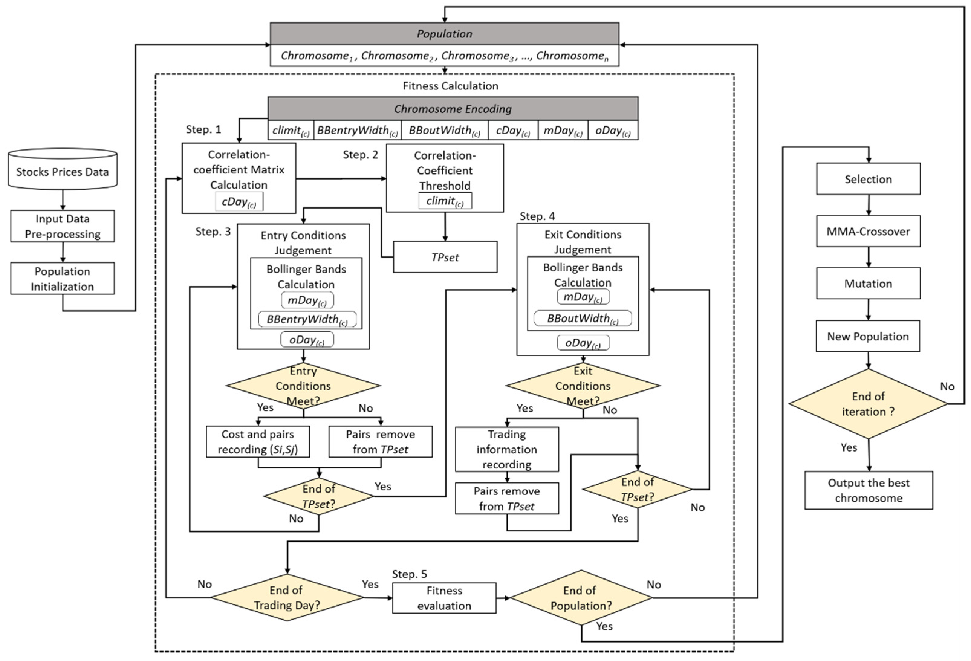
3.1. AGBCPT Flowchart
3.2. AGBCPT Components
3.2.1. Encoding Scheme
3.2.2. Initial Population
3.2.3. Fitness Function
3.2.4. Genetic Operations
3.3. Proposed AGBCPT
- Input:
- Selected companies: S = {s1, s2, …, si, …, sn}, 1 ≤ i ≤ n, where n is the number of companies, and the closing prices of all the companies, with the i-th represented as , 1 ≤ t ≤ dTotal, 1 ≤ i ≤ NumCompanies, where dTotal is the last trading day and NumCompanies is the number of companies.
- Parameters:
- Population size pSize, max generation maxGeneration, mutation rate mRate, crossover rate cRate, and parameter for the max-min arithmetical crossover operator d.
- Output:
- Chromosome with highest fitness value bestChro.
- STEP 1:
- Randomly initialize the population with population size pSize. Each chromosome has six genes: the correlation coefficient threshold (cLimit), the entry width of the Bollinger Bands (BBentryWidth), the out width of the Bollinger Bands (BBoutWidth), the correlation coefficient calculation days (cDay), the moving average calculation days (mDay), and the forward observation days (oDay).
- STEP 2:
- Use the following steps to calculate the correlation coefficient matrix of n companies MT(n).
- STEP 2.1:
- Obtain the historical closing prices CPsi and CPsj of two companies si and sj from the trading days (T − cDayq) to (T − 1) according to cDayq in chromosome Cq as
- Step 2.2:
- Calculate the correlation coefficient of si and sj using
- Step 2.3:
- Repeat Steps 2.1 and 2.2 to complete the correlation coefficient matrix MT(n).
- STEP 3:
- Use the following steps to select the stock pairs whose CCsisj is less than cLimitq and then calculate the stock pair’s entry and exit bands according to BBentryWidthq, BBoutWidthq, and mDayq of chromosome Cq.
- Step 3.1:
- Generate the trading pair candidate set according to TPset = {tp(si, sj)|CCsisj ≤ cLimitq}, where cLimitq is the correlation coefficient threshold from chromosome Cq.
- Step 3.2:
- Obtain the closing prices CPsi and CPsj from trading days (T − mDayq) to (T − 1) of both si and sj of tp(si, sj) in TPset as
- Step 3.3:
- Calculate the moving average values MAi(T) and MAj(T) of si and sj using the closing prices generated in the previous step as
- Step 3.4:
- Use the moving average value and BBentryWidthq to calculate the entry upper and lower bands of si and sj on day T based on Formulas (1) and (2) as
- Step 3.5:
- Use the moving average value and BBoutWidthq to calculate the exit upper and lower bands of si and sj on day T based on Formulas (3) and (4) as
- STEP 4:
- Use the following steps to determine whether to start pairs trading.
- Step 4.1:
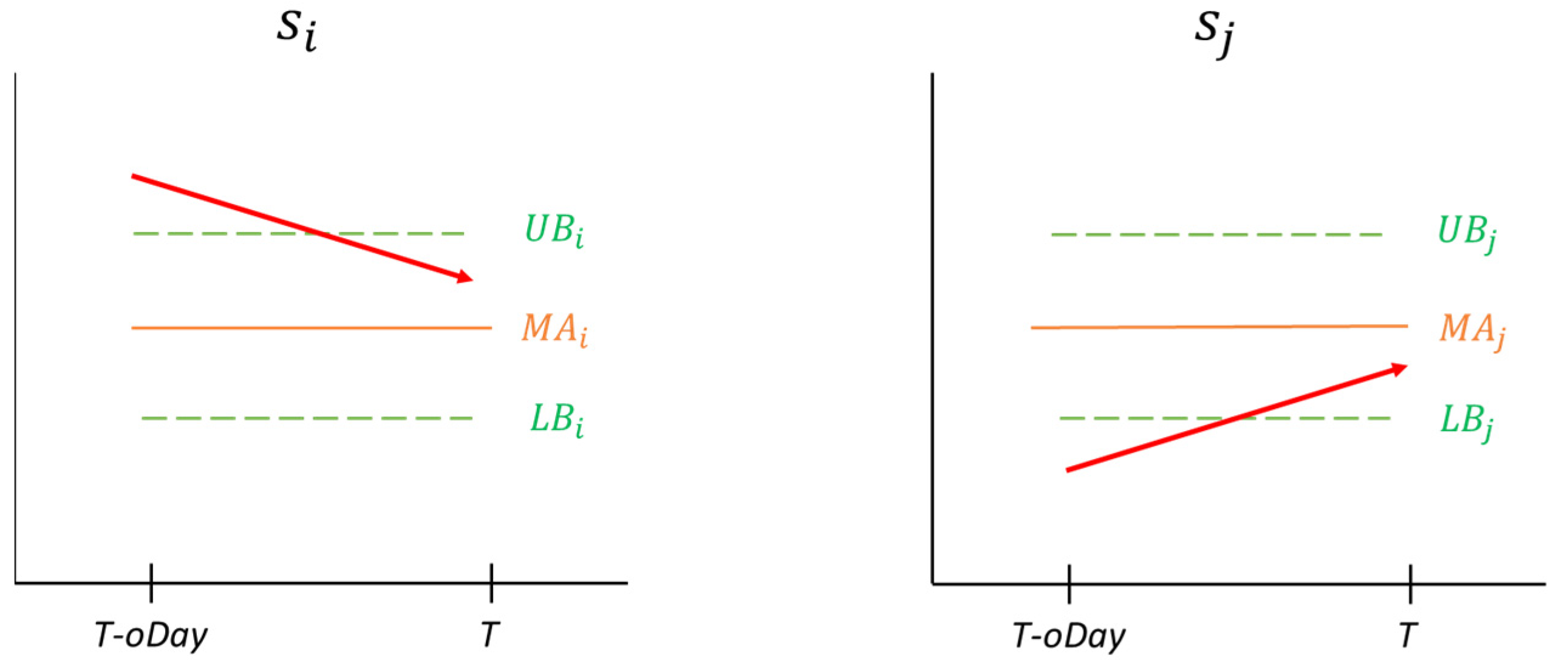
- Determine whether all trading pairs tp(si, sj) in TPset meet the following two entry conditions:Condition 1: The (T − oDayq) closing price of the stock si crosses the upper band of buy (UB) downward on T day:Condition 2: The (T − oDayq) closing price of the stock sj crosses the lower band of buy (LB) upward on T day:when the two entry conditions are met, as shown in Figure 2, it is expected that si will continue to fall, and sj will continue to rise. Hence, short si and long sj.
- Step 4.2:
- Short one unit of stock si and buy an integer number of stock sj at the same cost to stock si when > ; otherwise, buy one unit of stock si and short an integer number of stock sj at the same cost as stock sj.
- Step 4.3:
- Record the cost tpC(si, sj) of this trading pair tp(si, sj).
- Step 4.4:
- Remove tp(si, sj) from TPset if the entry conditions are not met.
- Step 4.5:
- Go to Step 4.1 to determine the entry conditions of the next pair in TPset.
- STEP 5:
- Use the following steps to determine whether to finish every trading pair in TPset.
- Step 5.1:
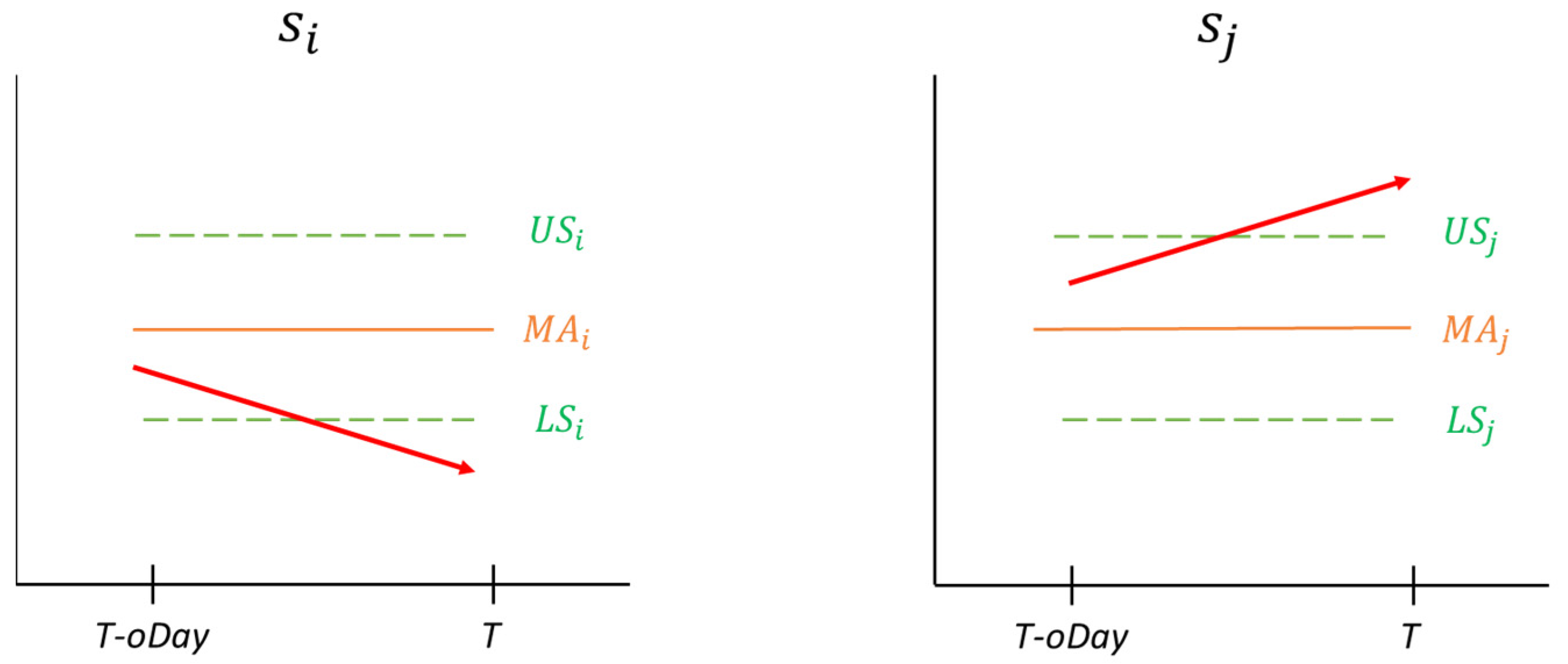
- Determine whether all trading pairs tp(si, sj) in TPset meet the following exit conditions:Condition 3: The (T − oDayq) closing price of the stock si crosses the lower band of sell (LS) downward on the closing price at day T:Condition 4: The (T − oDayq) closing price of the stock sj crosses the upper band of sell (US) upward on the closing price at day T:when the above exit conditions are satisfied, as shown in Figure 3, the transaction is closed. If it enters the market by shorting si and longing sj, then it closes tp(si, sj) by longing si and shorting sj. Likewise, if it enters the market by longing si and shorting sj, then it closes the trading pair by shorting si and longing sj.
- Step 5.2:
- Record the income tpP(Si, Sj) of tp(si, sj).
- Step 5.3:
- Record the profit Profith(Si, Sj) of tp(si, sj).
- Step 5.4:
- Remove tp(si, sj) from TPset.
- Step 5.5:
- Record the transaction frequency of the trading pair as totalSell = totalSell + 1.
- Step 5.6:
- Go to Step 5.1 to determine the exit conditions of the next trading pair in TPset.
- STEP 6:
- If the stop conditions are not met (T + 1 < dTotal), set T = T + 1 and go to Step 2 to continue the entry and exit judgment. Otherwise, go to Step 7.
- STEP 7:
- Evaluate the fitness value of a chromosome by the average return and the risk of all trading pairs, as mentioned in the previous section.
- STEP 8:
- Repeat Steps 2 to 7 until the fitness value of every chromosome in the population is calculated.
- STEP 9:
- If the stop condition Generation = maxGeneration is met, then terminate the evolution process and goes to Step 14. Otherwise, set Generation = Generation + 1 and go to Step 10.
- STEP 10:
- Execute tournament selection to generate the next population.
- Step 10.1:
- Select two chromosomes randomly from the population and compare their fitness values. The chromosome with the higher fitness value is kept for the next population.
- Step 10.2:
- Repeat Step 10.1 until pSize chromosomes have been generated.
- STEP 11:
- Execute MMA crossover operator with parameter d and crossover rate cRate.
- STEP 12:
- Execute mutation operator to generate a new offspring with mutation rate mRate.
- STEP 13:
- Go to Step 2 to evaluate the fitness of new chromosomes.
- STEP 14:
- Output the chromosome with the highest fitness value as the best chromosome bestChro.
3.4. AGBCPT Example
- STEP 1:
- The population is initialized. Since pSize is 5, the initial population can be randomly generated according to the encoding schema and the predefined ranges of parameters. Take C1 as an example. The six parameters are generated as [−0.98, 1.0, 0.5, 10, 10, 1]. In the same way, the initial population is formed and shown in Table 5.
- STEP 2:
- For every chromosome, the correlation coefficient matrix MT(n) of the six companies is calculated by gene cDayq of chromosome Cq.
- Step 2.1:
- Take C1 as an example. Because the value of cDay1 is 10, T starts from 11. The historical closing prices of S1101 and S1102 from trading days (T − 10) to (T − 1) are shown asCPS1101 = {10.5, 11, 11.25, 11.5, 12, 12.25, 13, 13.5, 13.75, 14.25}, andCPS1102 = {21, 22, 23, 24, 25, 26, 27, 28, 29, 30}.
- Step 2.2:
- The correlation coefficient of the two companies CCS1101,S1102 is then calculated as 0.9941.
- Step 2.3:
- Steps 2.1 and 2.2 are repeated to generate the correlation coefficient of any two companies. The resultant matrix MT(n) is shown in Table 6.
- STEP 3:
- The cLimitq value is used to find the qualified stock pairs and BBentryWidthq, BBoutWidthq, and mDayq are used to generate the entry and exit bands.
- Step 3.1:
- Take C1 as an example. Because cLimitq is −0.98 and the CCS1102,S2412 and CCS1102,S2474 are −0.9861 and −0.9819, meeting the condition, they are inserted into the trading pair candidate set TPset = {tp(S1102, S2412), tp(S1102, S2474)}.
- Step 3.2:
- Since mDay1 of C1 is 10, the stock price series from Day 1 (=11 − 10) to 10 (=11 − 1) of companies S1102 and S2412 of tp(S1102, S2412) in TPset are generated asS1102: {21, 22, 23, 24, 25, 26, 27, 28, 29, 30}, andS2412: {71.5, 68, 66.5, 65, 63, 60, 57, 58, 56, 54}.
- Step 3.3:
- Using the 10-day moving average of S1102 and S2412 as examples, the values of MA1102(11) and MA2412(11) are calculated as 25.5 and 61.9.
- Step 3.4:
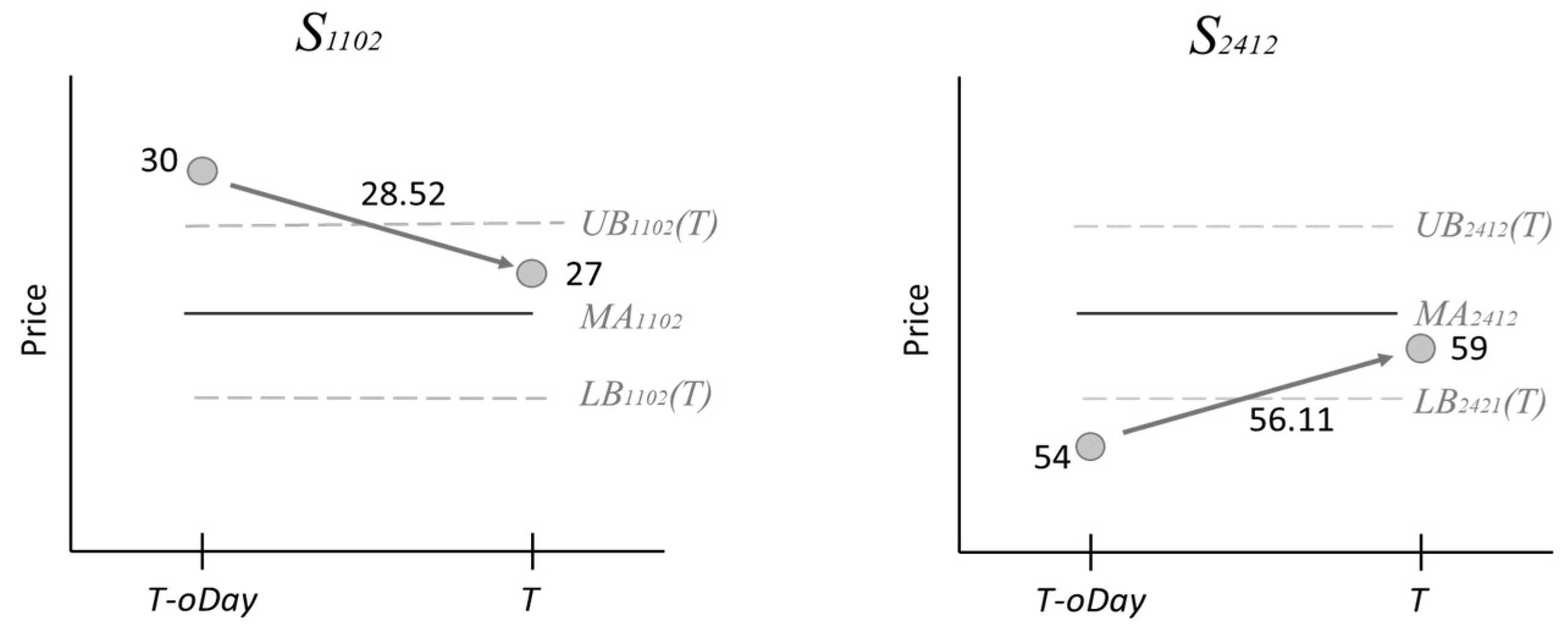
- The moving average value and BBentryWidth1 are used to calculate the entry upper and lower bands of S1102 and S2412 asUB1102(11) = 25.5 + 1 × 3.02 = 28.52,LB1102(11) = 25.5 − 1 × 3.02 = 22.47,UB2412(11) = 61.9 + 1 × 5.78 = 67.68, andLB2412(11) = 61.9 − 1 × 5.78 = 56.11.
- Step 3.5:
- The moving average value and BBoutWidth1 are used to calculate the exit upper and lower bands of S1102 and S2412 asUS1102(11) = 25.5 + 0.5 × 3.02 = 27.01,US2412(11) = 61.9 + 0.5 × 5.78 = 64.79,LS1102(11) = 25.5 − 0.5 × 3.02 = 23.99, andLS2412(11) = 61.9 − 0.5 × 5.78 = 59.01.
- STEP 4:
- The oDayq, entry upper and lower bands are used to determine whether trading pair tp(si, sj) in TPset meet the conditions to enter the market.
- Step 4.1:
- Take trading pair tp(S1102, S2412) as an example. It is checked to determine whether it meets the following entry conditions at trading Day T (=11). Since oDay1 of C1 is 1, according to the stock prices on Day 10 (=11 − 1) of S1102 and S2412, the two conditions are shown as
- Step 4.2:
- Because the closing price on trading Day 11 of (59) is greater than (27), their ratio is rounded to 2. Hence, the trading strategy then longs one unit of S2412 and shorts two units of S1102. Thus, their investment capital is nearly equal.
- Step 4.3:
- The cost of this trading pair tpC(1102, 2412) is then recorded. The cost of longing S2412 is 59,084 (=59 × 1000 × 1 × (1 + 0.001425)), the cost of shorting S1102 is 54,239 (=27 × 1000 × 2 × (1 + 0.004425)), and tpC(S1102, S2412) is 113,323 (=59,084 + 54,239).
- Step 4.4:
- If the entry condition of tp(si, sj) is not met, then it is removed from TPset.
- Step 4.5:
- Steps 4.1 to 4.4 are repeated to determine the entry condition of every pair tp(si, sj) in TPset until all pairs have been checked.
- STEP 5:
- The upper and lower exit bands are then used to determine whether tp(S1102, S2412) has met the conditions to exit the market.
- Step 5.1:
- Take trading pair tp(S1102, S2412) as an example. It is checked to determine whether it meets the following exit conditions on trading Day 12. Since oDay1 of C1 is 1, according to the stock prices on Day 11 (=12 − 1) of both S1102 and S2412 of tp(S1102, S2412), the two conditions arewhen the above exit conditions are met, the trading strategy then longs S1102 and shorts S2412, as shown in Step 5.2: Longing stock S1102 and shorting S2412 yields 48,068 (=24 × 1000 × 2 × (1 + 0.001425)) and 68,301 (=68 × 1000 × 1 × (1 + 0.004425)). The trading result of trading pair tpP(S1102, S2412), which is 15,388 (=(54,239 – 48,068) + (68,301 – 59,084)), is then recorded.
- Step 5.3:
- The profit of the trading pair, profit(1102,2412), is then recorded as
- Step 5.4:
- Pair tp(S1102, S2412) is removed from TPset.
- Step 5.5:
- The number of transactions is set to totalSell = totalSell + 1.
- Step 5.6:
- Steps 5.1 to 5.5 are repeated to determine the exit condition of the next pair tp(si, sj) in TPset until all the pairs have been checked.
- STEP 6:
- The trading stop conditions are checked. If stop condition (T + 1 < dTotal) is not met, then T is set to T + 1, Step 2 is executed, and the entry and exit judgment is continued for the next trading day. Otherwise, Step 7 is executed.
- STEP 7:
- Because the three profits of the trading pair are calculated as 13.57%, 10.15%, and 1%, the risk of the trading pair is 1%, which is the minimum value of the three profits. The fitness value of C1 is then calculated by the total profit and risk of the trading pair as 24.72 (=24.72%/1%).
- STEP 8:
- Steps 2 to 7 are repeated to calculate the fitness values of all chromosomes, yielding the results shown in Table 7.
- STEP 9:
- If the stop condition is met, Step 14. Otherwise, Step 10 is executed to generate next population.
- STEP 10:
- Tournament selection is used to generate the next population.
- Step 10.1:
- Take the two chromosomes shown in Table 8 as an example. Because the fitness value of C1 is greater than C4, C1 is retained for the next population.
- Step 10.2:
- Step 10.1 is repeated until the number of chromosomes is equal to 5.
- STEP 11:
- The MMA crossover operator is applied to generate offspring. The MMA parameter d and the crossover rate cRate are set to 0.7 and 0.8. For every two chromosomes, four new chromosomes are generated as candidate offspring. Take chromosomes C1 and C2 as an example. After crossover, the final offspring are shown in Table 9.
- STEP 12:
- The one-point mutation operator is executed to generate new offspring according to the mutation rate.
- STEP 13:
- After executing the crossover and mutation operators, Steps 2 to 8 are used to calculate the fitness value of the new chromosomes.
- STEP 14:
- The chromosome with the highest fitness value is outputted. In this example, according to Table 7, C1: [−0.98, 1.0, 0.5, 10, 10, 1] is selected and outputted as the parameters for trading.
4. Experimental Results and Discussion
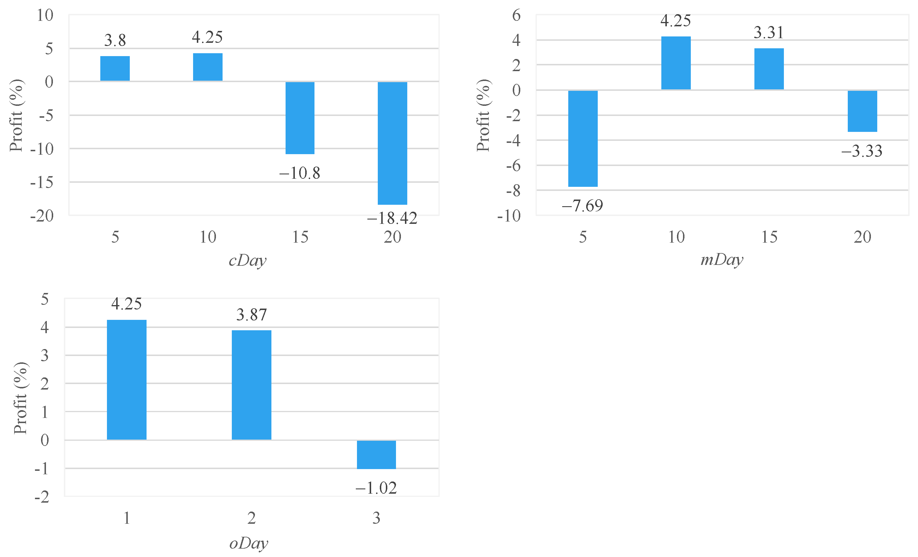
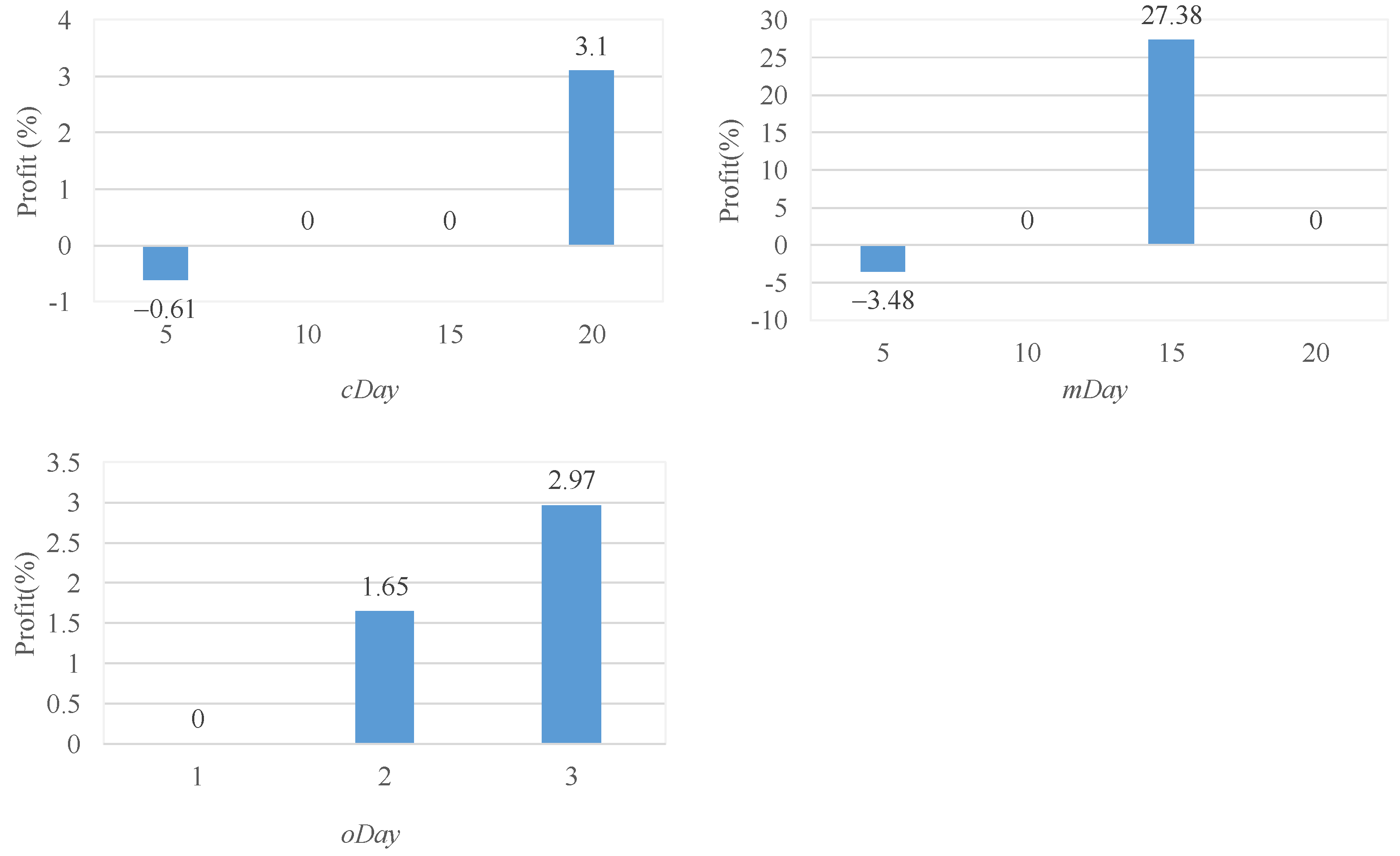
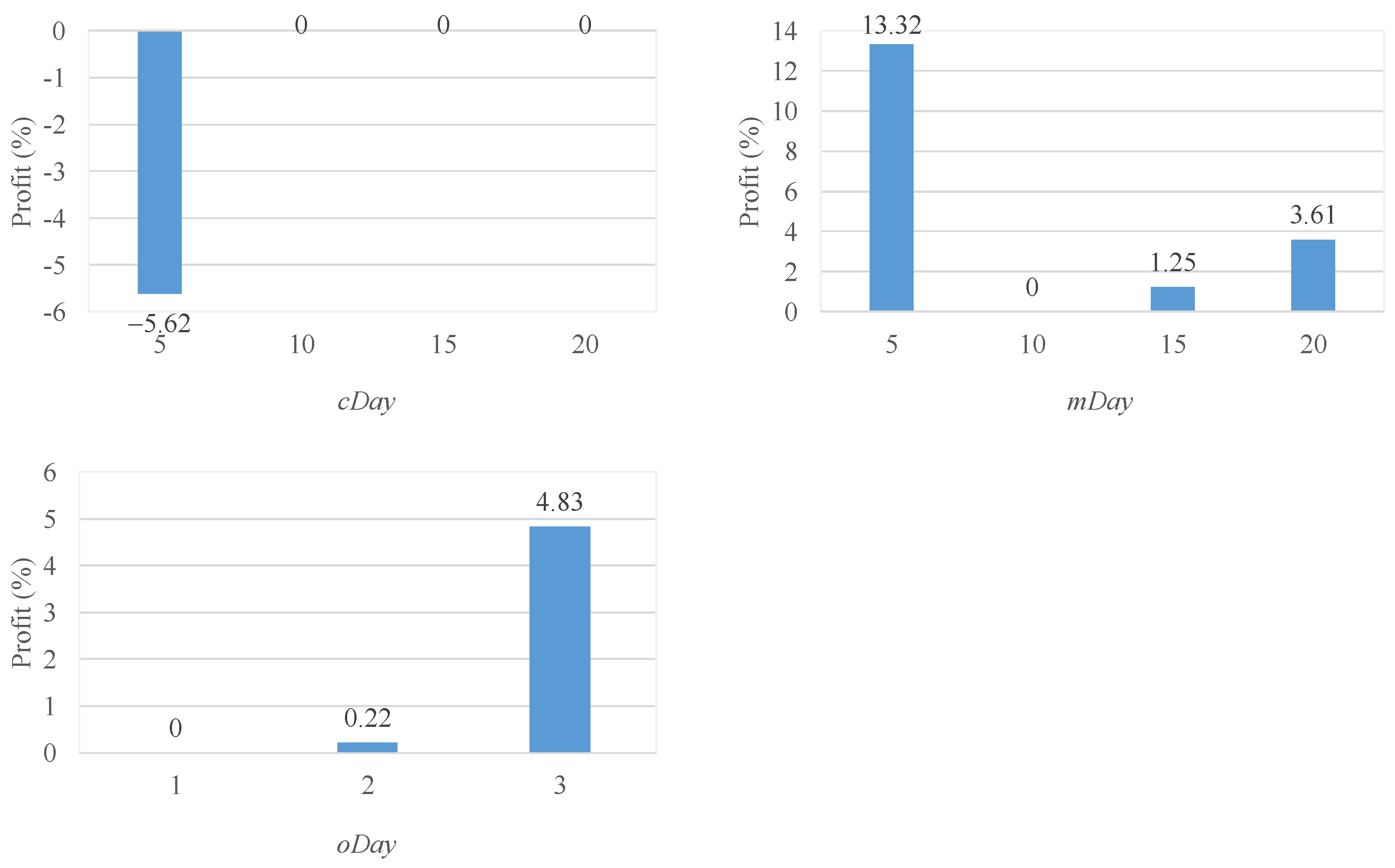
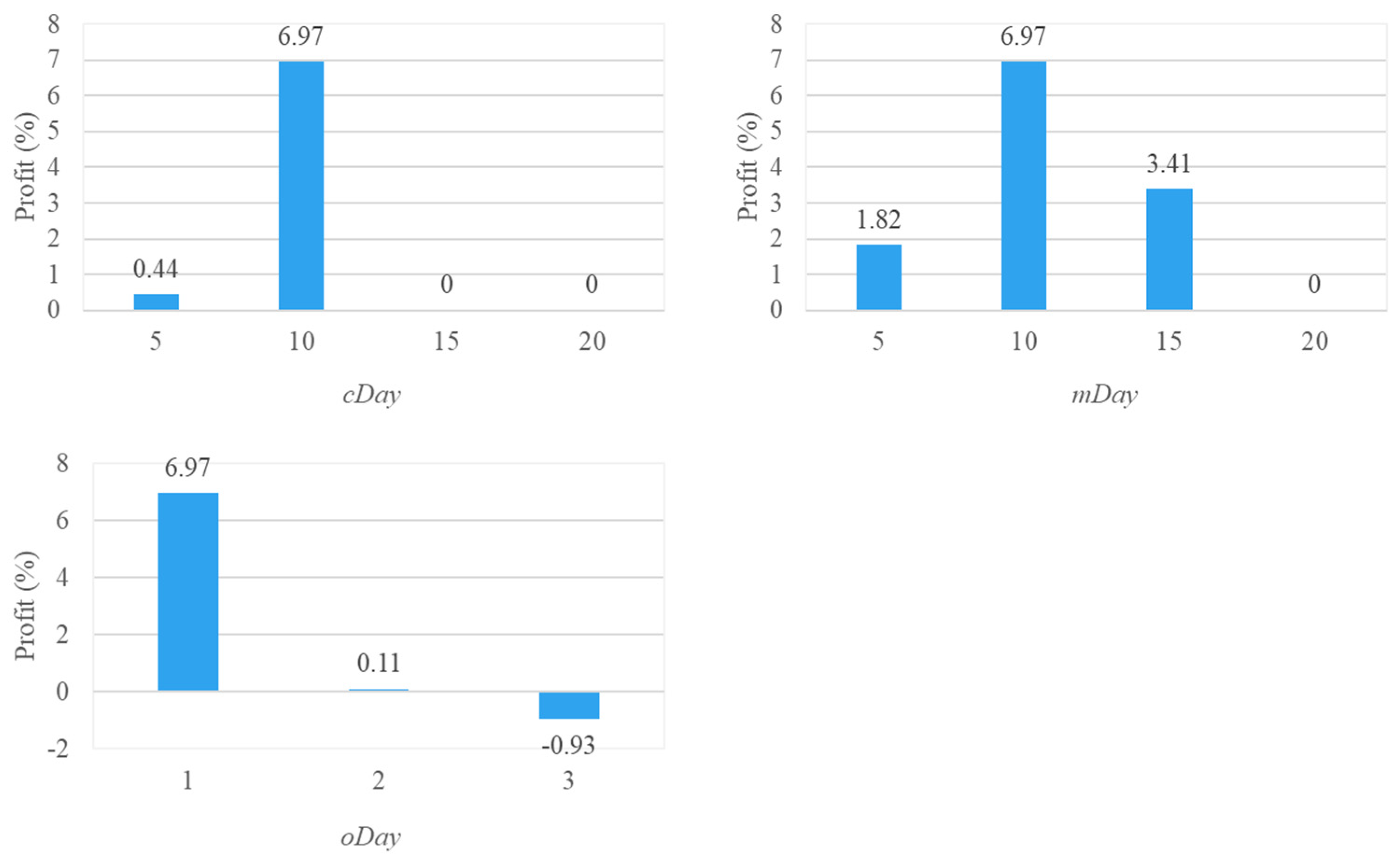
4.1. Impact of Three New Parameters on Pairs Trading Strategy
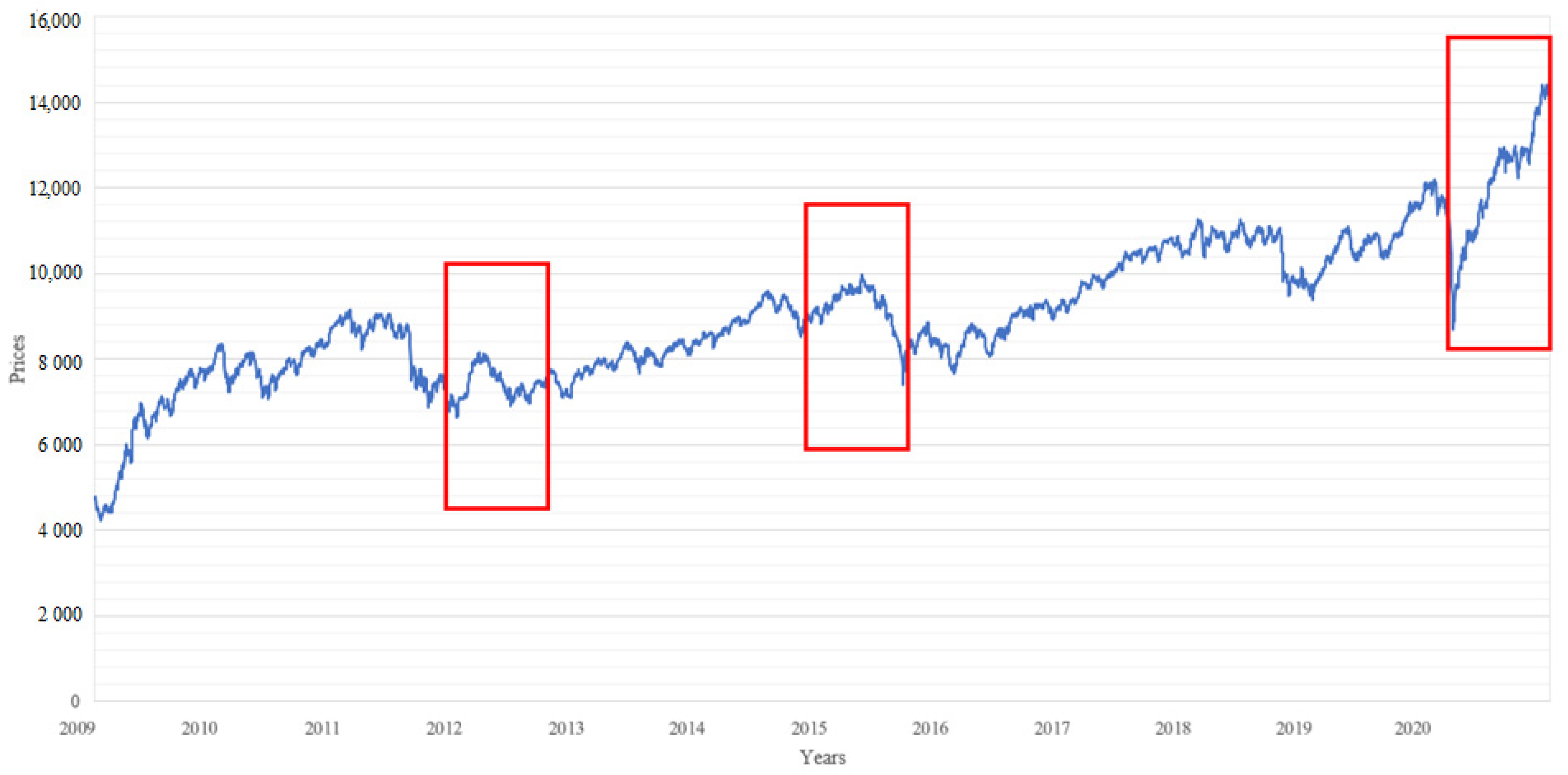
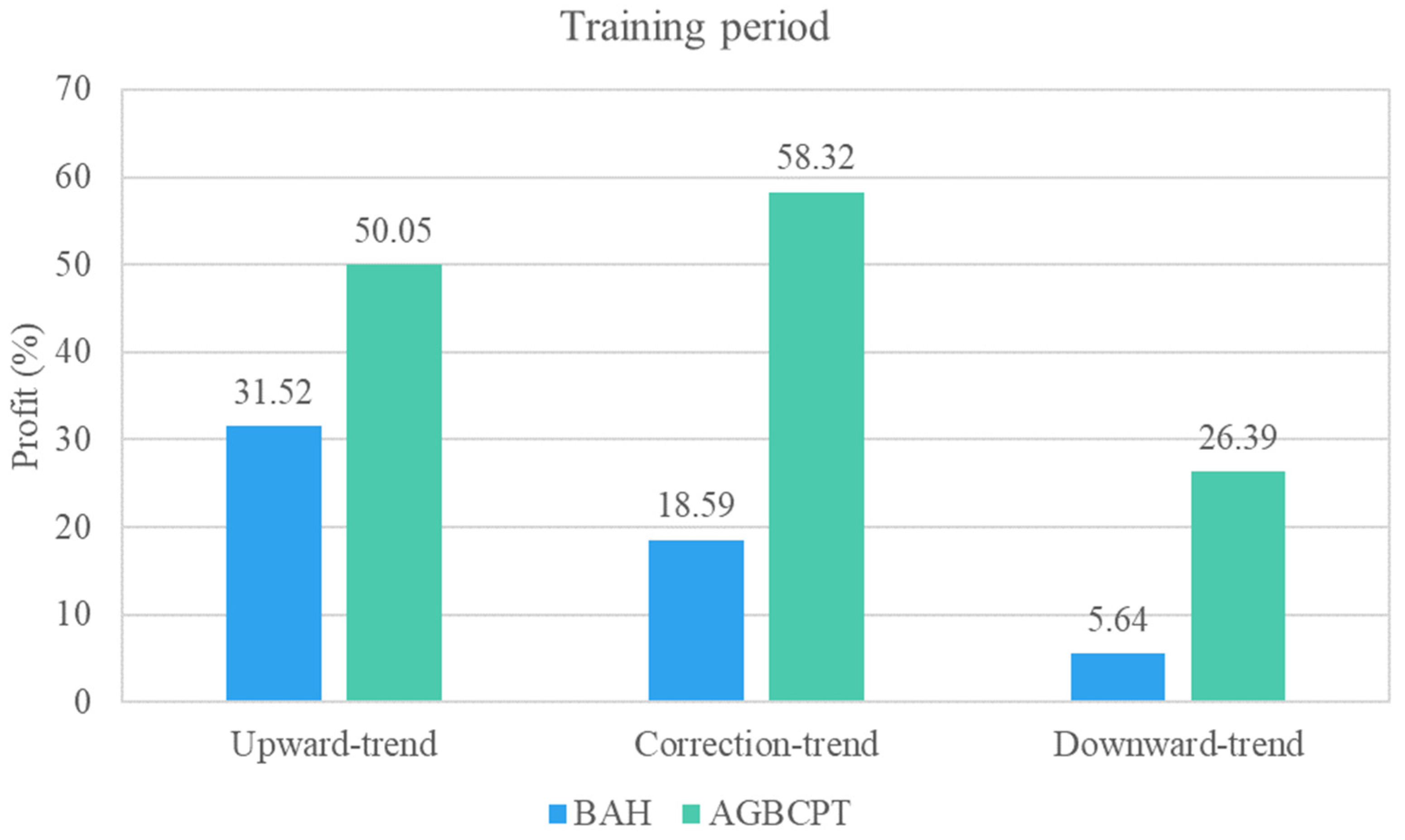
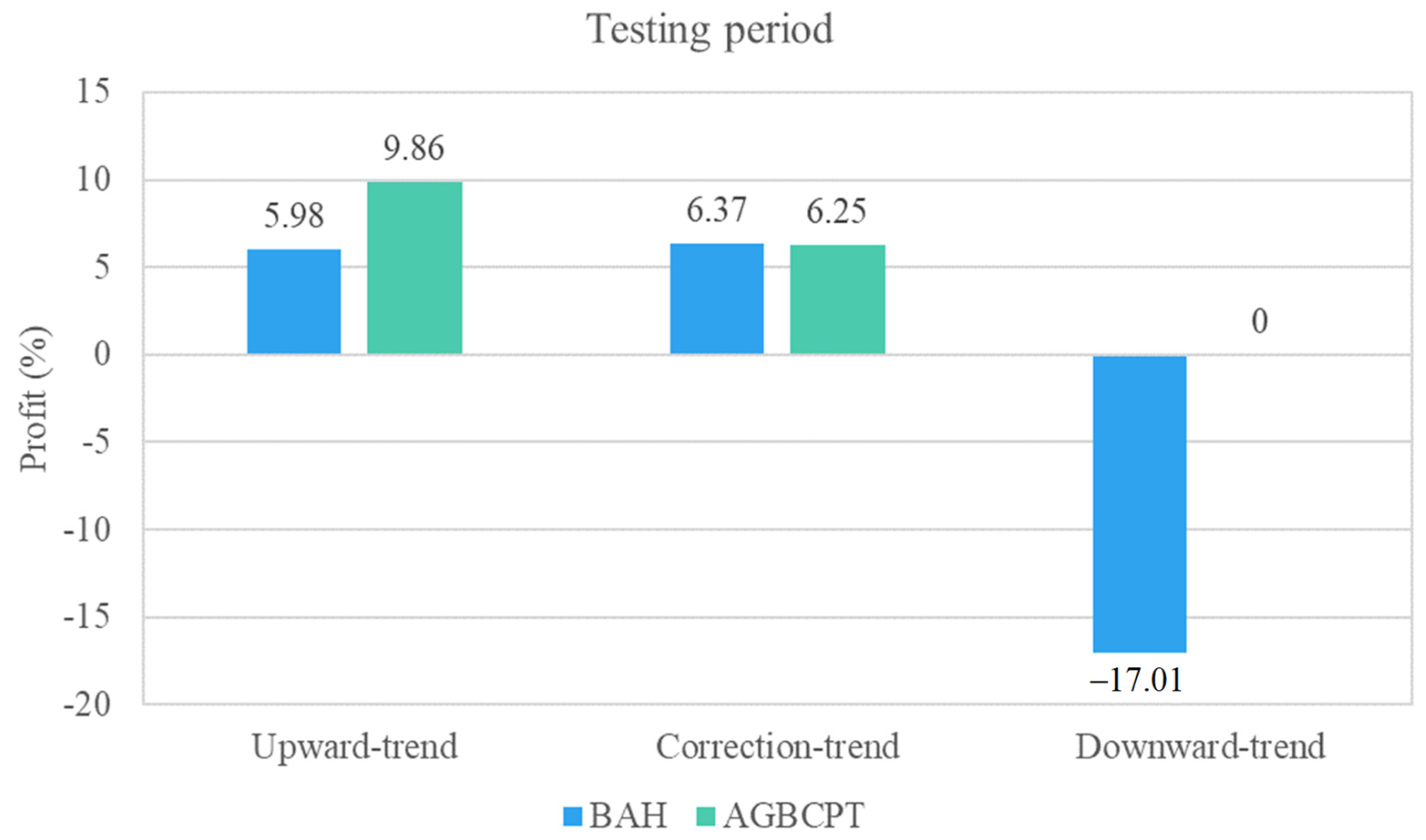
4.2. Impact of AGBCPT under Different Stock Trends
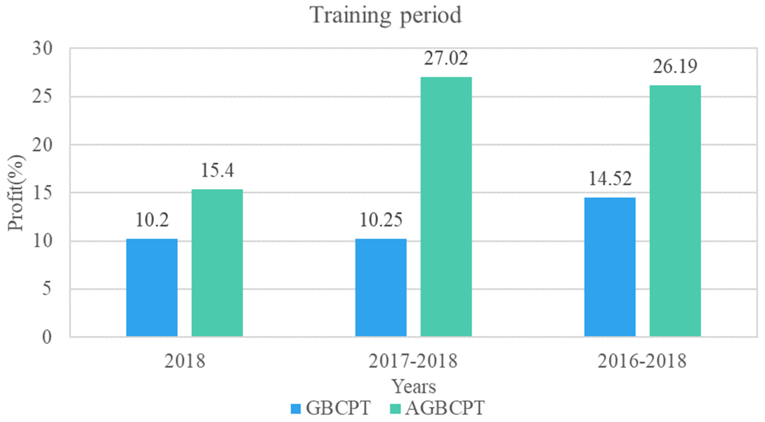
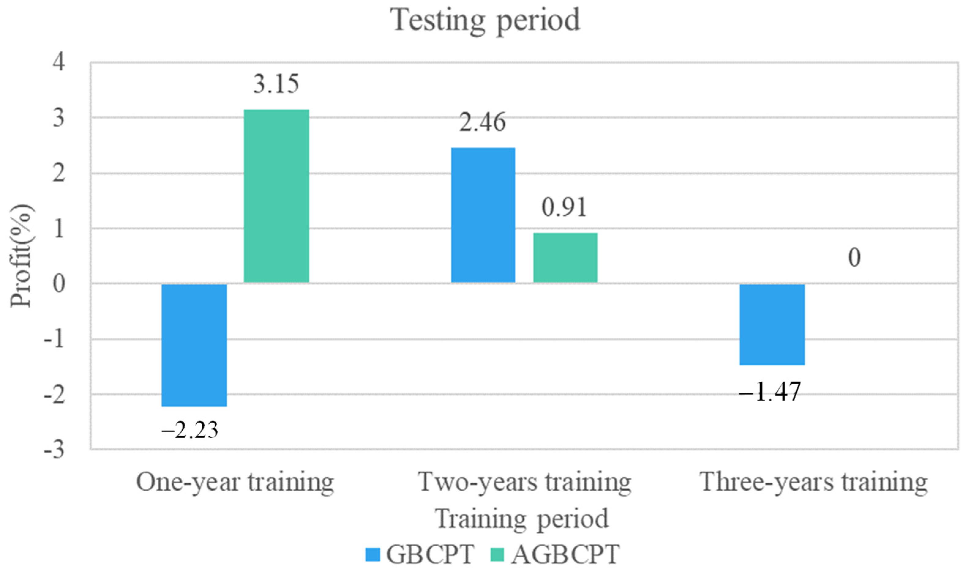
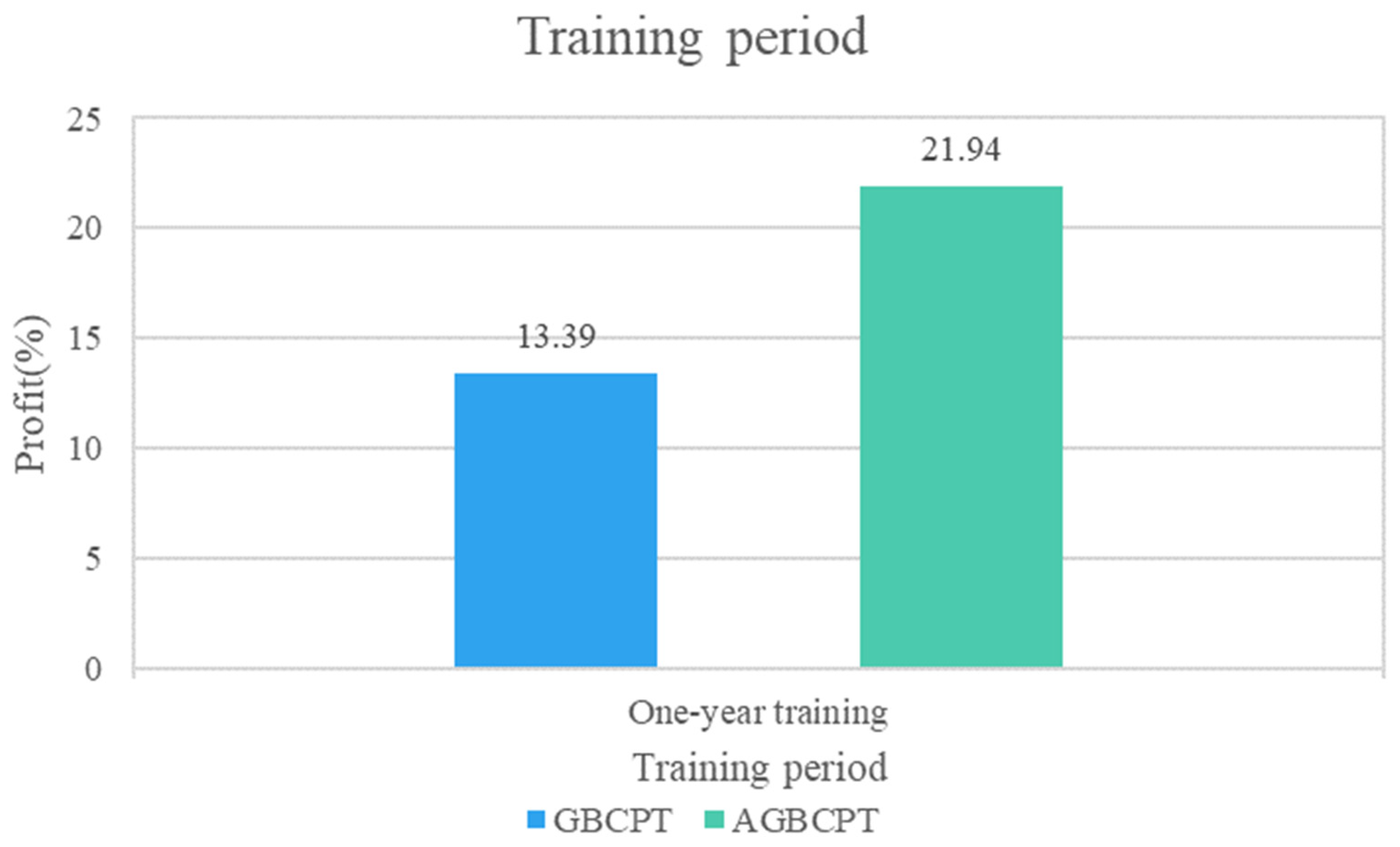
4.3. Comparison of AGBCPT and GBCPT
4.4. Discussion
5. Conclusions and Future Work
Author Contributions
Funding
Institutional Review Board Statement
Informed Consent Statement
Data Availability Statement
Conflicts of Interest
References
- Chang, H.-H.; Dai, T.-S.; Wang, K.-L.; Chu, C.-H.; Wang, J.-Z. Improving pair trading performances with structural change detections and revised trading strategies. In Proceedings of the 2020 International Conference on Pervasive Artificial Intelligence (ICPAI), Taipei, Taiwan, 3–5 December 2020; pp. 105–109. [Google Scholar]
- Ding, W.; Mazouz, K.; Wang, Q. Volatility timing, sentiment, and the short-term profitability of VIX-based cross-sectional trading strategies. J. Empir. Financ. 2021, 63, 42–56. [Google Scholar] [CrossRef]
- Prasetijo, A.; Saputro, T.A.; Windasari, I.P.; Windarto, Y.E. Buy/sell signal detection in stock trading with Bollinger Bands and parabolic SAR: With web application for proofing trading strategy. In Proceedings of the 2017 4th International Conference on Information Technology, Computer, and Electrical Engineering (ICITACEE), Semarang, Indonesia, 18–19 October 2017; pp. 41–44. [Google Scholar]
- Wu, X.; Chen, H.; Wang, J.; Troiano, L.; Loia, V.; Fujita, H. Adaptive stock trading strategies with deep reinforcement learning methods. Inf. Sci. 2020, 538, 142–158. [Google Scholar]
- Wu, M.-E.; Syu, J.-H.; Lin, J.C.-W.; Ho, J.-M. Effective fuzzy system for qualifying the characteristics of stocks by random trading. IEEE Trans. Fuzzy Syst. 2022. [Google Scholar] [CrossRef]
- Wu, J.M.-T.; Sun, L.; Srivastava, G.; Lin, J.C.-W. A long short-term memory network stock price prediction with leading indicators. Big Data 2021, 9, 343–357. [Google Scholar] [PubMed]
- Zhang, W.; Wang, L.; Xie, L.; Feng, K.; Liu, X. TradeBot: Bandit learning for hyper-parameters optimization of high frequency trading strategy. Pattern Recognit. 2021, 124, 108490. [Google Scholar] [CrossRef]
- Cocco, L.; Tonelli, R.; Marchesi, M. An agent-based artificial market model for studying the bitcoin trading. IEEE Access 2019, 7, 42908–42920. [Google Scholar] [CrossRef]
- Ferreira, F.G.D.C.; Gandomi, A.H.; Cardoso, R.T.N. Artificial intelligence applied to stock market trading: A review. IEEE Access 2021, 9, 30898–30917. [Google Scholar]
- Jirapongpan, R.; Phumchusri, N. Prediction of the Profitability of Pairs Trading Strategy Using Machine Learning. In Proceedings of the 2020 IEEE 7th International Conference on Industrial Engineering and Applications (ICIEA), Bangkok, Thailand, 16–21 April 2020; pp. 1025–1030. [Google Scholar]
- Mochón, A.; Quintana, D.; Sáez, Y.; Isasi, P.; Mochón, M.A. Soft computing techniques applied to finance. Appl. Intell. 2007, 29, 111–115. [Google Scholar] [CrossRef] [Green Version]
- Stadnik, B. Interest rates sensitivity arbitrage—Theory and practical assessment for financial market trading. J. Bus. Manag. Econ. Eng. 2021, 19, 12–23. [Google Scholar] [CrossRef]
- Chen, S.; Zhou, C. Stock prediction based on genetic algorithm feature selection and long short-term memory neural network. IEEE Access 2021, 9, 9066–9072. [Google Scholar] [CrossRef]
- Kim, K.-J.; Han, I. Genetic algorithms approach to feature discretization in artificial neural networks for the prediction of stock price index. Expert Syst. Appl. 2000, 19, 125–132. [Google Scholar] [CrossRef]
- Patel, J.; Shah, S.; Thakkar, P.; Kotecha, K. Predicting stock market index using fusion of machine learning techniques. Expert Syst. Appl. 2015, 42, 2162–2172. [Google Scholar] [CrossRef]
- Shen, J.; Shafiq, M.O. Short-term stock market price trend prediction using a comprehensive deep learning system. J. Big Data 2020, 7, 66. [Google Scholar] [CrossRef]
- Chen, C.-H.; Chen, Y.-H.; Diaz, V.G.; Lin, J.C.-W. An intelligent trading mechanism based on the group trading strategy portfolio to reduce massive loss by the grouping genetic algorithm. Electron. Commer. Res. 2021. [Google Scholar] [CrossRef]
- Chen, C.-H.; Lu, C.-Y.; Hong, T.-P.; Lin, J.C.-W.; Gaeta, M. An effective approach for the diverse group stock portfolio optimization using grouping genetic algorithm. IEEE Access 2019, 7, 155871–155884. [Google Scholar] [CrossRef]
- Lim, S.; Kim, M.-J.; Ahn, C.W. A genetic algorithm (GA) approach to the portfolio design based on market movements and asset valuations. IEEE Access 2020, 8, 140234–140249. [Google Scholar] [CrossRef]
- Bowen, D.A.; Hutchinson, M.C. Pairs trading in the UK equity market: Risk and return. Eur. J. Financ. 2016, 22, 1363–1387. [Google Scholar] [CrossRef]
- Elliott, R.J.; Hoek, J.V.D.; Malcolm, W.P. Pairs trading. Quant. Financ. 2005, 5, 271–276. [Google Scholar] [CrossRef]
- Flori, A.; Regoli, D. Revealing pairs-trading opportunities with long short-term memory networks. Eur. J. Oper. Res. 2021, 295, 772–791. [Google Scholar] [CrossRef]
- Krauss, C. Statistical arbitrage pairs trading strategies: Review and outlook. J. Econ. Surv. 2016, 31, 513–545. [Google Scholar] [CrossRef]
- Sarmento, S.M.; Horta, N. Enhancing a pairs trading strategy with the application of machine learning. Expert Syst. Appl. 2020, 158, 113490. [Google Scholar] [CrossRef]
- Gatev, E.G.; Goetzmann, W.N.; Rouwenhorst, K.G. Pairs trading: Performance of a relative-value arbitrage rule. Rev. Financ. Stud. 2006, 19, 797–827. [Google Scholar] [CrossRef] [Green Version]
- Fil, M.; Kristoufek, L. Pairs trading in cryptocurrency markets. IEEE Access 2020, 8, 172644–172651. [Google Scholar] [CrossRef]
- Oh, E.; Son, S.-Y. Pair matching strategies for prosumer market under guaranteed minimum trading. IEEE Access 2018, 6, 40325–40333. [Google Scholar] [CrossRef]
- Huang, C.C. Correlation-Based Pair Trading Optimization Techniques. Master’s Thesis, Department of Computer Science and Information Engineering, Tamkang University, Taipei, Taiwan, 2020. [Google Scholar]
- Shen, L.; Shen, K.; Yi, C.; Chen, Y. An evaluation of pairs trading in commodity futures markets. In Proceedings of the 2020 IEEE International Conference on Big Data (Big Data), Atlanta, GA, USA, 10–13 December 2020; pp. 5457–5462. [Google Scholar]
- Clegg, M.; Krauss, C. Pairs trading with partial cointegration. Quant. Financ. 2018, 18, 121–138. [Google Scholar] [CrossRef] [Green Version]
- Do, B.; Faff, R. Does simple pairs trading still work? Financ. Anal. J. 2010, 66, 83–95. [Google Scholar] [CrossRef]
- Do, B.; Faff, R. Are pairs trading profits robust to trading costs? J. Financ. Res. 2012, 35, 261–287. [Google Scholar] [CrossRef]
- Liang, S.; Lu, S.; Lin, J.; Wang, Z. Low-latency hardware accelerator for improved engle-granger cointegration in pairs trading. IEEE Trans. Circuits Syst. I Regul. Pap. 2021, 68, 2911–2924. [Google Scholar] [CrossRef]
- Liu, B.; Chang, L.-B.; Geman, H. Intraday pairs trading strategies on high frequency data: The case of oil companies. Quant. Financ. 2017, 17, 87–100. [Google Scholar] [CrossRef] [Green Version]
- Rad, H.; Low, R.K.Y.; Faff, R. The profitability of pairs trading strategies: Distance, cointegration and copula methods. Quant. Financ. 2016, 16, 1541–1558. [Google Scholar] [CrossRef]
- Ramos-Requena, J.; Trinidad-Segovia, J.; Sánchez-Granero, M. Introducing Hurst exponent in pair trading. Phys. A Stat. Mech. Its Appl. 2017, 488, 39–45. [Google Scholar] [CrossRef]
- Jacobs, H.; Weber, M. On the determinants of pairs trading profitability. J. Financ. Mark. 2015, 23, 75–97. [Google Scholar] [CrossRef]
- Rende, J. Pairs trading with the persistence-based decomposition model. Manag. Econ. 2020, 20, 151. [Google Scholar] [CrossRef]
- Stäbinger, J.; Endres, S. Pairs trading with a mean-reverting jump-diffusion model on high-frequency data. Quant. Financ. 2018, 18, 1735–1751. [Google Scholar] [CrossRef] [Green Version]
- Fallahpour, S.; Hakimian, H.; Taheri, K.; Ramezanifar, E. Pairs trading strategy optimization using the reinforcement learning method: A cointegration approach. Soft Comput. 2016, 20, 5051–5066. [Google Scholar] [CrossRef]
- Lintilhac, P.S.; Tourin, A. Model-based pairs trading in the bitcoin markets. Quant. Financ. 2016, 17, 703–716. [Google Scholar] [CrossRef]
- Katoch, S.; Chauhan, S.S.; Kumar, V. A review on genetic algorithm: Past, present, and future. Multimed. Tools Appl. 2021, 80, 8091–8126. [Google Scholar] [CrossRef]
- Whitley, D. A genetic algorithm tutorial. Stat. Comput. 1994, 4, 65–85. [Google Scholar] [CrossRef]
- Chen, Y.J.; Lin, J.A.; Chen, Y.M.; Wu, J.H. Financial forecasting with multivariate adaptive regression splines and queen genetic algorithm-support vector regression. IEEE Access 2019, 7, 112931–112938. [Google Scholar] [CrossRef]
- Huang, C.-F. A hybrid stock selection model using genetic algorithms and support vector regression. Appl. Soft Comput. 2012, 12, 807–818. [Google Scholar] [CrossRef]
- Cheong, M.-S.; Wu, M.-C.; Huang, S.-H. Interpretable stock anomaly detection based on spatio-temporal relation networks with genetic algorithm. IEEE Access 2021, 9, 68302–68319. [Google Scholar] [CrossRef]
- Sermpinis, G.; Stasinakis, C.; Zong, X. Deep Reinforcement Learning and Genetic Algorithm for a Pairs Trading Task on Commodities. 2020. Available online: https://ssrn.com/abstract=3770061 (accessed on 16 January 2022). [CrossRef]
- Goldkamp, J.; Dehghanimohammadabadi, M. Evolutionary multi-objective optimization for multivariate pairs trading. Expert Syst. Appl. 2019, 135, 113–128. [Google Scholar] [CrossRef]
- Huang, C.-F.; Hsu, C.-J.; Chen, C.-C.; Chang, B.R.; Li, C.-A. An intelligent model for pairs trading using genetic algorithms. Comput. Intell. Neurosci. 2015, 2015, 939606. [Google Scholar] [CrossRef] [PubMed] [Green Version]
- Windasari, I.P.; Prasetijo, A.; Pangabean, R.P. Indonesia stock exchange securities buy/sell signal detection using Bollinger Bands and Williams percent range. In Proceedings of the 2018 International Seminar on Research of Information Technology and Intelligent Systems (ISRITI), Yogyakarta, Indonesia, 21–22 November 2018; pp. 633–636. [Google Scholar]


| Chromosome Cq | |||||
|---|---|---|---|---|---|
| cLimitq | BBentryWidthq | BBoutWidthq | mDayq | cDayq | oDayq |
| Name | Abbreviation | Range |
|---|---|---|
| Correlation coefficient threshold | cLimit | −1 < climit < 1 |
| Entry width of Bollinger Bands | BBentryWidth | 0 < BBentryWidth < 2 |
| Out width of Bollinger Bands | BBoutWidth | 0 < BBoutWidth < BBentryWidth |
| Moving average calculation days | mDay | 5 ≤ mDay ≤ 20 |
| Correlation coefficient calculation days | cDay | 5 ≤ cDay ≤ 20 |
| Forward observation days | oDay | 1 ≤ oDay ≤ 3 |
| Notation | Description |
|---|---|
| cLimit | Correlation coefficient threshold |
| dTotal | Final trading day |
| mDay | Moving average calculation days |
| cDay | Correlation coefficient calculation days |
| oDay | Forward observation days |
| T | Trading day |
| BBentryWidth | Entry width of Bollinger Bands |
| BBoutWidth | Out width of Bollinger Bands |
| TPset = Ø | Trading pair candidate set |
| tp(si, sj) = (si, sj) | Trading pair set (si, sj) |
| tpC(si, sj) | Trading pair cost (si, sj) |
| tpP(si, sj) | Trading pair income (si, sj) |
| Profit(si, sj) | Trading pair profit (si, sj) |
| Stock ID | Stock Price Series |
|---|---|
| S1101 | 10.5, 11, 11.25, 11.5, 12, 12.25, 13, 13.5, 13.75, 14.25, 15, 15.5, 17 |
| S1102 | 21, 22, 23, 24, 25, 26, 27, 28, 29, 30, 27, 24, 23 |
| S2317 | 45, 44.5, 44.75, 45.5, 46, 44.5, 45.15, 45.5, 45.5, 45.25, 45.55, 45.4, 48 |
| S2412 | 71.5, 68, 66.5, 65, 63, 60, 57, 58, 56, 54, 59, 68, 69 |
| S2474 | 138.5, 135, 130, 120, 121, 115, 107, 100, 103, 98, 105, 114, 123 |
| S6505 | 10.5, 10.25, 10, 9.75, 9.5, 9, 8.5, 9, 8.5, 8, 7.75, 7.5, 7.5 |
| Chromosome | cLimit | BBentryWidth | BBoutWidth | mDay | cDay | oDay |
|---|---|---|---|---|---|---|
| C1 | −0.98 | 1.0 | 0.5 | 10 | 10 | 1 |
| C2 | −0.5 | 1.0 | 0.5 | 8 | 5 | 1 |
| C3 | −0.38 | 1.32 | 0.64 | 10 | 14 | 3 |
| C4 | −0.7 | 0.71 | 0.52 | 18 | 17 | 2 |
| C5 | −0.15 | 0.84 | 0.13 | 16 | 11 | 2 |
| Company | 1101 | 1102 | 2317 | 2412 | 2474 | 6505 |
|---|---|---|---|---|---|---|
| 1101 | 1 | 0.9941 | 0.3869 | −0.9772 | −0.9771 | −0.9598 |
| 1102 | 1 | 0.3946 | −0.9861 | −0.9819 | −0.9708 | |
| 2317 | 1 | −0.3244 | −0.423 | −0.2942 | ||
| 2412 | 1 | 0.9723 | 0.9881 | |||
| 2474 | 1 | 0.9466 | ||||
| 6505 | 1 |
| Cq | Fitness Value |
|---|---|
| C1 | 24.72 |
| C2 | 10.15 |
| C3 | 0.5 |
| C4 | 6.2 |
| C5 | 23.01 |
| Cq | Fitness Value |
|---|---|
| C1 | 24.72 |
| C4 | 6.2 |
| Chromosome | cLimit | BBentryWidth | BBoutWidth | mDay | cDay | oDay |
|---|---|---|---|---|---|---|
| Cmax | −0.5 | 1.0 | 0.5 | 10 | 10 | 1 |
| Cmin | −0.98 | 1.0 | 0.5 | 8 | 5 | 1 |
| Cnew1 | −0.644 | 1.0 | 0.5 | 9 | 7 | 1 |
| Cnew2 | −0.836 | 1.0 | 0.5 | 9 | 9 | 1 |
| Market Trend | Training Period | Testing Period |
|---|---|---|
| Upward trend | 2016–2019 | 2020 |
| Correction trend | 2009–2011 | 2012 |
| Downward trend | 2011–2014 | 2015 |
| Training Period | Testing Period |
|---|---|
| 2016–2018 | 2019 |
| 2017–2018 | 2019 |
| 2018 | 2019 |
Publisher’s Note: MDPI stays neutral with regard to jurisdictional claims in published maps and institutional affiliations. |
© 2022 by the authors. Licensee MDPI, Basel, Switzerland. This article is an open access article distributed under the terms and conditions of the Creative Commons Attribution (CC BY) license (https://creativecommons.org/licenses/by/4.0/).
Share and Cite
Chen, C.-H.; Lai, W.-H.; Hung, S.-T.; Hong, T.-P. An Advanced Optimization Approach for Long-Short Pairs Trading Strategy Based on Correlation Coefficients and Bollinger Bands. Appl. Sci. 2022, 12, 1052. https://doi.org/10.3390/app12031052
Chen C-H, Lai W-H, Hung S-T, Hong T-P. An Advanced Optimization Approach for Long-Short Pairs Trading Strategy Based on Correlation Coefficients and Bollinger Bands. Applied Sciences. 2022; 12(3):1052. https://doi.org/10.3390/app12031052
Chicago/Turabian StyleChen, Chun-Hao, Wei-Hsun Lai, Shih-Ting Hung, and Tzung-Pei Hong. 2022. "An Advanced Optimization Approach for Long-Short Pairs Trading Strategy Based on Correlation Coefficients and Bollinger Bands" Applied Sciences 12, no. 3: 1052. https://doi.org/10.3390/app12031052