
Using a Random Forest Model to Predict the Location of Potential Damage on Asphalt Pavement


School of Highway, Chang’an University, Xi’an 710064, China
*
Author to whom correspondence should be addressed.
Appl. Sci. 2021, 11(21), 10396; https://doi.org/10.3390/app112110396
Submission received: 15 September 2021
/
Revised: 27 October 2021
/
Accepted: 4 November 2021
/
Published: 5 November 2021
(This article belongs to the Special Issue Advances in Asphalt Pavement Technologies and Practices)
Abstract
:Featured Application
This article provides guidance for the future studies of new pavement prediction technology, which may be the concern of many fields in road construction, design, and maintenance. It can really help engineers to make decisions and predictions, in order to save money, time, and lives.
Abstract
Potential damage, eventually demonstrated as moisture damage on inner and in-situ road structures, is the most complex problem to predict, which costs lots of money, time, and natural resources for maintenance and even leads to safety problems. Traditional linear regression analysis cannot fit well with this multi-factor task in such in-field circumstances. Random Forest (RF) is a progressive nonlinear algorithm, which can combine all relative factors to gain accurate prediction and good explanation. In this study, an RF model is constructed for the prediction of potential damage. In addition, relative variable importance is analyzed to obtain the correlations between factors and potential damage separately. The results show that, through the optimization, the model achieved a good average accuracy of 83.33%. Finally, the controlling method for moisture damage is provided by combining the traditional analysis method and the RF model. In a word, RF is a prospective method in predictions and data mining for highway engineering. Trained with effective data, it can be multifunctional and powerful to solve hard problems.
1. Introduction
Moisture damage is one of the main problems of asphalt pavement in service. Road networks are afflicted by this problem in the world for decades [1]. It is hard to detect the distress as it always happens underneath the surface in the middle and lower layers initially as potential damage [2]. As soon as the response emerges on the surface, the surface course will fail within just a few days, which may lead to serious safety problems. In another aspect, the unexpected distress on the road should need rapid maintenance, which will suspend traffic, profuse raw materials, and emit harmful smoke [3,4]. This is a huge carbon-consuming process, which not only costs massive time and money, but also natural resources [5]. To solve such a problem, the concise prediction for the positions of potential damages is one promising way [6,7,8].
Machine learning (ML) is a good way at building a high-performance prediction model. In the practice, we can continue to input the maintaining information into the prediction model. Then, if there is a section of the road that has already lost strength in the inner or middle of the structure but nothing or little response occurred on the surface, we can find it by the model. When the positions can be determined, potential distress can be eliminated in time instead of breaking out. Then, a significant problem can be weakened to a minor one, which can save lives and increase road value. Additionally, the performance and interpretability of the model are both important for the evaluation and application of the model. The propose of this study is using the actual detection data to construct a high practical model to solve the daily problem of road maintenance. It can be the complementary method to really help engineers to more precisely judge the state of the pavement. It is also important that the construction process and hyperparameters optimization of the model provide an example to support for development and improvement ML models in highway engineering.
1.1. Moisture Damage and Potential Distress
Moisture damage is one of the main forms of potential distress that results in strength loss, stripping, and deformation of pavements [9]. It is generally caused by segregation in the construction process, which is presented as poorly bonding and compaction [10]. This category of distress is so-called potential damage because it is hard to detect with little change in its extrinsic feature at the initial phase but the strength has been loosened [11]. When it bears certain loading, a sudden breakdown may happen on the road surface [12]. Because of this hidden distress, maintenance work and driving safety burden more pressure than the average routine [1].
In order to solve the problem, traditional methods, such as geological radar and falling weight deflectometer (FWD), are used for in-field projects to detect potential failure inter road structures [13,14,15]. Lots of effort has been made in making a long-term detective routine [16]. However, accuracy of these methods is not achievable. Because moisture damage and potential distress cause multiple driving problems, they cannot be determined by tests from a one-directional aspect under the wide-range and complex in-field conditions [9]. A simple linear relationship cannot construct and explain the correlations between properties and in-field failure of pavements. Furthermore, predictions and classifications derived from the traditional methods may be unstable because of the personal experiences of judgment for potential damage by most nondestructive detection methods [17]. For example, even though the geological radar technology has developed more automatic and precise for pavement detection and the radar images are processed by high advanced software, the detection results are easily affected by the different detection conditions, which will lead to misjudgment from the engineers with less experience.
1.2. Machine Learning and Random Forest
Machine learning (ML) is a technology using algorithms to let computers analyze data and process other affairs stimulating the way of humans learning, which can continue improving their accuracy and capability by the algorithms themselves [18]. ML acts a significant role in statistical research with the rapid development of computational speed and artificial intelligence (AI) algorithms [19]. A ML model can be trained like a project manager to perform classification, prediction, and mining interrelationships on data [20]. Almost every scientific discipline is driven by AI in this big data era, which is growing hugely day by day [21]. Subsequently, science research aided by computers has become more popular and there is a higher general demand of researchers nowadays.
Highway engineering is a traditional discipline of applied science. Its basement is also built by tests and data. With instrument automation in recent years, the data from pavement detection grows furiously [22]. To understand the inner relationships of the big data in highway engineering, two major methods can be used: simplification and comprehension. As an experiential mechanical science, the first method, which combines simplified data and hypotheses, can make problems easier and solve them with mechanical models [23]. However, it overlooks some parts of the experimental characters and randomness of the data to gain a general result. The light weight factors, which are ignored in experiential mechanical models, also have impact in the results. In fact, some unseen capability loss has already existed before distresses appear, which cannot be measured [24]. That is why the traditional methods can explain the reasons well but cannot predict the results accurately for potential damage [25,26]. Therefore, ML models can be the perfect complementary to traditional methods. Neural networks, gradient-boosted model, random forest, and support vector machine have been used in mining data for the long-term reservation or open assess databases of pavement detection [27,28,29,30]. Due to these ML models, the relationships of data can be found and understood more comprehensively than conventional physical models. Furthermore, through the predictions, a better decision can be made by their excellent prediction performance. All in all, ML is an advantageous tool in experimental and theoretical studies for highway projects. In the practice, model adaptability, model structures, and inputted variables are the three key matters we need to consider carefully in a ML construction work.
Random forest (RF) is a promising machine learning algorithm which can help researchers forecast or classify data and information with high performance [31,32,33]. It is a model that assembles decision trees using a modified bagging method to improve the predictive accuracy [34]. The common strategy of ML to solve a nonlinear problem is to raise data dimension by different weights and biases to discover key features, such as kernel SVM, a neural network. The process of data transition increases the computational complexity. Combining their computational frameworks, it may lead to lower computing productivity as a whole when in a multivariate classification problem. For instance, under the framework of the one vs rest, SVM consumes huge memory with increasing variables (data dimensions), especially using a nonlinear kernel. Comparing to this strategy, RF uses the bagging method to make data into a tree-like 2D structure, which can keep the simplicity of data. Therefore, it has outstanding computing speed and interpretability. In addition, RF can perform as well as kernel SVM and neural network by the bagging method [35]. It has been successfully applied in the predictions of IRI, strength, and cracking on the pavement, and has gained great performance [36,37,38]. Moreover, the most important advantage is that RF is good at processing multicollinear, imbalanced, missing data with multiple variables [39]. That is the reason the RF model is suitable for the data derived from in-field tests and detections.
In summary, random forest (RF) model can be trained to predict potential distress and moisture damage for flexible pavement. Considered the complex factors of the test environment, it can avoid the deviation in the typical prediction method, which may just be extracted from a linear regression model. In this study, an RF model is trained and constructed based on the data from a full-size track road test for potential damage prediction. The prediction performance and relative factor importance are estimated for the model. Finally, the analysis method of insight relationships and project problems can be developed and promoted with the RF model.
2. Objectives
- To construct a random forest model to fit the principles for the potential deterioration of the typical flexible pavement;
- To predict the process and position of potential damage on asphalt pavement;
- To evaluate the performance and interpretability of the random forest model.
3. Data Collection and Preparation
3.1. Full-Size Track Road Test
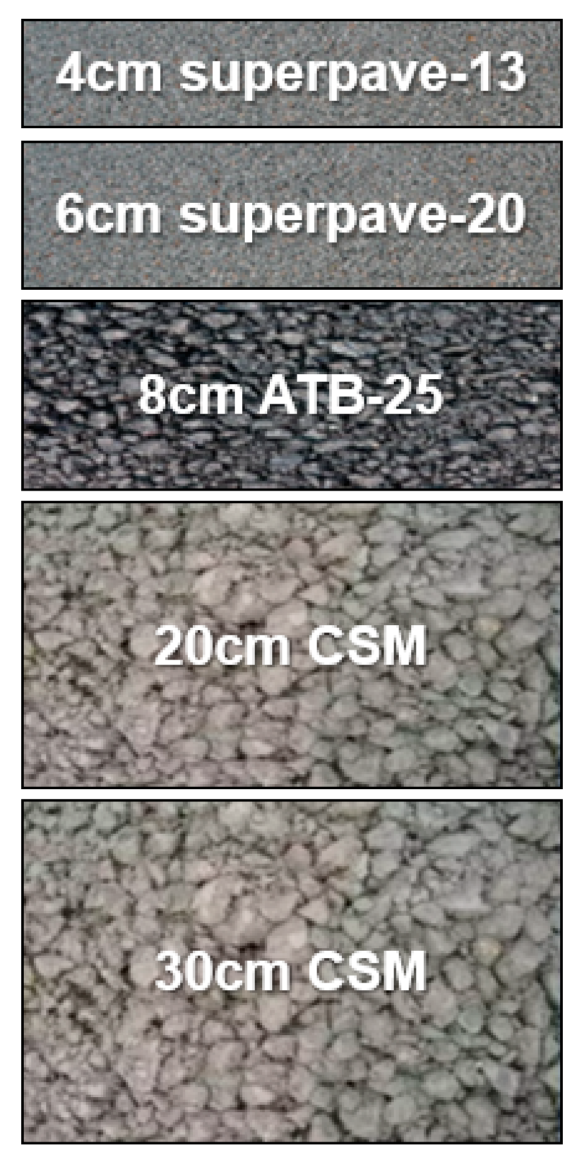
A test road was constructed and prepared for the full-size track road test. The track was designed to be a 40 km single-lane of a typical structure (4 cm + 6 cm Superpave surface course and an 8-cm asphalt-treated base) on a 50-cm cement-stabilized base (20 + 30 cm cement-stabilized macadam) (Figure 1). Twenty-five full-load trucks were used to present the accelerated test in an unfavorable season, which was in hot weather and frequent rain days during June that year. The average range of air temperature was 16–28° and there were eight days of rain over 20 testing days. The whole loading process was separated into four stages by every 5 days. After each stage, the quality parameters, such as the international roughness index (IRI), the deflection value, and the rutting depth, were collected by automatic devices. Asphalt in-field samples were cored to test their void rates and splitting strength before and after the process. As 29,820 standardized loading times were achieved in the whole test, some bumps and pits appeared at random surface areas. These positions of potential and emerged distress obtained by coring and observation are marked as the label for the model.
3.2. Data Collection and Preparation
The data related to deterioration were collected and arranged in Table 1. Thirty-four variables were chosen to build the forest.
The data can be separated into two groups, which are initial data before the test running and in-process data during the test. Some variables imply that damage has already occurred. However, when a decision was made to uncover the surface, it was found that the result was not accurate. Some variables are linear with predictions that can be accumulated by different weights, but some variables are non-linear whose margins are hard to decide. That is why an RF model is needed to improve the accuracy of predictions.
The data are collected as much as detected to avoid disregarding any small factor, which may also have influence on the predicting result. Nevertheless, some of the variables are dependent on other inputs. We prefer more information richness than data independence. This is because the RF model is very good at multicollinear problems. Besides, if there are some negative factors introduced in the model, they can be pruned in the procedure of model optimization for computing spend and model strength.
4. Methodology
As stated in the introduction, the RF model is an ensemble learning (parallel learning) model with high accuracy. Based on every decision tree, RF can avoid over-fitting and under-fitting problems by efficiently estimating variables on large databases in most classification problems [40]. Based on a bagging (an abbreviation for the bootstrap aggregation) strategy, the database is split into N groups to build and train multiple decision trees [41]. The great number of de-correlated trees can be scored by the different generated branches to balance and improve predictive performance.
4.1. Decision Trees
In the decision tree algorithm, a set of splitting rules is used to partition data features into smaller spaces with similar responses by asking simple if-else questions about each feature. Every sub-space of data presents a simpler model, which is fitted to obtain predictions. This division-and-conquer technique can produce simple rules that can easily be understood and visualized by tree diagrams. In the classification trees of this study, the gini impurity and information gain criteria are computed to evaluate the possibility and performance of each tree.
4.2. Bagging
Bootstrap aggregation or bagging is a powerful procedure to improve the bagged decision trees learning behavior to achieve low root mean squared error (RMSE) by reducing the high variance from a single-tree structure [42].
The training data can be split into multiple subsets at random, which are fitted and trained by independent decision tree models separately. The aggregation of the predictions across all the trees is averaged to minimize the correlation effects between each couple of trees. The process is shown as follows:
- (1)
- Set as the number of the generated trees;
- (2)
- Build th prediction tree model as by bootstrapping;
- (3)
- Average all predictions of trees, as shown as Expression (1) [42].
According to this procedure, though, every single tree model has high variance. The averaged B trees, which combine hundreds of trees, can reduce the value as a whole.
4.3. Out-of-the-Box Performance
For the classification problem, which has qualitative outcomes, a voting strategy is adapted to record the predicted class and pick the most frequently occurring class. It is a straightforward method to assess the error performance for a bagged prediction model.
Out-of-bag (OOB) observations are used to predict and evaluate the results by trained model. Comparing the results and observations, the classification error or test error can be accumulated.
Set the testing data space as , which has trees. The data can be presented as:
Fed T to the given RF model, we obtain another data set, such as:
Therefore,
4.4. The State-of-the-Art Method
The state-of-the-art (SOTA) methods are applied to check if the RF model can achieve the best performance in this learning work. Decision tree and support vector machines (SVM) models are selected to compare with the trained RF model. The decision tree model, which has good strength, is the base unit of the RF model. The SVM is also a high-performance classification algorithm. They are both commonly used in data mining.
Decision trees are constructed by the significance measurement of data. In addition, the SVM is built based on the liner kernel. The accuracy of the models is set to be the baseline for the comparison.
4.5. Relative Importance of Variables
Even though the structure of bagged trees grows bigger to gain significant improvement from a single tree, the whole model becomes harder to interpret. For computing the relative importance of each variable in the RF model, the importance value of each predictor in every single tree is recorded and accumulated to realize the comparison process. Thus, the most effective factor will be gained in the given predicted result. The high value of the relative importance means a significant weight in their relationships, which is a more important factor in the road deterioration process. Each variable importance can be summed by the reduction in the loss function, which is attributed to each split in a given tree.
5. Model Construction
5.1. Model Structure Design
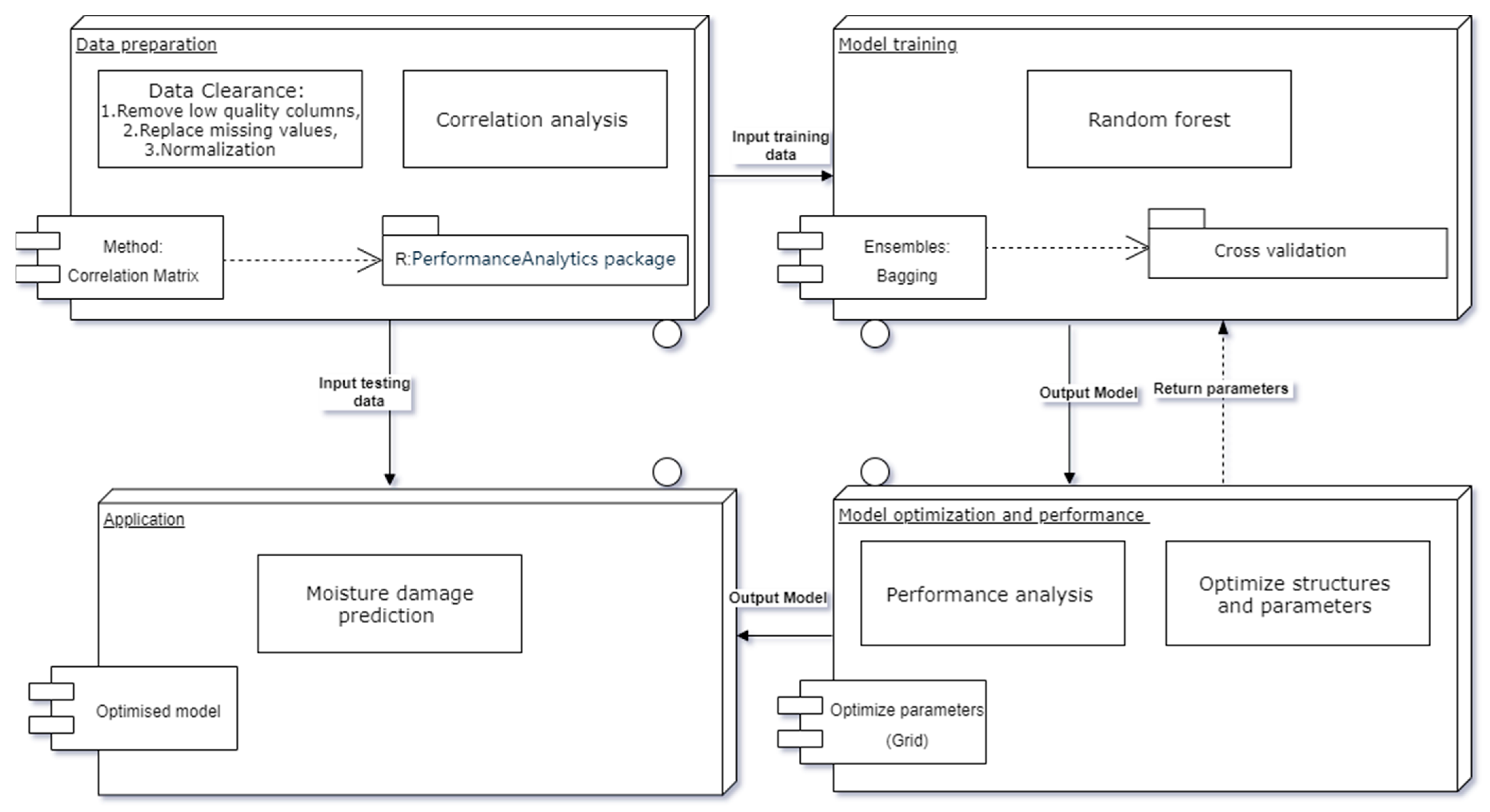
Four key steps are organized, as shown in Figure 2. A cyclic process is selected to train the RF model and optimize the model parameters repeatedly to obtain a minimal OOB error. Firstly, the quality of the given database is the most important as the basement in the whole model structure. Next, the main body of the RF model for model training is built by R language and its packages. The model will be several times to return to this step for the procedure of model optimization. This interaction of these two steps determines the final model structure and parameters, which will be applied in testing data. Finally, the prediction error rate will be estimated to assess the model performance. If insufficient performance is found, the cyclic process must run again and again after adding new data and checking the data effectiveness and correlations until achieving the best fitness of the RF model.
5.2. RF Model Construction
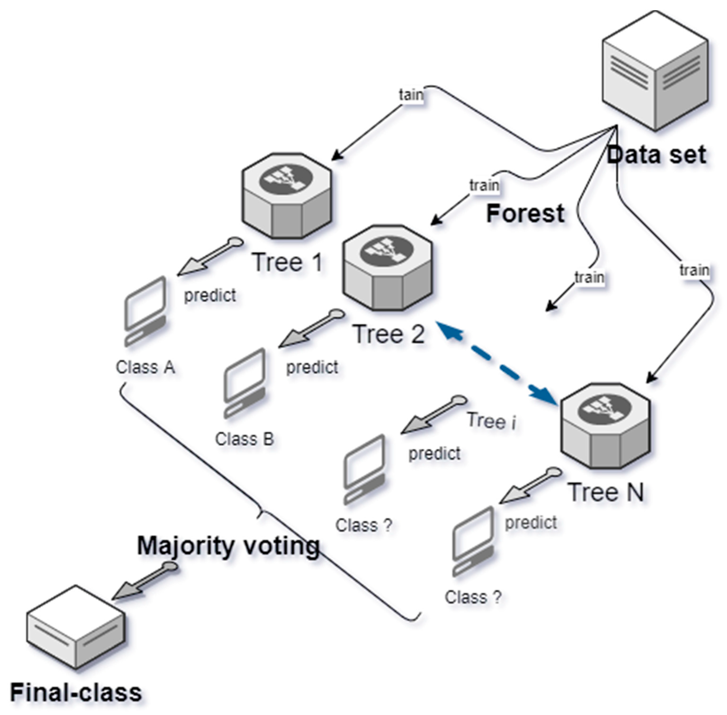
When the structure of the RF model for potential damage is decided, the training set data are input to fit and grow every single tree with two key hyperparameters, including mtry and ntree. The mtry is the number of variables tried at each split. The ntree is the total number of trees the forest will grow. To obtain classification, every tree is run down in the forest with a number m of variables, which is used to split the node. With no pruning, trees are grown as large as possible. Random forest cannot be overfit. Therefore, the number of single trees can be grown as many as the computer capability can do. With the increase in the tree number, the OOB error will keep decreasing. When all the data are run down the trees, the proximities, OOB error, and variable importance are computed. Finally, the most possible result is voted by majority voting to obtain the confident prediction. The process is shown in Figure 3.
6. Results and Discussions
6.1. Data Characteristics and Correlations
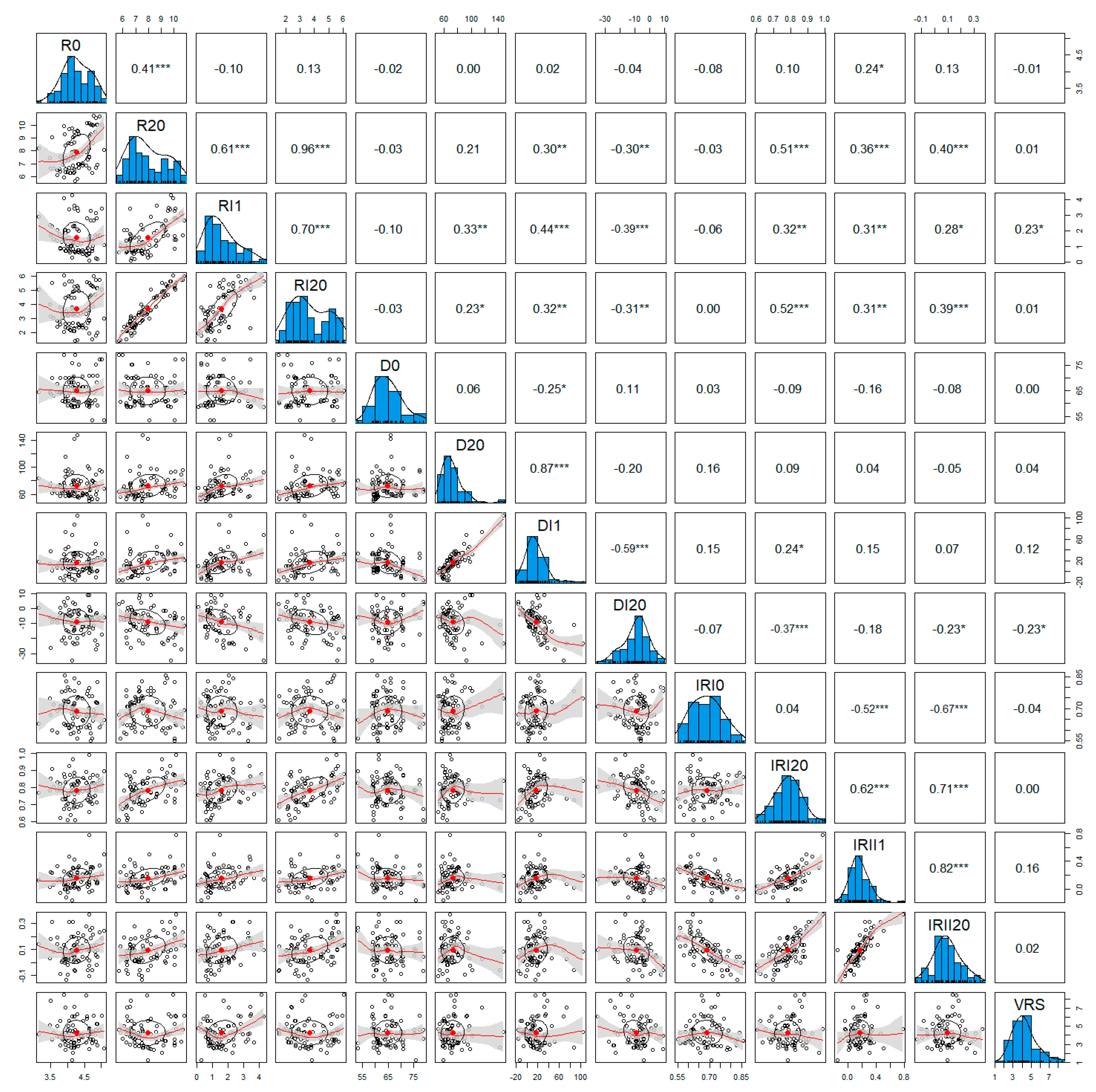
Related variables are considered as many as possible in this study for comprehensive understanding. Therefore, thirty-four categories of data about the properties of the in-field road are prepared to train. Data collection is the most important step before a model is constructed. The resources and data features are matters of the prediction results. The details of the data used in the training process cannot be exhibited due to the large data group. A general view of characters and correlations of data sets is plotted in a matrix in Figure 4.
The diagonal line of plots is the distribution status of variables, which shows that all datasets collected from road properties are almost on or can be standardized into normal distribution. Therefore, the training data are effective to work reasonably in the model. A dataset on normal distribution means it fits with the principles of the average detection data. There is no need to delete a low or abnormal variable.
The plots on the intersection between every two properties are their correlation index and fitting curves. It is clear that some of them have obvious linear correlations, which are always desirable and easy to evaluate in a typical numerical analysis. However, the other data with non-linear relationships are hard to obtain rules for. Therefore, there are no consistent principles for these factors that can determine the occurrence of potential damage. This RF model can help to combine and follow all hints of variables, even those that are not important to achieve the best prediction.
6.2. Number of Trees and Number of Variables Tried at Each Split
The two key hyperparameters, ntree and mtry, are determined by the exhaustive method. At first, an RF forest was constructed with the following default settings: ntree = 500 and mtry = 5. The OOB estimate of the error rate of the RF model is 20.24% and the confusion matrix is shown in Table 2.
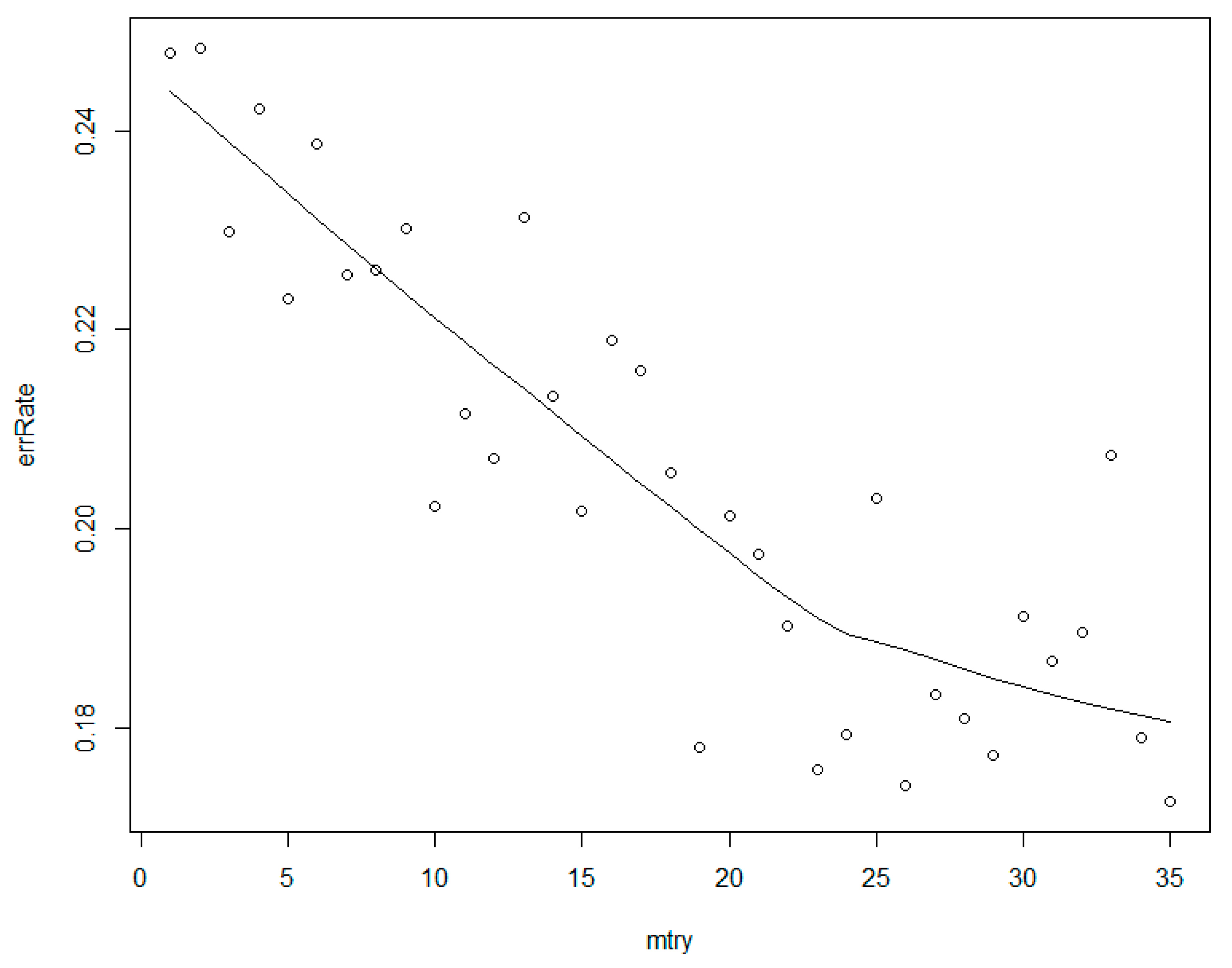
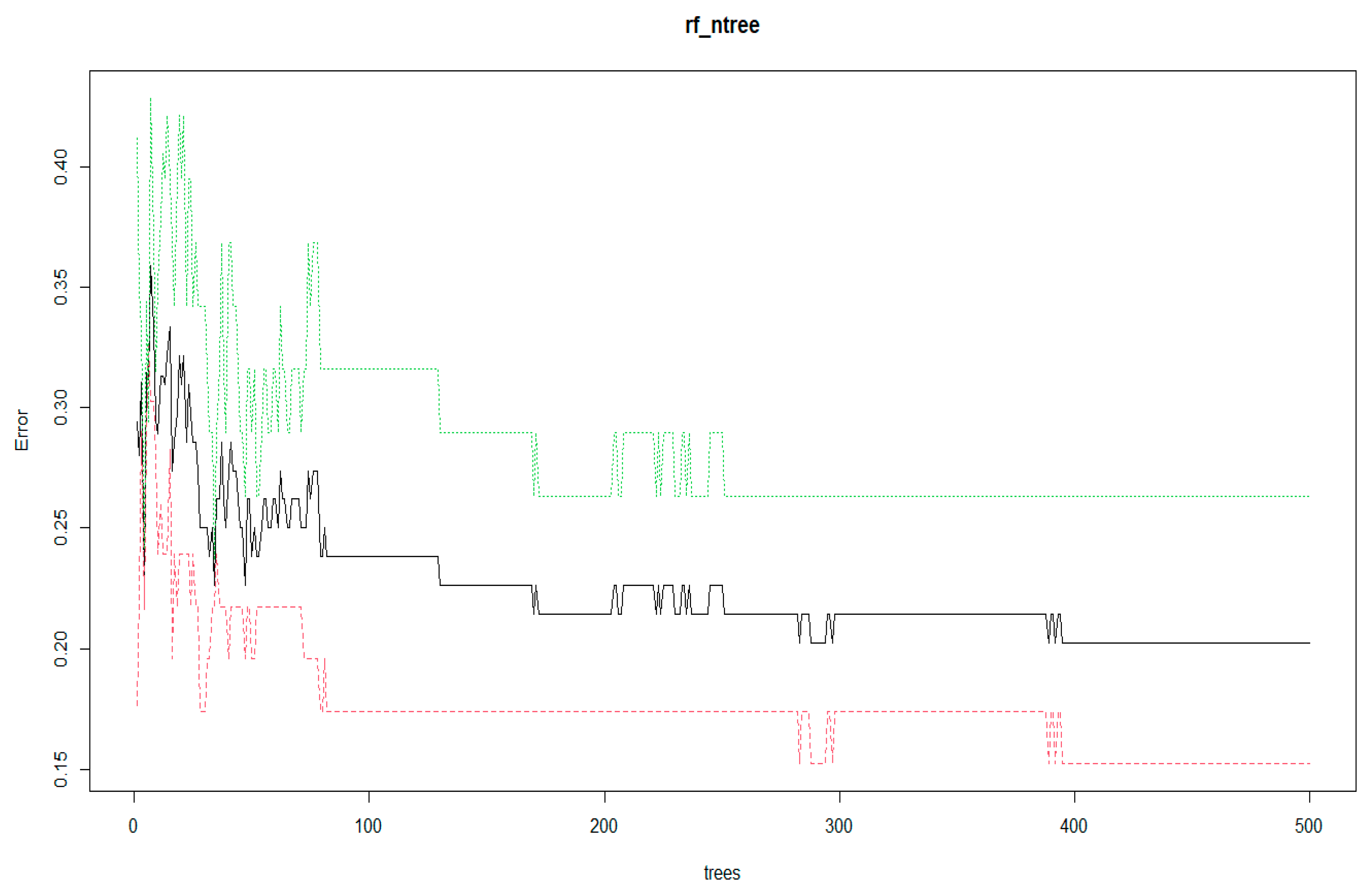
Through the exhaustive method, mtry is assigned for 1 to 35 in the default RF model with the other parameters fixed to gain the minimal error rate. According to the same method, ntree is taken to traversal algorithm again by fixing mtry value. The results and the processes are presented in Figure 5 and Figure 6.
With the increase in mtry from 1 to 35, the error rate keeps decreasing. Generally, the number of variables tried at each split in an RF model, namely the maximal deep of a tree the model grows, is random in the range between one to the number of variables. It always needs a balance for lower single-tree correlations and a certain prediction strength. Therefore, it is not a general law for an RF model as the error rate can be reduced by introducing more variables unless the variables are all effective for the model with little correlations.
In our given RF model, there are some correlated factors. This is not the main reason which affects the model accuracy until mtry equals 23. Before that, the model does not consider enough variables, which strongly helps with the increase in variables. After that or even after 19, the model is improved little when there are less independent residual factors. However, the optimal mtry value is 35 with the lowest error rate. That means that all factors have their own weights in the model even though some parts are subject to dependency.
With the increase in ntree, i.e., the number of trees generated by the model, the noise can be reduced in the model. When ntree arrives at a certain number, the error rate of the model will maintain stability. However, for the calculating speed of a computer, the best ntree value is determined. When ntree passed over 400, the prediction error rates for Y, N, and the average of the model achieved the lowest value and kept the trend. Therefore, the ntree is selected as 400 for the RF model.
6.3. The Optimized RF Model
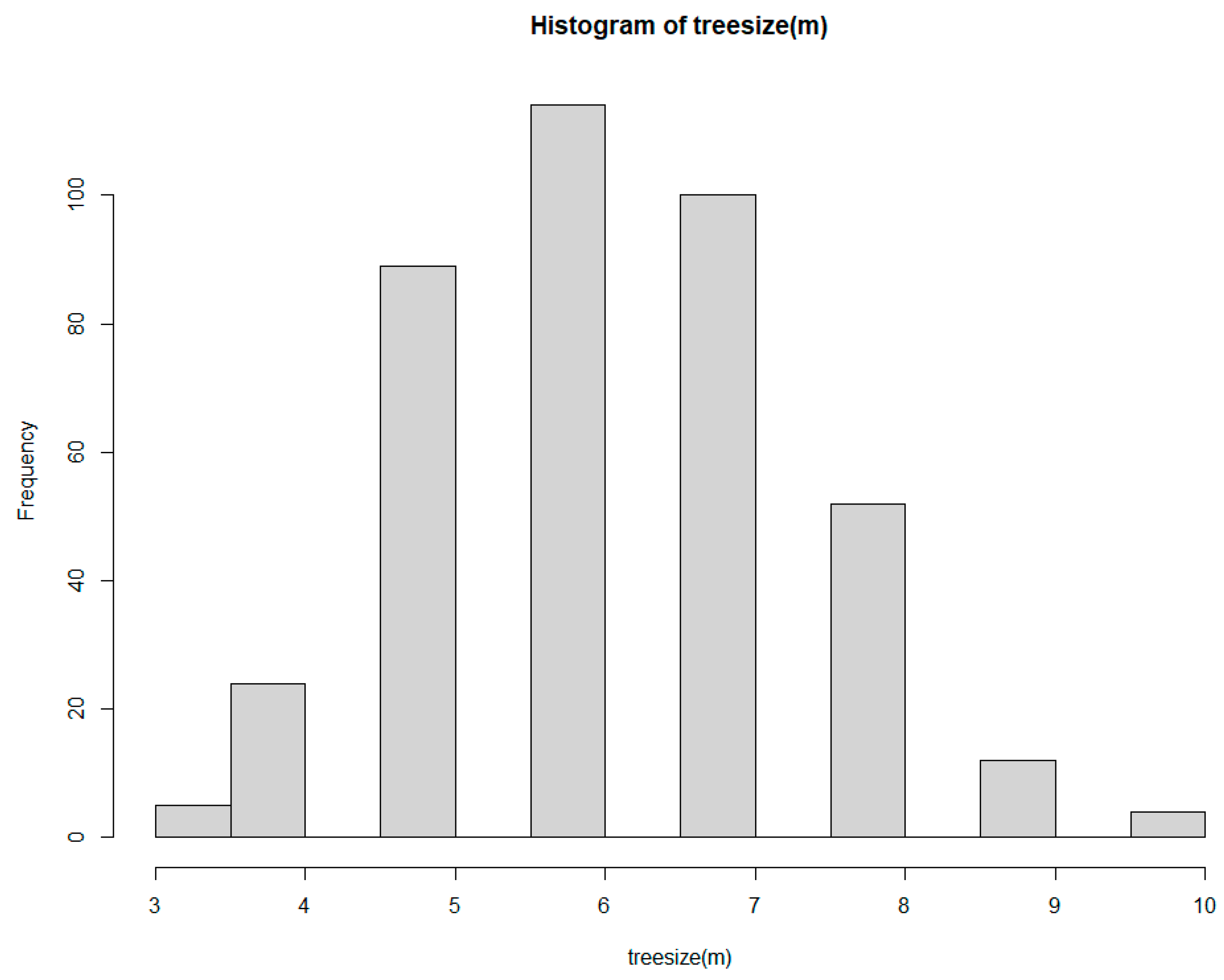
The final RF model used in training and predicting is gained through the two steps of optimization for the hyperparameters. The main tree sizes, and the node numbers of every tree in the forest, are distributed, as shown in Figure 7. The most frequent occurrence in tree sizes is six, which presents the major samples the trees in the forest look like.
The optimized RF model is estimated by the bagged testing data. The performance of the accuracy for the model is shown in matrix Table 3. The average OOB of error rate is 16.67%, which is improved greater from 20.24%. For an in-field project, prediction accuracy higher than 76% is thought to be a good performance. Compared with some other studies in highway or road topics, there are more variables in this program, which may accelerate the accuracy by considering more comprehensively. In particular, the accuracy of Y prediction, which means that the road has a potential failure at this position, has arrived at 85.13%. It is very important for road maintenance and safety in the application for saving money and lives.
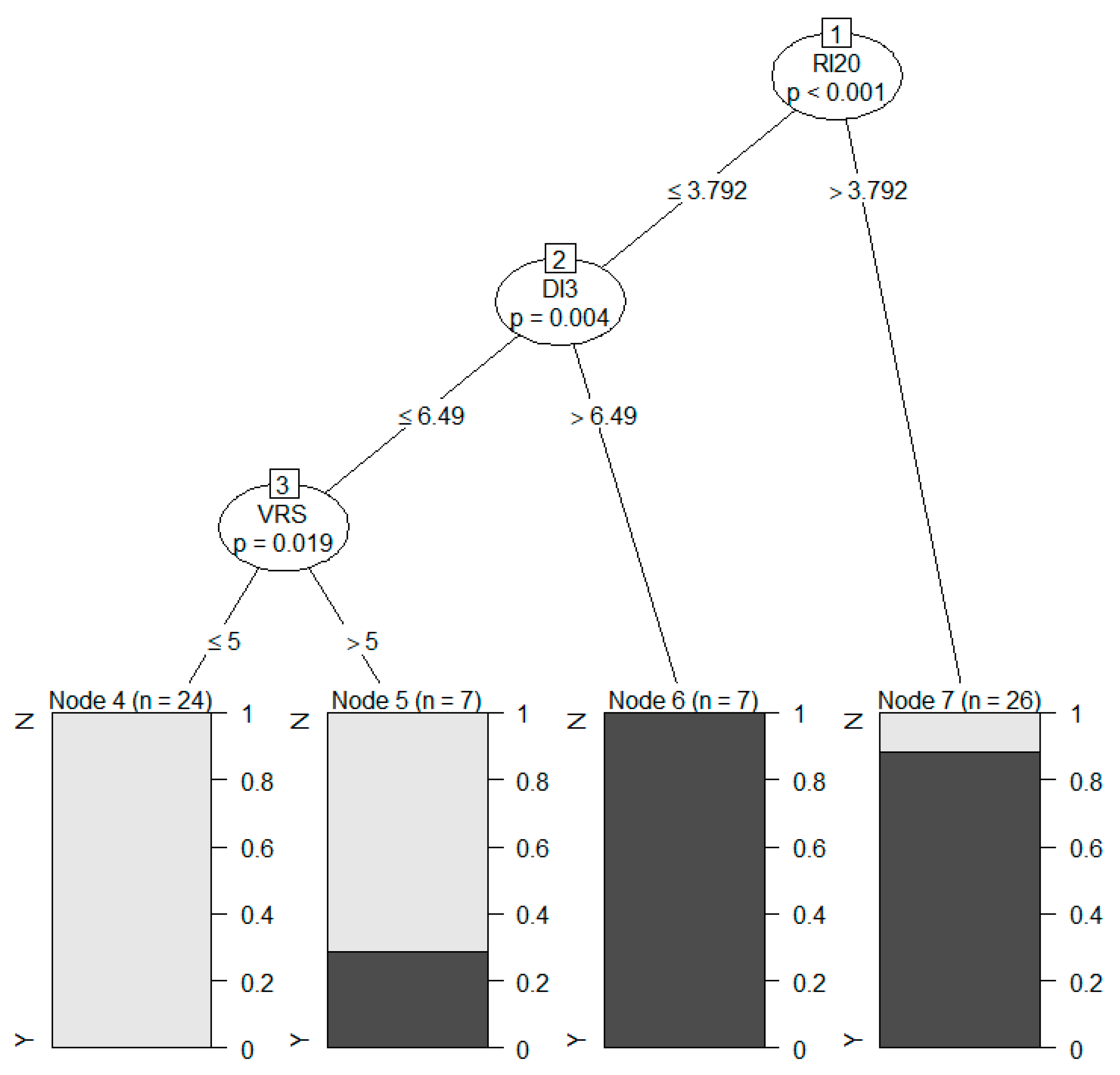
A decision tree model was constructed to compare with the RF model. The result is shown in Figure 8 and Table 4. Moreover, a support vector machine (SVM) model was built, and the relative confusion matrix is shown in Table 5.
In general, the accuracy of the decision tree model and the SVM model is 65% and 65.52%, respectively, for the separate predictions of the potential damage. Nevertheless, the decision tree model is more logical and easier to interpret. In the tree, the RI20, DI3, and VRS are the three most important factors to classify the data, and the prediction probability is given. All in all, the performance of the RF model is outstanding among the three models.
6.4. Model Application and Prediction Evaluation
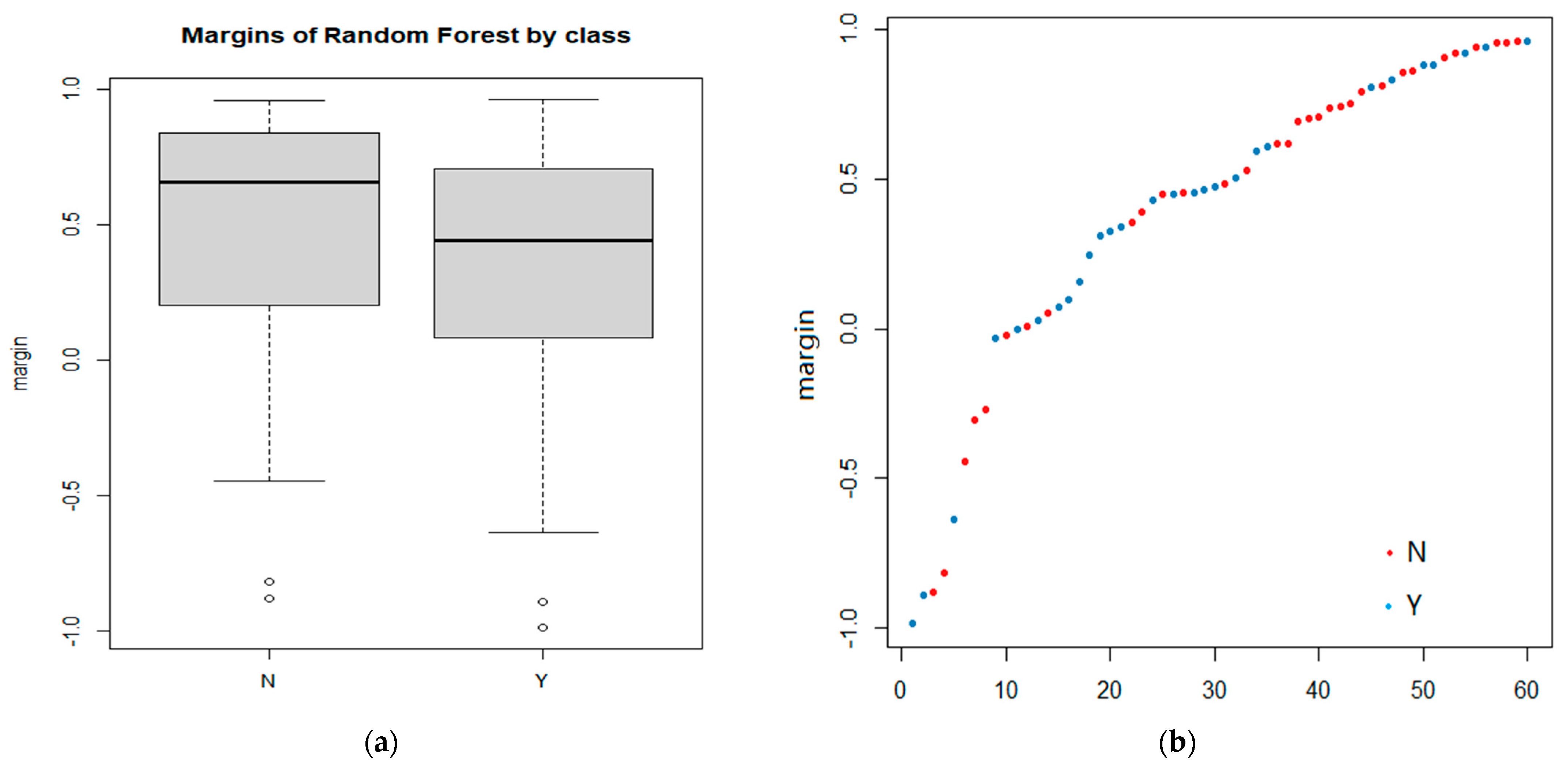
The RF model is applied and the classification performance is examined by margins and multidimensional scaling (MDS) analysis. If a margin value of a test point is higher than zero, it is identified as the right prediction. As shown in Figure 9, the prediction data meets the normal distribution. In addition, the major body of the predictions is in the upper area, which shows a good model performance, despite some abnormal points.
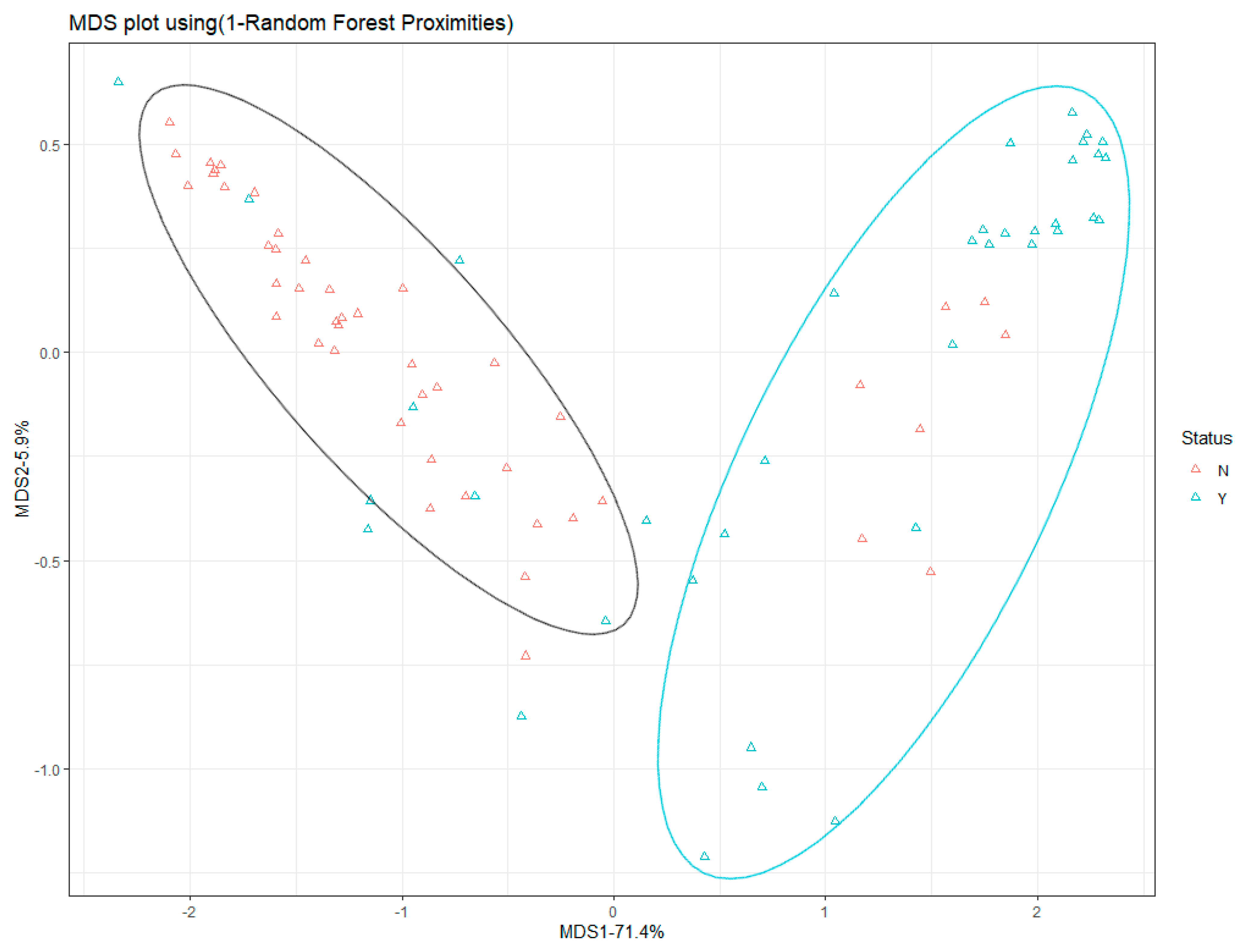
In another aspect, the MDS plot is made by R language (Figure 10). The positions of the predictions are marked in this 2D map. The predictions, especially the main bodies of Y and N predictions, have a clear boundary to each other. However, also, some points are mixed up with others, because of some inevitable abnormal points. The next step is to improve the accuracy of the detection in practice. Moreover, here, the predictions are classified into two groups, showing the classification ability of the RF model.
6.5. Factor Importance
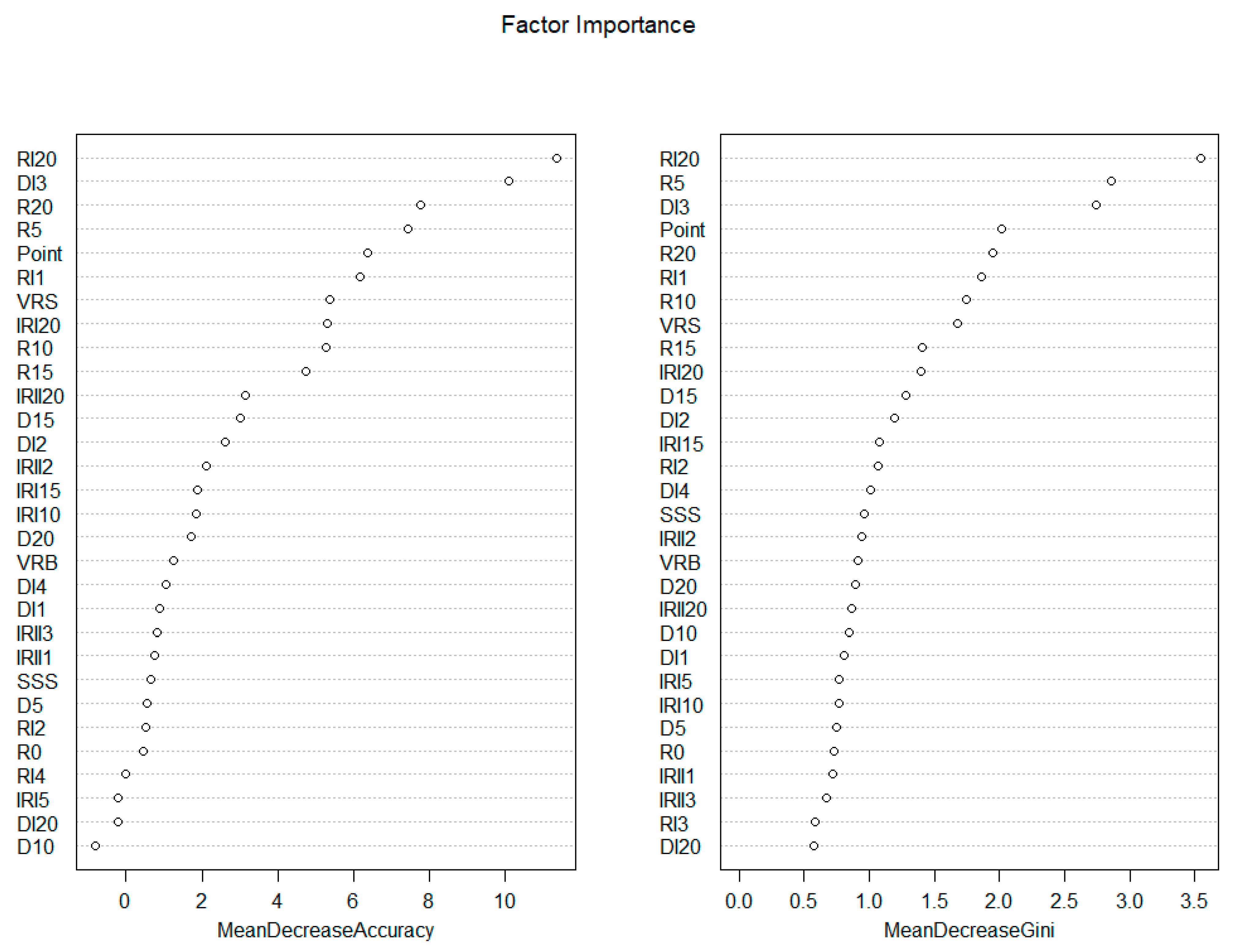
The importance of the variables is evaluated by a mean decrease in the accuracy index and a mean decrease in the Gini index for the explanation for the RF model, as shown in Figure 11. The more decrease the indexes have, the more important the factor is. The RI20, i.e., the increase in rutting over 20 days, is the most important factor, that is, if a point is rutting deeply in a short time, it is most likely to obtain moisture damage under the surface or surface failure soon. Following the RI20, i.e., the increase in deflection in the third test stage, the rutting at the 20th day and 5th day, and the position are outstanding in all variables. In these five factors, the most interesting thing is that three factors are linked to rutting, which directly presents the state of a road; a highly important factor is linked to deflection, which presents the strength of the road; and the point position is effective for predicting the project (i.e., the different construction method), which companies or materials adapted to in this road, leading this phenomenon. Based on the main important factors, it can be asserted that, before moisture damage occurs, there must firstly be a significant increase in rutting and deflection detected. Some original properties of the road, such as original rutting, original deflection, and surface splitting strength, have little weight in the model. This means that the moisture damage matters for a cumulative effect rather than the initial properties.
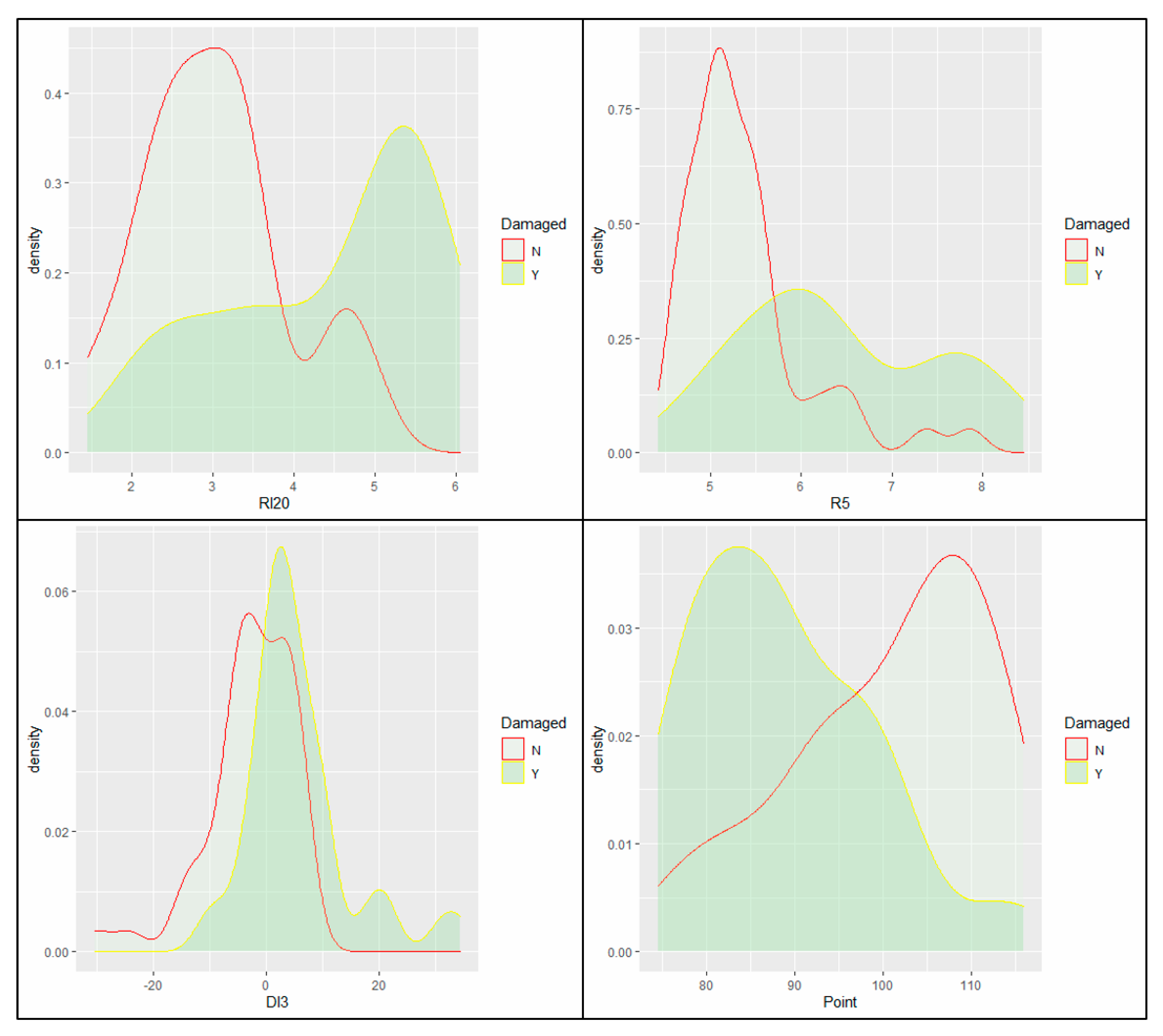
These specified values of variables and their relationships are analyzed by density curve plots. For these important variables, the overlap section of the Y and N area is smaller, which has a higher classification strength (Figure 12). Thus, it will hold a bigger weight in the model.
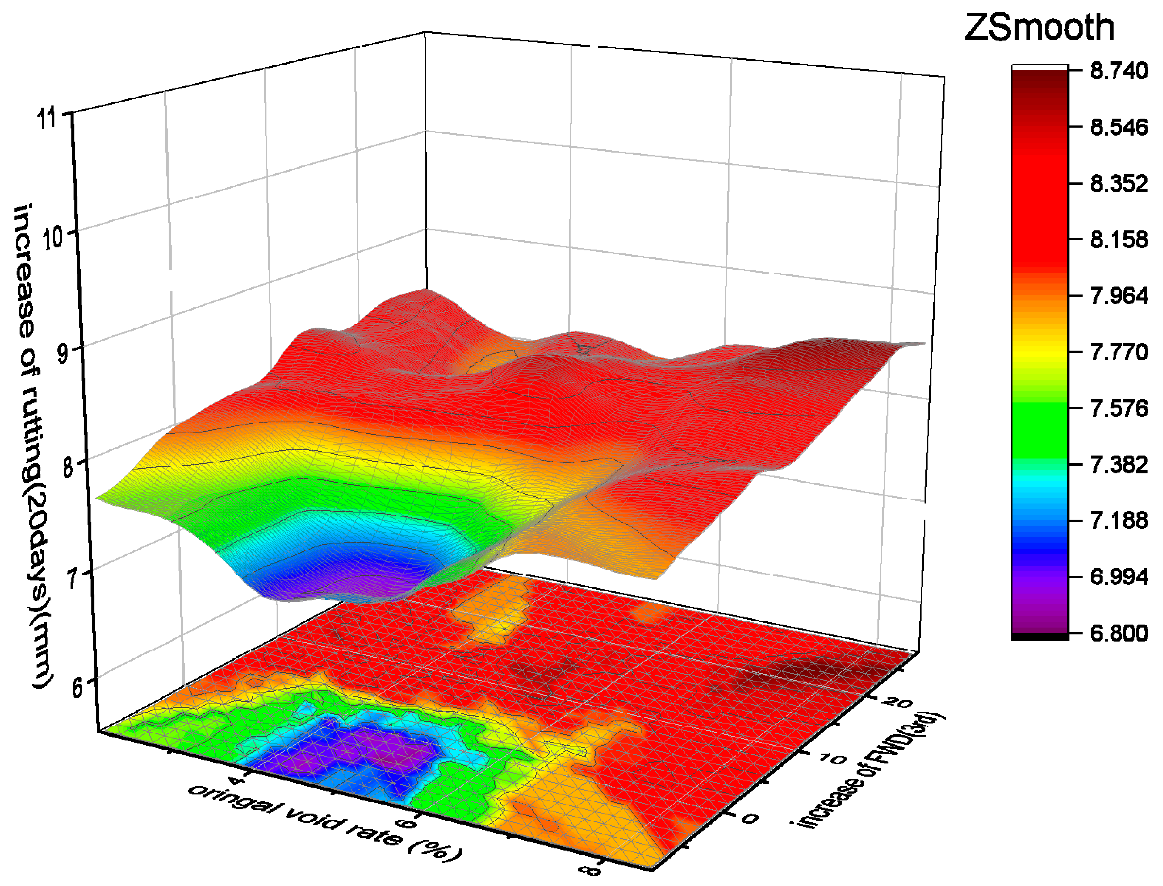
To compare the traditional analysis of properties, the three most important categories of factors from the RF model are selected for making graphics of their relationships. The void rate, the rutting increase over 20 days, and the increase in deflection in the third test stage are fitted in Figure 13.
Another interesting phenomenon is found. The void rate between 4% and 6% has the lowest probability to drop in rutting and deflection [43,44]. This finding is very similar to the Superpave construction principles. Therefore, to control the moisture damage at an early age of a road, the most important thing is to minimize construction segregation. The result proves the interpretability of the RF model, which can be easily connected to the practice work. Furthermore, the prediction of the model is rational and logical.
7. Conclusions
According to the construction and the evaluation of the RF model, a new method for predicting the potential damage is built in this article. Compared to the typical method, interrelationships of variables are analyzed through RF data mining. The excellent performance of the model is achieved with high accuracy and good interpretability by model optimization. It is concluded that:
- The RF model is suitable for the prediction of in-field properties in highway and road projects under multiple variables;
- The RF model has a good prediction accuracy and interpretability in this study;
- The optimized model can achieve a low OOB error rate of 16.67%, which can be further improved by the enhanced validity of detection data;
- The RF model and traditional method for analysis in road performance can be bridged together to obtain a more comprehensive and consistent understanding;
- The early moisture damage can be alleviated by controlling the void rate in the surface course, which is considered as a main factor by RF mining from another aspect;
- The RF model can be applied in nondestructive examination in roads for potential failure detection. In addition, by inputting more other roads’ data sets into the training, the model will become more powerful which can fit almost all situations and properties.
Author Contributions
Conceptualization, X.G. and P.H.; methodology, X.G.; validation, X.G. and P.H.; formal analysis, X.G. and P.H.; investigation, X.G.; resources, X.G.; data curation, X.G.; writing—original draft preparation, X.G.; writing—review and editing, X.G.; visualization, X.G.; supervision, P.H.; project administration, P.H.; funding acquisition, P.H. All authors have read and agreed to the published version of the manuscript.
Funding
This research received no external funding.
Institutional Review Board Statement
Not applicable.
Informed Consent Statement
Not applicable.
Data Availability Statement
The data used to support the findings of this study are available from the corresponding author upon request.
Acknowledgments
This work was supported by my supervisor, Peiwen Hao. The authors would like to thank Peiwen Hao for excellent technical support and Jinghui Hou for critically helping in my life.
Conflicts of Interest
The authors declare no conflict of interest.
References
- Transportation Research Board. Moisture Sensitivity of Asphalt Pavements: A National Seminar. In Proceedings of the TRB Committee on Bituminous–Aggregate Combinations to Meet Surface Requirements, San Diego, FL, USA, 4–6 February 2003. [Google Scholar]
- Hicks, R.G.; Program, N.C.H.R. Moisture Damage in Asphalt Concrete; Transportation Research Board: Washington, DC, USA, 1991; ISBN 978-0-309-04924-5. [Google Scholar]
- Sharaf, E.A.; Sinha, K.C. Estimation of Pavement Routine Maintenance Costs. Transp. Res. Rec. 1984, 951, 55–58. [Google Scholar]
- Underwood, B.S.; Guido, Z.; Gudipudi, P.; Feinberg, Y. Increased Costs to US Pavement Infrastructure from Future Temperature Rise. Nat. Clim. Chang. 2017, 7, 704–707. [Google Scholar] [CrossRef]
- Meneses, S.; Ferreira, A. Pavement Maintenance Programming Considering Two Objectives: Maintenance Costs and User Costs. Int. J. Pavement Eng. 2013, 14, 206–221. [Google Scholar] [CrossRef]
- Kim, S.-H.; Jeong, J.-H.; Kim, N. Use of Surface Free Energy Properties to Predict Moisture Damage Potential of Asphalt Concrete Mixture in Cyclic Loading Condition. KSCE J. Civ. Eng. 2003, 7, 381–387. [Google Scholar] [CrossRef]
- Cheng, D.; Little, D.N.; Lytton, R.L.; Holste, J.C. Use of Surface Free Energy Properties of the Asphalt-Aggregate System to Predict Moisture Damage Potential (with Discussion). J. Assoc. Asph. Paving Technol. 2002, 71, 59–88. [Google Scholar]
- Aschenbrener, T. Evaluation of Hamburg Wheel-Tracking Device to Predict Moisture Damage in Hot-Mix Asphalt. Transp. Res. Rec. 1995, 1492, 193. [Google Scholar]
- Hamzah, M.O.; Kakar, M.R.; Hainin, M.R. An Overview of Moisture Damage in Asphalt Mixtures. J. Teknol. 2015, 73, 125–131. [Google Scholar] [CrossRef] [Green Version]
- Omar, H.A.; Yusoff, N.I.M.; Mubaraki, M.; Ceylan, H. Effects of Moisture Damage on Asphalt Mixtures. J. Traffic Transp. Eng. Engl. Ed. 2020, 7, 600–628. [Google Scholar] [CrossRef]
- Ksaibati, K.; Armaghani, J.; Fisher, J. Effect of Moisture on Modulus Values of Base and Subgrade Materials. Transp. Res. Rec. 2000, 1716, 20–29. [Google Scholar] [CrossRef]
- Behiry, A.E.A.E.-M. Laboratory Evaluation of Resistance to Moisture Damage in Asphalt Mixtures. Ain Shams Eng. J. 2013, 4, 351–363. [Google Scholar] [CrossRef] [Green Version]
- Saarenketo, T.; Scullion, T. Road Evaluation with Ground Penetrating Radar. J. Appl. Geophys. 2000, 43, 119–138. [Google Scholar] [CrossRef]
- Aavik, A.; Talvik, O. Use of Falling Weight Deflectometer (Fwd) Measurement Data for Pavement Structural Evaluation and Repair Design; Federal Highway Administration: Washington, DC, USA, 2021.
- Chen, D.-H.; Xie, J.; Scullion, T. Using GPR and FWD to Assist in Selecting the Optimal Pavement Rehabilitation Strategy. In Proceedings of the GeoHunan International Conference 2011, Hunan, China, 9–11 June 2011; pp. 63–70. [Google Scholar] [CrossRef]
- Khan, Z.; Ahmed, M.; Tarefder, R. Evaluation of Pavement Performance under FWD Test through Instrumented Pavement Section. In Proceedings of the NDE/NDT for Highways & Bridges: SMT 2018, New Brunswick, OH, USA, 27–29 August 2018; pp. 192–197. [Google Scholar]
- Hoang, N.-D.; Nguyen, Q.-L. A Novel Method for Asphalt Pavement Crack Classification Based on Image Processing and Machine Learning. Eng. Comput. 2019, 35, 487–498. [Google Scholar] [CrossRef]
- Witten, I.H.; Frank, E.; Hall, M.A.; Pal, C. Mining: Practical Machine Learning Tools and Techniques; Elsevier: Amsterdam, The Netherlands, 2011; ISBN 978-0-12-374856-0. [Google Scholar]
- Zhang, X.-D. Machine Learning. In A Matrix Algebra Approach to Artificial Intelligence; Springer: Singapore, 2020; pp. 223–440. ISBN 9789811527692. [Google Scholar]
- Mahesh, B. Machine Learning Algorithms—A Review. Int. J. Comput. Sci. Inf. Technol. 2018, 9, 7. [Google Scholar]
- Naqa, E.I.; Murphy, M.J. What Is Machine Learning? In Machine Learning in Radiation Oncology; El Naqa, I., Li, R., Murphy, M.J., Eds.; Springer International Publishing: Cham, Swizterland, 2015; pp. 3–11. ISBN 978-3-319-18304-6. [Google Scholar]
- Tsai, Y.-C.; Zhao, Y.; Pop-Stefanov, B.; Chatterjee, A. Automatically Detect and Classify Asphalt Pavement Raveling Severity Using 3D Technology and Machine Learning. Int. J. Pavement Res. Technol. 2021, 14, 487–495. [Google Scholar] [CrossRef]
- Cheng, D.; Little, D.N.; Lytton, R.L.; Holste, J.C. Moisture Damage Evaluation of Asphalt Mixtures by Considering Both Moisture Diffusion and Repeated-Load Conditions. Transp. Res. Rec. J. Transp. Res. Board 2003, 1832, 42–49. [Google Scholar] [CrossRef]
- Sebaaly, P.; Tabatabaee, N.; Bonaquist, R.; Anderson, D. Evaluating Structural Damage of Flexible Pavements Using Cracking and Falling Weight Deflectometer Data. Transp. Res. Rec. 1989, 1227, 44–52. [Google Scholar]
- Karballaeezadeh, N.; Ghasemzadeh Tehrani, H.; Mohammadzadeh Shadmehri, D.; Shamshirband, S. Estimation of Flexible Pavement Structural Capacity Using Machine Learning Techniques. Front. Struct. Civ. Eng. 2020, 14, 1083–1096. [Google Scholar] [CrossRef]
- Jia, X.; Woods, M.; Gong, H.; Zhu, D.; Hu, W.; Huang, B. Evaluation of Influence of Pavement Data on Measurement of Deflection on Asphalt Surfaced Pavements Utilizing Traffic Speed Deflection Device. Constr. Build. Mater. 2021, 270, 121842. [Google Scholar] [CrossRef]
- Marcelino, P.; de Lurdes Antunes, M.; Fortunato, E.; Gomes, M.C. Machine Learning Approach for Pavement Performance Prediction. Int. J. Pavement Eng. 2021, 22, 341–354. [Google Scholar] [CrossRef]
- Gong, H.; Sun, Y.; Mei, Z.; Huang, B. Improving Accuracy of Rutting Prediction for Mechanistic-Empirical Pavement Design Guide with Deep Neural Networks. Constr. Build. Mater. 2018, 190, 710–718. [Google Scholar] [CrossRef]
- Gong, H.; Sun, Y.; Huang, B. Gradient Boosted Models for Enhancing Fatigue Cracking Prediction in Mechanistic-Empirical Pavement Design Guide. J. Transp. Eng. Part B Pavements 2019, 145, 04019014. [Google Scholar] [CrossRef]
- Jia, X.; Woods, M.; Gong, H.; Hu, W.; Huang, B.; Faraj, B. Utilization of State Performance Indices to Correlate National Performance Measures for Asphalt Pavements in Tennessee. Transp. Res. Rec. J. Transp. Res. Board 2019, 2673, 379–388. [Google Scholar] [CrossRef]
- Ham, J.; Yangchi, C.; Crawford, M.M.; Ghosh, J. Investigation of the Random Forest Framework for Classification of Hyperspectral Data. IEEE Trans. Geosci. Remote Sens. 2005, 43, 492–501. [Google Scholar] [CrossRef] [Green Version]
- Paul, A.; Mukherjee, D.P.; Chintha, R.; Kundu, S. Improved Random Forest for Classification. IEEE Trans. Image Process. 2018, 27, 4012–4024. [Google Scholar] [PubMed]
- Svetnik, V.; Liaw, A.; Tong, C.; Culberson, J.C.; Sheridan, R.P.; Feuston, B.P. Random Forest: A Classification and Regression Tool for Compound Classification and QSAR Modeling. J. Chem. Inf. Comput. Sci. 2003, 43, 1947–1958. [Google Scholar] [CrossRef] [PubMed]
- Biau, G.; Scornet, E. A Random Forest Guided Tour. TEST 2016, 25, 197–227. [Google Scholar] [CrossRef] [Green Version]
- Speiser, J.L.; Miller, M.E.; Tooze, J.; Ip, E. A Comparison of Random Forest Variable Selection Methods for Classification Prediction Modeling. Expert Syst. Appl. 2019, 134, 93–101. [Google Scholar] [CrossRef]
- Gong, H.; Sun, Y.; Hu, W.; Polaczyk, P.A.; Huang, B. Investigating Impacts of Asphalt Mixture Properties on Pavement Performance Using LTPP Data through Random Forests. Constr. Build. Mater. 2019, 204, 203–212. [Google Scholar] [CrossRef]
- Mohamed, O.A.; Ati, M.; Najm, O.F. Predicting Compressive Strength of Sustainable Self-Consolidating Concrete Using Random Forest. Key Eng. Mater. 2017, 744, 141–145. [Google Scholar] [CrossRef]
- Gong, H.; Sun, Y.; Shu, X.; Huang, B. Use of Random Forests Regression for Predicting IRI of Asphalt Pavements. Constr. Build. Mater. 2018, 189, 890–897. [Google Scholar] [CrossRef]
- Oshiro, T.M.; Perez, P.S.; Baranauskas, J.A. How Many Trees in a Random Forest? In Machine Learning and Data Mining in Pattern Recognition; Perner, P., Ed.; Lecture Notes in Computer Science; Springer: Berlin/Heidelberg, Germany, 2012; Volume 7376, pp. 154–168. ISBN 978-3-642-31536-7. [Google Scholar]
- Breiman, L. Random Forests. Mach. Learn. 2001, 45, 5–32. [Google Scholar] [CrossRef] [Green Version]
- Parmar, A.; Katariya, R.; Patel, V. A Review on Random Forest: An Ensemble Classifier. In Proceedings of the International Conference on Intelligent Data Communication Technologies and Internet of Things, Coimbatore, India, 7–8 August 2018; Springer: Berlin/Heidelberg, Germany, 2018; pp. 758–763. [Google Scholar]
- Liaw, A.; Wiener, M. Classification and Regression by RandomForest. R News 2002, 2, 18–22. [Google Scholar]
- Grant, T.P. Determination of Asphalt Mixture Healing Rate Using the Superpave Indirect Tensile Test; University of Florida: Gainesville, FL, USA, 2001. [Google Scholar]
- Christensen, D.W.; Bonaquist, R.F. Volumetric Requirements for Superpave Mix Design; Transportation Research Board: Washington, DC, USA, 2006; Volume 567, ISBN 0-309-09867-X. [Google Scholar]
Figure 1.
The structure of the test road.

Figure 2.
Structure design of the RF model.

Figure 3.
RF model construction process.

Figure 4.
Data characteristics and correlations matrix: the * represents the significance level.

Figure 5.
The relationship between mtry and the error rate.

Figure 6.
The relationship between ntree and the error rate.

Figure 7.
The tree size and its occurrence frequency.

Figure 8.
The decision tree model.

Figure 9.
The margins of the RF model by class: (a) the margins of outputs checking the classification performance; (b) the outputs mapping from multiple dimensional data to 2 dimensions.
Figure 9.
The margins of the RF model by class: (a) the margins of outputs checking the classification performance; (b) the outputs mapping from multiple dimensional data to 2 dimensions.

Figure 10.
The MDS of the RF model.

Figure 11.
Factor importance.

Figure 12.
Specified values of variables and their relationships.

Figure 13.
The relationships amongst the three important factors.


Table 1.
Description of variables.
| Variables | Symbol | Unit |
|---|---|---|
| The original rutting depth | R0 | mm |
| The rutting depth on the fifth day | R5 | mm |
| The rutting depth on the tenth day | R10 | mm |
| The rutting depth on the fifteenth day | R15 | mm |
| The rutting depth on the twentieth day | R20 | mm |
| Increase in rutting depth at the first stage of the test | RI1 | mm |
| Increase in rutting depth in the second stage of the test | RI2 | mm |
| Increase in rutting depth in the third stage of the test | RI3 | mm |
| Increase in rutting depth in the fourth stage of the test | RI4 | mm |
| Increase in rutting depth through the whole test | RI20 | mm |
| The original deflection value | D0 | 0.001 mm |
| The deflection value on the fifth day | D5 | 0.001 mm |
| The deflection value on the tenth day | D10 | 0.001 mm |
| The deflection value on the fifteenth day | D15 | 0.001 mm |
| The deflection value on the twentieth day | D20 | 0.001 mm |
| Increase in the deflection value in the first stage of the test | DI1 | 0.001 mm |
| Increase in the deflection value in the second stage of the test | DI2 | 0.001 mm |
| Increase in the deflection value in the third stage of the test | DI3 | 0.001 mm |
| Increase in the deflection value in the fourth stage of the test | DI4 | 0.001 mm |
| Increase in the deflection value through the whole test | DI20 | 0.001 mm |
| The original IRI value | IRI0 | m/km |
| The IRI value on the fifth day | IRI5 | m/km |
| The IRI value on the tenth day | IRI10 | m/km |
| The IRI value on the fifteenth day | IRI15 | m/km |
| The IRI value on the twentieth day | IRI20 | m/km |
| Increase in the IRI value in the first stage of the test | IRII1 | m/km |
| Increase in the IRI value in the second stage of the test | IRII2 | m/km |
| Increase in the IRI value in the third stage of the test | IRII3 | m/km |
| Increase in the IRI value in the fourth stage of the test | IRII4 | m/km |
| Increase in the IRI value through the whole test | IRII20 | m/km |
| The void rate of the surface course | VRS | % |
| The void rate of the bottom ATB | VTB | % |
| The splitting strength of the surface course | SSS | Mpa |
| The splitting strength of the bottom ATB | SSB | Mpa |
Table 2.
Confusion matrix of the default RF model.
| Ture N | Ture Y | Class. Error | |
|---|---|---|---|
| Pred. N | 39 | 7 | 0.1521739 |
| Pred. Y | 10 | 28 | 0.2631579 |
Y presents the points marked as distress; N presents the points marked as in good condition.
Table 3.
Confusion matrix of the optimized RF model.
| Ture N | Ture Y | Class. Error | |
|---|---|---|---|
| Pred. N | 26 | 6 | 0.1875000 |
| Pred. Y | 4 | 24 | 0.148671 |
Y presents the points marked as distress; N presents the points marked as in good condition.
Table 4.
Confusion matrix of the decision tree model.
| Ture N | Ture Y | Class. Error | |
|---|---|---|---|
| Pred. N | 10 | 3 | 0.230769 |
| Pred. Y | 4 | 3 | 0.571428 |
Y presents the points marked as distress; N presents the points marked as in good condition.
Table 5.
Confusion matrix of the SVM model.
| Ture N | Ture Y | Class. Error | |
|---|---|---|---|
| Pred. N | 10 | 7 | 0.411765 |
| Pred. Y | 3 | 9 | 0.250000 |
Y presents the points marked as distress; N presents the points marked as in good condition.
Publisher’s Note: MDPI stays neutral with regard to jurisdictional claims in published maps and institutional affiliations. |
© 2021 by the authors. Licensee MDPI, Basel, Switzerland. This article is an open access article distributed under the terms and conditions of the Creative Commons Attribution (CC BY) license (https://creativecommons.org/licenses/by/4.0/).
Share and Cite
MDPI and ACS Style
Guo, X.; Hao, P. Using a Random Forest Model to Predict the Location of Potential Damage on Asphalt Pavement. Appl. Sci. 2021, 11, 10396. https://doi.org/10.3390/app112110396
AMA Style
Guo X, Hao P. Using a Random Forest Model to Predict the Location of Potential Damage on Asphalt Pavement. Applied Sciences. 2021; 11(21):10396. https://doi.org/10.3390/app112110396
Chicago/Turabian StyleGuo, Xiaogang, and Peiwen Hao. 2021. "Using a Random Forest Model to Predict the Location of Potential Damage on Asphalt Pavement" Applied Sciences 11, no. 21: 10396. https://doi.org/10.3390/app112110396
Note that from the first issue of 2016, this journal uses article numbers instead of page numbers. See further details here.