Image Retrieval Method Based on Image Feature Fusion and Discrete Cosine Transform

Abstract

This paper presents a new content-based image retrieval (CBIR) method based on image feature fusion. The deep features are extracted from object-centric and place-centric deep networks. The discrete cosine transform (DCT) solves the strong correlation of deep features and reduces dimensions. The shallow features are extracted from a Quantized Uniform Local Binary Pattern (ULBP), hue-saturation-value (HSV) histogram, and dual-tree complex wavelet transform (DTCWT). Singular value decomposition (SVD) is applied to reduce the dimensions of ULBP and DTCWT features. The experimental results tested on Corel datasets and the Oxford building dataset show that the proposed method based on shallow features fusion can significantly improve performance compared to using a single type of shallow feature. The proposed method based on deep features fusion can slightly improve performance compared to using a single type of deep feature. This paper also tests variable factors that affect image retrieval performance, such as using principal component analysis (PCA) instead of DCT. The DCT can be used for dimensional feature reduction without losing too much performance.

1. Introduction

As the amount of available data grows, the explosion of images has brought significant challenges to automated image search and retrieval. While the explosive growth of internet data provides richer information and more choices, it also means that users need to browse an ever-increasing amount of content to retrieve the desired results. Therefore, effectively integrating multiple-media information on the internet to assist users in quick and efficient retrieval has become a new hot issue in image retrieval.

Traditional image retrieval technology is mainly divided into text-based image retrieval and content-based image retrieval [1]. Text-based image retrieval [2] first requires manual annotation or machine learning to generate corresponding text annotations for the images in a database, then calculates the distance between the annotations and query words and sorts them in ascending order to produce a search list. Text-based retrieval is still the primary retrieval method used by various retrieval machines today. Its main advantage is that it can retrieve related images quickly. Still, its disadvantage is that the text information contains more irrelevant information. It is easy to produce many irrelevant images in the search results, which affects search accuracy. Additionally, the workload of manual labeling is large, and it is not easy to provide appropriate text labels for all the new pictures generated every day. The primary mechanism of content-based image retrieval technology is to extract various visual features of a query image [3]. A set of visually similar results to the query image is retrieved and returned to the user through feature matching with an image in a database. Content-based image retrieval technology works by matching visual image information, avoids the heavy workload of manual marking, and provides retrieval results that can meet users’ needs in terms of visual features. Because this method is based on the measurement of similarity between images, it can retrieve images similar to the target sample in the query image for the user. The accuracy of the results obtained by the image search engine query based on text annotation is often not ideal, so the research community favors content-based image retrieval.

The visual characteristics of images such as color, texture, and shape are widely used for image indexing and retrieval. In recent years, various content-based image retrieval methods have sprung up. Color is the most used feature in image retrieval, and its definition is related to the color space used by the image. A color space [4] is a method of describing the space selected by a computer according to the needs of different scenes, including RGB, CIE 1931 XYZ color space, YUV, HSV, CMYK, and so on. The use of color features to describe images usually requires the combination of color distribution histogram technology. A statistical color distribution histogram structure is established to express color distribution and local spatial structure information by identifying the color information in a structure window. An HSV histogram [5] is used extensively in CBIR, offering better-colored images than grayscale images. Since human vision is more sensitive to brightness than to color intensity, the human visual system often uses the HSV color space, which is more in line with human visual characteristics than the RGB color space, to facilitate color processing and recognition. The modified color motif co-occurrence matrix (MCMCM) [6] collects the inter-correlation between the red, green, and blue color planes, absent in the color motif co-occurrence matrix. Typical color statistical features also include the color covariance matrix, color aggregation vector, color coherence vector (CCV) [7], and so on.

Texture features can represent the internal spatial structure information of images. The most used is the LBP [8]; the standard LBP encodes the relationship between a reference pixel and its surrounding neighbors by comparing gray-level values. Inspired by its recognition accuracy and simplicity, several variants of LBPs have been proposed. The local tetra patterns (LTrPs) [9] encode the relationship between the center pixel and its neighbors by using first-order derivatives in vertical and horizontal directions. The directional local extrema patterns (DLEP) [10] extract directional edge information based on local extrema in 0°, 45°, 90°, and 135° directions in an image. In addition, CBIR methods derived from wavelet-based texture features from Gabor wavelets [11], discrete wavelet transforms (DWT) [12], DTCWT [13], and shape-adaptive discrete wavelet transforms (SA-DWT) [14] have been studied. SA-DWT can work on each image region separately and preserve its spatial and spectral properties.

The extraction of shape features is mainly performed to capture the shape attributes (such as bending moment, area and boundary, etc.) of an image item. Efficient shape features must present essential properties such as identifiability, translation, rotation, scale-invariance, affine invariance, noise resistance, occultation independence, and reliability [15]. Shape-based methods are grouped into region-based and counter-based techniques. Methods such as Fourier descriptors [16] and geometric moments [17] are often used.

Local descriptors such as scale-invariant feature transform (SIFT) [18], speeded up robust features (SURF) [19], histograms of oriented gradient (HOG) [20], gist scene descriptors [21], and so on, are also available for image retrieval. These descriptors are mainly invariant to geometrical transformations but have high computational complexity.

Some ways to extract image feature descriptors are by using a compression scheme. The vector quantization (VQ) [22] works by dividing a large set of vectors into groups with approximately the same number of points closest to them. Quantization introduces two problems: information about the original descriptor is lost, and corresponding descriptors may be assigned to different visual words [23]. The ordered dither block truncation coding (ODBTC) [24] compresses an image block into corresponding quantizers and bitmap images. The dither array in the ODBTC method substitutes the fixed average value as the threshold value for bitmap image generation.

Image features can be roughly divided into two categories according to the ability to describe image semantics: shallow and deep features. Image retrieval based on deep features has become a hot research field with increased image data sets. Deep learning techniques allow a system to learn features with a CNN architecture. CNN-based techniques are also incorporated to extract image features at various scales and are encoded using a bag of words (BoW) [25] or vector of locally aggregated descriptors (VLAD) [26]. Recently, some CNN-based CBIR methods have been proposed. ENN-BR [27] embedded neural networks with band letized regions. LeNetF6 [28] extracted the fully connected F6 of the LeNet network [29] as the feature; shape-based filtering. SBF-SMI-CNN [30] integrated spatial mapping with CNN. The dimension reduction-based methods [31] use multilinear principal component analysis (MPCA) to reduce the dimensionality of image features.

The use of a shallow function to distinguish between different images has some limitations. Therefore, many methods based on the fusion of several shallow features have been proposed, such as CCM and the difference between pixels in a scan pattern (CCM-DBPSP) [32], color histogram and local directional pattern (CH-LDP) [33], color-shape, and a bag of words (C-S-BOW) [34], microstructure descriptor and uniform local binary patterns (MSD-LDP) [35], and correlated microstructure descriptor (CMSD) [36]. CMSD is used for correlating color, texture orientation, and intensity information. The fused information feature-based image retrieval system (FIF-IRS) [37] is composed of an eight-directional gray level co-occurrence matrix (8D-GLCM) and HSV color moments (HSVCM) [38].

The existing image retrieval methods based on CNN features are primarily used in the context of supervised learning. However, in an unsupervised context, they also have problems such as only being object-centric without considering semantic information such as location, and deep features have large dimensions. The proposed method combines deep and shallow feature fusion. The method extracts the deep features from object-centric and place-centric pre-trained networks, respectively. DCT [39] is used for deep feature reduction. The shallow features are based on HSV, LBP, and DTCWT. Singular value decomposition (SVD) [40] is applied to LBP and DTCWT for dimension reduction [41].

Our contributions include:

• An image retrieval method based on CNN-DCT is proposed. Through DCT, the correlation of CNN coefficients can be reduced. DCT has good energy accumulation characteristics and can still maintain performance during dimensionality reduction.
• A combination of shallow and deep feature fusion methods is used. Deep features are extracted from a deep neural network centered on objects and places. It has better image retrieval performance than using a single CNN feature.
• Other factors that affect the experimental results are analyzed, such as measurement metrics, neural network model structure, feature extraction location, feature dimensionality reduction methods, etc.

The remainder of the paper is organized as follows. Section 2 is an overview of related work. Section 3 introduces the proposed image retrieval method based on shallow and deep features fusion. Section 4 introduces the evaluation metrics and presents the experimental results on the Corel dataset and Oxford building dataset. Section 5 offers our conclusions.

2. Related Work

2.1. HSV Color Space and Color Quantization

HSV is an alternative representation of the RGB color model and aims to be more closely aligned with how human vision perceives color attributes. The hue component describes the color type, and saturation is the depth or purity of color. The colors of each hue are arranged in radial slices around a central axis of neutral colors, and the neutral colors range from black at the bottom to white at the top. An HSV color space is given with hue HV ∈ [0°, 360°], saturation SV ∈ [0, 1], and value V ∈ [0, 1]. The color conversion from RGB to HSV is given by [42]:

$$R,G,B\in \left[0,1\right]$$

(1)

$$X_{max}=V=\max \left(R,G,B\right)$$

(2)

$$X_{min}=\min \left(R,G,B\right)$$

(3)

$$C=X_{max}-X_{min}$$

(4)

$$H=\{\begin{array}{cc}\begin{array}{c}0\\ {60}^{°}·\left(0+\frac{G-B}{C}\right)\end{array}& \begin{array}{c}if C=0\\ if V=R\end{array}\\ \begin{array}{c}{60}^{°}·\left(2+\frac{B-R}{C}\right)\\ {60}^{°}·\left(4+\frac{R-G}{C}\right)\end{array}& \begin{array}{c}if V=G\\ if V=B\end{array}\end{array}$$

(5)

$$S_V=\{\begin{array}{cc}0& if V=0\\ \frac{C}{V}& otherwise\end{array}$$

(6)

For example, [R = 1, G = 0, B = 0] can be represented by [H = 0°, S = 1, V = 1] in HSV color. When S = 0 and V = 1, the color is white; and when V = 0, the color is black. The H, S, and V channels are divided into different bins, and then a color histogram is used for color quantization.

2.2. HSVCM Features

Moments are well known for their application in image analysis since they can be used to derive invariants concerning specific transformation classes. Color moments are scaling and rotation invariant. It is usually the case that only the first three-color moments are used as features in image retrieval applications, as most of the color distribution information is contained in the lower-order moments [38]. The color moment that symbolizes the global color details can be derived from any color space. The (p + q) order moments of a given image f(x, y) with the size of M × N can be defined by:

$$m_{pq}={{\displaystyle \sum }}_{x=1}^M{{\displaystyle \sum }}_{y=1}^N{x}^p{y}^{q}f\left(x,y\right)$$

(7)

Based on the zeroth-order moment of the image, the average value, standard deviation, and skewness from each HSV component are calculated. The color moment generates a nine-dimensional feature vector.

$$Mea{n}_{cm}=\frac{1}{M\times N}{{\displaystyle \sum }}_{x-1}^M{{\displaystyle \sum }}_{y-1}^N{F}_{cc}\left(x,y\right),cc=\left\{H,S,V\right\}$$

(8)

$$Standard Deviatio{n}_{cm}={\left[\frac{1}{M\times N}{{\displaystyle \sum }}_{x-1}^M{{\displaystyle \sum }}_{y-1}^N{F}_{cc}{\left(x,y\right)}^2\right]}^{\frac{1}{2}},cc=\left\{H,S,V\right\}$$

(9)

$$Skewnes{s}_{cm}={\left[\frac{1}{M\times N}{{\displaystyle \sum }}_{x-1}^M{{\displaystyle \sum }}_{y-1}^N{F}_{cc}{\left(x,y\right)}^3\right]}^{\frac{1}{3}},cc=\left\{H,S,V\right\}$$

(10)

where cm holds the moments of each color channel of an image. M and N are the rows and column sizes of an image. Fcc(i, j) specifies the pixel intensity of the ith row and jth column of the fastidious color channel.

2.3. Quantized LBP Features

A valuable extension of the original $LB{P}_{P, R}^{ri{u}^2}$ operator is the so-called uniform mode [43] that selects the binary mode that is more common in texture images by reducing the length of the feature vector and implementing simple rotation-invariant descriptors, where parameter P controls the quantization of the angular space, and R determines the spatial resolution of the operator. If the binary mode contains at most two 0/1 transitions, it is called a unified mode. For example, 01000000₂ (two transitions) is a uniform pattern, but 01010101₂ (seven transitions) is not. In the computation of the LBP histogram, the histogram has a separate bin for every uniform pattern, and all non-uniform patterns are assigned to a single bin. The LBP_{P, R} operator produces 2^P different output values, corresponding to the 2^P different binary patterns formed by the P pixels in the neighbor set. Using uniform patterns, the length of the feature vector for a single cell reduces from 256 to 59 by:

$$2^P\to P\times \left(P-1\right)+2+1$$

(11)

where “1” comprising all 198 non-uniform LBPs and “2” corresponding to the two unique integers 0 and 255 provide a total of 58 uniform patterns.

The quantized LBP patterns are further grouped into local histograms. The image is divided into multiple units of a given size. The quantized LBP is then aggregated into a histogram using bilinear interpolation along two spatial dimensions.

2.4. DTCWT Features

DTCWT is a relatively recent enhancement of the DWT, with nearly shift-invariant and directionally selective properties in two and higher dimensions [44]. The DWT replaces the infinitely oscillating sinusoidal basis functions of the Fourier transform with a set of locally oscillating basis functions, i.e., wavelets. Any finite energy analog signal x(t) can be decomposed in terms of wavelets and scaling operations via:

$$x\left(t\right)={{\displaystyle \sum }}_{n=-\infty }^{+\infty }c\left(n\right)\varnothing \left(t-n\right)+{{\displaystyle \sum }}_{j=0}^{\infty }{{\displaystyle \sum }}_{n=-\infty }^{\infty }d\left(j,n\right)2^{\raisebox{1ex}{$j$}\!\left/ \!\raisebox{-1ex}{$2$}\right.}\psi \left(2^{j}t-n\right)$$

(12)

where ψ(t) is the real-valued bandpass wavelet and ∅(t) is a real-valued lowpass scaling function. The scaling coefficients c(n) and wavelet coefficients d(j, n) is computed via the inner products:

$$c\left(n\right)={{\displaystyle \int }}_{-\infty }^{\infty }x\left(t\right)\varnothing \left(t-n\right)dt$$

(13)

$$d\left(j,n\right)=2^{\raisebox{1ex}{$j$}\!\left/ \!\raisebox{-1ex}{$2$}\right.}{{\displaystyle \int }}_{-\infty }^{\infty }x\left(t\right)\psi \left(2^{j}t-n\right)dt$$

(14)

The DTCWT employs two real DWTs; the first DWT gives the real part of the transform, while the second DWT gives the imaginary part. The two real wavelet transforms use two different sets of filters, with each satisfying the perfect reconstruction conditions. The two sets of filters are jointly designed so that the overall transform is approximately analytic. If the two real DWTs are represented by the square matrices F_h and F_g, the DTCWT can be represented by a rectangular matrix:

$$F=\left[\begin{array}{c}{F}_h\\ F_g\end{array}\right]$$

(15)

The complex coefficients can be explicitly computed using the following form:

$$F_c=\frac{1}{2}\left[\begin{array}{cc}I& jI\\ I& -jI\end{array}\right]·\left[\begin{array}{c}{F}_h\\ F_g\end{array}\right]$$

(16)

$$F_c^{-1}=\frac{1}{2}\left[\begin{array}{cc}{F}_h^{-1}& F_g^{-1}\end{array}\right]·\left[\begin{array}{cc}I& I\\ -jI& jI\end{array}\right]$$

(17)

CWT is applied to a complex signal, then the output of both the upper and lower filter banks will be complex.

2.5. SVD

SVD is a factorization of a real or complex matrix that generalizes the eigendecomposition of a normal square matrix to any m × n matrix M via an extension of the polar decomposition. The singular value decomposition has many practical uses in statistics, signal processing, and pattern recognition. The SVD of an m × n matrix is often denoted as UΣV^T, where “U” is an m × m unitary matrix, “Σ” is an m × n rectangular diagonal matrix with non-negative real numbers on the diagonal, and V is an n × n orthogonal square matrix. The singular values δ_i = Σ_ii of the matrix are generally chosen to form a non-increasing sequence:

$${\delta }_1\ge {\delta }_2\ge \cdots \ge {\delta }_N\ge 0$$

(18)

The number of non-zero singular values is equal to the rank of M. The columns of U and V are called the left-singular vectors and right-singular vectors of M, respectively. A non-negative real number σ is a singular value for M if and only if there exist unit-length vectors u in K^m and v in Kⁿ:

$$Mv=\sigma u \& M^{\ast }u=\sigma v$$

(19)

where the M* denotes the conjugate transpose of the matrix M. The Frobenius norm of M coincides with:

$${\Vert M\Vert }_2=\sqrt{{{\displaystyle \sum }}_{ij}{\left|m_{ij}\right|}^2}=\sqrt{trace\left(M\ast M\right)}=\sqrt{{{\displaystyle \sum }}_{i=1}^{\min \left\{m,n\right\}}{\sigma }_i^2}\left(M\right)$$

(20)

2.6. ResNet Network Architecture

The deeper the network, the richer the features that can be extracted from different levels. However, in deep CNN networks, exploding gradients can result in an unstable network. The gradient explosion problem can be solved through standardized initialization and standardized intermediate layers, but at the same time, it will also bring degradation problems. With the network depth increasing, accuracy gets saturated and then degrades rapidly.

Due to the degradation problem, the residual neural networks use shortcuts to skip connections or skip certain layers. The typical ResNet model is implemented by two- or three-layer skips that include nonlinearity (ReLU) and batch normalization in between [45]. The shortcut connections simply perform identity mapping, and their outputs are added to the outputs of the stacked layers. Thus, identity shortcut connections add neither extra parameters nor computational complexity. Formally, we denote the desired underlying mapping as H(x) if we let the stacked nonlinear layers fit another mapping of F(x): = H(x) − x. Then, the original mapping is recast into F(x) + x. The formulation of F(x) + x can be realized by feedforward neural networks with ‘shortcut connections’ [45].

If the dimensions of x and F are equal, the output vectors of the layers can be defined:

$$y=F\left(x,\left\{W_i\right\}\right)+x$$

(21)

The function F(x, {W_i}) represents the residual mapping to be learned, and x is the input vector. For example, Figure 1 has two layers, and the relationship between W₁, W₂, ReLU, and function F can be represented as:

$$F=W_2\sigma \left(W_{1}x\right)$$

(22)

If the dimensions of x and F are not equal, a linear projection W_s will be performed by the shortcut connections to match the dimensions.

$$y=F\left(x,\left\{W_i\right\}\right)+W_{s}x$$

(23)

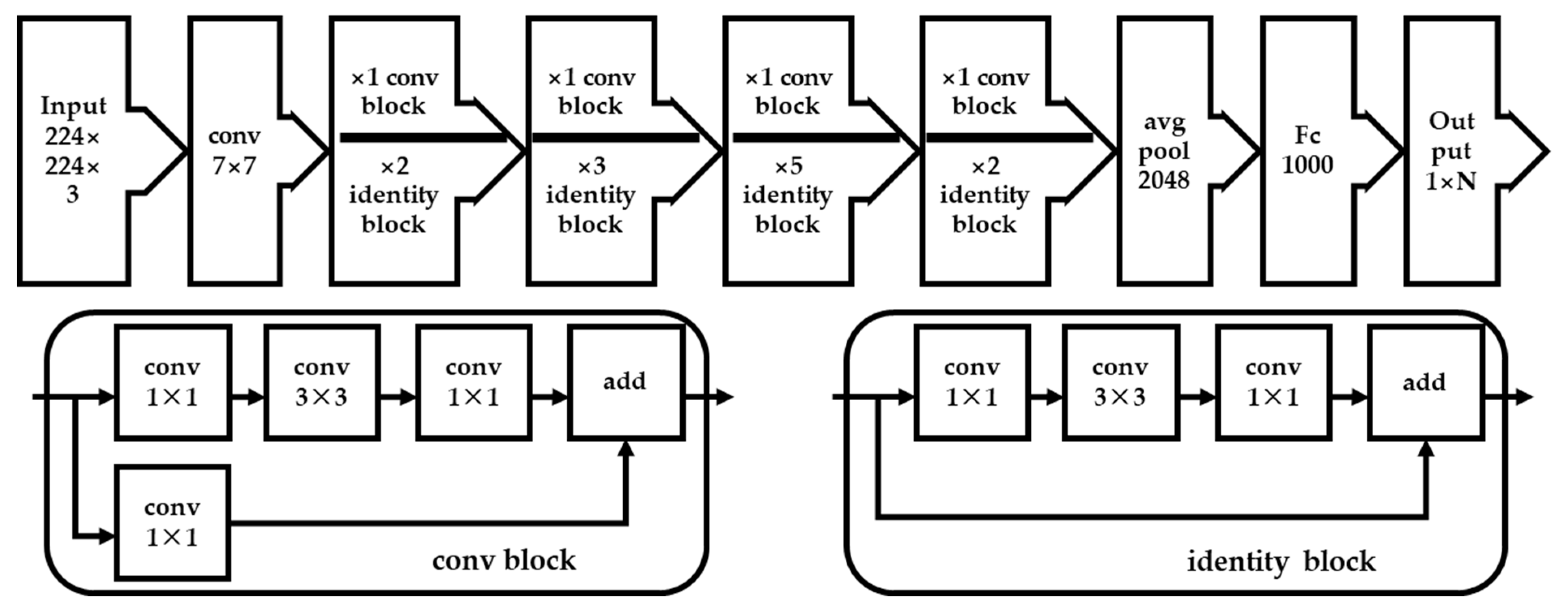
For each residual function F, a bottleneck was designed by using a stack of three layers. To reduce the input/output dimensions, the connected 1 × 1, 3 × 3, and 1 × 1 layers are responsible for reducing, increasing, and restoring the dimensions, respectively.

2.7. DCT

The DCT, first proposed by Nasir Ahmed in 1972, is a widely used transformation technique in signal processing and data compression. A DCT is a Fourier-related transform similar to the discrete Fourier transform (DFT). It transforms a signal or image from the spatial domain to the frequency domain, but only with real numbers.

In the 1D case, the forward cosine transform for a signal g(u) of length M is defined as:

$$G\left(m\right)=\sqrt{\frac{1}{2}}{{\displaystyle \sum }}_{u=0}^{M-1}g\left(u\right)c_m\cos \left(\pi \frac{m\left(2u+1\right)}{2M}\right)$$

(24)

For 0 ≤ m < M, and the inverse transform is:

$$g\left(u\right)=\sqrt{\frac{2}{M}}{{\displaystyle \sum }}_{m=0}^{M-1}G\left(m\right)c_m\cos \left(\pi \frac{m\left(2u+1\right)}{2M}\right)$$

(25)

For 0 ≤ u < M, with:

$$c_m=\{\begin{array}{cc}\frac{1}{\sqrt{2}}& for m=0,\\ 1& otherwise.\end{array}$$

(26)

The index variables (u, m) are used differently in the forward and inverse transforms. DCT is akin to the fast Fourier transform (FFT) but can approximate lines well with fewer coefficients [46]. The 2D DCT transform is equivalent to applying a 1D DCT vertically, then performing a 1D DCT horizontally based on the vertical DCT above.

3. Materials and Methods

3.1. Shallow Feature Fusion-Based Method

3.1.1. HSV Feature

Relative to saturation and brightness value, the hue can show more robust stability, so the number of its bins is set larger than the others. The H, S, and V color channels are uniformly quantized into eight, four, and four bins, respectively, so that in total, 8 × 4 × 4 = 128 color combinations are obtained. The quantized HSV image Hq(x, y) index belongs to [0, 127].

$$F_{HSV}=Histogram\left(H_q\left(x,y\right)\right)$$

(27)

3.1.2. Quantized LBP-SVD Feature

The quantized LBP returns a three-dimensional array containing one histogram of quantized LBP features per cell. The third dimension is the number of uniform LBP patterns. We can apply SVD to each cell to reduce the dimension of the feature size, then extract the first/maximum singular value or L2-norm of singular values.

$$F_{LBP}=MAX\left({\delta }_i\right),{\delta }_i\in {\sum }_{ii}$$

(28)

$$F_{LBP}=\sqrt{{{\displaystyle \sum }}_{i=1}^n{\delta }_i^2},{\delta }_i\in {\sum }_{ii}$$

(29)

The 58-d LBP features are obtained after the above processing.

3.1.3. DTCWT Feature

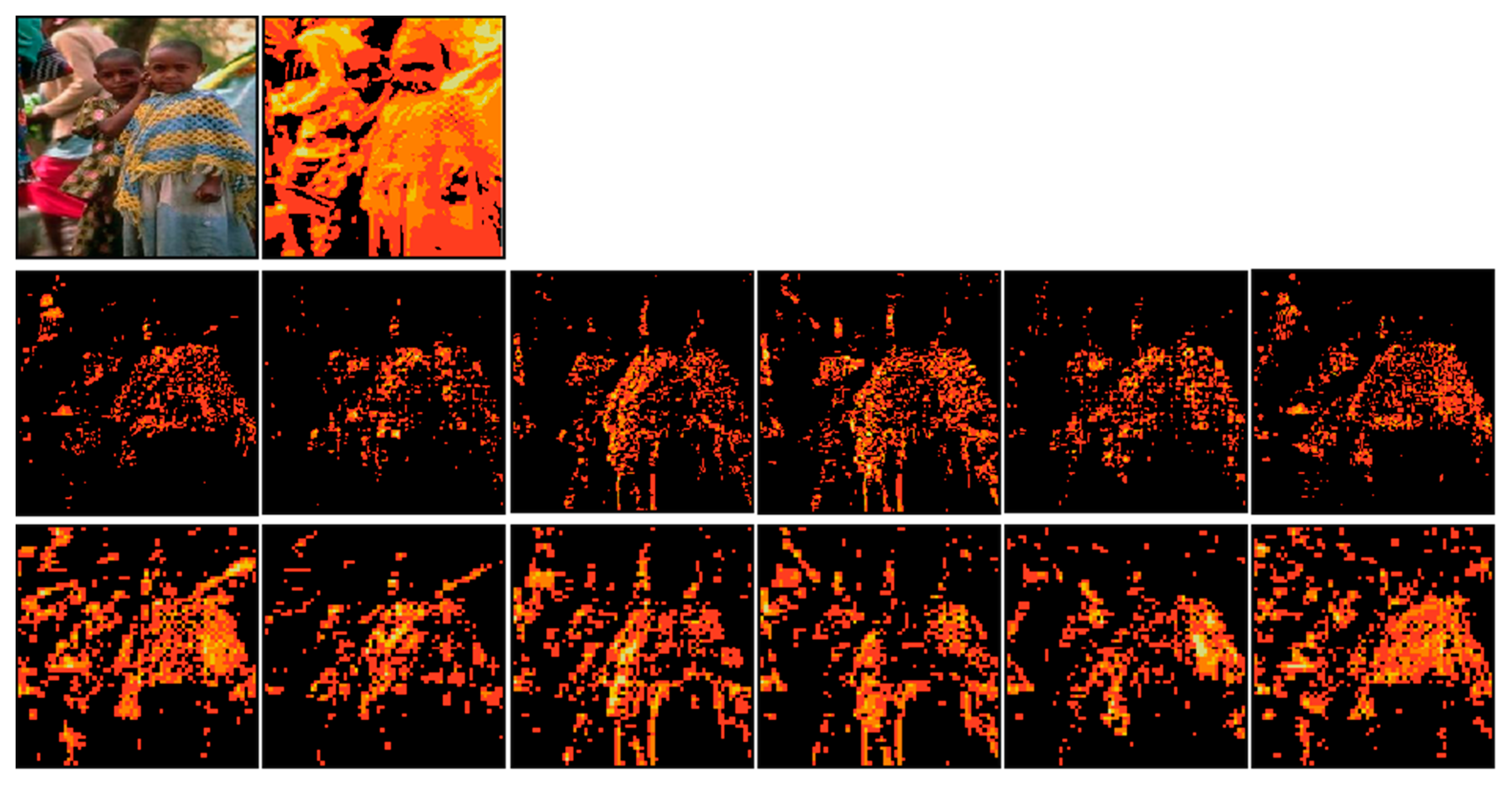
The original feature extraction from DTCWT is based on statistical features such as variance and average for wavelet coefficients of each scale. We are using the “near_sym_b” near-symmetric filters for level−one transform and the “qshift_b” quarter-shift filters for level ≥ two transforms. If it performs a two-level transform, it will return a real lowpass image from the final level and contains the six complex high-pass sub-images for each level, as shown in Figure 1.

Then we use four different statistical features at each sub-image:

$$F_{DTCWT}=\left\{MEA{N}_{coeff},S{D}_{coeff},MEA{N}_{svd}\right\}$$

(30)

Here, SD refers to the standard deviation. Thus, the dimension of DTCWT features is (1 + 2 × 6) = 52.

3.1.4. Shallow Feature Fusion

These three shallow feature vectors are fused as:

$$F_s=\left\{{\Vert F_{HSV}\Vert }_2\times w_1,{\Vert F_{LBP}\Vert }_2\times w_2,{\Vert F_{DTCWT}\Vert }_2\times w_3\right\}$$

(31)

The L2-norm normalizes each type of feature vector. Their weight is generally set to one. It can also be adjusted according to their performance with the iterative method. The fused features lead to a 238-dimensional vector.

3.1.5. Why We Choose Them?

Since the R, G, and B components of the object color in the digital image are all related to the amount of light irradiated on the object, it is difficult to distinguish the object based on these components. HSV is more robust towards external lighting changes. In cases of minor changes in external lighting, hue values vary relatively less than RGB values. XYZ and YUV are computationally less expensive to reach from RGB and less “good” than HSV, HSL, or CIELAB. The CIELAB color space was found to perform at least as well as or better than the other color spaces when measuring image similarity [47]. The HSV color model is more correlated to how humans see colored objects than RGB [42].

LBP has become one of the most prominent texture features, and many new variants have been proposed one after another. The advantages of LBP include avoiding the time-consuming discrete vocabulary pretraining phase in the BoW framework, its overall computational simplicity, and ease of implementation [48]. In addition, uniform patterns make using LBP computationally more efficient without compromising its accuracy. Uniform LBPs can also be applied to obtain rotation invariance [43].

The shape feature reflects the spatial position relationship between the features, and it is more likely to contribute to human visual sensitivity than the color feature and texture feature. Considering the limitations of image retrieval applications based on shape features, we use another texture feature, DTCWT, as an alternative. The effectiveness of this method has also been well verified in previous work [49].

Image local features play a key role in image retrieval. Different kinds of local descriptors represent other visual contents in an image. The local descriptors (SIFT, SURF, and HOG) maintain invariance to rotation, scale scaling, and brightness variation and holds a certain degree of stability against viewing angle changes, affine transformation, and noise [50]. However, it is impossible to extract these features for smooth-edged targets accurately [51], and their real-time performance is not high [52]. Therefore, the image representation methods (BoW, Fisher Vector (FV), VLAD model, etc.) aggregate local image descriptors by treating image features as words and ignoring the patches’ spatial relationships.

The handcrafted local descriptors dominated many domains of computer vision until the year 2012, when deep CNN achieved record-breaking image classification accuracy. Therefore, these local features are skipped in this paper, and only shallow features and depth features are used for image retrieval performance analysis.

3.2. Deep Feature Fusion-Based Method

3.2.1. Place-Centric Networks

How to assign a semantic category to an image based on the visual content of the image (for example, classroom, street, etc.) is the goal of image scene classification, and it is also the basis for problems such as image retrieval, image content analysis, and target recognition. We can combine scene semantics with object content and use multimodal information to enhance image retrieval performance. The research has studied that using place features has good performance for scene classification [53].

In our previous research [54], we studied recognizing the scene type of a picture by using a neural network to train the images in the scene category. The place datasets we used are mainly taken from the Places database [53]. Some existing categories have been merged based on this data set, and some new types have been added. The final number of categories is 434. Considering the performance, parameters, and computing complexity, we used the pre-trained GoogleNet and ResNet−50 support packages from the MATLAB Neural Network Toolbox [55] to train the Place dataset. We took about 540 images (500 normal images and 40 cartoon images) from each category for the training set. We used 60 images (50 normal images and 10 cartoon images) for the validation set with 100 images (80 normal images and 20 cartoon images) for the test set. The training dataset is much smaller than those in Places365, and the training iteration is also not large enough. The accuracy values of classification are lower than those in the Places365 dataset.

3.2.2. Deep Feature Extraction

Generally, the fully connected layers are directly extracted as the CNN features by the pre-trained model. However, some researchers have found that the middle layer is more suitable for object retrieval. In the present paper, we use the output vectors of the average pooling layer instead of Fc layers as the inputs of the DCT transform. A diagram of deep feature extraction is shown in Figure 2.

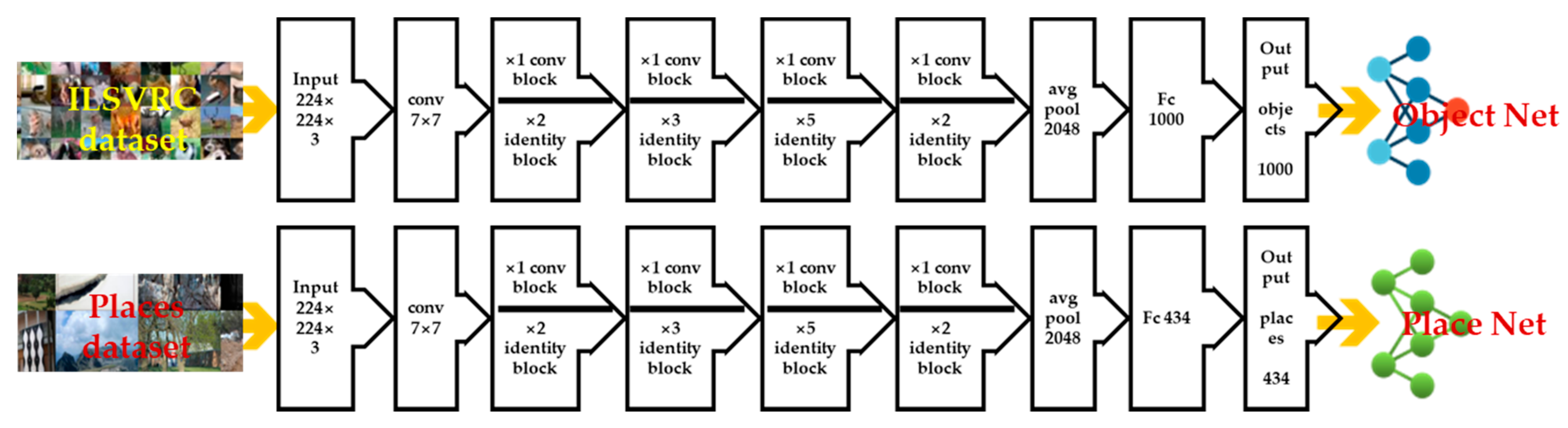
The pre-trained models are generated by using the same ResNet50 network to train different data sets. As shown in Figure 3, the object-centric image dataset ILSVRC and place-centric image dataset Places are used for training, respectively.

3.2.3. Deep Feature Fusion

Through the above-mentioned deep feature extraction method, the pre-trained ResNet50 and PlaceNet networks are used to extract the object-centric and scene-centric features of the input image. The two types of deep features are fused as:

$$F_D=\left\{F_{object}\times w_1,F_{place}\times w_2\right\}$$

(32)

3.3. Proposed Image Retrieval System

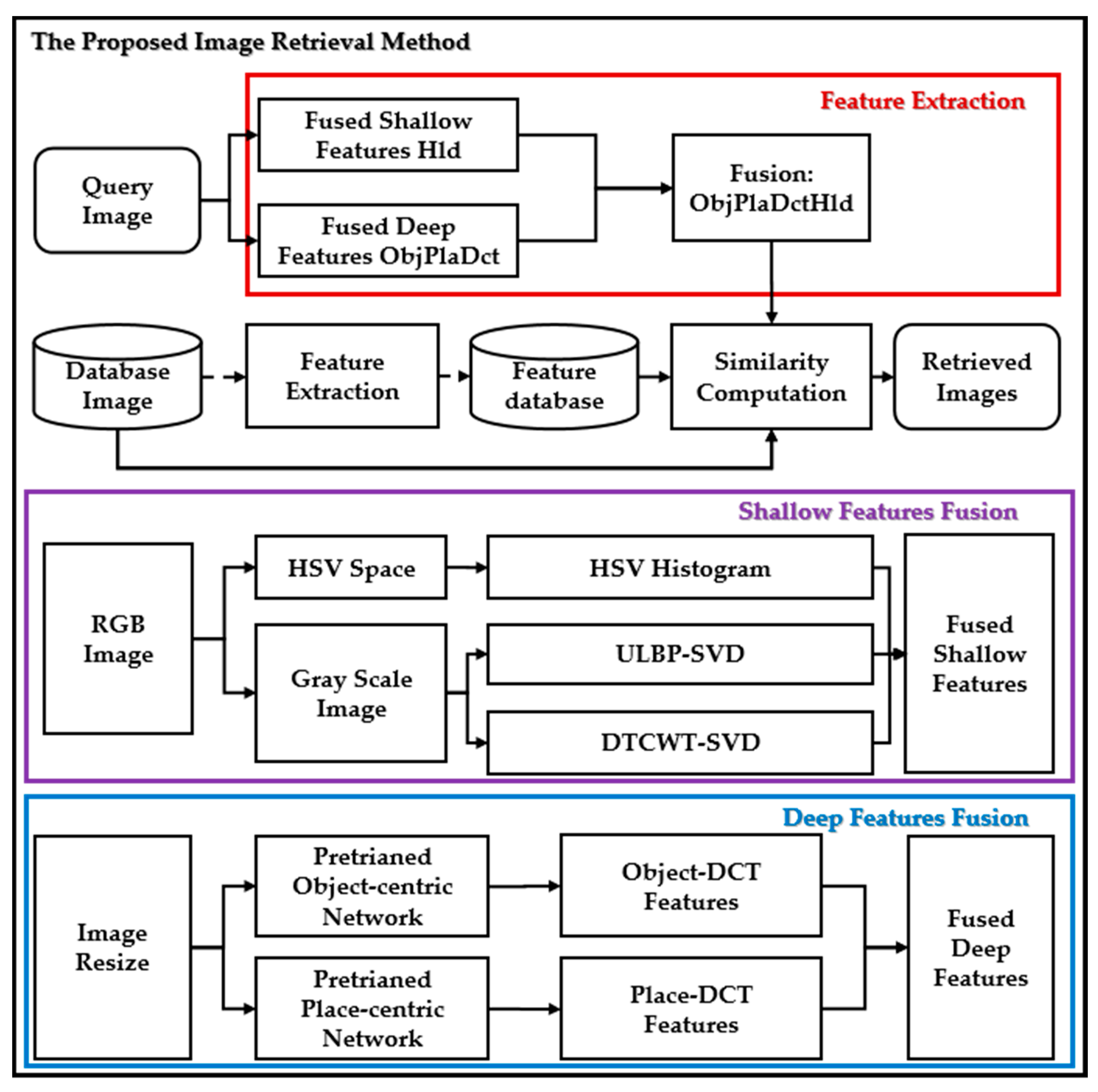
The image retrieval system uses image preprocessing, extracts shallow and deep features from the image, and then calculates the similarity to retrieve the image. Figure 4 shows the proposed image retrieval framework.

• Unlike the method that replaces the original image with DCT coefficients for CNN training [56], this paper uses DCT transform to reduce the features of the Average Pooling layer of CNN features.
• In addition to using ObjCnn features generated by object recognition, this method also combines PlaCnn features generated by scene recognition to generate fused deep features.
• This method also uses global shallow features and uses SVD to reduce the dimensionality of ULBP and DTCWT.
• Weights respectively combine the shallow features, the deep features, the shallow features, and the deep features.

4. Experimental Results and Analyses

4.1. Evaluation Methods

4.1.1. Similarity Measure

Let p = (p₁, p₂, …, p_n) and q = (q₁, q₂, …, q_n) are two n-dimensional real vectors. The following function can measure the similarity between them.

Cosine similarity [57] is a commonly used similarity measure for real-valued vectors. The cosine of two non-zero vectors can be derived by using the Euclidean dot product formula:

$$p·q=\Vert p\Vert ·\Vert q\Vert \cos \theta$$

(33)

Given two vectors of attributes, the similarity cos(θ) is represented using a dot product and magnitude as:

$$sim\left(p,q\right)=\cos \left(\theta \right)=\frac{p·q}{\Vert p\Vert \Vert q\Vert }=\frac{{\sum }_{i=1}^n{p}_i{q}_i}{\sqrt{{\sum }_{i=1}^n{p}_i^2}\sqrt{{\sum }_{i=1}^n{q}_i^2}}$$

(34)

where p_i and q_i are components of vectors p and q, respectively.

The Euclidean distance (L2 distance) is the most obvious way of representing the distance between two points. The Euclidean distance between two points p and q is given by [58]:

$$d\left(p,q\right)=\sqrt{{\left(p_1-q_1\right)}^2+{\left(p_2-q_2\right)}^2+\cdots +{\left(p_n-q_n\right)}^2}$$

(35)

The Manhattan distance (L1 distance) [59] is a metric in which the distance between two points is the sum of the absolute differences of their Cartesian coordinates. For example, the Manhattan distance d₁ between two vectors p, q is the sum of the lengths of the projections of the line segment between the points onto the coordinate axes.

$$d_1\left(p,q\right)={\Vert p-q\Vert }_1={{\displaystyle \sum }}_{i=1}^n\left|p_i-q_i\right|$$

(36)

The Minkowski distance [60] is a metric in a normed vector space that can be considered a generalization of both the Euclidean distance and the Manhattan distance. The Minkowski distance of order k between two vectors p and q is defined as:

$$d\left(p,q\right)={\left({{\displaystyle \sum }}_{i=1}^n{\left|p_i-q_i\right|}^k\right)}^{\frac{1}{k}}$$

(37)

The Canberra distance [61] is a weighted version of the Manhattan distance. The Canberra distance d between vectors p and q in an n-dimensional real vector space is given as follows:

$$d\left(p,q\right)={{\displaystyle \sum }}_{i=1}^n\frac{\left|p_i-q_i\right|}{\left|p_i\right|+\left|q_i\right|}$$

(38)

4.1.2. Precision and Recall

Precision and Recall [62] are used to evaluate the performance of the proposed method. Both are therefore based on relevance. The precision (P) of the kth image is equivalent to the ratio of relevant images retrieved (N_TP) to the total number of images retrieved (N_TR):

$$P\left(I_k\right)=\frac{N_{TP}}{N_{TR}}\times 100\%$$

(39)

Recall (R) is the ratio of relevant images retrieved (N_TR) to the number of relevant images in the database (N_RI):

$$R\left(I_k\right)=\frac{N_{TP}}{N_{RI}}\times 100\%$$

(40)

The average precision (AP)/average Recall (AR) is obtained by taking the mean over the precision/recall values at each relevant image:

$$AP=\frac{1}{N_Q}{{\displaystyle \sum }}_{k=1}^{N_Q}P\left(I_k\right)$$

(41)

$$AR=\frac{1}{N_Q}{{\displaystyle \sum }}_{k=1}^{N_Q}R\left(I_k\right)$$

(42)

where N_Q is the number of queries and I_k represents the kth image in the database.

The rank-based retrieval system displays the appropriate set of the top k retrieved images. The P and R values of each group are displayed graphically with curves. The curves show the trade-off between P and R at different thresholds.

4.2. Experimental Results

We conducted experiments on three commonly used datasets, namely, Corel-1k [63], Corel-5k [64], Corel-DB80 [65], and Oxford Building [66], to analyze the performance of the proposed method. All images in the first three datasets are used as query images, and then the retrieval precision/recall of each image, each category, and the total dataset are computed.

4.2.1. Corel-1k Dataset

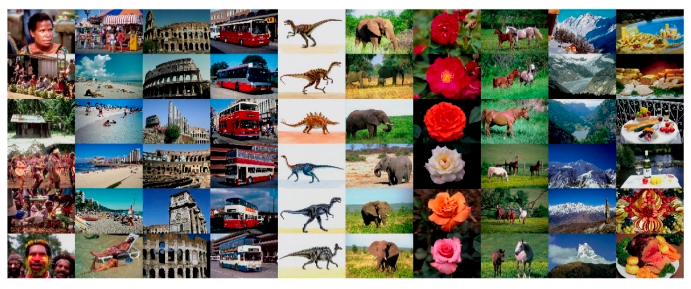
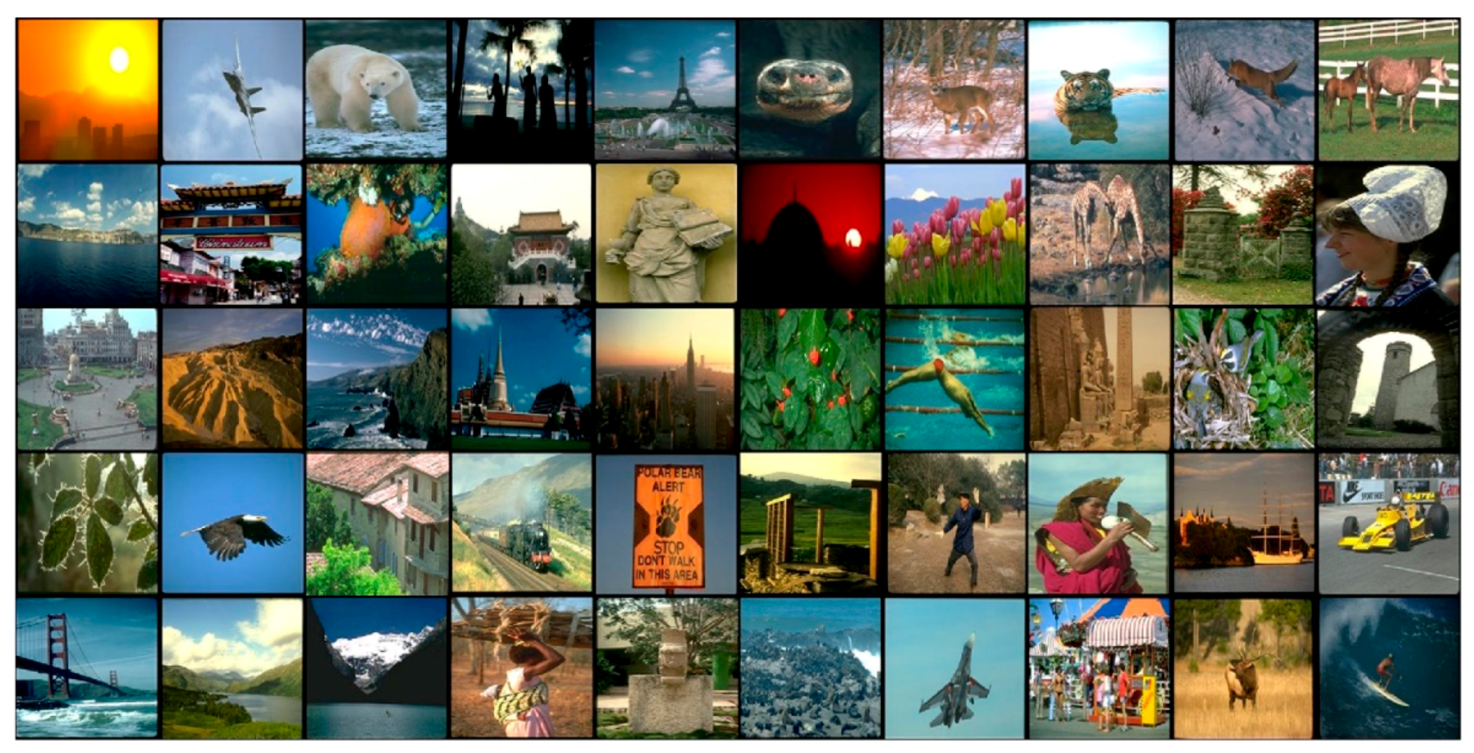
The Corel-1k dataset has ten categories, and each category has 100 images with a resolution of 256 × 384 pixels or 384 × 256 pixels. Six samples of each type are shown in Figure 5.

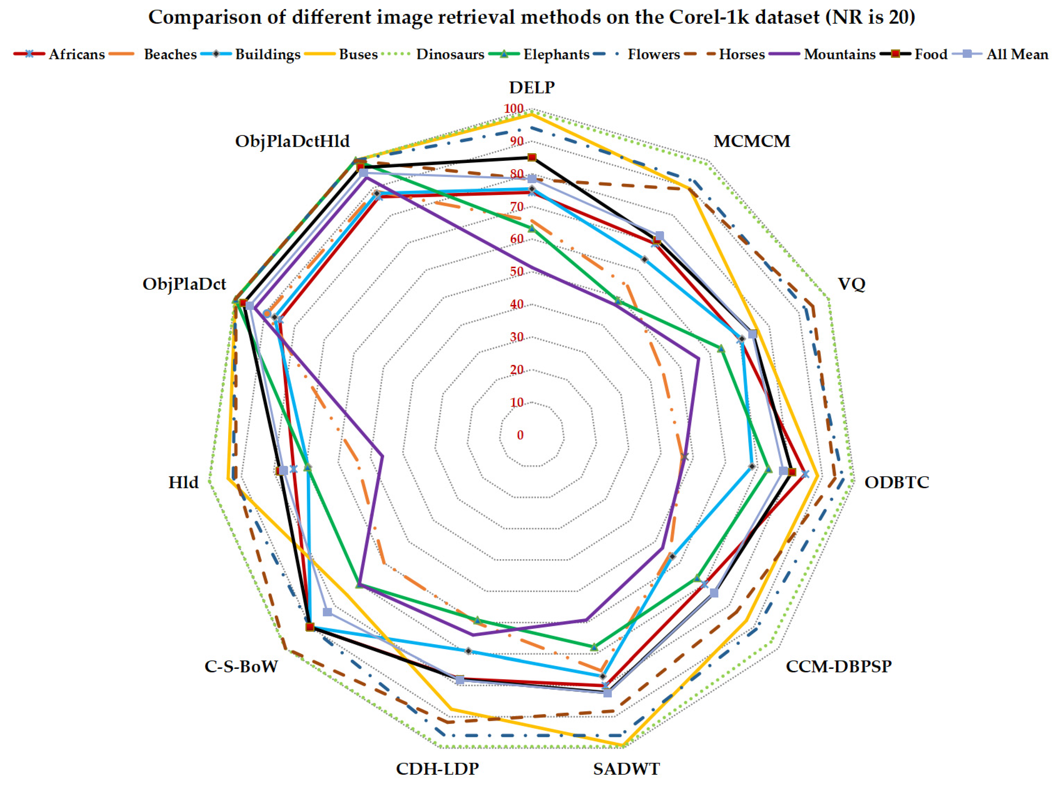
So far, most of the image retrieval research use Corel-1k as the benchmark for image retrieval and classification. However, it lacks a unified performance evaluation standard, and the experimental results are not convenient for later researchers as a reference. Therefore, this paper synthesizes the parameters used in various methods to explain the data to provide convenience for later researchers. Three comparison experiments with different numbers of retrieved (NR) images are considered.

Table 1. Comparison of different image retrieval methods on the Corel-1k dataset (Top NR is 20). The bold values indicate the best results.

Category	Average Precision (%), Top NR = 20
	DELP [10]	MCMCM [6]	VQ [22]	ODBTC [24]	CCM-DBPSP [33]	SADWT [14]	CDH-LDP [33]	C-S-BoW [34]	Hld	ObjPlaDctHld
Africans	74.3	69.7	70.2	84.7	70	80.1	77.9	90	73.7	86.7
Beaches	65.6	54.2	44.4	46.6	56	75.3	60.1	60	54.2	88.8
Buildings	75.4	63.9	70.8	68.2	57	77.1	69.1	90	69.3	88
Buses	98.2	89.6	76.3	88.5	87	99.2	87.6	75	94.1	100
Dinosaurs	99.1	98.7	100	99.2	97	99.5	99.4	100	99.9	100
Elephants	63.3	48.8	63.8	73.3	67	67.8	59.2	70	69.5	100
Flowers	94.1	92.3	92.4	96.4	91	96.0	95.8	90	92.5	100
Horses	78.3	89.4	94.7	93.9	83	88.2	91.8	100	91.7	99.9
Mountains	51.3	47.3	56.2	47.4	53	59.2	64	70	46.3	93.8
Food	85.0	70.9	74.5	80.6	74	82.3	78.1	90	78	97.4
All Mean	78.46	72.5	74.3	77.9	74	82.47	78.31	83	76.9	95.44

lists the APs generated by different methods in each category of the Corel-1k dataset with NR = 20. The methods DELP [10], MCMCM [6], VQ [22], ODBTC [24], CCM-DBPSP [32], CDH-LDP [33], SADWT [14], and C-S-BoW [34] are compared.

The proposed Hld method using fused shallow features has better performance than MCMCM, VQ, and CCM-DBPSP. The ObjPlaDctHld method using combined deep features performed much better than Hld and other compared methods, especially in Beaches, Elephants, Mountains, and Food categories. A radar chart of the compared results is shown in Figure 6.

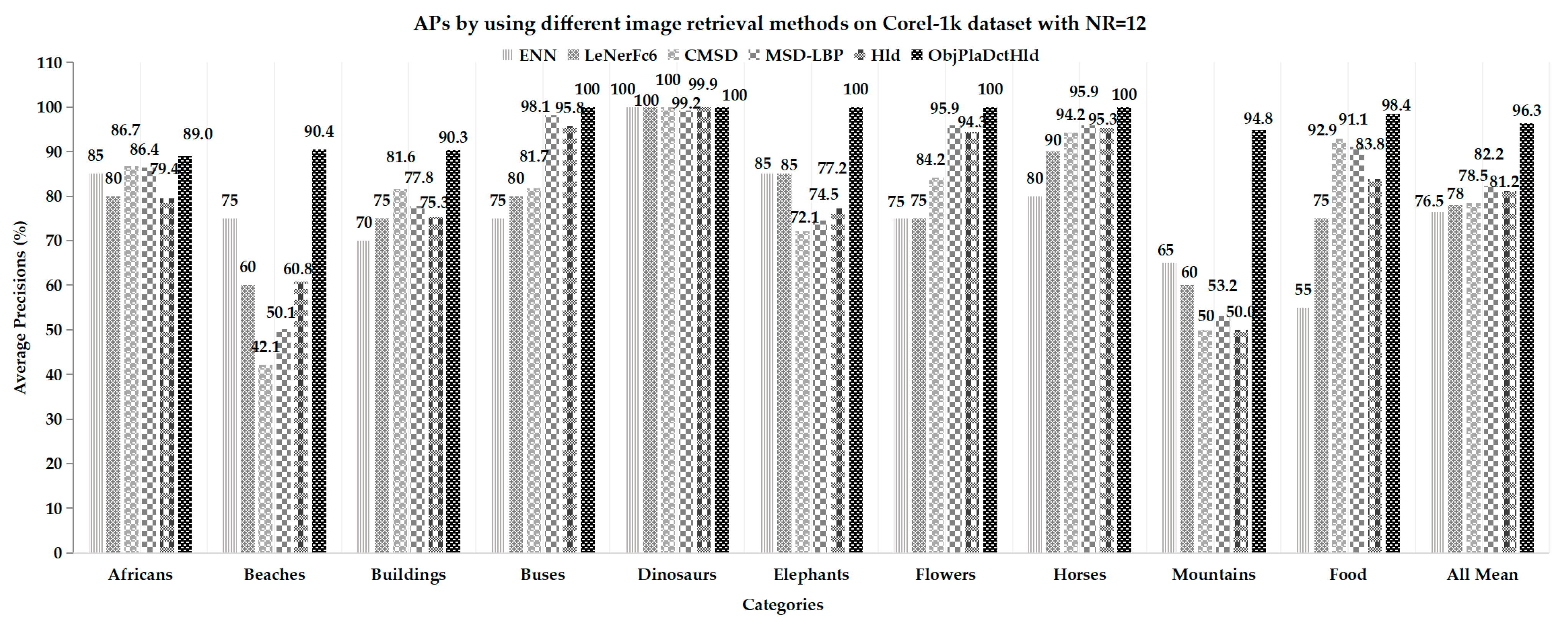
Figure 7 shows the APs of the Corel-1k dataset with the NR = 12. Here, the methods of CMSD [35] and MSD-LBP [36] are based on shallow feature fusion. The methods of ENN [27] and LeNetF6 [28] are based on deep features. The proposed Hld method even showed relatively better performance than ENN, LeNetFc6, and CMSD on average. However, most of them showed worse performance in categories such as Beaches and Mountains. There is a big difference in object detection with these scene places and difficulty using low-level features for classification.

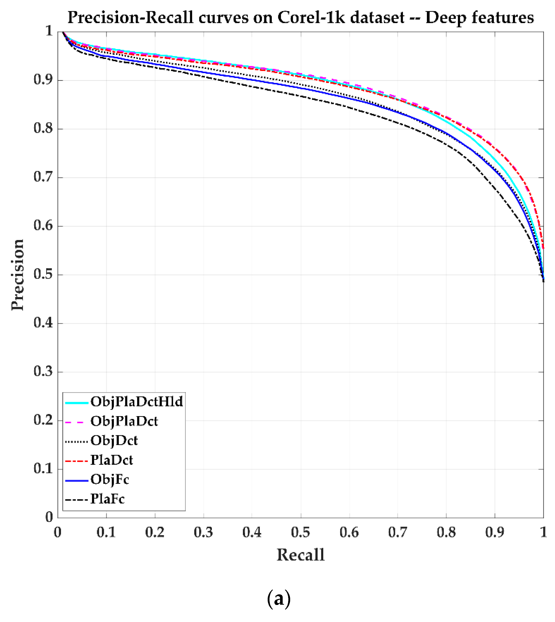
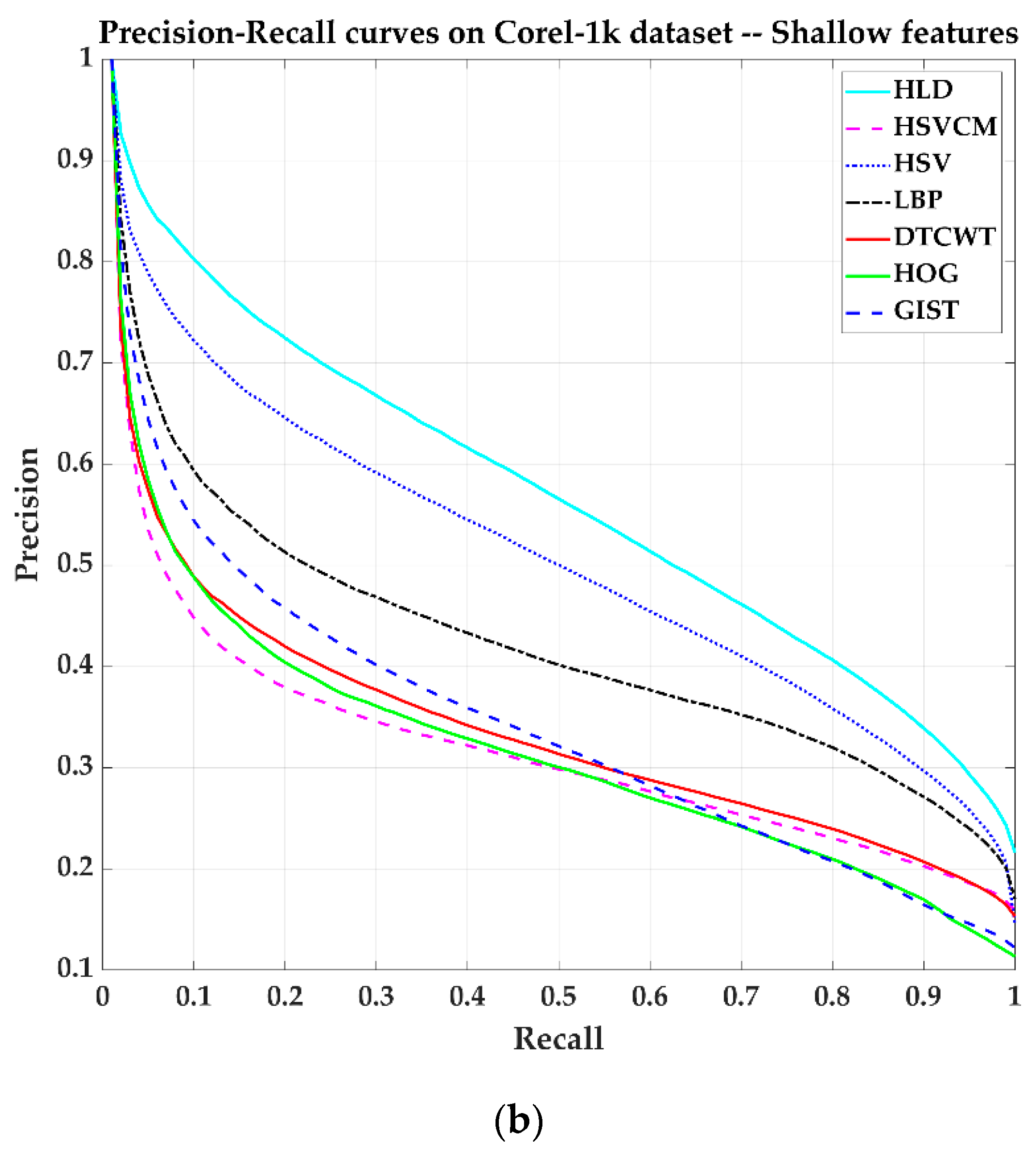
Figure 8 shows image retrieval results on the Corel-1k dataset by some algorithms. The ObjPlaDctHld method has about 0.3 more improvements on average than Hld when Recall = 1. The shallow features fusion method HLD has better performance than those using a single type of feature.

4.2.2. Corel-5k Dataset

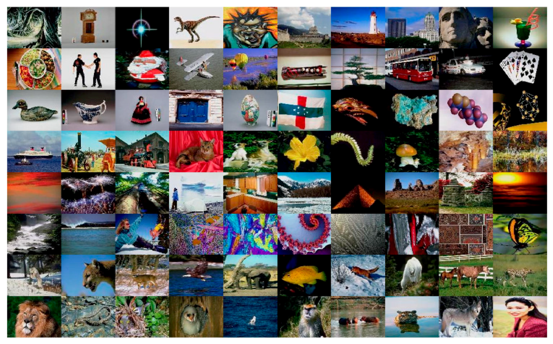
The Corel-5k dataset contains 50 categories. Each category contains 100 192 × 128 or 128 × 192 images in JPEG format. A sample of each category is shown in Figure 9.

Here, we test the performance of the proposed method using different features, the results are listed in

Table 2. APs and ARs results of using different features on Corel-5k dataset (Top NR = 12).

Features	Feature Type	Feature Length	APs (%)	ARs (%)
HSV histogram	Shallow	128	31.27	3.75
HSVCM	Shallow	9	17.72	2.13
Quantized LBP-SVD	Shallow	58	20.74	2.49
DTCWT-SVD	Shallow	52	16.76	2.01
Hld	Shallow-Fusion	238	37.09	4.45
ObjDct	Deep, AVG-DCT	256	49.08	5.89
PlaDct	Deep, AVG-DCT	256	50.63	6.08
ObjFc	Deep, Fc layer	1000	48.19	5.78
PlaFc	Deep, Fc layer	434	47.30	5.68
ObjPlaDct	Deep-Fusion	512	51.63	6.20
ObjPlaDctHld	Deep-Shallow-Fusion	750	54.99	6.60

. The deep features are extracted using ResNet architecture. “DCT” refers to the use of front nth DCT coefficients. “Fc” indicates that the extracted features come from the fully connected layer.

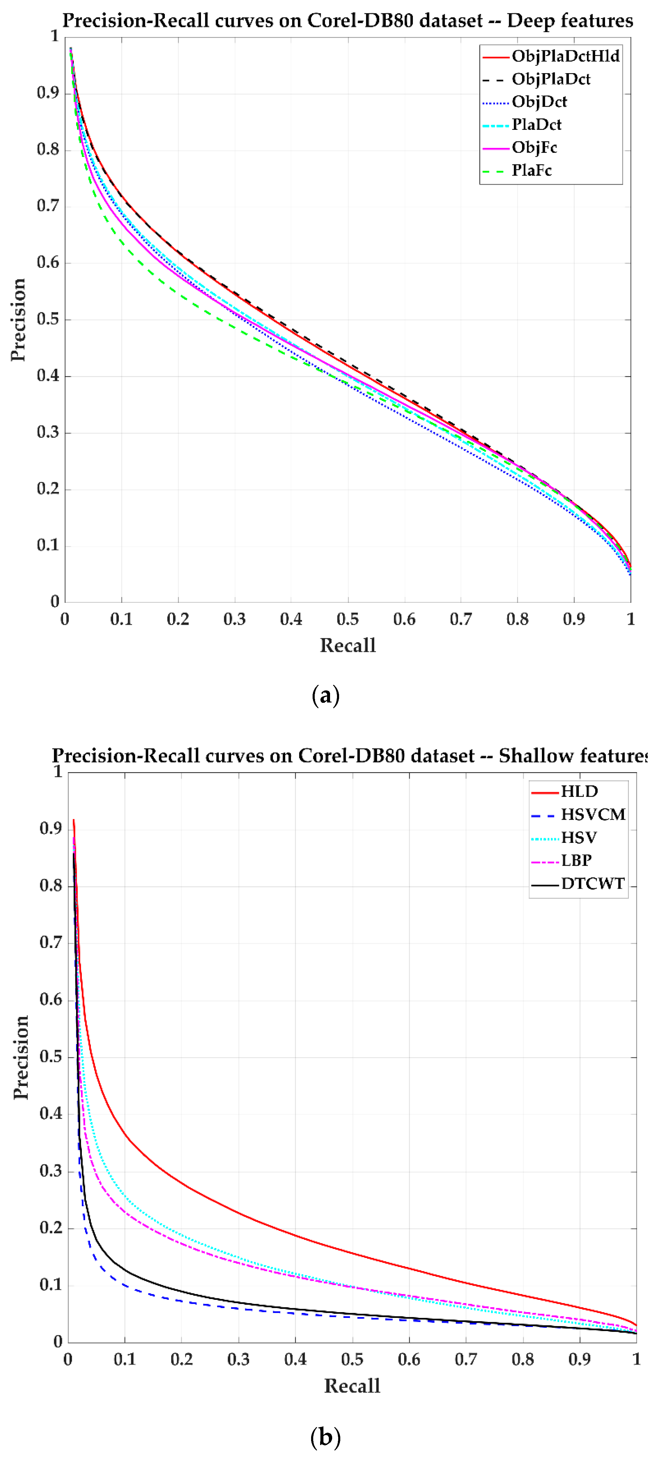
The experimental results show that using deep features for image retrieval is a significant improvement over shallow features. Fusion features also show better performance than individual features. Among these shallow features, the color feature contributes the most to image retrieval.

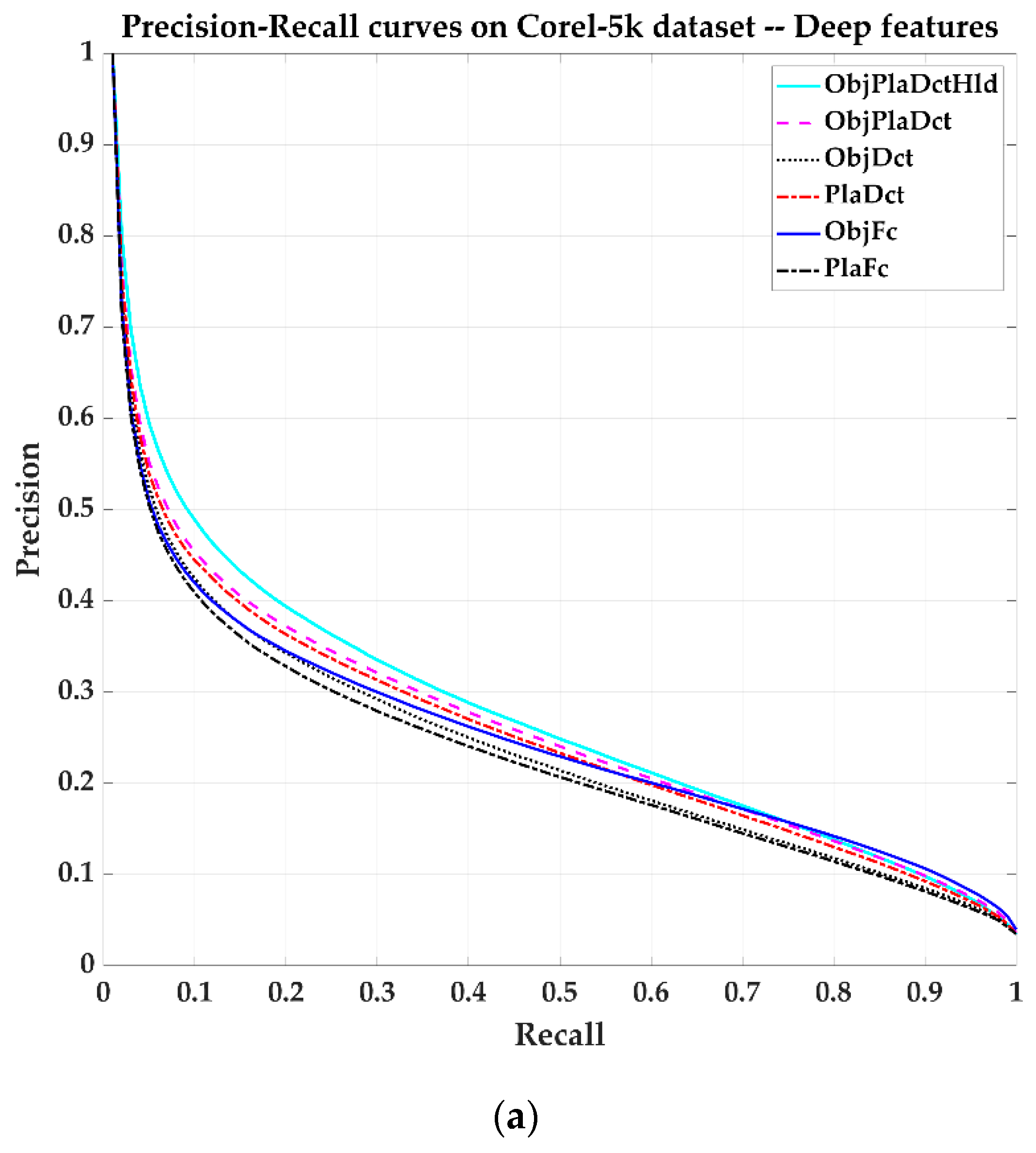
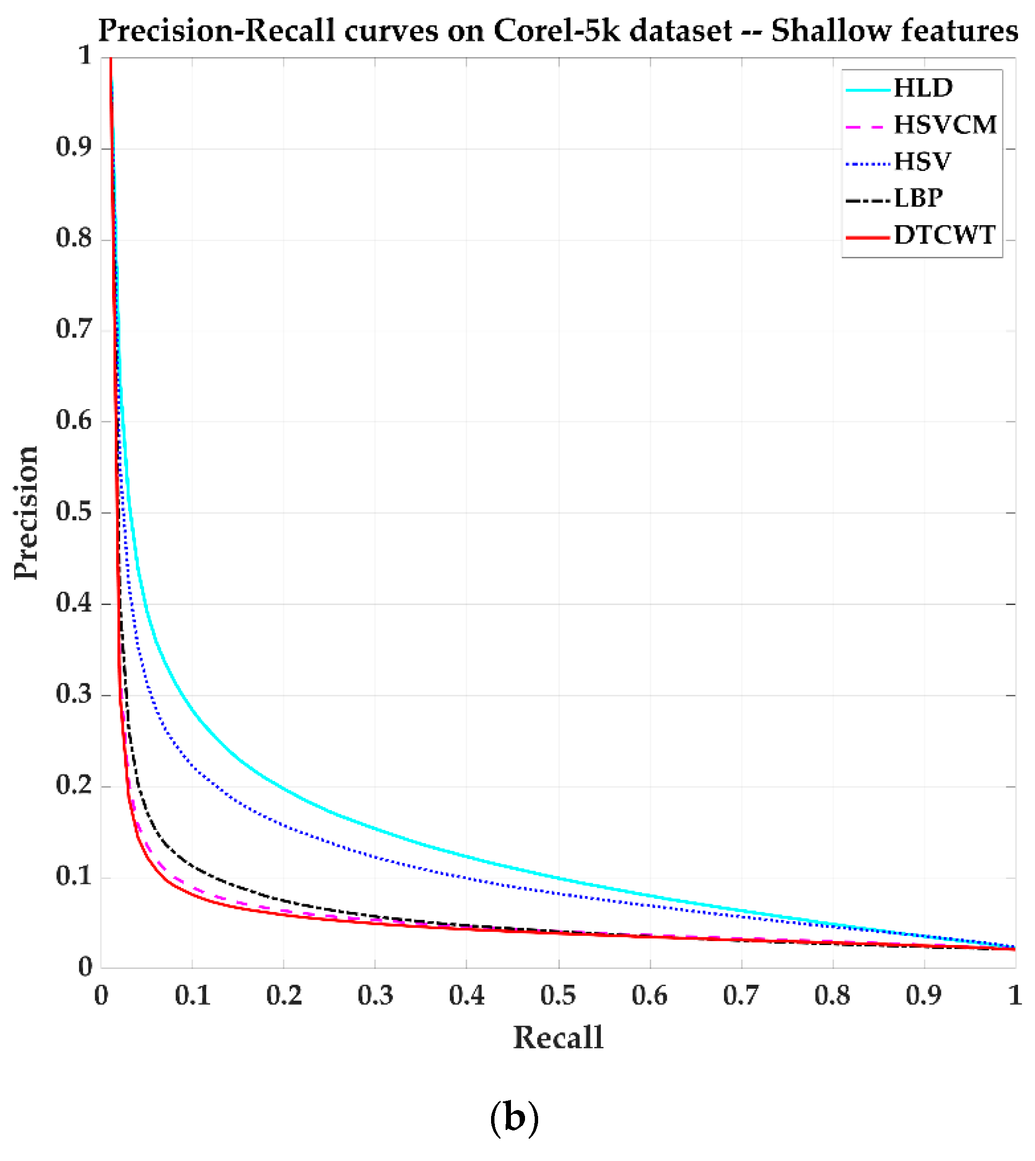
Figure 10 shows Precision-Recall curves corresponding to these methods. Again, the deep feature-based method showed much better performance than the shallow feature-based method.

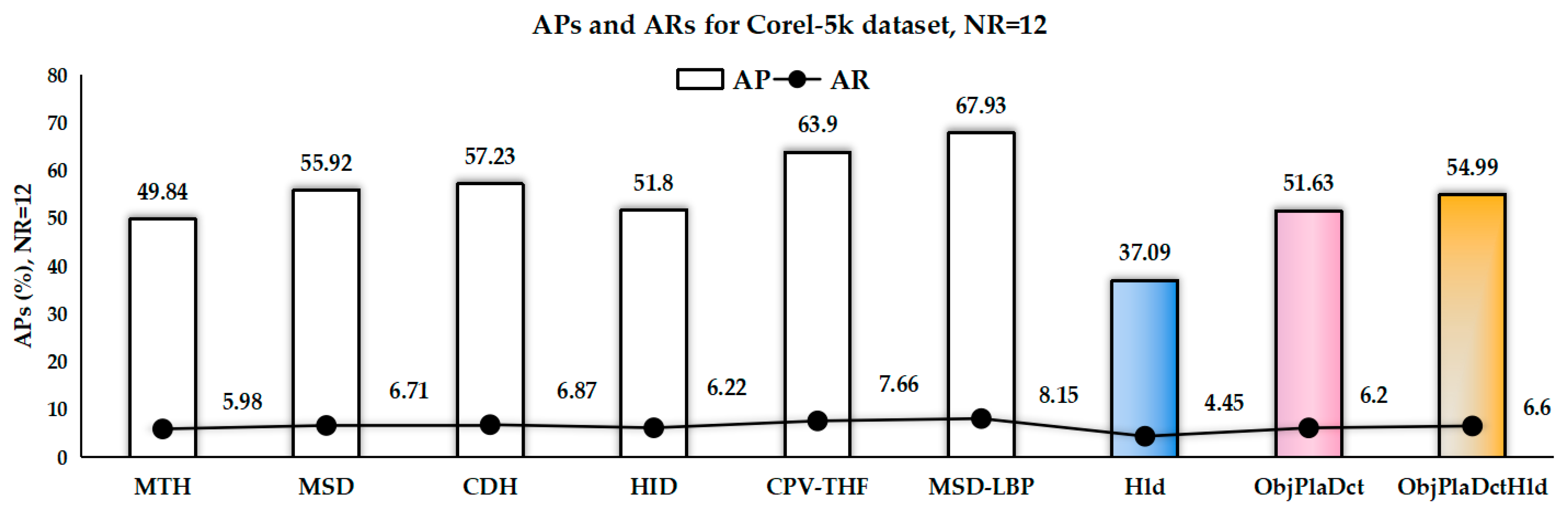
Figure 11 shows the APs and ARs on the Corel-5k dataset of the proposed method compared to methods such as MSD [64], MTH [67], CDH [68], HID [69], CPV-THF [70], MSD-LBP [36]. Unfortunately, the results of our proposed algorithm are not the best. Although our method shows better performance than MSD-LBP on the Corel-1k dataset, it lags far behind on the Corel-5k dataset. This is because the deep features are based on many datasets for pre-network training.

The micro-structure map defined in the MSD method captures the direct relationship between an image’s shape and texture features. MTH integrates the co-occurrence matrix and histogram advantages and can capture the spatial correlation of color and texture orientation. HID can capture the internal correlations of different image feature spaces with image structure and multi-scale analysis. The correlated primary visual texton histogram features (CPV-THF) descriptor can capture the correlations among the texture, color, intensity, and local spatial structure information of an image.

4.2.3. Corel-DB80 Dataset

A dataset with 80 concept groups, which contains 10,800 images, is manually divided. Each category contains almost more than 100 120 × 80 or 80 × 120 images in JPG format. One sample from each category is shown in Figure 12.

Figure 13 shows the AP-AR curves corresponding to some methods. The DCT-based method still performed better than using the fully connected layer. The deep feature-based method was much better than the shallow feature-based method. The slope of the resulting curve based on the deep feature is relatively flat. In this experiment, the ObjPlaDctHld method fused with shallow features slightly improves the performance compared to only using the ObjPlaDct method when Recall is not high enough. When Recall is 0.5, the AP drops to 0.48, much higher than that in the Corel-5k dataset (where AP is 0.25). The difference in the APs of the two datasets illustrates the impact of accurate annotation of the data set on the experimental results.

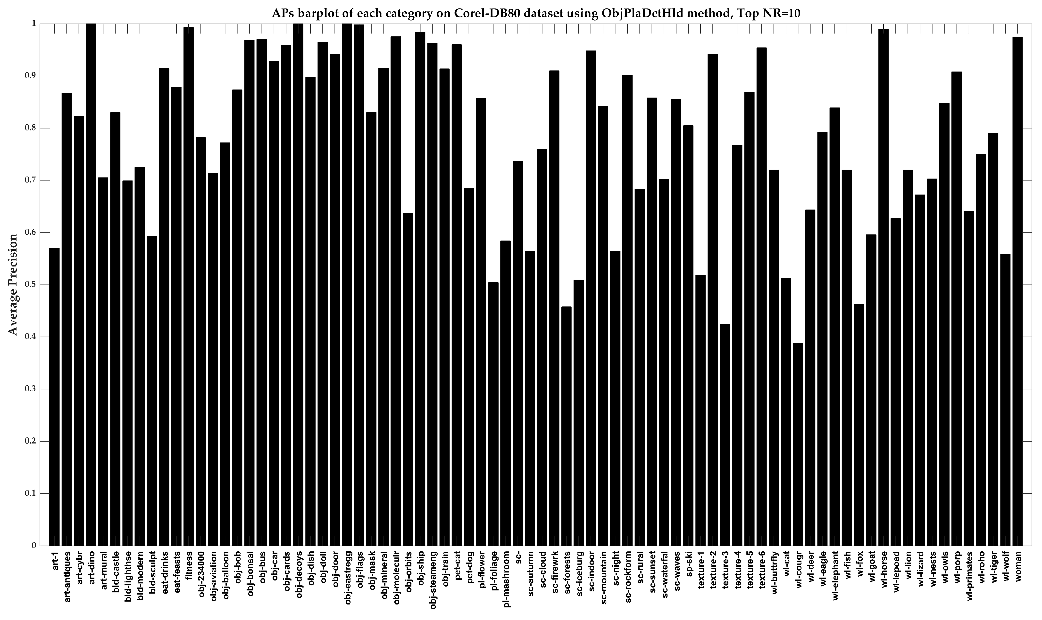
Figure 14 shows the AP of each category with Top NR = 10. The proposed method also has its shortcomings when dealing with categories such as art, buildings, scenes, and wildlife. Nevertheless, it can identify and retrieve most categories.

4.2.4. Oxford building Dataset

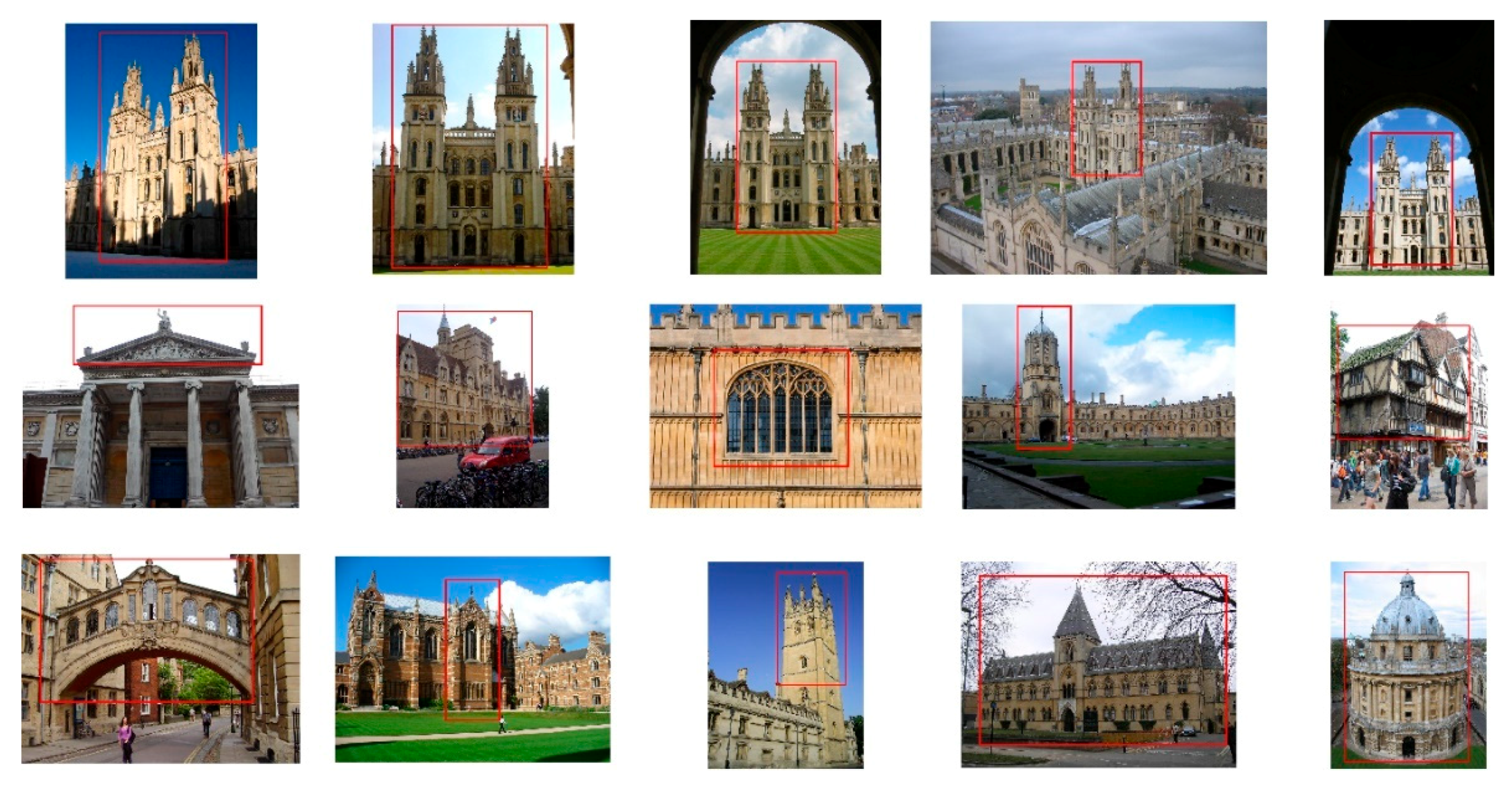
We continue to evaluate the proposed method on Oxford Buildings dataset. The Oxford Buildings dataset contains 5063 images downloaded from Flickr by searching for particular landmarks. For each image and landmark in the dataset, four possible labels (Good, OK, Bad, Junk) were generated. The dataset gives a set of 55 queries for evaluation. The collection is manually annotated to create comprehensive ground truth for 11 different landmarks, each represented by five possible queries. The mean average precision (mAP) [71] is used to measure the retrieval performance over the 55 queries. In the experiment, each image is resized to the shape of 224 × 224. Some typical images of the dataset are shown in Figure 15.

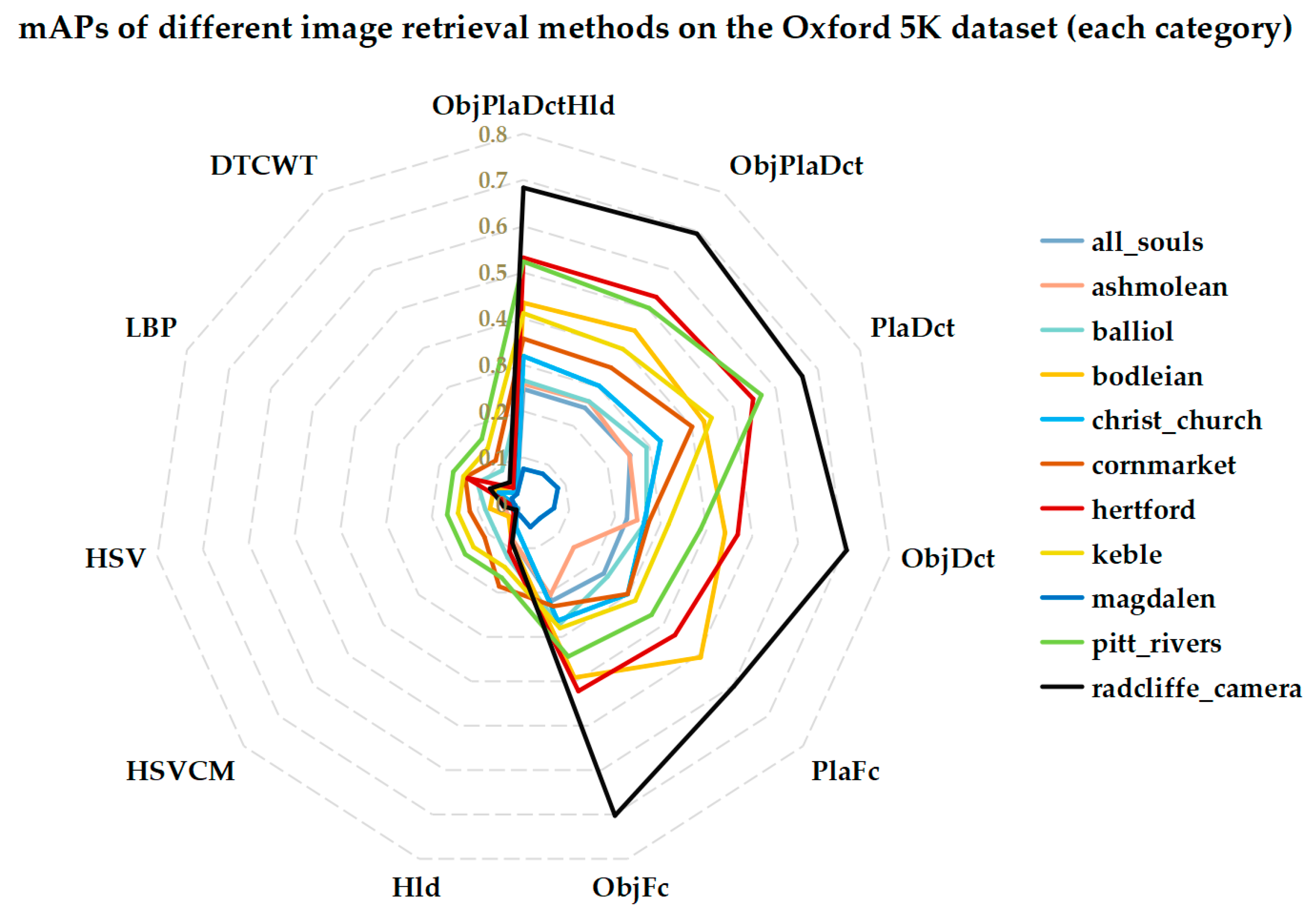
A radar chart of the compared results on each category is shown in Figure 16. The results show that the mAP based on shallow features is significantly lower than the mAP based on the in-depth part. The maximum value is obtained on the ‘RadCliffe_camera’ class, but only slightly greater than 0.7, the minimum value is received at the ‘Magdalen’ category, and the value is not more than 0.1. The fused deep feature did not significantly improve the retrieval results as a whole, and when the weight of each part is the same, the results will even decrease. Given that the performance of the shallow feature is deficient in the landmark categories, the performance of the ObjPlaDctHld is not excellent. Akin to the test results on the previous dataset, the DCT-based method still performed better than using the fully connected layer.

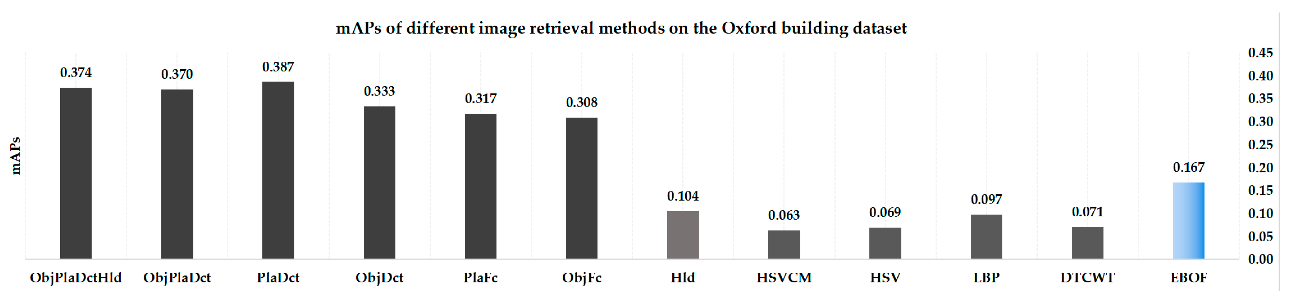
Figure 17 shows the mAP of the total dataset using different image retrieval methods. Here, we use the extended bag-of-features (EBOF) [72] method as the compared method. Its codebook size is K = 1000. The performance of the EBOF method is much better than that using shallow features and is much lower than that using the deep features-based method. For the Oxford 5K dataset, the PlaDct method based on places-centric features has the best performance.

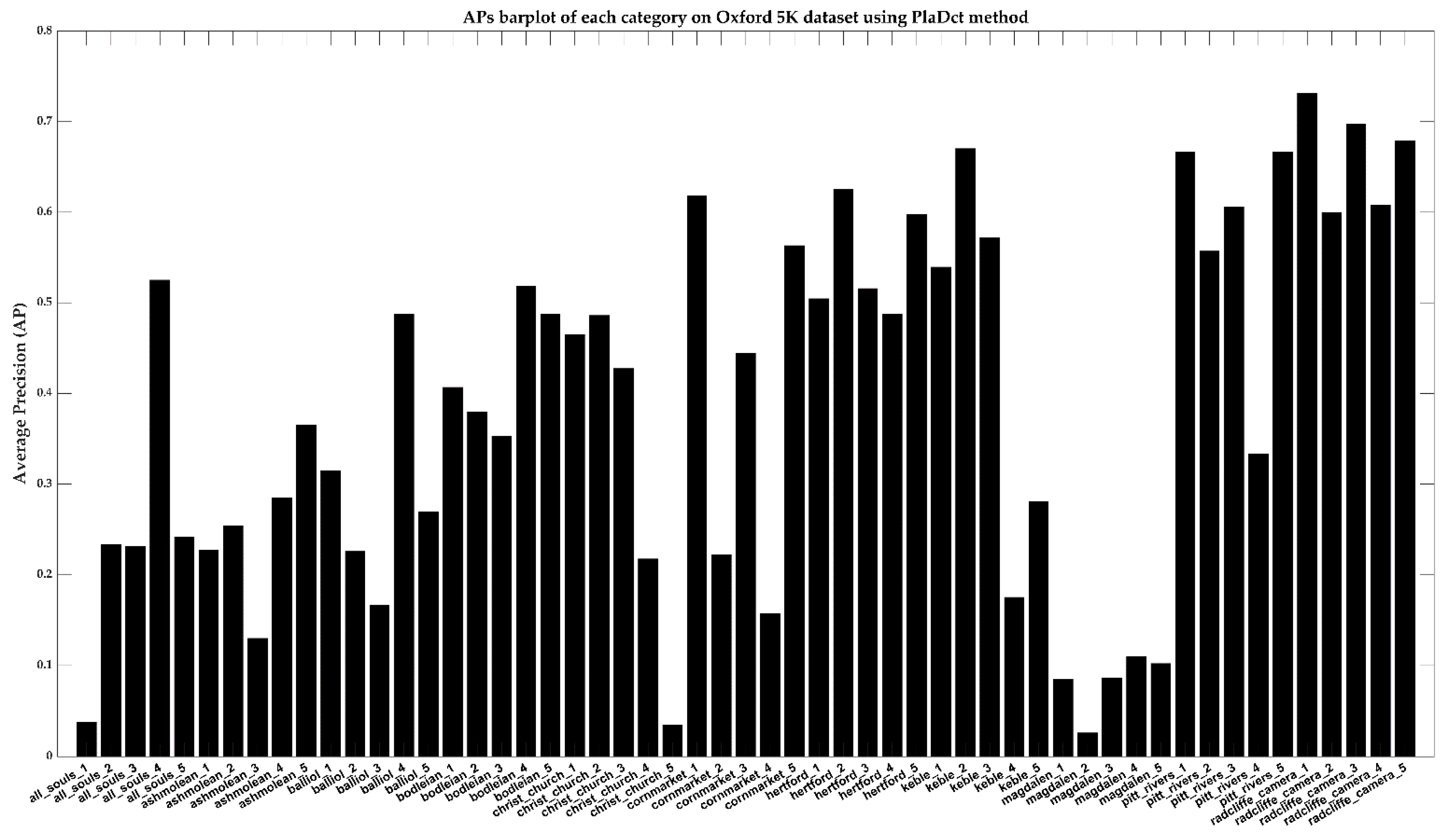
Figure 18 shows the APs of each query using the PlaDct method. Retrieving results on several categories such as ‘All Souls’, ‘Ashmolean’, and ‘Magdalen’ is not ideal, especially in the ‘Magdalen’ category.

4.3. Influence of Variable Factors on the Experiment

4.3.1. Similarity Metrics

Here, we conduct comparative experiments on the dataset by using different similarity metrics.

Table 3. APs and ARs results using different methods with different distance or similarity metrics, Top NR = 20.

Method	Dataset	Performance	Distance or Similarity Metrics
			Canberra	Weighted L1	Manhattan	Cosine Correlation
ResNetFc	Corel-1k	AP (%)	94.09	93.87	93.99	94.47
		AR (%)	18.82	18.77	18.80	18.89
	Corel-5k	AP (%)	42.30	42.35	42.36	42.72
		AR (%)	8.46	8.47	8.47	8.54
Hld	Corel-1k	AP (%)	76.28	76.91	76.59	66.24
		AR (%)	15.26	15.38	15.32	13.25
	Corel-5k	AP (%)	30.40	30.94	30.54	23.85
		AR (%)	6.08	6.19	6.11	4.77

lists the APs and ARs by the proposed methods with different distance or similarity metrics. The Top NR is 20. The deep feature ResNetFc extracted from the ResNet50 fully connected layer and fused shallow features Hld are used for the test.

Here, in the weighted L1 metric, 1/(1 + p_i + q_i) is the weight, as shown in Table 3. When different methods are used, the best similarity metric changes. The Canberra metric appears to be more stable.

4.3.2. CNN Architecture

Here, we conduct comparative experiments on the dataset by using different CNN architectures. The deep features are extracted in the Fc layer. AlexNet, ResNet50, GoogleNet, GooglePlaces, and ResPlaces are used for comparison experiments. GooglePlaces and ResPlaces are pre-trained networks with training on the places dataset.

Table 4. APs and ARs results using deep features extracted from different networks, Top NR = 20.

Dataset	Performance	Network Architecture, Feature Dimension
		AlexNet, 1000	GoogleNet, 1000	ResNet50, 1000	GooglePlaces, 365	ResPlaces, 434
Corel-1k	AP (%)	89.72	93.71	94.09	92.75	93.59
	AR (%)	17.95	18.74	18.82	18.55	18.72
Corel-5k	AP (%)	35.86	39.24	42.3	36.74	41.74
	AR (%)	7.17	7.85	8.46	7.35	8.35

lists the APs and ARs by the deep features extracted from different networks. The NR is set to 20, and the Canberra metric is used for the similarity measure.

It can be seen that the network structure has a great influence on the results, and good network architecture is more conducive to image retrieval.

4.3.3. Deep Features from Different Layers

Here, we conduct comparative experiments on the dataset by extracting deep features from different layers of CNN architecture.

Table 5. APs and ARs results by using deep features extracted from different layers, Top NR = 20.

Dataset	Performance	Network Architecture, Layer, Dimension
		GoogleNet, Fc, 1000	GoogleNet, AvgPool, 1024	ResNet50, Fc, 1000	ResNet50, AvgPool, 2048
Corel-1k	AP (%)	93.71	94.97 (↑1.26)	94.09	94.67 (↑0.58)
	AR (%)	18.74	18.99 (↑0.25)	18.82	18.93 (↑0.11)
Corel-5k	AP (%)	39.24	41.12 (↑1.88)	42.3	46.48 (↑4.18)
	AR (%)	7.85	8.22 (↑0.37)	8.46	9.30 (↑0.84)

lists the APs and ARs by the deep features extracted from various networks. The NR is 20, and the Canberra metric is used for the similarity measure.

It can be seen that image retrieval performance is better using the features of the AvgPool layer than the features of a fully connected layer. Furthermore, network models with better results for small datasets do not necessarily show excellent performance on large data sets.

4.3.4. Feature Dimensionality Reduction

Dimension reduction is transforming data from a high-dimensional space into a low-dimensional space so that the low-dimensional representation retains some meaningful properties of the original data.

AvgPool-DCT

Here, we conduct comparative experiments on the dataset by applying DCT transform to deep features of the AvgPool layer.

Table 6. APs and ARs results by applying DCT to deep features, Top NR = 20.

Dataset	Performance	Network Architecture, Layer, Dimension
		GoogleNet, AvgPool, 1024	GoogleNet, AvgPool-DCT, 1024	ResNet50, AvgPool, 2048	ResNet50, AvgPool-DCT, 2048
Corel-1k	AP (%)	94.97	94.94 (↓0.03)	94.67	95.28 (↑0.61)
	AR (%)	18.99	18.99 (→0.00)	18.93	19.06 (↑0.13)
Corel-5k	AP (%)	41.12	40.90 (↓0.22)	46.48	45.62 (↓0.86)
	AR (%)	8.22	8.18 (↓0.04)	9.30	9.12 (↓0.18)

lists the APs and ARs by this structure. The NR is 20, and the Canberra metric is used for the similarity measure.

The experimental results show that adding DCT does not significantly reduce image retrieval performance, and in some cases, even enhances it. Therefore, DCT can be used for feature dimensionality reduction.

Then, we conduct comparative experiments on the dataset by reducing deep feature dimensions. The DCT has a substantial “energy compaction” property, capable of achieving high quality at high data compression ratios.

Table 7. APs and ARs results by applying DCT to deep features, Top NR = 20.

Dataset	Performance		Network Architecture, Feature, Dimension
		ResNet50, DCT, 2048	ResNet50, DCT, 512	ResNet50, DCT, 256	ResNet50, DCT, 128	ResNet50, DCT, 64
Corel-1k	AP (%)	95.28	95.25 (↓0.03)	94.61 (↓0.67)	93.42 (↓1.86)	90.46 (↓4.82)
	AR (%)	19.06	19.05 (↓0.01)	18.92 (↓0.14)	18.68 (↓0.38)	18.09 (↓0.97)
Corel-5k	AP (%)	45.62	45.02 (↓0.60)	43.97 (↓1.65)	41.52 (↓4.10)	37.43 (↓8.19)
	AR (%)	9.12	9.00 (↓0.12)	8.79 (↓0.33)	8.30 (↓0.82)	7.49 (↓1.63)

lists the APs and ARs by using DCT methods. The NR is 20, and the Canberra metric is used for the similarity measure.

When the feature dimension is reduced by 75%, the maximum drop does not exceed 1%, and when it is reduced by 87%, the drop does not exceed 2%. Therefore, DCT can be used to reduce the dimensionality of features.

AvgPool-PCA

PCA [73] is a statistical procedure that orthogonally transforms the original n numeric dimensions into a new set of n dimensions called principal components. Keeping remains of only the first m < n principal components reduces data dimensionality while retaining most of the data information, i.e., variation in the data. The PCA transformation is sensitive to the relative scaling of the original columns, and therefore we use L2 normalization before applying PCA. The results are listed in

Table 8. APs and ARs results by applying PCA to deep features, Top NR = 20.

Dataset	Performance		Network Architecture, Feature, Dimension
		ResNet50, AvgPool, 2048	ResNet50, PCA, 512	ResNet50, PCA, 256	ResNet50, PCA, 128	ResNet50, PCA, 64
Corel-1k	AP (%)	94.67	93.70 (↓0.97)	93.82 (↓0.67)	94.41 (↓0.26)	95.10 (↑0.43)
	AR (%)	18.93	18.74 (↓0.19)	18.76 (↓0.14)	18.88 (↓0.05)	19.02 (↑0.09)
Corel-5k	AP (%)	46.48	46.26 (↓0.22)	46.79 (↑0.31)	47.03 (↑0.55)	46.61 (↑0.13)
	AR (%)	9.30	9.25 (↓0.05)	9.36 (↑0.06)	9.41 (↑0.11)	9.32(↑0.02)

.

It can be seen that the use of PCA does not significantly reduce the performance of the feature while reducing its dimension and even optimizes the feature to be more suitable for image retrieval.

Comparison of AvgPool-PCA and AvgPool-DCT

Table 9. Advantages/disadvantages of PCA-based reduction and DCT-based reduction.

	Advantages	Disadvantages
DCT-based	Features are interpretable. The selected feature has the characteristic of energy accumulation. The features of the query image and the characteristics of the dataset are independent of each other.	The performance is greatly reduced when the feature dimension is compressed too much.
PCA-based	Correlated variables are removed. PCA helps in overcoming the overfitting and improves algorithm performance.	Principal components are not as readable and interpretable as original features. Data standardization before PCA is a must. It requires the features of the dataset to extract the principal components.

lists the advantages and disadvantages of the two feature selection methods. In terms of accuracy, the PCA-based method should be selected. However, considering the independence of features, the features in the dataset should not be used in the image feature extraction process; therefore, we chose the DCT-based method.

4.4. Experimental Results Using PCA

Here, we also test the performance by using PCA for feature reduction. Again, the feature dimension of PCA is set to 64, and the Canberra metric is used for the similarity measure. The three datasets tested on Corel-1k, Corel-5k, and Corel-DB80 are listed in

Table 10. APs/ARs of PCA-based method on three datasets.

Method	NR	Corel-1k		Corel-5k		Corel-DB80
		AP (%)	AR (%)	AP (%)	AR (%)	AP (%)	AR (%)
ObjPca	NR = 10	95.31	9.531	53.77	5.377	77.57	6.731
	NR = 20	93.59	18.717	46.61	9.322	71.63	12.360
PlaPca	NR = 10	96.21	9.621	54.66	5.466	76.96	6.671
	NR = 20	95.15	19.031	47.61	9.520	70.99	12.233
ObjPlaPca	NR = 10	96.45	9.645	55.98	5.598	79.49	6.904
	NR = 20	95.15	19.029	48.77	9.754	73.51	12.703
ObjPlaPcaHld	NR = 10	96.60	9.660	59.30	5.930	78.99	6.868
	NR = 20	95.43	19.087	51.22	10.244	72.51	12.543

.

The experimental results above show that using PCA for dimensional feature reduction has better performance for each dataset than DCT.

4.5. Discussion

Although semantic annotation affects image retrieval performance, the largest improvement in overall performance lies in the recognition algorithm. The standard framework for image retrieval uses BoW and term frequency-inverse document frequency (TF-IDF) to rank images [66]. The image retrieval performance can be enhanced through feature representation, feature quantization, or sorting method. The CNN-SURF Consecutive Filtering and Matching (CSCFM) framework [74] uses the deep feature representation by CNN to filter out the impossible main-brands for narrowing down the range of retrieval. The Deep Supervised Hashing (DSH) method [75] designs a CNN loss function to maximize the discriminability of the output space by encoding the supervised information from the input image pairs. This method takes pairs of images as training inputs and encourages the output of each image to approximate binary code. To solve problems such as repeated patterns for landmark object recognition and clustering, a robust ranking method that considers the burstiness of the visual elements [76] was proposed.

The proposed method is not based on local features, and image matching is not required when retrieving images. When the retrieved image category has not been trained, due to mainly using deep features from classification models, the proposed method is unsuitable for large-scale image dataset retrieval. Shallow features also have obvious limitations for large data set retrieval, and feature representation needs to be strengthened. Based on deep features, additional shallow features cannot significantly improve image retrieval performance and even reduce the overall performance on large data sets. While on the place data sets, the combination of deep features based on scene recognition and deep features of object recognition can improve image retrieval performance as a whole.

5. Conclusions

This paper has proposed a new image retrieval method using deep feature fusion and dimensional feature reduction. Considering the information of the place of images, we used a place-centric dataset for training deep networks to extract place-centric features. The output feature vectors of the average pooling layer of two deep networks are used as the input to DCT for dimensional feature reduction. Global shallow fused features are also used to improve performance. We compared our proposed method to several datasets, and the results showed the effectiveness of the proposed method. The experimental results showed that under the condition of using the existing feature dataset, the principal components of the query image could be selected by the PCA method, which can improve the retrieval performance more than using DCT. The factors that affect the experiment results come from many aspects, and the pretraining neural network model plays a key role. We will optimize the deep feature model and ranking method, and evaluate our proposed method against larger datasets for future research.

References

- Alkhawlani, M.; Elmogy, M.; El Bakry, H. Text-based, content-based, and semantic-based image retrievals: A survey. Int. J. Comput. Inf. Technol. 2015, 4, 58–66. [Google Scholar]
- Chang, E.; Goh, K.; Sychay, G.; Wu, G. CBSA: Content-based soft annotation for multimodal image retrieval using bayes point machines. IEEE Trans. Circuits Syst. Video Technol. 2003, 13, 26–38. [Google Scholar] [CrossRef]
- Yasmin, M.; Mohsin, S.; Sharif, M. Intelligent Image Retrieval Techniques: A Survey. J. Appl. Res. Technol. 2014, 12, 87–103. [Google Scholar] [CrossRef] [Green Version]
- Tkalcic, M.; Tasic, J.F. Colour spaces: Perceptual, historical and applicational background. In Proceedings of the EUROCON 2003, Ljubljana, Slovenia, 22–24 September 2003; Volume 1, pp. 304–308. [Google Scholar]
- Sural, S.; Qian, G.; Pramanik, S. Segmentation and histogram generation using the HSV color space for image retrieval. In Proceedings of the International Conference on Image Processing, Rochester, NY, USA, 22–25 September 2002; Volume 2, p. II. [Google Scholar]
- Subrahmanyam, M.; Wu, Q.J.; Maheshwari, R.; Balasubramanian, R. Modified color motif co-occurrence matrix for image indexing and retrieval. Comput. Electr. Eng. 2013, 39, 762–774. [Google Scholar] [CrossRef]
- Pass, G.; Zabih, R.; Miller, J. Comparing Images Using Color Coherence Vectors. In Proceedings of the Fourth ACM International Conference on Multimedia, Boston, MA, USA, 18–22 November 1996; pp. 65–73. [Google Scholar]
- Ahonen, T.; Hadid, A.; Pietikäinen, M. Face recognition with local binary patterns. In Proceedings of the European Conference on Computer Vision, Prague, Czech Republic, 11–14 May 2004; pp. 469–481. [Google Scholar]
- Murala, S.; Maheshwari, R.P.; Balasubramanian, R. Local Tetra Patterns: A New Feature Descriptor for Content-Based Image Retrieval. IEEE Trans. Image Process. 2012, 21, 2874–2886. [Google Scholar] [CrossRef] [PubMed]
- Murala, S.; Maheshwari, R.P.; Balasubramanian, R. Directional local extrema patterns: A new descriptor for content based image retrieval. Int. J. Multimed. Inf. Retr. 2012, 1, 191–203. [Google Scholar] [CrossRef]
- Li, C.; Huang, Y.; Zhu, L. Color texture image retrieval based on Gaussian copula models of Gabor wavelets. Pattern Recognit. 2017, 64, 118–129. [Google Scholar] [CrossRef]
- Nazir, A.; Ashraf, R.; Hamdani, T.; Ali, N. Content based image retrieval system by using HSV color histogram, discrete wavelet transform and edge histogram descriptor. In Proceedings of the 2018 International Conference on Computing, Mathematics and Engineering Technologies (iCoMET), Sukkur, Pakistan, 3–4 March 2018; pp. 1–6. [Google Scholar]
- Vetova, S.; Ivanov, I. Comparative analysis between two search algorithms using DTCWT for content-based image retrieval. In Proceedings of the 3rd International Conference on Circuits, Systems, Communications, Computers and Applications, Seville, Spain, 17–19 March 2015; pp. 113–120. [Google Scholar]
- Belhallouche, L.; Belloulata, K.; Kpalma, K. A New Approach to Region Based Image Retrieval using Shape Adaptive Discrete Wavelet Transform. Int. J. Image Graph. Signal Process. 2016, 8, 1–14. [Google Scholar] [CrossRef]
- Yang, M.; Kpalma, K.; Ronsin, J. Shape-based invariant feature extraction for object recognition. In Advances in Reasoning-Based Image Processing Intelligent Systems; Springer: Berlin/Heidelberg, Germany, 2012; pp. 255–314. [Google Scholar]
- Zhang, D.; Lu, G. Shape-based image retrieval using generic Fourier descriptor. Signal Process. Image Commun. 2002, 17, 825–848. [Google Scholar] [CrossRef]
- Ahmed, K.T.; Irtaza, A.; Iqbal, M.A. Fusion of local and global features for effective image extraction. Appl. Intell. 2017, 47, 526–543. [Google Scholar] [CrossRef]
- Lowe, D.G. Distinctive Image Features from Scale-Invariant Keypoints. Int. J. Comput. Vis. 2004, 60, 91–110. [Google Scholar] [CrossRef]
- Bay, H.; Tuytelaars, T.; Van Gool, L. Surf: Speeded up robust features. In Proceedings of the European Conference on Computer Vision, Graz, Austria, 7–13 May 2006; pp. 404–417. [Google Scholar]
- Dalal, N.; Triggs, B. Histograms of oriented gradients for human detection. In Proceedings of the IEEE Computer Society Conference on Computer Vision and Pattern Recognition (CVPR’05), San Diego, CA, USA, 20–25 June 2005; Volume 1, pp. 886–893. [Google Scholar]
- Torralba, A.; Murphy, K.P.; Freeman, W.T.; Rubin, M.A. Context-based vision system for place and object recognition. In Proceedings of the IEEE International Conference on Computer Vision, Nice, France, 13–16 October 2003; Volume 2, p. 273. [Google Scholar]
- Poursistani, P.; Nezamabadi-pour, H.; Moghadam, R.A.; Saeed, M. Image indexing and retrieval in JPEG compressed domain based on vector quantization. Math. Comput. Model. 2013, 57, 1005–1017. [Google Scholar] [CrossRef]
- Arandjelović, R.; Zisserman, A. Three things everyone should know to improve object retrieval. In Proceedings of the 2012 IEEE Conference on Computer Vision and Pattern Recognition, Providence, RI, USA, 16–21 June 2012; pp. 2911–2918. [Google Scholar]
- Guo, J.M.; Prasetyo, H. Content-based image retrieval using features extracted from halftoning-based block truncation coding. IEEE Trans. Image Process. 2014, 24, 1010–1024. [Google Scholar]
- Sivic, J.; Zisserman, A. Efficient Visual Search of Videos Cast as Text Retrieval. IEEE Trans. Pattern Anal. Mach. Intell. 2009, 31, 591–606. [Google Scholar] [CrossRef] [Green Version]
- Arandjelovic, R.; Zisserman, A. All about VLAD. In Proceedings of the IEEE conference on Computer Vision and Pattern Recognition, Portland, OR, USA, 23–28 June 2013; pp. 1578–1585. [Google Scholar]
- Ashraf, R.; Bashir, K.; Irtaza, A.; Mahmood, M.T. Content Based Image Retrieval Using Embedded Neural Networks with Bandletized Regions. Entropy 2015, 17, 3552–3580. [Google Scholar] [CrossRef]
- Liu, H.; Li, B.; Lv, X.; Huang, Y. Image Retrieval Using Fused Deep Convolutional Features. Procedia Comput. Sci. 2017, 107, 749–754. [Google Scholar] [CrossRef]
- LeCun, Y.; Bottou, L.; Bengio, Y.; Haffner, P. Gradient-based learning applied to document recognition. Proc. IEEE 1998, 86, 2278–2324. [Google Scholar] [CrossRef] [Green Version]
- Kanwal, K.; Ahmad, K.T.; Khan, R.; Abbasi, A.T.; Li, J. Deep Learning Using Symmetry, FAST Scores, Shape-Based Filtering and Spatial Mapping Integrated with CNN for Large Scale Image Retrieval. Symmetry 2020, 12, 612. [Google Scholar] [CrossRef]
- Cao, Z.; Shaomin, M.U.; Yongyu, X.U.; Dong, M. Image retrieval method based on CNN and dimension reduction. In Proceedings of the 2018 International Conference on Security, Pattern Analysis, and Cybernetics (SPAC), Jinan, China, 14–17 December 2018; pp. 441–445. [Google Scholar]
- ElAlami, M. A new matching strategy for content based image retrieval system. Appl. Soft Comput. 2014, 14, 407–418. [Google Scholar] [CrossRef]
- Zhou, J.-X.; Liu, X.-D.; Xu, T.-W.; Gan, J.-H.; Liu, W.-Q. A new fusion approach for content based image retrieval with color histogram and local directional pattern. Int. J. Mach. Learn. Cybern. 2016, 9, 677–689. [Google Scholar] [CrossRef]
- Ahmed, K.T.; Ummesafi, S.; Iqbal, A. Content based image retrieval using image features information fusion. Inf. Fusion 2019, 51, 76–99. [Google Scholar] [CrossRef]
- Dawood, H.; Alkinani, M.H.; Raza, A.; Dawood, H.; Mehboob, R.; Shabbir, S. Correlated microstructure descriptor for image retrieval. IEEE Access 2019, 7, 55206–55228. [Google Scholar] [CrossRef]
- Niu, D.; Zhao, X.; Lin, X.; Zhang, C. A novel image retrieval method based on multi-features fusion. Signal Process. Image Commun. 2020, 87, 115911. [Google Scholar] [CrossRef]
- Bella, M.I.T.; Vasuki, A. An efficient image retrieval framework using fused information feature. Comput. Electr. Eng. 2019, 75, 46–60. [Google Scholar] [CrossRef]
- Yu, H.; Li, M.; Zhang, H.J.; Feng, J. Color texture moments for content-based image retrieval. In Proceedings of the International Conference on Image Processing, Rochester, NY, USA, 22–25 September 2002; Volume 3, pp. 929–932. [Google Scholar]
- Ahmed, N.; Natarajan, T.; Rao, K.R. Discrete Cosine Transform. IEEE Trans. Comput. 1974, 23, 90–93. [Google Scholar] [CrossRef]
- Alter, O.; Brown, P.O.; Botstein, D. Singular value decomposition for genome-wide expression data processing and modeling. Proc. Natl. Acad. Sci. USA 2000, 97, 10101–10106. [Google Scholar] [CrossRef] [PubMed] [Green Version]
- Jiang, D.; Kim, J. Texture Image Retrieval Using DTCWT-SVD and Local Binary Pattern Features. JIPS 2017, 13, 1628–1639. [Google Scholar]
- Loesdau, M.; Chabrier, S.; Gabillon, A. Hue and saturation in the RGB color space. In International Conference on Image and Signal Processing; Springer: Cham, Switzerland, 2014; pp. 203–212. [Google Scholar]
- Ojala, T.; Pietikainen, M.; Maenpaa, T. Multiresolution gray-scale and rotation invariant texture classification with local binary patterns. IEEE Trans. Pattern Anal. Mach. Intell. 2002, 24, 971–987. [Google Scholar] [CrossRef]
- Selesnick, I.W.; Baraniuk, R.G.; Kingsbury, N.G. The dual-tree complex wavelet transform. IEEE Signal Process. Mag. 2005, 22, 123–151. [Google Scholar]
- He, K.; Zhang, X.; Ren, S.; Sun, J. Deep residual learning for image recognition. In Proceedings of the IEEE Conference on Computer Vision and Pattern Recognition, Las Vegas, NV, USA, 27–30 June 2016; pp. 770–778. [Google Scholar]
- Loeffler, C.; Ligtenberg, A.; Moschytz, G. Practical, fast 1-D DCT algorithms with 11 multiplications. In Proceedings of the International Conference on Acoustics, Speech, and Signal Processing, Glasgow, UK, 23–26 May 1989; pp. 988–991. [Google Scholar]
- Lee, S.M.; Xin, J.H.; Westland, S. Evaluation of image similarity by histogram intersection. Color Res. Appl. 2005, 30, 265–274. [Google Scholar] [CrossRef]
- Liu, L.; Fieguth, P.; Wang, X.; Pietikäinen, M.; Hu, D. Evaluation of LBP and deep texture descriptors with a new robustness benchmark. In Proceedings of the European Conference on Computer Vision, Amsterdam, The Netherlands, 11–14 October 2016; Springer: Cham, Switzerland, 2016; pp. 69–86. [Google Scholar]
- Cui, D.L.; Liu, Y.F.; Zuo, J.L.; Xua, B. Modified image retrieval algorithm based on DT-CWT. J. Comput. Inf. Syst. 2011, 7, 896–903. [Google Scholar]
- Wang, F.-Y.; Lu, R.; Zeng, D. Artificial Intelligence in China. IEEE Intell. Syst. 2008, 23, 24–25. [Google Scholar]
- Hsu, W.-Y.; Lee, Y.-C. Rat Brain Registration Using Improved Speeded Up Robust Features. J. Med. Biol. Eng. 2017, 37, 45–52. [Google Scholar] [CrossRef]
- Hu, B.; Huang, H. Visual Odometry Implementation and Accuracy Evaluation Based on Real-time Appearance-based Mapping. Sensors Mater. 2020, 32, 2261. [Google Scholar]
- Zhou, B.; Lapedriza, A.; Khosla, A.; Oliva, A.; Torralba, A. Places: A 10 Million Image Database for Scene Recognition. IEEE Trans. Pattern Anal. Mach. Intell. 2018, 40, 1452–1464. [Google Scholar] [CrossRef] [Green Version]
- Jiang, D.; Kim, J. Video searching and fingerprint detection by using the image query and PlaceNet-based shot boundary detection method. Appl. Sci. 2018, 8, 1735. [Google Scholar] [CrossRef] [Green Version]
- MathWorks Deep Learning Toolbox Team. Deep Learning Toolbox Model for ResNet-50 Network. Available online: https://www.mathworks.com/matlabcentral/fileexchange/?q=profileid:8743315 (accessed on 19 June 2021).
- Checinski, K.; Wawrzynski, P. DCT-Conv: Coding filters in convolutional networks with Discrete Cosine Transform. arXiv 2020, arXiv:2001.08517. [Google Scholar]
- Cosine Similarity. Available online: https://en.wikipedia.org/wiki/Cosine_similarity (accessed on 19 June 2021).
- Tabak, J. Geometry: The Language of Space and Form; Infobase Publishing: New York, NY, USA, 2014. [Google Scholar]
- Wikipedia. Manhattan Distance. Available online: https://en.wikipedia.org/wiki/Taxicab_geometry (accessed on 19 June 2021).
- Wikipedia. Minkowski Distance. Available online: https://en.wikipedia.org/wiki/Minkowski_distance (accessed on 19 June 2021).
- Jurman, G.; Riccadonna, S.; Visintainer, R.; Furlanello, C. Canberra distance on ranked lists. In Proceedings of the Advances in Ranking NIPS 09 Workshop, Whistler, BC, Canada, 11 December 2009; pp. 22–27. [Google Scholar]
- Wikipedia. Precision and Recall. Available online: https://en.wikipedia.org/wiki/Precision_and_recall (accessed on 19 June 2021).
- Wang, J.Z.; Li, J.; Wiederhold, G. SIMPLIcity: Semantics-sensitive integrated matching for picture libraries. IEEE Trans. Pattern Anal. Mach. Intell. 2001, 23, 947–963. Available online: https://drive.google.com/file/d/17gblR7fIVJNa30XSkyPvFfW_5FIhI7ma/view?usp=sharing (accessed on 19 June 2021).
- Liu, G.-H.; Li, Z.-Y.; Zhang, L.; Xu, Y. Image retrieval based on micro-structure descriptor. Pattern Recognit. 2011, 44, 2123–2133. Available online: https://drive.google.com/file/d/1HDnX6yjbVC7voUJ93bCjac2RHn-Qx-5p/view?usp=sharing (accessed on 19 June 2021). [CrossRef] [Green Version]
- Bian, W.; Tao, D. Biased Discriminant Euclidean Embedding for Content-Based Image Retrieval. IEEE Trans. Image Process. 2009, 19, 545–554. Available online: https://sites.google.com/site/dctresearch/Home/content-based-image-retrieval (accessed on 19 June 2021). [CrossRef]
- Philbin, J.; Chum, O.; Isard, M.; Sivic, J.; Zisserman, A. Object retrieval with large vocabularies and fast spatial matching. In Proceedings of the 2007 IEEE Conference on Computer Vision and Pattern Recognition, Minneapolis, MN, USA, 17–22 June 2007; pp. 1–8. [Google Scholar]
- Liu, G.-H.; Zhang, L.; Hou, Y.; Li, Z.-Y.; Yang, J.-Y. Image retrieval based on multi-texton histogram. Pattern Recognit. 2010, 43, 2380–2389. [Google Scholar] [CrossRef]
- Liu, G.-H.; Yang, J.-Y. Content-based image retrieval using color difference histogram. Pattern Recognit. 2013, 46, 188–198. [Google Scholar] [CrossRef]
- Zhang, M.; Zhang, K.; Feng, Q.; Wang, J.; Kong, J.; Lu, Y. A novel image retrieval method based on hybrid information descriptors. J. Vis. Commun. Image Represent. 2014, 25, 1574–1587. [Google Scholar] [CrossRef]
- Raza, A.; Dawood, H.; Dawood, H.; Shabbir, S.; Mehboob, R.; Banjar, A. Correlated primary visual texton histogram features for content base image retrieval. IEEE Access 2018, 6, 46595–46616. [Google Scholar] [CrossRef]
- C++ Code to Compute the Ground Truth. Available online: https://www.robots.ox.ac.uk/~vgg/data/oxbuildings/compute_ap.cpp (accessed on 19 June 2021).
- Tsai, C.Y.; Lin, T.C.; Wei, C.P.; Wang, Y.C.F. Extended-bag-of-features for translation, rotation, and scale-invariant image retrieval. In Proceedings of the 2014 IEEE International Conference on Acoustics, Speech and Signal Processing (ICASSP), Florence, Italy, 4–9 May 2014; pp. 6874–6878. [Google Scholar]
- Pearson, K. On Lines and Planes of Closest Fit to Systems of Points in Space. Philos. Mag. 1901, 2, 559–572. [Google Scholar] [CrossRef] [Green Version]
- Li, X.; Yang, J.; Ma, J. Large scale category-structured image retrieval for object identification through supervised learning of CNN and SURF-based matching. IEEE Access 2020, 8, 57796–57809. [Google Scholar] [CrossRef]
- Liu, H.; Wang, R.; Shan, S.; Chen, X. Deep supervised hashing for fast image retrieval. In Proceedings of the IEEE Conference on Computer Vision and Pattern Recognition, Las Vegas, NV, USA, 27–30 June 2016; pp. 2064–2072. [Google Scholar]
- Jégou, H.; Douze, M.; Schmid, C. On the burstiness of visual elements. In Proceedings of the 2009 IEEE Conference on Computer Vision and Pattern Recognition, Miami, FL, USA, 20–25 June 2009; pp. 1169–1176. [Google Scholar]
Figure 1.
DTCWT features in two levels and six orientations (the complex sub-images are in the second and third rows, and the sample image and its two-level real image are listed in the first row).
Figure 2.
Deep feature extraction based on ResNet50 architecture.
Figure 3.
Pretrained deep networks models.
Figure 4.
Diagram of proposed image retrieval method.
Figure 5.
Sample images from each category in the Corel-1k dataset. Categories from left to right are Africans, Beaches, Buildings, Buses, Dinosaurs, Elephants, Flowers, Horses, Mountains, and Food.
Figure 6.
Radar chart of retrieval results using different image retrieval methods on the Corel-1k dataset (Top NR is 20).
Figure 7.
Bar plot of APs by using different image retrieval methods (Top NR = 12) on Corel-1k dataset.
Figure 8.
Precision vs. recall curves by some methods on the Corel-1k dataset. (a) The methods based on deep features; (b) The methods based on shallow features.
Figure 9.
Sample image from each category in Corel-5k dataset.
Figure 10.
Precision-Recall curves on the Corel-5k dataset. (a) The methods based on deep features; (b) The methods based on shallow features.
Figure 11.
Comparison of different image retrieval methods on the Corel-5k dataset with Top NR = 12.
Figure 12.
Sample image from each category in Corel-DB80 dataset.
Figure 13.
Precision-Recall curves on the Corel-DB80 dataset. (a) The methods based on deep features; (b) The methods based on shallow features.
Figure 14.
APs bar plot of each category on the Corel-DB80 dataset using the proposed method with Top NR = 10.
Figure 15.
Typical images of the Oxford buildings dataset (the first row is five different queries of the first category, and the last two rows of images are specific queries of the other ten types).
Figure 16.
Radar chart of mAPs using different image retrieval methods on the Oxford 5K dataset.
Figure 17.
Boxplot of mAPs on the Oxford building dataset.
Figure 18.
APs bar plot of each query on the Oxford building dataset using the PlaDct method.