Consensus of Multi-Agent Systems with Unbounded Time-Varying Delays

Abstract

In multi-agent systems with increasing communication distances, the communication delay is time-varying and unbounded. In this paper, we describe the multi-agent system with increasing communication distances as the discrete-time system with non-distributed unbounded time-varying delays and study the consensus problem of the system via the distributed control. This paper uses a time-delay system to model the discrete-time system, and the maximum delay in the time-delay system tends to infinity as time goes on. Furthermore, caused by this property, most of convergence analysis methods for bounded time-delay systems are ineffective. Hence, for any finite integer $k>0$, the finite-dimensional augmented model of the time-delay system is built in the interval $[0,k]$ to study the system state. Under the weaker topological assumption that the topology containing a spanning tree, the system is proved to achieve a consensus if the growth rate of the maximum delay satisfies some mild constraints, which also are constraints on the growth rate of the maximum communication distance between agents. Furthermore, we characterize that the rate of the system achieving a consensus and the growth rate of the maximum delay are negatively correlated. In other words, the rate of the system achieving a consensus and the growth rate of the maximum communication distance between agents are negatively correlated.

1. Introduction

The multi-agent system has become a very popular topic in the control community in recent years. This is mainly due to its broad applications in practical systems, such as formation control (see [1,2]), time synchronization (see [3,4,5]), etc. In the study of the multi-agent system, a fundamental problem is to design a distributed controller such that the states or the outputs of all agents reach an agreement whereas every agent has only access to the information of its neighboring agents. Such a problem, which is called the consensus problem, has been studied widely (see [6,7]).

It is a well-known fact that delay is unavoidable in many practical systems, which can lead to oscillatory instability, chaos and bifurcation (see [8,9,10]). In the multi-agent system, many factors such as the packet loss, the channel congestion, and the communication distance can cause delays. When the number of agents is large and the distance between these agents is small, the delay caused by the communication distance is very small and is often ignored. However, in order to perform precise tasks, the state between agents needs to be exactly synchronized. For example, in the field of the military reconnaissance, if a distributed multi-agent system needs to cooperatively observe targets, the agents need to achieve exact time synchronization. In this type of system, the time synchronization error between agents needs to reach the microsecond or nanosecond level (see [11]), and the smaller the time synchronization error is, the better the cooperative task of agents is completed. In this case, although the delay caused by the communication distance is very small, which may only reach the millisecond or microsecond level, it still cannot be ignored. Furthermore, when the number of agents in the system is small and the distance between agents is far, the density of the network is small. In this kind of network, the delay caused by the packet loss and the channel congestion decreases (see [12]). On the contrary, the delay caused by the communication distance increases and has a greater impact on the communication time-delay. Therefore, this paper mainly studies the influence of the time-delay caused by the communication distance on the consensus of the distributed multi-agent system.

Generally, time delays studied in multi-agent systems can be divided into constant delays (see [13,14]), time-varying delays (see [15,16,17]) and random delays (see [18]). In most of the researches, the above-mentioned delays were assumed to be bounded. To solve the consensus problem of multi-agent systems with bounded time-delays, researchers use the following common methods. In [15,18], by expanding the dimension of the system by a finite multiple, the multi-agent system with bounded time-delays is transformed into the multi-agent system without time-delay. Furthermore, the Lyapunov function is used to solve the consensus problem. In [14,16], the consensus problem of the system is transformed into a stability problem, and then the Lyapunov–Krasovskii functional with double integral is used to get conditions to ensure that the derivative of the Lyapunov–Krasovskii functional is negative definite. These conditions are related to time-delays and are sufficient conditions to ensure the stability of the system. In the Lyapunov–Krasovskii functional, since integration limits of the double integral are related to time-delays, the derivative of the Lyapunov–Krasovskii functional with double integral contains a positive quadratic term whose coefficient is the time-delay. The boundedness of the time-delay guarantees the existence of conditions to ensure that the derivative of the Lyapunov–Krasovskii functional is negative definite. In [13,17], under the discrete-time multi-agent system, after the consensus problem of the system is transformed into a stability problem, the discrete Lyapunov–Krasovskii functional with double summation is used to get stability conditions related to time-delays. In the difference of the discrete Lyapunov–Krasovskii functional, there is a positive quadratic term and its coefficient is the time-delay. Therefore, only if the time-delay is bounded, conditions that makes the difference negative definite exist.

In fact, the time delay may be unbounded. When we use a small number of nodes for search and rescue work in a large area, the communication distance between agents keeps increasing. For the multi-agent system with increasing communication distances, since the information transmission time and the communication distance are positively correlated, the time delay tends to infinity as time goes on. Hence, the multi-agent system with increasing communication distances is described as the multi-agent system with unbounded time-delays. Due to the unboundedness of delays, the above-mentioned method no longer applies. With unbounded time-delays, a finite-dimensional extended system cannot describe the multi-agent system with unbounded time-delays at all time. Hence, methods used in [15,18] are ineffective. Then, let us consider the Lyapunov–Krasovskii functional with double integral such as [14,16]. With unbounded time-delays, the positive quadratic term whose coefficient is the time-delay tends to positive infinity as time goes on. Therefore, the derivative of the Lyapunov–Krasovskii functional can not be negative definite. Furthermore, under the discrete-time multi-agent system, the discrete Lyapunov–Krasovskii functional with double summation faces the same problem. Hence, the dynamical study of unbounded delay system is recognized as being very difficult. The unbounded delay systems that have received attention are summarized into two categories.

The first category is the multi-agent system with distributed infinite delays. Many practical systems, such as the traffic flow (see [19,20]) and biological networks (see [21]), can be modeled as the system. In this category, the weighted delay information is used to control the system, and the greater the weight of the delay information is, the smaller the delay is. By using the algebraic graph theory and frequency domain analysis, Reference [19] shows that with the gamma distribution weight, the system can achieve a consensus if the topology is strongly connected. Further, under a weaker topological condition that the topology contains a spanning tree, Reference [20] shows that with the exponential distribution weight, the system can achieve a consensus by using a low gain controller. It can be noticed that, in this category, agents need to know the accurate delay of each received information. However, it is difficult to achieve in practical systems. In order to avoid this weakness, the second category is considered.

The second category is the multi-agent system with non-distributed unbounded time-delays. Some systems with a spacial nature, such as neural networks (see [22,23,24]), can be modeled as the system. Different from the first category, in the second category of unbounded delay system, the delay of each received information is unknown to any agent. For the second category, many results are about the stability of the system (see [22,23,24]). In [22], the authors introduced generalized Halanay inequalities to study the stability of the system. In [23], the method, which is based on upper bounding of the state vector by a decreasing function, is presented to analyse the stability of the system. In [24], based on an impulsive differential delay inequality, several novel delay-dependent inequalities are obtained to ensure the global stability of the system. However, only a few results are about the consensus of the system (see [25,26]). When the adjacency matrix of the topology is impartible, by using the algebraic graph theory and time domain analysis, the system achieves a consensus (see [25]). Furthermore, under the topology that satisfies the spanning tree assumption and the no-cycle assumption, Reference [26] solves the consensus problem of the system. However, to make the system achieving a consensus, assumptions of topologies in these results are quite strict.

In this paper, the multi-agent system with increasing communication distances is described as the discrete-time distributed system with non-distributed unbounded time-delays. The first goal of this paper is to use distributed algorithms to make the discrete-time system achieving a consensus under a weaker topology assumption. This paper uses a time-delay system to model the discrete-time system, and the maximum delay in the time-delay system tends to infinity as time goes on. Then, the consensus problem of the time-delay system is studied through a new method. It can be noticed that, for any finite integer $k>0$, the maximum delay is bounded in the interval $[0,k]$. Hence, for any finite integer $k>0$, the finite-dimensional augmented model of the time-delay system can be built in the interval $[0,k]$. Furthermore, these finite dimensional system models are used to study the system state. By using this method, under the fixed directed topology containing a spanning tree, which is weaker than topology assumptions in existing results (see [25,26]), the system is proved to achieve a consensus, if a mild assumption satisfied by the rate of the maximum delay tending to infinity. Since the maximum delay and the maximum communication distance are positively correlated, the assumption of the growth rate of the maximum delay also is the constraint on the growth rate of the maximum communication distance. The second goal of this paper is to study the convergent rate of the system. This paper reveals a new feature that the rate of the system achieving a consensus and the growth rate of the maximum delay are negatively correlated. In other words, rate of the system achieving a consensus and the growth rate of the communication distances between agents are negatively correlated. These theoretical results are verified by simulation results. Furthermore, these results are not only applicable to the multi-agent system with increasing communication distances, but also to any multi-agent system that can be described as the multi-agent system with non-distributed unbounded time-varying delays.

The rest of this paper is organized as follows. In the second section, the time-delay system model of the multi-agent system with increasing communication distances is introduced. Furthermore, for any integer $k\ge 0$, the finite-dimensional augmented model of the time-delay system in interval $[0,k]$ is built. In the third section, conditions and the rate of the system achieving a consensus is studied. The fourth section uses numerical simulations to verify theoretical results given in the paper.

Basic symbols and concepts: R means the set of real number, and Z means the set of integers. $R^{m\times n}$ means $m\times n$-dimensional real space. $0_{m\times n}$ means the $m\times n$-dimensional 0 matrix. The unit matrix of an appropriate dimension is represented by I. For any matrix A, the $i-j$ entry of the matrix is represented by $A_{ij}$. Let $\Lambda \left(A\right)=\left\{A^{\prime }\right|A_{ij}^{\prime }=A_{ij}\mathrm{or}0\}$. For any vector $x\in R^n$, the ith entry of x is represented by $x_i$. For functions $f\left(x\right),g\left(x\right),x\in D$, where D is the definition domain, $f\left(x\right)=\mathrm{O}\left(g\right(x\left)\right)$ means that there exists a positive real number $c_1$ such that $f\left(x\right)\le c_{1}g\left(x\right)$ for all $x\in D$. For an $x_0\in D$, $f\left(x\right)=\mathrm{o}\left(g\right(x\left)\right)$ as $x\to x_0$ means that $\frac{f\left(x\right)}{g\left(x\right)}\to 0$ as $x\to x_0$, where if the definition domain D is unbounded, $x_0$ could be infinity. Furthermore, $f^{-1}\left(x\right)$ means the inverse function of $f\left(x\right)$. A function $f\left(x\right)$ is called as a ${\mathcal{K}}_{\infty }$ class function, if $f:[0,+\infty )\mapsto [0,+\infty )$, $f\left(0\right)=0$ and $f\left(x\right)$ is strictly increasing. ${max}_j\{·\}$ and ${min}_j\{·\}$ represent maximum and minimum functions, respectively. For $a\in R$ and $b\in Z$, $\lfloor a\rfloor =max\left\{b\right|b\le a\}$. For a set C, $\left|C\right|$ means the number of elements of the set C.

For a directed graph (digraph) $G=(V,E)$, V represents agent set and E represents edge set. Furthermore, if there is a directed edge from the agent i to the agent j, then $(i,j)\in E$. A directed path from the agent i to the agent j is made up by a sequence of directed edges in the edge set E connected end to end: $(i,i_1),(i_1,i_2),\dots ,(i_{k-1},i_k),(i_k,j)$. Furthermore, the length of this directed path is the number of directed edges that make up this directed path, i.e., $k+1$. $\mathrm{dis}(i,j)$ represents the distance from the agent i to the agent j, which is the length of the shortest directed path from the agent i to the agent j.

2. Discrete-Time Distributed System and Its Mathematical Model

In the multi-agent system with increasing communication distances, each agent updates its state and sends the state information to its neighbors according to the period T. If an agent does not receive the state information sent by one of its neighbors in a period T, then the agent updates its own state with the last received state information of the neighbor. Consider the digraph $G=(V,E)$ with n agents, where $V=\{1,2,\dots ,n\}$, E is the set of all directed links in digraph G. Furthermore, if $(i,j)\in E$, agent j can receive the information sent by agent i. In this paper, we have the following assumption on digraph G.

Assumption 1.

The digraph G contains a spanning tree.

As we all know, the communication delay and the communication distance are positively correlated. In this paper, we take the approximately linear relationship between the time delay and the communication distance as an example, and we have $m_{ji}\left(k\right)=\lfloor b{C}_{ji}\left(k\right)\rfloor$, where $b>0$ is a constant, the integer $m_{ji}\left(k\right)\in [0,k]$ is the delay in the directed link $(i,j)$, and $C_{ji}\left(k\right)$ is the communication distance between agents i and j. The consensus algorithm of the multi-agent system with increasing communication distances can be described as the discrete-time distributed system with non-distributed unbounded time-delays:

$$x_j(k+1)=x_j\left(k\right)+c\sum _{i=1}^n{a}_{ji}\left(x_i(k-m_{ji}\left(k\right))-x_j\left(k\right)\right)$$

(1)

for all $j\in V$, where $c\in (0,1)$ is a designable constant gain of system (1), and $x_j\in R$ is the state of agent j. In (1), ${\sum }_{i=1}^n{a}_{ji}=1$, where $a_{ji}>0$ when $(i,j)\in E$ and $a_{ji}=0$ otherwise. For any $j\in V$, the initial state $x_j\left(0\right)$ is given. For the multi-agent system (1) with increasing communication distances, the following assumption means that the communication distance between agents mast increase slower than the speed of information transfer. In other words, for any $(i,j)\in E$, the following assumption guarantees that the agent j can receive the information sent by the agent i.

Assumption 2.

For any $(i,j)\in E$ and any integer $k\ge 0$, $m_{ji}\left(k\right)\in Z\bigcap [0,k]$ and $k-m_{ji}\left(k\right)\to \infty$ as $k\to \infty$.

When the following definition is satisfied, system (1) is called achieving a consensus.

Definition 1.

System (1) achieves a consensus, if there exists a constant $x^{*}$ such that

$$|x_j\left(k\right)-x^{*}|\to 0,k\to \infty$$

(2)

for all $j\in V$.

Let $M\left(k\right)$ be the maximum delay, i.e., $M\left(k\right)={max}_{\{s\in Z\bigcap [0,k]\mathrm{and}i,j\in V\}}\left\{m_{ji}\left(s\right)\right\}$. Assumption 2 shows that the maximum delay $M\left(k\right)$ could be unbounded. In other words, when $k\to \infty$, $M\left(k\right)\to \infty$. Then, for all integer $k\in [0,\infty )$, the system (1) cannot be described by one finite-dimensional time-delay system. To solve this problem in the modelling and consensus analysis, for any finite integer $K>0$, system states are studied by building a finite-dimensional augmented model in the interval $[0,K]$. Let $x\left(k\right)={[x_1\left(k\right),\dots ,x_n\left(k\right)]}^T$ for all integer $k\in [0,\infty )$. Without loss of generality, let $x\left(k\right)\equiv x\left(0\right)$ for all $k\in \{0,-1,\dots \}$. Furthermore, for any integer $K\in [0,\infty )$ and integer $k\in [0,K]$, let $y_{x,K}\left(k\right)={[x{\left(k\right)}^T,x{(k-1)}^T,\dots ,x{(k-M\left(K\right))}^T]}^T$. Then, for any integer $K\in [1,\infty )$ and all integers $k\in [0,K-1]$, system (1) is equivalent to

$$y_{x,K}(k+1)=A_K\left(k\right)y_{x,K}\left(k\right),$$

(3)

where

$$A_K\left(k\right)=\left[\begin{array}{c}\begin{array}{ccccc}{\widehat{A_K}}_0\left(k\right)& {\widehat{A_K}}_1\left(k\right)& \cdots & {\widehat{A_K}}_{M\left(K\right)-1}\left(k\right)& {\widehat{A_K}}_{M\left(K\right)}\left(k\right)\\ I& 0_{n\times n}& \cdots & 0_{n\times n}& 0_{n\times n}\\ 0_{n\times n}& I& \cdots & 0_{n\times n}& 0_{n\times n}\\ ⋮& ⋮& \ddots & ⋮& ⋮\\ 0_{n\times n}& 0_{n\times n}& \cdots & I& 0_{n\times n}\end{array}\end{array}\right].$$

(4)

The Laplacian matrix of the digraph G is represented by L, which satisfies that for any $i,j\in V$, if $i\ne j$ then $L_{ji}=-a_{ji}$; for all $j\in V$, $L_{jj}=1$. Let $\check{A}=I-cL$. In (4), the matrix $A_K\left(k\right)$ satisfies properties that ${\widehat{A_K}}_s\left(k\right)\in R^{n\times n}$ and ${\widehat{A_K}}_s\left(k\right)\in \Lambda (\check{A})$ for all $s\in \{0,\dots ,M(K\left)\right\}$. Furthermore, we have ${\sum }_{s=0}^{M\left(K\right)}{\widehat{A_K}}_s\left(k\right)=\check{A}$. Diagonal entries of ${\widehat{A_K}}_0\left(k\right)$ are the same as diagonal entries of $\check{A}$. For any $i,j\in V$, if $i\ne j$ then ${\widehat{A_K}}_{m_{ji}\left(k\right)}{\left(k\right)}_{ji}={\check{A}}_{ji}$. For any integer $K>0$, the set of matrices $A_K\left(k\right)$ for all $k\in Z\bigcap [0,K-1]$ is represented by $S\left(K\right)$, and the number of different matrices in $S\left(K\right)$ is $\left|E\right|\left(M\right(K)+1)$.

3. Convergence Analysis

This section studies the consensus problem of system (1). Firstly, under Assumption 2, properties of system states in the interval $[0,K]$ for any finite integer $K>0$ is studied. Let $\tilde{c}=min\{{min}_{i,j\in V}\left\{a_{ij}\right|a_{ij}\ne 0\}c,1-c\}\in (0,1)$, $D_G\triangleq {max}_{i,j\in V}\left\{\mathrm{dis}(i,j)\right\}+1$, and $H_M\left(K\right)\triangleq D_G(M\left(K\right)+1)$. Furthermore, the state error of the system (1) satisfies following theorem.

Theorem 1.

Under Assumptions 1 and 2, for the constant $\tilde{c}$, there exist an integer $K_1>0$ such that the state error of system (1) satisfies

$$|x_i\left(K\right)-x_j\left(K\right)|=\mathrm{O}\left({\left(1-{\tilde{c}}^{H_M\left(K\right)}\right)}^{\frac{K}{H_M\left(K\right)}}\right)$$

(5)

for all $i,j\in V$ and all integers $K\ge K_1$.

The proof of Theorem 1 is given in Appendix A.

For system (1), Theorem 1 shows that the convergence rate of the state error and the growth rate of the maximum delay $M\left(K\right)$ are related. Since the relationship between the maximum delay $M\left(K\right)$ and the maximum communication distance is linear, the rate of states achieving a consensus and the growth rate of the maximum communication distances are related. It is worth noting that when the topology of system (1) satisfies Assumption 1, system (1) cannot achieve a consensus if the delay only satisfies Assumption 2. Next, in order to make system (1) satisfy Definition 1, the growth rate of $M\left(k\right)$ needs to be reasonably restricted by the following assumption, which also is the constraint on the growth rate of the maximum communication distance.

Assumption 3.

For the constant $\tilde{c}$, there exists an integer $K_2>0$, such that

$${\left(1-{\tilde{c}}^{H_M\left(K\right)}\right)}^{\frac{K}{H_M\left(K\right)}}=\mathrm{O}\left(f\left(K\right)\right)$$

(6)

for all integers $K\ge K_2$, where $f\left(K\right)=\mathrm{o}\left(\frac{1}{K}\right)$ as $K\to \infty$.

The following theorem shows the sufficient condition for the maximum delay $M\left(k\right)$ to satisfy Assumption 3.

Theorem 2.

For the constant $\tilde{c}$, any $a\in (0,\tilde{c})$, any $b\in (0,\frac{1}{2·DG})$, and any constant M, if $M\left(k\right)\le -{log}_a{k}^b+M$ for all integers $k\ge 0$, then for the constant $\tilde{c}$ and any $ϵ\in (\widehat{h},1)$, there exists an integer $K_2>0$ such that

$${\left(1-{\tilde{c}}^{H_M\left(K\right)}\right)}^{\frac{K}{H_M\left(K\right)}}<{ϵ}^{\sqrt{k}}$$

(7)

for all $k\in Z\bigcap [K_2,\infty )$, which means that the maximum delay $M\left(k\right)$ satisfies Assumption 3.

In Appendix B, the proof of Theorem 2 and $\widehat{h}$ are given.

In the multi-agent system (1) with increasing communication distances, since the relationship between the maximum delay and the maximum communication distance is linear, if the growth rate of the maximum communication distance is not faster than the growth rate of the function $-{log}_a{k}^b+M$, the maximum delay $M\left(k\right)$ of system (1) satisfies conditions in Theorem 2. When the maximum delay $M\left(k\right)$ satisfies Assumptions 2 and 3, the following theorem is given.

Theorem 3.

Under Assumptions 1–3, system (1) achieves a consensus. Furthermore, for the constant $\tilde{c}$, there exist an integer $\widehat{K}>0$, a constant $x^{*}\in [{min}_{i\in V}\left\{x_i\left(0\right)\right\},{max}_{i\in V}\left\{x_i\left(0\right)\right\}]$, and a constant $a\in (0,1)$, which is related to $M\left(\widehat{K}\right)$ and $\tilde{c}$, such that

$$|x_i\left(k\right)-x^{*}|=\left\{\begin{array}{cc}\mathrm{O}\left(a^k\right)\hfill & k\in Z\bigcap [0,\widehat{K})\hfill \\ \mathrm{O}\left(f\left(K\right)\right)\hfill & k\in Z\bigcap [\widehat{K},\infty )\hfill \end{array}\right.$$

(8)

for all $i\in V$.

For the multi-agent system (1) with increasing communication distances, Theorems 2 and 3 show that when the growth rate of the maximum communication distance is not faster than the growth rate of the function $-{log}_a{k}^b+M$, system (1) achieves a consensus if the Assumption 1 for topology is satisfied. The proof of Theorem 3 is given in Appendix C.

Combing (5), (6), and (8), we have that under Assumptions 1–3, for all integers $k\ge \widehat{K}$, the convergence rate of the consensus system (1) is equal to the rate of ${\left(1-{\tilde{c}}^{H_M\left(K\right)}\right)}^{\frac{k}{H_M\left(K\right)}}$ tending to 0. When k tends to infinity, the faster $M\left(k\right)$ tends to infinity, the slower ${\left(1-{\tilde{c}}^{H_M\left(K\right)}\right)}^{\frac{k}{H_M\left(K\right)}}$ tends to 0. Hence, we directly obtain that the convergence rate of the consensus system (1) and the growth rate of the maximum delay $M\left(k\right)$ are negatively correlated. In other words, for the multi-agent system (1) with increasing communication distances, the convergence rate of the consensus system (1) and the growth rate of the maximum communication distance are negatively correlated.

Theorem 4.

Under Assumptions 1–3, for the constant $\tilde{c}$, there exist an integer $\widehat{K}>0$ such that for all integers $k\ge \widehat{K}$, the rate of system (1) achieving a consensus and the rate of the maximum delay $M\left(k\right)$ tending to infinity are negatively correlated.

Next, we use some corollaries to support Theorem 4. When the maximum time delay satisfies some special forms, we have following corollaries. The first form is the bounded maximum time delay. In other words, the maximum communication distance is bounded. Actually, Theorem 3 is suitable to consensus systems with bounded delays. For the bounded time delay $m_{ij}\left(K\right)$, its maximum time delay satisfies $M\left(K\right)\le M$ for all integers $K\ge 0$. Then $K-m_{ij}\left(K\right)\to \infty$ as $K\to \infty$, and, for all integers $K\ge 0$, ${\left(1-{\tilde{c}}^{H_M\left(K\right)}\right)}^{\frac{K}{H_M\left(K\right)}}=\mathrm{O}\left(a^K\right)$, where $a={\left(1-{\tilde{c}}^{DG(M+1)}\right)}^{\frac{1}{DG(M+1)}}\in (0,1)$. In other words, system (1) with the bounded maximum delay $M\left(k\right)$ satisfies Assumptions 2 and 3 at the same time. As direct consequences of Theorem 3, we have the following corollary.

Corollary 1.

(Exponential Consensus) Suppose that $M\left(k\right)\le M$ for all integers $k\ge 0$, where $M>0$ is a constant integer. Under Assumption 1, system (1) achieves a consensus. Furthermore, for the constant $\tilde{c}$, there exist constants $a={\left(1-{\tilde{c}}^{DG(M+1)}\right)}^{\frac{1}{DG(M+1)}}\in (0,1)$ and $x^{*}\in [{min}_{i\in V}\left\{x_i\left(0\right)\right\},{max}_{i\in V}\left\{x_i\left(0\right)\right\}]$ such that

$$|x_i\left(k\right)-x^{*}|=\mathrm{O}\left(a^k\right)$$

(9)

for all $i\in V$ and all integers $k\in [0,\infty )$.

The second form is the unbounded maximum time delay. Let $M\left(k\right)=\lfloor -{log}_a{k}^b+M\rfloor$ for all integers $k\ge 0$, where $a\in (0,\tilde{c})$, $b\in (0,\frac{1}{2·DG})$, and M is a constant. In other words, the growth rate of the maximum communication distance is not faster than the growth rate of the function $\lfloor -{log}_a{k}^b+M\rfloor$. Obviously, the maximum time delay $M\left(k\right)$ is unbounded and the time delay $m_{ij}\left(k\right)$ corresponding to $M\left(k\right)$ satisfies Assumption 2. Furthermore, Theorem 2 shows that the unbounded maximum time delay $M\left(k\right)=\lfloor -{log}_a{k}^b+M\rfloor$ satisfies Assumption 3. Then, combining Theorems 2 and 3, we directly have the following corollary.

Corollary 2.

(Asymptotical Consensus) Suppose that $M\left(k\right)=\lfloor -{log}_a{k}^b+M\rfloor$ for all integers $k\ge 0$, where $a\in (0,\tilde{c})$, $b\in (0,\frac{1}{2·DG})$, and M is a constant. Under Assumption 1, system (1) achieves a consensus. Furthermore, for the constant $\tilde{c}$ and any $ϵ\in (\widehat{h},1)$ shown in Lemma A2, there exist an integer $\hat{K}=max\{K_1,K_2\}$, a constant $x^{*}\in [{min}_{i\in V}\left\{x_i\left(0\right)\right\},{max}_{i\in V}\left\{x_i\left(0\right)\right\}]$, and a constant $a_1\in (0,1)$ related to $M(\widehat{K})$ and $\tilde{c}$ such that

$$|x_i\left(k\right)-x^{*}|=\left\{\begin{array}{cc}\mathrm{O}\left(a_1^k\right)\hfill & k\in Z\bigcap [0,\widehat{K})\hfill \\ \mathrm{O}\left({ϵ}^{\sqrt{k}}\right)\hfill & k\in Z\bigcap [\widehat{K},\infty )\hfill \end{array}\right.$$

(10)

for all $i\in V$.

When the maximum time delay is bounded, there exist an integer $\widehat{K}$ such that for all integers $k\ge \widehat{K}$, the growth rate of the maximum time delay is 0. Furthermore, Corollary 1 shows that the convergence rate of system (1) with bounded maximum time delays is exponential. For the unbounded maximum time delay $M\left(k\right)=\lfloor -{log}_a{k}^b+M\rfloor$, the growth rate of the unbounded maximum delay is faster than the growth rate of the bounded maximum time delay, obviously. On the contrary, Corollary 2 shows that the convergence rate of system (1) with the unbounded maximum delay $M\left(k\right)=\lfloor -{log}_a{k}^b+M\rfloor$ is asymptotic which is slower than the convergence rate of system (1) with bounded maximum time delays. Hence, Corollary 1 and Corollary 2 support the result of Theorem 4.

4. Numerical Simulation

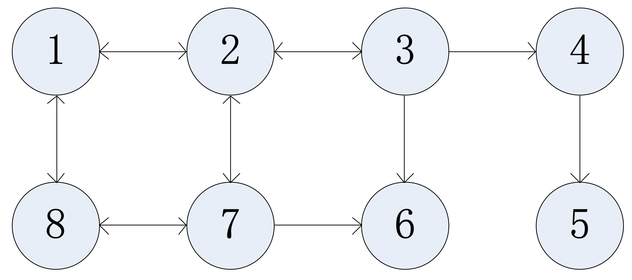
Under the digraph G with 8 agents as shown in Figure 1, numerical simulations of system (1) are executed. In Figure 1, for any $i,j\in \{1,\cdots ,8\}$, if $(i,j)\in E$, then there is a black arrow from the agent i pointing to the agent j.

Figure 1 shows that the digraph G not only contains a spanning tree but also contains a cycle and the adjacency matrix of the digraph G is partible. Hence, the digraph G do not meet the topological assumptions in [25,26]. The communication cycles of agents are all $T=1$ s. When the state of the agent i is updated for the kth time, the distance from the center of mass of the agent i to the starting point is $D_i\left(k\right)$, and $C_{ji}\left(k\right)$ represents the communication distance from the agent i to the agent j, the maximum communication distance between agents is $C_{max}\left(k\right)={max}_{i,j\in V,s\le k}\left\{C_{ji}\left(s\right)\right\}$. The speed of information dissemination is $v(m/s)$. In this paper, it is assumed that the relationship between the time delay and the communication distance is linear, so let $M\left(k\right)=C_{max}\left(k\right)/v$. For multi-agent systems with increasing communication distances (1), by numerically simulating the convergence of the system (1) under four different conditions where the growth rate of the communication distances is different, the conclusions of this paper are verified.

Among the four simulations, the first three simulations all use eight agents to explore a wide area from the same point, and each agent is responsible for a fan-shaped area with an angle of $\pi /4$. Record the starting point as the origin. In the simulation (1), for any integer $k\ge 0$ and any $i\in V$, $D_i^{\left(1\right)}\left(k\right)=\frac{v}{2}(-{log}_a{k}^b)$, where $a\in (0,\tilde{c})$, $b\in \left(0,\frac{1}{2n}\right)$. Therefore, there exist $a_1\in (0,\tilde{c})$ and $b_1\in \left(0,\frac{1}{2n}\right)$ such that the maximum communication distance of the system satisfies $C_{max}^{\left(1\right)}\left(k\right)=v\ast (-{log}_{a_1}{k}^{b_1})$. This system can be described as a system (1) with an unbounded maximum delay $M_1\left(k\right)$. In the simulation (2), for any integer $k\ge 0$ and any $i\in V$, $D_i^{\left(2\right)}\left(k\right)=\frac{v{d}_{2}k}{2}$, where $d_2\in (0,1)$. Therefore, there exists $d_2^{\prime }\in (0,1)$ such that the maximum communication distance of the system satisfies $C_{max}^{\left(2\right)}\left(k\right)=v{d}_2^{\prime }k$. The system can be described as a system (1) with an unbounded maximum delay $M_2\left(k\right)$. In the simulation (3), for any integer $k\ge 0$ and any $i\in V$, $D_i^{\left(3\right)}\left(k\right)=\frac{v}{2}(-{log}_a\left(k^{b/2}\right))$. Therefore, there exist $a_3=a_1$ and $b_3=b_1/2$ such that the maximum communication distance of the system satisfies $C_{max}^{\left(3\right)}\left(k\right)=v\ast (-{log}_{a_3}{k}^{b_3})$. The system can be described as a system (1) with an unbounded maximum delay $M_3\left(k\right)$. The simulation (4) uses 8 agents to explore in a circle with a diameter of $v\left(m\right)$. The starting points of agents are 8 octsection points on the circle, and each agent is responsible for the fan-shaped area with an angle of $\pi /4$. The agent finally converges at the center of the circle. Then, for any integer $k\ge 0$ and any $i\in V$, $D_i^{\left(4\right)}\left(k\right)=v-d_{4}vk$, where $d_4>0$, and satisfies $D_i^{\left(4\right)}\left(k\right)\ge 0$. Therefore, the maximum communication distance of the system satisfies $C_{max}^{\left(4\right)}\left(k\right)\le 2v$. This system can be described as a system (1) with a bounded maximum delay $M_4\left(k\right)$. It can be noticed that in the first three simulations, the maximum communication distance $C_{max}^{\left(1\right)}\left(k\right)$, $C_{max}^{\left(2\right)}\left(k\right)$ and $C_{max}^{\left(3\right)}\left(k\right)$ tends to infinity as the number of iterations k growths, and the maximum communication distance $C_{max}^{\left(4\right)}\left(k\right)$ in the simulation (4) is bounded.

Figure 2 describes the motion trajectories of eight agents in four simulations, in which the abscissa and ordinate describe the position of any point in the two-dimensional plane, and the unit is m. The colored curves are the motion trajectories of all agents. Starting from the purple trajectory and rotating clockwise to the green trajectory, corresponding agent numbers are $1,2,3,4,5,6,7,8$, respectively; and the black dashed line is used to separate the detection areas of the eight agents. In Figure 2, the circle enclosed by the black dashed line in the sub-figure simulation (4) is the boundary of the detection area in the simulation (4).

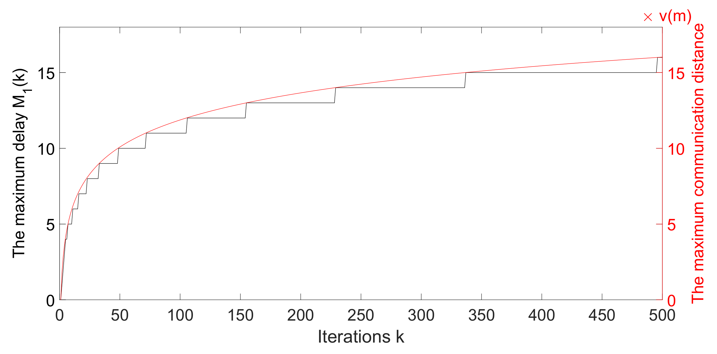
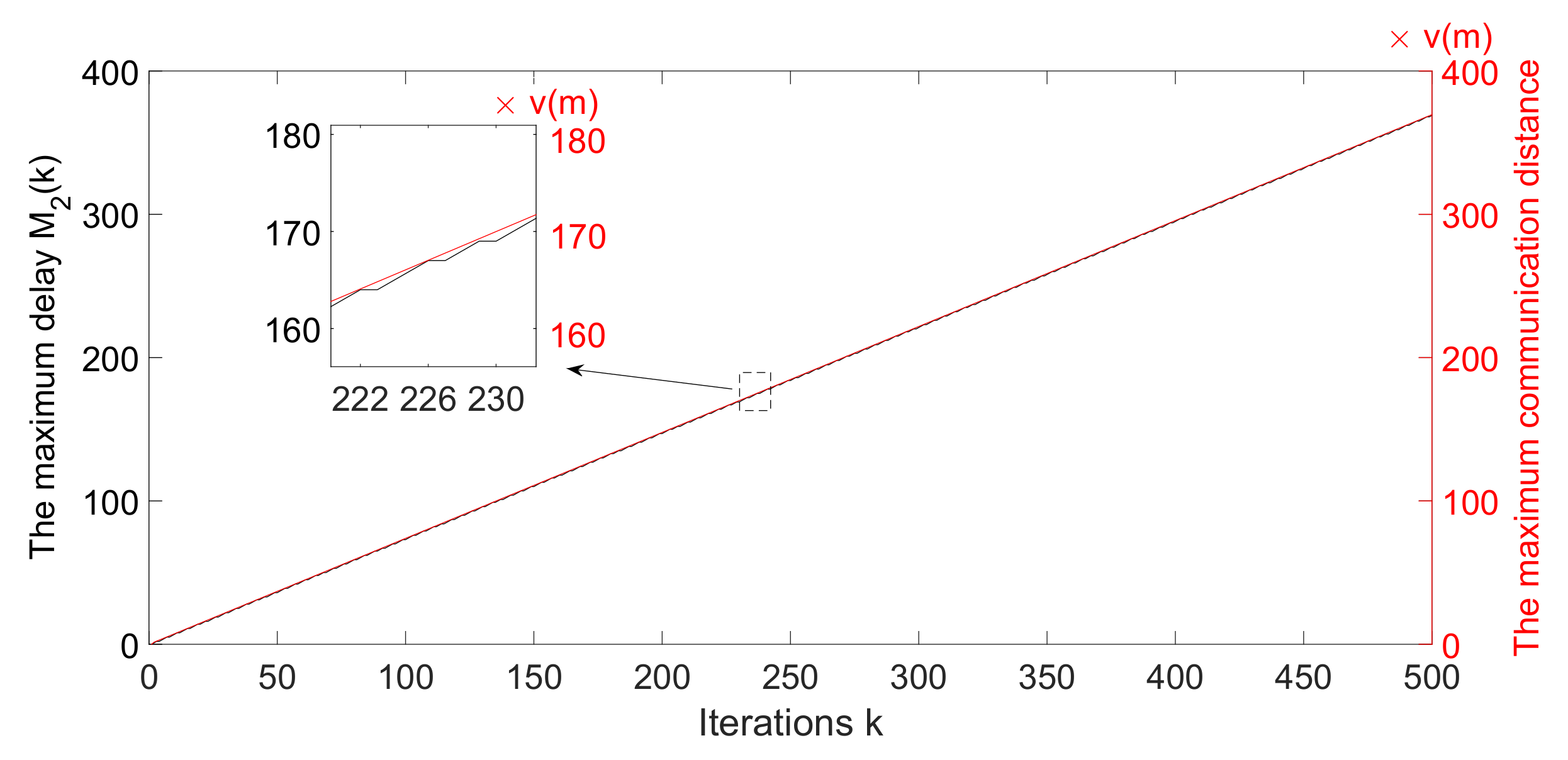
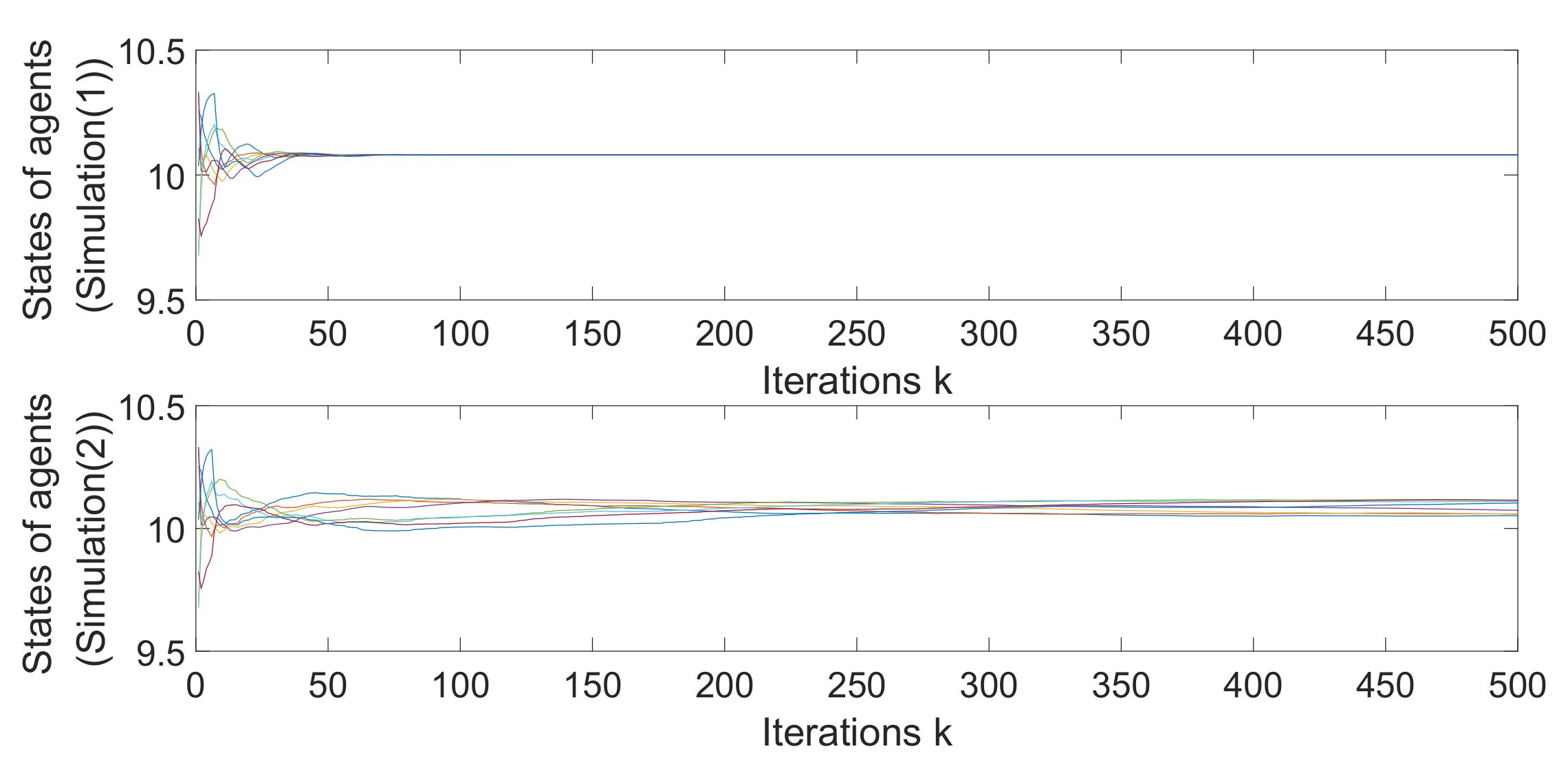
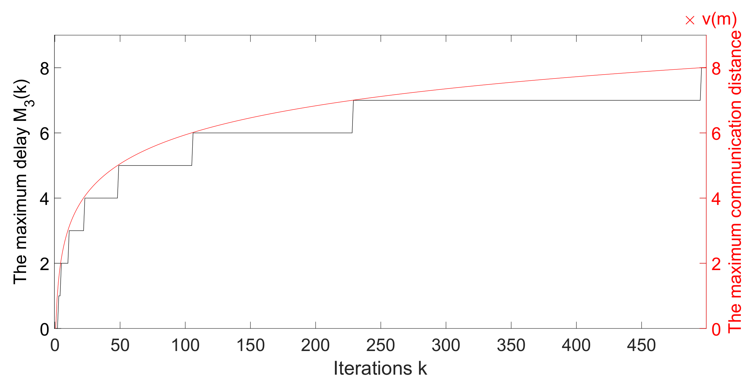
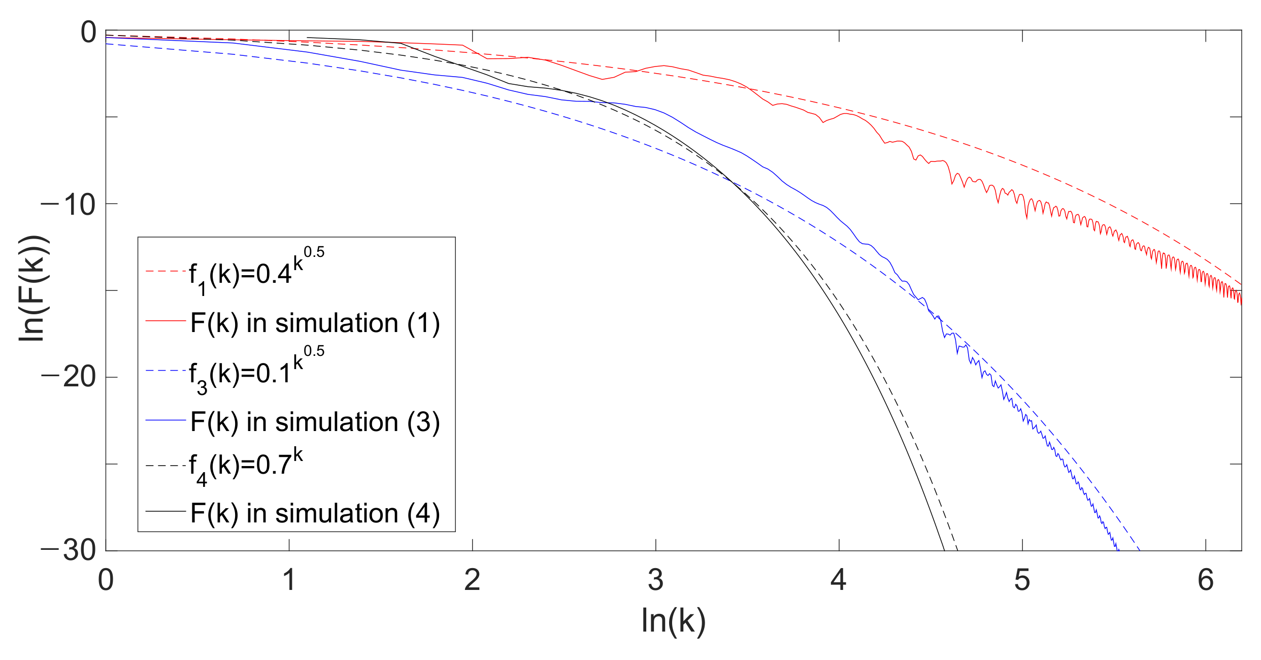
Figure 3, Figure 4, Figure 6 and Figure 7 show the variation of the maximum communication distances between agents $C_{max}^{\left(s\right)}\left(k\right),s=1,2,3,4$ and the maximum delays $M_s\left(k\right),s=1,2,3,4$ with the number of iterations k of four simulations, respectively. It can be seen that the maximum communication distance $C_{max}\left(k\right)$ and the maximum communication delay $M\left(k\right)$ meet the same changing trend. Figure 5 is a comparison figure of change curves of the agent state value in the simulation (1) and the simulation (2). Figure 8 describes the logarithmic function curve of the state error between the agents in the simulation (1), the simulation (3) and the simulation (4) in logarithmic coordinates.

First, compare the simulation (1) and the simulation (2). Since the growth rate of $D_i^{\left(2\right)}\left(k\right)$ in the simulation (2) is faster than the growth rate of $D_i{\left(k\right)}^{\left(1\right)}$ in the simulation (1), Figure 2 shows that the range of agent detection in the simulation (2) obviously exceeds the range of agent detection in the simulation (1).

Figure 3 shows that since the maximum communication distance satisfies $C_{max}^{\left(1\right)}\left(k\right)=v\ast (-{log}_{a_1}{k}^{b_1})$, the curve of the maximum communication delay $M_1\left(k\right)$ closely follows the logarithmic function curve $g_1\left(k\right)=-{log}_{a_1}{k}^{b_1}$. Figure 4 shows that since the maximum communication distance satisfies $C_{max}^{\left(2\right)}\left(k\right)=v{d}_2^{\prime }k$, the curve of the maximum communication delay $M_2\left(k\right)$ closely follows the linear function curve $g_2\left(k\right)=d_2^{\prime }k$. Therefore, the unbounded maximum delay $M_1\left(k\right)$ satisfies the condition in Corollary 2, and the unbounded maximum delay $M_2\left(k\right)$ only satisfies Assumption 2.

Figure 5 shows that the system with the maximum delay $M_1\left(k\right)$ is convergent, but the system with the maximum delay $M_2\left(k\right)$ is divergent. In other words, when the growth rate of the maximum communication distance can ensure that the maximum delay satisfies both Assumption 2 and Assumption 3, the system (1) can reach a consensus under Assumption 1 for topology, which is more relaxed than the topological assumptions in [25,26].

Next, compare the simulation (1), the simulation (3) and the simulation (4). Since $D_i^{\left(1\right)}\left(k\right)$ growths faster than $D_i^{\left(3\right)}\left(k\right)$, Figure 2 shows that the detection range of agents in the simulation (1) is larger than the detection range of agents in the simulation (3). Furthermore, since $D_i^{\left(3\right)}\left(k\right)$ increases with the growth of k, $D_i^{\left(4\right)}\left(k\right)$ decreases with the growth of k, there exists $K>0$ such that $D_i^{\left(3\right)}\left(k\right)>D_i^{\left(4\right)}\left(k\right)$ for all integers $k>K$. In other words, due to the limited detection range of the simulation (4), as long as the detection time is long enough, the detection range of agents in the simulation (1) and the simulation (3) will always be larger than the detection range of agents in the simulation (4).

Figure 6 shows that due to the maximum communication distance satisfies $C_{max}^{\left(3\right)}\left(k\right)=v\ast (-{log}_{a_3}{k}^{b_3})$, the curve of the maximum communication delay $M_3\left(k\right)$ closely follows the logarithmic function curve $g_3\left(k\right)=-{log}_{a_3}{k}^{b_3}$. Therefore, the unbounded maximum delay $M_3\left(k\right)$ satisfies the condition in Corollary 2. Figure 7 shows that due to the maximum communication distance satisfies $C_{max}^{\left(4\right)}\left(k\right)\equiv v$, the curve of the maximum communication delay $M_3\left(k\right)$ satisfies $M_4\left(k\right)\equiv 1$, which is bounded. In other words, the unbounded maximum delay $M_4\left(k\right)$ satisfies the condition in Corollary 1. Obviously, the maximum delay in the simulation (1), the simulation (3) and the simulation (4) satisfies that the growth rate of $M_1\left(k\right)$ is greater than the growth rate of $M_3\left(k\right)$, and the growth rate of $M_3\left(k\right)$ is greater than the growth rate of $M_4\left(k\right)$.

Figure 8 describes the system error curve $F\left(k\right)=\parallel {max}_{i,j}\{x_i\left(k\right)-x_j\left(k\right)\}\parallel$ in the simulation (1), the simulation (3) and the simulation (4) under logarithmic coordinates $ln\left(k\right)-ln\left(F\right(k\left)\right)$. In Figure 8, the curve of the function $f_1\left(k\right)=0.4^{\sqrt{k}}$ in logarithmic coordinates is a red dashed line, the curve of the function $f_3\left(k\right)=0.1^{\sqrt{k}}$ in logarithmic coordinates is a blue dashed line, and the curve of the function $f_4\left(k\right)=0.7^k$ in logarithmic coordinates is a black dashed line. The red solid line is the $F\left(k\right)$ of the system (1) with the unbounded maximum delay $M_1\left(k\right)$. It is below the red dashed line $f_1\left(k\right)$, indicating that the convergence rate of the system (1) with the unbounded maximum delay $M_1\left(k\right)$ is $\mathrm{O}\left(0.4^{\sqrt{k}}\right)$, and the system is asymptotically convergent. The blue solid line is the $F\left(k\right)$ of the system (1) with the unbounded maximum delay $M_3\left(k\right)$. It is below the blue dashed line $f_3\left(k\right)$, indicating that the convergence rate of the system (1) with the unbounded maximum delay $M_3\left(k\right)$ is $\mathrm{O}\left(0.1^{\sqrt{k}}\right)$. In other words, the system (1) with unbounded maximum delay $M_3\left(k\right)$ is asymptotically convergent and has a faster convergence rate than the convergence rate of the system (1) with unbounded maximum delay $M_1\left(k\right)$. The black solid line is the $F\left(k\right)$ of the system (1) with the unbounded maximum delay $M_4\left(k\right)$. It is below the black dashed line $f_4\left(k\right)$, indicating that the convergence rate of the system (1) with the unbounded maximum delay $M_4\left(k\right)$ is $\mathrm{O}\left(0.7^k\right)$, which is exponential. It is faster than the convergence rate of the system (1) in simulation (1) and simulation (3). Therefore, the comparison simulation supports the conclusion of Theorem 4 the the convergence rate of the system (1) is negatively correlated with the growth rate of the maximum delay.

5. Conclusions

In this paper, the consensus problem of multi-agent systems is studied with non-distributed unbounded time-delays caused by the growth of communication distances. The multi-agent system is modeled as a discrete time-delay system. Then, for any finite integer $k>0$, the finite-dimensional augmented model of the time-delay system is built in the interval $[0,k]$ to study the system state. Firstly, under the topology containing a spanning tree and a mild condition about the growth rate of the maximum delay, which also is a constraint on the growth rate of the maximum communication distance, the system is proved to achieve a consensus. Then, this paper shows that the rate of the system achieving a consensus and the growth rate of the maximum delay are negatively correlated. Furthermore, the rate of the system achieving a consensus and the growth rate of the maximum communication distance also satisfy the same relationship. It is worth noting that these results are applicable to any multi-agent system that can be described as the discrete system with non-distributed unbounded time-varying delays. Furthermore, in the future research, we will study the influence of the unbounded delay containing the transmutation delay and the a process scheduling delay on the modeling and consensus conditions of the system. It is foreseeable that the research results will be applicable to a wider range of practical systems.

References

- Lin, Z.; Wang, L.; Chen, Z.; Fu, M.; Han, Z. Necessary and sufficient graphical conditions for affine formation control. IEEE Trans. Autom. Control 2016, 61, 8277–8291. [Google Scholar] [CrossRef]
- Dong, C.; Zhang, W.; Wang, Q.; Liu, Y. Time-varying anti-disturbance formation control for high-order non-linear multi-agent systems with switching directed topologies. IET Control Theory Appl. 2020, 14, 271–282. [Google Scholar] [CrossRef]
- Schenato, L.; Fiorentin, F. Average TimeSynch: A consensus-based protocol for clock synchronization in wireless sensor networks. Automatica 2011, 47, 1878–1886. [Google Scholar] [CrossRef]
- He, J.; Cheng, P.; Shi, L.; Chen, J.; Sun, Y. Time synchronization in WSNs: A maximum-value-based consensus approach. IEEE Trans. Autom. Control 2014, 59, 660–675. [Google Scholar] [CrossRef]
- Tian, Y.P. Time synchronization in WSNs with random bounded communication delays. IEEE Trans. Autom. Control 2017, 62, 5445–5450. [Google Scholar] [CrossRef]
- Olfati-Saber, R.; Murray, R.M. Consensus problems in networks of agents with switching topology and time-delays. IEEE Trans. Autom. Control 2004, 49, 1520–1533. [Google Scholar] [CrossRef] [Green Version]
- Ren, W.; Beard, R.W.; McLain, T.W. Coordination variables and consensus building in multiple vehicle systems. Lecture Notes Control Inf. Sci. 2005, 309, 171–188. [Google Scholar]
- Song, X.; Zhao, P.; Xing, Z.; Peng, J. Global asymptotic stability of cnns with impulses and multi-proportional delays. Math. Methods Appl. Sci. 2016, 39, 722–733. [Google Scholar]
- Wan, P.; Jian, J. Global convergence analysis of impulsive inertial neural networks with time-varying delays. Neurocomputing 2017, 245, 68–76. [Google Scholar] [CrossRef]
- Tu, Z.; Cao, J.; Alsaedi, A.; Alsaadi, F. Global dissipativity of memristor-based neutral type inertial neural networks. Neural Netw. 2017, 88, 125–133. [Google Scholar] [CrossRef]
- Tian, Y.P.; Chun, S.; Chen, G.; Zong, S.; Huang, Y.; Wang, B. Delay compensation based time synchronization under random delays: Algorithm and experiment. IEEE Trans. Control Syst. Technol. 2021, 29, 80–95. [Google Scholar] [CrossRef]
- Tilak, S.; Abu-Ghazaleh, N.; Heinzelman, W. Infrastructure tradeoffs for sensor networks. In Proceedings of the 1st ACM International Workshop on Wireless Sensor Networks and Applications, Atlanta, GA, USA, 28 September 2002; pp. 49–58. [Google Scholar]
- Zhang, W.A.; Yu, L. Stability analysis for discrete-time switched time-delay systems. Automatica 2009, 45, 2265–2271. [Google Scholar] [CrossRef]
- Hou, W.; Fu, M.; Zhang, H. Consensusability of linear multi-agent systems with time delay. Int. J. Robust Nonlinear Control 2017, 26, 2529–2541. [Google Scholar] [CrossRef]
- Xiao, F.; Wang, L. Consensus protocols for discrete-time multi-agent systems with time-varying delays. Automatica 2008, 44, 2577–2582. [Google Scholar] [CrossRef]
- Kaviarasan, B.; Sakthivel, R.; Li, Y.; Zhao, D.; Ren, Y. Non-fragile control protocol for finite-time consensus of stochastic multi-agent systems with input time-varying delay. Int. J. Mach. Learn. Cybern. 2020, 11, 325–337. [Google Scholar] [CrossRef]
- Liang, S.; Liu, Z.; Chen, Z. Leader-following exponential consensus of discrete-time multi-agent systems with time-varying delay and intermittent communication. Int. J. Control Autom. Syst. 2019, 17, 1–11. [Google Scholar] [CrossRef]
- Chen, Y.; Lam, J.; Cui, Y.; Kwok, K.W. Switched systems approach to state bounding for time delay systems. Inf. Sci. 2018, 465, 191–201. [Google Scholar] [CrossRef]
- Michiels, W.; Morǎrescu, C.I.; Niculescu, S.I. Consensus problems with distributed delays, with application to traffic flow models. SIAM J. Control Optim. 2009, 48, 77–101. [Google Scholar] [CrossRef]
- Xu, X.; Feng, G. Consensus of linear multi-agent systems with distributed infinite transmission delays: A low gain method. In Proceedings of the 2018 37th Chinese Control Conference (CCC), Wuhan, China, 25–27 July 2018; Volume 48, pp. 6645–6652. [Google Scholar]
- Josić, K.; López, J.M.; Ott, W.; Shiau, L.; Bennett, M.R. Stochastic delay accelerates signaling in gene networks. PLoS Comput Biol. 2011, 7, e1002264. [Google Scholar] [CrossRef] [Green Version]
- Liu, B.; Lu, W.; Chen, T. Generalized Halanay inequalities and their applications to neural networks with unbounded timevarying delays. IEEE Trans. Neural Netw. 2011, 22, 1508–1513. [Google Scholar] [CrossRef]
- Pathirana, P.N.; Nam, P.T.; Trinh, H.M. Stability of positive coupled differential-difference equations with unbounded time-varying delays. Automatica 2018, 92, 259–263. [Google Scholar] [CrossRef]
- Li, H.; Zhang, W.; Li, C.; Zhang, W. Global asymptotical stability for a class of non-autonomous impulsive inertial neural networks with unbounded time-varying delay. Neural Comput. Appl. 2019, 31, 6757–6766. [Google Scholar] [CrossRef]
- Liu, X.; Lu, W.; Chen, T. Consensus of multi-agent systems with unbounded time-varying delays. IEEE Trans. Autom. Control 2010, 55, 2396–2401. [Google Scholar] [CrossRef]
- Xiang, X.; Lu, L.; Gang, F. Consensus of single integrator multi-agent systems with unbounded transmission delays. J. Syst. Sci. Complex. 2019, 32, 778–788. [Google Scholar]
- Zong, S.; Tian, Y.P. Consensus of discrete-time multi-agent systems with unbounded time-varying delays. In Proceedings of the 39th Chinese Control Conference (CCC), Shenyang, China, 27–29 July 2020. [Google Scholar]
Figure 1.
The topology graph G with 8 agents.
Figure 2.
The motion trajectories of 8 agents.
Figure 3.
The maximum communication distances between agents and the maximum delays in the simulation (1).
Figure 4.
The maximum communication distances between agents and the maximum delays in the simulation (2).
Figure 5.
The state change curve of agents in the simulation (1) and the simulation (2).
Figure 6.
The maximum communication distances between agents and the maximum delays in the simulation (3).
Figure 7.
The maximum communication distances between agents and the maximum delays in the simulation (4).
Figure 8.
The system error curve in the simulation (1), the simulation (3) and the simulation (4) under logarithmic coordinates.
Publisher’s Note: MDPI stays neutral with regard to jurisdictional claims in published maps and institutional affiliations. |
© 2021 by the authors. Licensee MDPI, Basel, Switzerland. This article is an open access article distributed under the terms and conditions of the Creative Commons Attribution (CC BY) license (https://creativecommons.org/licenses/by/4.0/).
Share and Cite
MDPI and ACS Style
Zong, S.; Tian, Y.-P. Consensus of Multi-Agent Systems with Unbounded Time-Varying Delays. Appl. Sci. 2021, 11, 4944. https://doi.org/10.3390/app11114944
AMA Style
Zong S, Tian Y-P. Consensus of Multi-Agent Systems with Unbounded Time-Varying Delays. Applied Sciences. 2021; 11(11):4944. https://doi.org/10.3390/app11114944
Chicago/Turabian StyleZong, Siheng, and Yu-Ping Tian. 2021. "Consensus of Multi-Agent Systems with Unbounded Time-Varying Delays" Applied Sciences 11, no. 11: 4944. https://doi.org/10.3390/app11114944
Note that from the first issue of 2016, this journal uses article numbers instead of page numbers. See further details here.