Multiscale Post-Seismic Deformation Based on cGNSS Time Series Following the 2015 Lefkas (W. Greece) Mw6.5 Earthquake

Abstract

In the present work, a multiscale post-seismic relaxation mechanism, based on the existence of a distribution in relaxation time, is presented. Assuming an Arrhenius dependence of the relaxation time with uniform distributed activation energy in a mesoscopic scale, a generic logarithmic-type relaxation in a macroscopic scale results. The model was applied in the case of the strong 2015 Lefkas Mw6.5 (W. Greece) earthquake, where continuous GNSS (cGNSS) time series were recorded in a station located in the near vicinity of the epicentral area. The application of the present approach to the Lefkas event fits the observed displacements implied by a distribution of relaxation times in the range τ_min ≈ 3.5 days to τ_max ≈ 350 days.

1. Introduction

Earthquake rupture creates static stress changes within the lithosphere that are large enough to produce transient deformation that can be observed on the Earth’s surface. Satellite geodesy using GNSS techniques for observing Earth’s surface displacements have advanced in such a level that the post-seismic deformation can be monitored with high accuracy [1].

To study post-seismic relaxation, various mechanisms have been proposed, such as those of poroelasticity of the rock medium [2,3], shallow after-slip on the main faulting plane or nearby faults [4,5], and viscoelastic relaxation [6]. The after-slip mechanisms are localized and follow logarithmic decay [4,7], while the viscoelastic one is supported by a bulk deformation process and exhibits exponential decay [8,9,10].

In [11], it was demonstrated that, during the first 6 months following the 1999 Chi-Chi earthquake (M = 7.6, Taiwan), both the post-seismic relaxation and the cumulative number of aftershocks followed the same temporal dependence, which reduced to a logarithmic one after a long time from the main event. In addition, logarithmic deformation could be explained by an exhaustion process, which is based on the assumption that the number of sources of strain-producing events evolve according to a thermally activated process, in which the activation energy is stress dependent [12].

The recent strong earthquakes present examples where the macroscopic post-seismic deformation is interpreted in view of the above relaxation mechanisms, which are based on the assumption of a single relaxation time estimated for each post seismic relaxation observed [13,14,15,16,17,18].

Experimental results and theoretical models suggest that post seismic relaxation is thermally activated and enhanced by the presence of fluids [19]. Deformation is controlled by a variety of temperature-dependent healing processes that are related to the crack size [20,21]. Since different crack sizes have different activation energy, the associated relaxation processes operate at different timescales [22], indicating an intrinsic organization [23] with a distribution of relaxation times, instead of the use of a single one. The latter implies that post-seismic relaxation could be viewed as the superposition of several different relaxation times, each one activated in different mesoscopic domains of the macroscopic relaxed seismic volume. Thus, the macroscopic relaxation observed results from the superposition of different relaxation times on the microscopic–mesoscopic scale, which obviously operates on different spatiotemporal scales. The recovery process that returns the deformed volume to equilibrium after a strong earthquake could be characterized as a slow dynamics process [24], because an instantaneous perturbation causes a transient response, which moves the system to a state of equilibrium [25,26,27,28,29,30]. It is, thus, possible that relaxation, which varies with the logarithm of time, can be interpreted as the result of the superposition of relaxation mechanisms with a spectrum of relaxation times.

The purpose of this work is to give a description of the post seismic deformation relaxation. It is based on the thermodynamic Arrhenius model for the distribution of the relaxation times [31] and describes the post-seismic recovery as a slow thermodynamic process taking place in a mesoscopic scale. The model predicts a physically accepted finite value just after the co-seismic perturbation, a logarithmic time dependence for the time period between the minimum and maximum relaxation time, and an exponential decay while approaching an equilibrium state a long time after the main event. Based on that, the explanation that relaxation occurs as a logarithm of time does not depend on the details of Earth’s physical and chemical properties, but is based on a generic, or even a universal, multiscale property of the relaxation mechanism, as resulted from the Arrhenius expression, which connects relaxation time with the activation energy of the relaxation process.

To test the proposed approach for the post-seismic relaxation, positioning data from the continuous GNSS station PONT [32] and www.geodesy.gein.noa.gr (accessed on 30 December 2020) located in the southern part of Lefkas Island were used. This cGNSS station is located in the close vicinity of the earthquake epicenter of the 17 November 2015 Mw6.5, shallow event (~10 km depth), that occurred on the island, causing severe damages and human losses.

2. A Thermodynamic Model of Post Seismic Relaxation

A post-seismic transient deformation stage, where strain varies with time at a decreasing rate, occurs following the instantaneous deformation during an earthquake. Transient deformation is followed by the return to steady-state deformation, where the strain rate is a constant after some time following the main event.

Following [33], we define a relaxation function R(t), where t is the time after the main seismic event, as a perturbation of the displacement given by the generic expression:

$$u\left(t\right)=u_{\infty }+S R\left(t\right)$$

(1)

where $u_{\infty }$ is the equilibrium value of displacement after a long time and S is a scaling factor. Notice that $R\left(t\to \infty \right)\approx 0,$ while $u_{\infty }=u\left(t\to \infty \right)$ is the remaining distortion at the end of the relaxation process. The initial value $u_o$ of the post-seismic deformation immediately after the co-seismic perturbation δu_c is given from Equation (1) as $u_o=u\left(t=0^{+}\right)=u_{\infty }+S R_O$, where $R_0=R\left(t=0\right)$. The scaling factor S of the relaxation constrains the rheological properties of the medium [34,35] and depends on the rheology of the crust and upper mantle, as well as on the local conditions around the site (i.e., crustal heterogeneities). In addition, S depends on the stress released in the medium and reflects the response of the medium (i.e., of the magnitude of the earthquake event) after the co-seismic displacement due to earthquake.

In most of the cases a simple relaxation mechanism with a single relaxation time τ that corresponds to a relaxation function exp (−t/τ) (i.e., not varying logarithmically with time) is the simplest rheological model introduced to explain post-seismic deformation, known as the linear Maxwell model [6]. In this case:

$$R_o=1,\hspace{1em}\hspace{1em}\hspace{1em}\hspace{1em}{u}_o=u_{\infty }+S{ }_{}\mathrm{and} u\left(t\right)=u_{\infty }+S e^{\raisebox{1ex}{$-t$}\!\left/ \!\raisebox{-1ex}{$\tau $}\right.}$$

(2)

while the normalized displacement is $\mathrm{D}\left(t\right)=\frac{u\left(t\right)}{u_o}=\frac{1+\frac{S}{u_{\infty }}{e}^{\raisebox{1ex}{$-t$}\!\left/ \!\raisebox{-1ex}{$\tau $}\right.} }{1+\frac{S}{u_{\infty }}}$. In Figure 1, we plot the displacement as a function of normalized time $\raisebox{1ex}{$t$}\!\left/ \!\raisebox{-1ex}{$\tau $}\right.$. In the very early stage, expanding the exponential in Equation (2) leads us to $u\left(t\right)=u_{\infty }+S\left(1-\frac{t}{\tau }\right)\mathrm{or}\mathrm{D}\left(t\right)=1-\frac{\frac{S}{u_{\infty }} }{1+\frac{S}{u_{\infty }}} \frac{t}{\tau }$, a linear expression of normalized displacement with time, which for $\frac{S}{u_{\infty }}\gg 1,$ leads to D = 1 − (t/τ) with the slope equal to 1/τ, and independent of S.

We proceeded to study a post-seismic relaxation process with a spectrum of relaxation times within the range defined by the minimum and maximum values ${\tau }_{min}$, ${\tau }_{max}$ of relaxation time, respectively. If f(τ) is the distribution function of the relaxation time, then:

$$R\left(t\right)={{\displaystyle \int }}_{{\tau }_{min}}^{{\tau }_{max}}f\left(\tau \right)e^{\raisebox{1ex}{$-t$}\!\left/ \!\raisebox{-1ex}{$\tau $}\right.}d\tau$$

(3)

The expression (3) is based on the assumption that the total macroscopic relaxation observed is a result of the superposition of relaxation processes operating with different relaxation times τ. This approach could be viewed as a generalization of the Burgers body rheological model [8,36,37], expanding the two discrete relaxation times to a continuum spectrum in the range values ${\tau }_{min}$, ${\tau }_{max}.$

Assuming a relaxation process with activation energy E, then following Arrhenius’ law [31], the relaxation time is given by:

$$\tau ={\tau }_0{e}^{\raisebox{1ex}{$E$}\!\left/ \!\raisebox{-1ex}{$k_{B}T$}\right.}$$

(4)

with ${\tau }_0$ a constant proexponential factor, T the temperature, and k_B the Boltzmann constant. If the activation energy is distributed following a distribution function N(E), then the distribution function f(τ) for the relaxation times satisfies the expression f(τ) =N(E)(dE/dτ). Using Expression (4), dτ/dE= (${\tau }_0$/k_BT)exp (E/k_BT) = τ/k_BT, hence:

$$f\left(\tau \right)=\frac{k_{B}TN\left(E\right)}{\tau }$$

(5)

In the case of a uniform distribution of the activation energy, bounded by a minimum E_min and maximum E_max activation energy, N(E) has a constant value N_o, which, according to Equation (5) for a temperature T, leads to a distribution of relaxation times $f\left(\tau \right)=(k_{B}T{{\rm N}}_0)/\tau ,$ which is proportional to 1/τ. It is evident that the minimum ${\tau }_{min}$ and maximum ${\tau }_{max}$ relaxation times are related to the corresponding minimum and maximum activation energies by the expressions ${\tau }_{min}={\tau }_0{e}^{\raisebox{1ex}{$E_{min}$}\!\left/ \!\raisebox{-1ex}{$k_{B}T$}\right.}$ and ${\tau }_{max}={\tau }_0{e}^{\raisebox{1ex}{$E_{max}$}\!\left/ \!\raisebox{-1ex}{$k_{B}T$}\right.}$ and, thus, $\Delta {\rm E}=E_{max}-E_{min}=kT \ln (\frac{{\tau }_{max}}{{\tau }_{min}}$).

The macroscopically observed relaxation is given by the superposition of relaxation processes, expressed as:

$$R\left(t\right)=C{{\displaystyle \int }}_{{\tau }_{min}}^{{\tau }_{max}}\frac{1}{\tau }{e}^{-t/\tau }d\tau$$

(6)

where C = $T N_o$ is a constant for a given T and N_o, which is omitted in the calculation merging it with the scaling parameter S. We note that N_o is a constant value for a uniform distribution of energy N(E) between its minimum E_min and maximum E_max value. The weight factor 1/τ in Equation (6) is a result of the application of Arrhenius’ law due to mesoscale relaxation processes operating on different timescales. In Figure 2, we present examples of the relaxation function with time on a logarithmic scale along the horizontal axis with a constant ${\tau }_{min}$ and various values of ${\tau }_{max}$. In a logarithmic scale, the curve in Figure 2 decreases almost linearly, up to a time t ≈ τ_max, and at the end, it flattens out. Thus, the relaxation function R(t) is proportional to ln (t) for t << τ_max. Based on that, the maximum relaxation time τ_max could be estimated as the time where the relaxation curve flattens out.

The integral in Equation (6) is the exponential integral E₁(x) [38], which can not be solved analytically but behaves like a negative exponential for very large values of the argument and decays on a logarithmic mode in the intermediate range of the relaxation curve R(t) while deviating from a logarithmic time dependence for t < τ_min. Furthermore, as results from Equation (6) when t = 0, R(t) can be calculated analytically:

$$R_0=R\left(t=0\right)=\ln \left(\frac{{\tau }_{max}}{{\tau }_{min}}\right)$$

(7)

supporting the physical condition to have a finite relaxation function for t = 0. Since $\Delta {\rm E}=E_{max}-E_{min}=kT\ln \left(\frac{{\tau }_{max}}{{\tau }_{min}}\right)=kT{R}_0$, the finite value of the relaxation function for t = 0 is required in order for the energy range $\Delta {\rm E}$ to be a finite quantity. Taking the derivative of R(t) with respect to t, we form the following equation:

$$\frac{dR}{dt}=\frac{1}{t}\left(e^{\raisebox{1ex}{$-t$}\!\left/ \!\raisebox{-1ex}{${\tau }_{min}$}\right.}-e^{\raisebox{1ex}{$-t$}\!\left/ \!\raisebox{-1ex}{${\tau }_{max}$}\right.}\right)$$

(8)

which, for τ_min$\approx$ t≪τ_max, expands exponentially and leads to ${\left[\frac{dR\left(t\right)}{dt}\right]}_{t=0}=-\left(\frac{1}{{\tau }_{min}}-\frac{1}{{\tau }_{max}} \right)$ and

$$R\left(t\right)\approx \ln \left(\frac{{\tau }_{max}}{{\tau }_{min}}\right)-\left(\frac{1}{{\tau }_{min}}-\frac{1}{{\tau }_{max}} \right)t=R_0-\left(\frac{1}{{\tau }_{min}}-\frac{1}{{\tau }_{max}} \right)t$$

(9)

In the observed cases where τ_max ≫ τ_min, the slope of R(t) vs. t at t = 0 is well approximated as ${\left[\frac{dR\left(t\right)}{dt}\right]}_{t=0}=-\frac{1}{{\tau }_{min}}$, while the ratio of the slope to R(0) follows the expression: $\frac{1}{R\left(t=0\right)}{\left[\frac{dR\left(t\right)}{dt}\right]}_{t=0}=\frac{1}{{\tau }_{min}} \ln \left(\frac{{\tau }_{max}}{{\tau }_{min}}\right)=\frac{R_o}{{\tau }_{min}}$.

Introducing expression (9) in (1), the very early stage displacement immediately following the co-seismic one is given by the expression:

$$u\left(t\right)=u_{\infty }+S{R}_0-S\left(\frac{1}{{\tau }_{min}}-\frac{1}{{\tau }_{max}} \right)t=u_o-F_{1}t$$

(10)

where the slope of Equation (10) is $F_1=S\left(\frac{1}{{\tau }_{min}}-\frac{1}{{\tau }_{max}} \right)\approx S/{\tau }_{min}$ for ${\tau }_{min}\ll {\tau }_{max}$ and $u_o=u_{\infty }+S{R}_0$.

In the case when τ_min ≪ τ_max and the time t is such that τ_min ≪ t ≪ τ_max, we could approximate exponentials such as $e^{\raisebox{1ex}{$-t$}\!\left/ \!\raisebox{-1ex}{${\tau }_{min}$}\right.}\approx 0 \mathrm{and} e^{\raisebox{1ex}{$-t$}\!\left/ \!\raisebox{-1ex}{${\tau }_{max}$}\right.}\approx 1$ and Equation (8) results to:

dR/dt ≈ −1/t

which, after integration, gives:

R(t) ≈ R₁ − ln(t) for τ_min≪τ≪τ_max

(11)

with R₁ an integration constant. Equation (12) reveals that the relaxation function R(t) exhibits a logarithmic behavior in an intermediate time interval bounded by the relaxation times ${\tau }_{min}$ and ${\tau }_{max}$ with a slope −1 in a graph of R(t) versus ln (t). It becomes evident that when multiplying R(t) with a scale factor S in Equation (1), there is a modification of the slope of the postseismic relaxation versus ln (t) related to the particular characteristics of earthquake event and the seismotectonic settings and the rheology of the deformed zone as well. Substituting Equation (11) into (1), displacement obtains logarithmic behavior:

$$u\left(t\right)=u_{\infty }+S{R}_1-S\ln t$$

(12)

for τ_min ≪ τ ≪ τ_max with a slope F₂ = S.

Defining τ* as the point where the transition from the linear to logarithmic behavior starts, there is a continuation of displacement (as given by Equations (10) and (12), respectively), that permits the estimation of R₁ as:

$$R_1=\ln \left(\frac{{\tau }_{max}}{{\tau }_{min}}\right)+\ln {\tau }^{ *}-\left(\frac{1}{{\tau }_{min}}-\frac{1}{{\tau }_{max}} \right){\tau }^{ *}$$

(13)

In order to estimate the order of magnitude of R₁, we calculate its value for two reasonable values of τ*, as that of ${\tau }^{*}={\tau }_{min}$ and ${\tau }^{*}=2{\tau }_{min}$. For ${\tau }^{*}={\tau }_{min},$(i.e., the transition in the logarithmic range starts in the very early stage of deformation), we have $R_1=\ln {\tau }_{max}-1+\frac{{\tau }_{min}}{{\tau }_{max}},$ which for $\frac{{\tau }_{min}}{{\tau }_{max}} \ll 1,$ leads to:

$$R_1=\ln {\tau }_{max}-1$$

giving $R=-\ln \left(\frac{t}{{\tau }_{max}}\right)-1$. Since R(t) is positively defined, the above expression is valid for t < τ_max/e ≈ 0.37${\tau }_{max}$. For a more reasonable estimation, we set ${\tau }^{*}=2{\tau }_{min}$, leading to $R_1=\ln {\tau }_{max}+\ln 2-2(1-\frac{{\tau }_{min}}{{\tau }_{max}}),$ which for $\frac{{\tau }_{min}}{{\tau }_{max}}\ll 1,$ leads to:

$$R_1=\ln {\tau }_{max}+\ln 2-2,$$

with $R=-\ln \left(\frac{t}{{\tau }_{max}}\right)+\ln 2-2.$ From the positive definition of R(t), we conclude that the above expression is valid for $t<\frac{{\tau }_{max}}{2-\ln 2} \approx 0.76{\tau }_{max}$. A comparison between Equations (10) and (13) indicates that the slope of the logarithmic part $F_2=S$ is scaled with that of early stage deformation behavior $F_1=S\left(\frac{1}{{\tau }_{min}}-\frac{1}{{\tau }_{max}} \right).$ For τ_min ≪ τ_max, this scaling can provide an estimation of τ_min, since $\frac{F_2}{F_1}={\tau }_{min}$.

Analyzing the relaxation function (3) for the case τ_min ≪ τ_max ≪ t, the long time behavior of R(t) can be estimated, replacing the upper limit τ_max with infinity so that [33]

$$R\left(t\right)\approx \frac{{\tau }_{max}}{t}{e}^{-\raisebox{1ex}{$t$}\!\left/ \!\raisebox{-1ex}{${\tau }_{max}$}\right.}$$

(14)

indicating that, for t ≫ τ_min, the relaxation function is controlled only by τ_max and not τ_min. In that case, the relaxation time τ_max is predominant, and R(t) leads to $R\left(t\right)=e^{\raisebox{1ex}{$(-t$}\!\left/ \!\raisebox{-1ex}{${\tau }_{max}$}\right.)},$ implying that the term τ_max/t is associated to the relaxation processes with relaxation time τ_min < τ < τ_max. We note that, since the time dependence of 1/t is slow compared to $e^{\raisebox{1ex}{$(-t$}\!\left/ \!\raisebox{-1ex}{${\tau }_{max}$}\right.)},$ the relaxation function could be well approximated as an exponential a long time after the main event. Furthermore, the exponential relaxation, as presented in Equation (2), is a special case of the general expression of the relaxation function (3) and results when τ_min and τ_max have similar values, i.e., when τ_min = τ₀ − Δ and τ_max= τ₀ + Δ, which leads to $R\left(t\right)\approx \frac{2\Delta }{{\tau }_o}{e}^{-\raisebox{1ex}{$t$}\!\left/ \!\raisebox{-1ex}{${\tau }_0$}\right.}$ presenting an exponential decay over time.

3. Seismotectonic Setting, Data Selection, and Analysis

Intense seismic activity in the Central Ionian Islands of Cephalonia and Lefkas during the last few years, along with several large events (M > 6) over the last century [39,40], clearly highlight the key role of this area in the kinematic process in the Eastern Mediterranean. The area is dominated by a major regional seismogenic zone known as the Cephalonia Transform Fault (CTF) (Figure 3), as well as several other faulting features, resulting in generation of the highest seismic energy release in Europe [41,42]. The broader area is characterized by a complex kinematic and geodynamic regime. The area links the oceanic subduction boundary in the south to the collision between the Apulian microplate and Eurasia in the north [43,44,45]. This complicated tectonic regime creates a stress field that generates intense seismic activity and ground deformation on both a local and regional scale.

Based on seismological data and geodetic measurements, the CTF zone is described as a dextral strike-slip faulting type system. This system is composed of two separate segments that run along the western shores of the Cephalonia and Lefkas Islands. The southern segment, offshore of Cephalonia, extends for approximately 90 km on a SW–NE direction and ends on the northern part of the island. The northern segment, offshore of western Lefkas Island, strikes a NE–SW direction for ~50 km, ending close to north-western Cephalonia. This segment dips to the ESE and exhibits dextral strike-slip motion combined with a small thrust component [45].

Over the last twenty years, several strong earthquakes have devastated the islands of Lefkas and Cephalonia. In August 2003, a strong event (M_w6.3) occurred off-shore of the north-western coast of Lefkas Island [46,47,48,49,50]. In late January–early February 2014, two large-magnitude earthquakes (M_w5.9 and M_w6.1) were located in the western part of Cephalonia [51,52]. However, these events were not linked directly with the CTF zone.

This study focuses on a strong seismic event that took place in near proximity to the PONT continuous GNSS station. On 17 November 2015, a strong earthquake (M_w6.4) occurred in the southern part of Lefkas Island [53,54] just north of Cephalonia. The main event was followed by a significant post-seismic activity that extended southwards towards Cephalonia. The hypocenter of this earthquake was located at a depth of ~10 km, and the fault plane solutions demonstrated a NNE–SSW striking dextral strike-slip seismic fault with a reverse component that dipped east at a high angle of about 70° ± 5°. The after-shock seismic activity extended along three distinctive clusters north and south of the main event [54]. The northern cluster seemed to extends towards the epicentral area of the 2003 strong earthquake, the central one was located in the vicinity of the main event, while the southern one extended towards Cephalonia Island and about 15 km southwest of the epicenter. The spatial coverage of the aftershocks indicated less dense distribution close to the epicentral area, while away from the main shock, there was higher concentration of post-seismic activity. The latter may indicate that, during the main event, higher energy was released in the main ruptured fault, which comprised part of the major CTF zone, while the post-seismic activity was triggered in nearby secondary and adjacent local faults, away from the main rupture plain [54]. The post seismic events extended in a NE–SW direction for approximately 50 km, extending north towards the 2003 earthquake and south towards the northern Cephalonia. The southern seismic cluster occurred in the same area that was also activated during all the previous intense seismic periods in 2003 and in 2014 [48,49].

3.1. GNSS Data Analysis

The epicentral area of the 2015 Lefkas earthquake, located to the southern part of the island, is remarkably close to the local continuous GNSS station PONT [32]. This station has been operating in the area since 2007. The GNSS data are processed daily, using 30 s RINEX files, in order to calculate the daily coordinates of the station (Figure 4). From the time series of PONT station coordinates, the station velocity was estimated for the period 2009–2015. Prior to the 2015 strong event, the station exhibited the anticipated regional motion of the area, and the velocity was calculated as V_East = (20.45 ± 0.03) mm/yr, V_North = (6.81 ± 0.02) mm/yr, and V_Up = (−0.71 ± 0.08) mm/yr with respect to IGb08 reference frame (http://igscb.jpl.nasa.gov/network/refframe.html) (accessed on 30 December 2020). The earthquake of 17 November 2015 caused a co-seismic displacement of the PONT station of 360 mm to south, 201 mm to the west, and a subsidence of 73 mm (Figure 4).

The files from PONT station were processed using the Bernese Software version 5.2 [55]. The software allows the estimation of epoch wise receiver coordinates in precise point positioning mode (PPP), as well as in the double difference mode. For the present research, coordinates were calculated after the earthquake of 2015 on a static mode. To get the best results, the PPP technique was used as a first step to get a priori coordinate values, which were, consequently, introduced in the more precise double difference method. In the processing procedure, GNSS data from 25 IGS and EUREF cGNSS stations from Europe, Greece, Cyprus, and Turkey were used to define the local reference frame. Ambiguities were solved using several resolution strategies depending on the baseline length between the stations: the wide-lane and narrow-lane for the medium baseline (<10–200 km) and the quasi-ionosphere-free (QIF) strategy for long baselines (<1000–2000 km). For the troposphere modelling, the dry and wet Vienna mapping function (VMF) of Bohm et al. (2006), the dry and wet Niell model [56], as well as the Saastamoinen model [57] were the models used to analyze the GNSS microwave data in different stages of the processing. Effects of the solid earth tides were taken into account and corrections of the ocean tide loading were applied based on the FESS2004 model. In analogy to site displacements caused by ocean tide loading, the loading effect of the atmospheric tides were taken into account in the processing of the GNSS data. The latter was done by introducing a specific file in the processing containing atmospheric tidal loading coefficients from a global grid-based model [58]. Moreover, the absolute antenna phase center corrections were used in the processing and to better improve the final solutions files containing the precise orbital parameters; the Earth orientation parameters and the satellite clock corrections were taken from the Center for Orbit Determination in Europe (CODE) (DOI:10.7892/boris.75876.4). On a weekly basis, the calculated coordinates were evaluated for the repeatability error, and in case of large deviations from the weekly solution, the values were excluded. The latter resulted in an unweighted RMS error, in mm, for each component that varied from 0.5 to 1.01 in the east component, 0.8 to 2.1 in the north one, and 1.8 to 4.6 for the up component. However, that was not applied for the first ten days after the main event. The daily coordinates were estimated with respect to IGb08 reference frame.

3.2. Post Seismic Time Series Analysis

The post seismic displacement evolution is made up of two contributions: the displacement u(t) due to the relaxation one on the fault zone and the long term V_pst t, where V_pst is the long term loading velocity a long time after the earthquake when the system has reached a new equilibrium state. In our case, V_pstEast = (17.48 ± 0.07) mm/yr, V_pstNorth = (3.72 ± 0.07) mm/yr, and V_pstUp = (−0.44 ± 0.18) mm/yr, which was removed from the observed postseismic data. To apply our approach, we analyzed the post seismic relaxation observed after the 17 November 2015 Mw6.5, Lefkas island earthquake. In Figure 5, the North–South displacement, which was the event’s predominant post seismic displacement, presented as a function of time for a period 1000 days after the event. For energy reasons, the minimum relaxation time τ_min cannot be equal to zero in order to have a converged relaxation function. From Figure 5, the transition from the linear to logarithmic part is observed, permitting the estimation of τ_min ≈ 3–5 days. Since the longest relaxation time τ_max is the time where the relaxation stops, from Figure 5, we estimate τ_max ≈ 350 days. The aforementioned estimations of τ_min and τ_max result in a value R_o ≈ 4.2 to 4.7. Using the observed values of $u\left(t\right),$ we estimate that an average value of displacement in the range from 300 to 600 days is about −26 mm, a value that could be used to approximate $u_{\infty }.$ In Figure 5, the observed displacement, along with the theoretical one, calculated using Equation (1), with S = 4.8 mm, $u_{\infty }=-26 \mathrm{mm}$, τ_min ≈ 3.5 days, and τ_max ≈ 350 days (i.e., R_o ≈ 4.6), is presented as a very good agreement. Furthermore, the time evolution of displacement suggests a slope F₂ ≈ −4.21 for the logarithmic part and an approximate value F₁ ≈ −1.09 for the short linear early part of deformation. Comparing the above estimation with Equations (10) and (13), we conclude that, since τ_min << τ_max, the scaling of the slopes leads to τ_min ≈ 3.8 days, in agreement with our estimation from Figure 5.

A function to present the slow dynamics of postseismic relaxation could be defined in terms of the asymptotic long-term value $u_{\infty }$ as [59]:

$$\Omega \left(t\right)=\frac{u\left(t\right)-u_{\infty }}{u_o-u_{\infty }}$$

(15)

Substituting Equation (10) in (15) leads us to:

$$\Omega \left(t\right)=\frac{R\left(t\right)}{R_o}$$

(16)

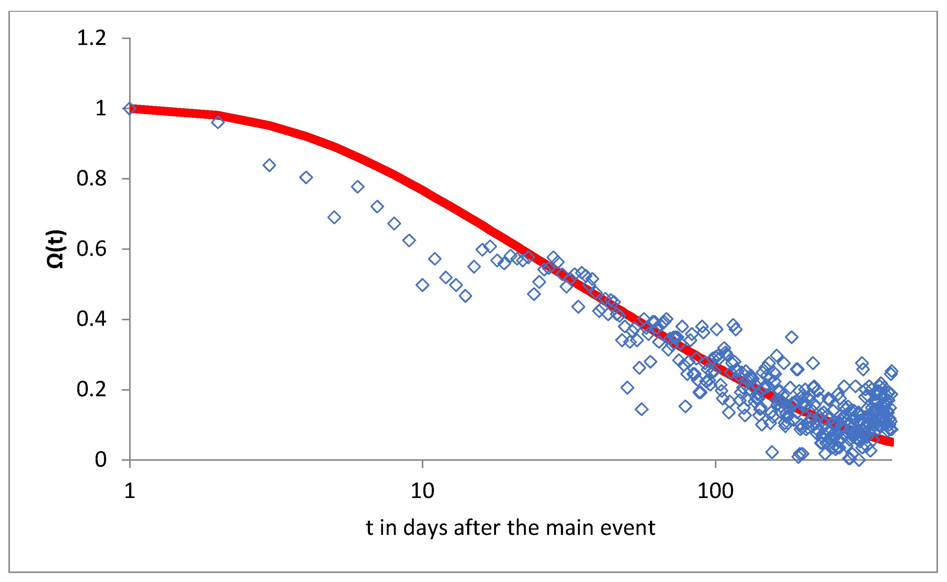
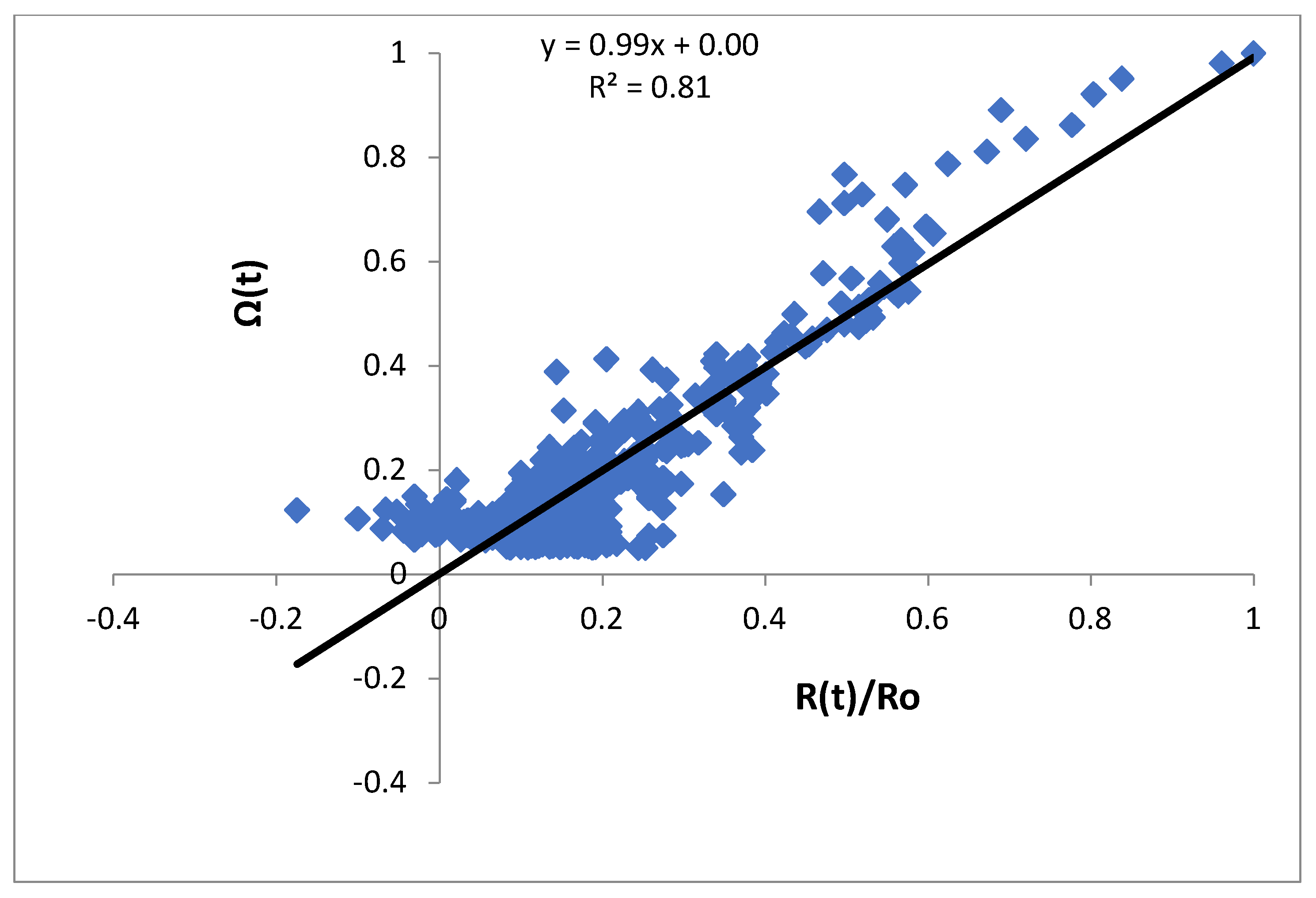
In Figure 6, the experimentally estimated Ω(t) function for the first 400 days of the post-seismic relaxation after the Lefkas main event is given, along with the calculated one using Equation (16) for τ_min ≈ 3.5 days and τ_max ≈ 350 days, respectively. A comparison of the observed and calculated values is given in Figure 7, along with a dichotomous line.

Furthermore, we note that ${\int }_0^{\infty }\Omega (t)dt=\frac{{\tau }_{max}-{\tau }_{min}}{R_o},$ which, after using the experimental values of Ω, leads to ${\tau }_{max} \approx 360$ days in quite good agreement with the value used in Figure 5 and Figure 6. We note that the law values of $\frac{R\left(t\right)}{R_o}$ in Figure 7 correspond to the logarithmic part of relaxation, while the high values are related with the part just after the rupture where the uncertainty in the estimated displacement is higher.

4. Discussion

Most of the models used to describe post-seismic relaxation are based on the assumption of a single relaxation time estimated for each relaxation mechanism proposed [4,11,14,60,61]. A co-seismic deformation leaves the system in a metastable state taking place in the broad earthquake zone. In the present work, the post-seismic relaxation is viewed as a superposition of several different relaxation times, each one activated in different mesoscopic domains of the macroscopic relaxed seismic volume. The macroscopic relaxation observed is a result of the superposition of different relaxation times on the microscopic–mesoscopic scale. This slow thermodynamic recovery could be explained by a physical model based on the Arrhenius Equation [62].

The lithosphere as a dynamical system under a post-seismic relaxation is a complex systems with strong interactions between its mesoscopic “subvolumes” [63] and, thus, could be viewed as a macroscopic system driven by hierarchically constrained dynamics [28] involved in the macroscopically observed relaxation process as a sequential series of correlated mesoscopic processes.

The view of hierarchical constrained dynamics could be a physical pathway to describe many of the complex systems that present logarithmic relaxation [64,65,66]. In the case of post-seismic phase, the applied tectonic load drives the system to fracture, and its relaxation creates a reorganization of the stress field in some selected mesoscopic regions of the system. The deformed subvolumes nearest to the fractured region are rearranged and the system reorganized. These new stress changes will affect the deformed subvolumes outside the area nearest to the fracture, permitting their relaxation, and so on. The above picture suggests that the relaxation in the fractured fault system is slow because it consists of a large number of correlated and strongly interacting reorganization steps with an increasing relaxation time. It seems to be appropriate to describe macroscopical post-seismic relaxation in terms of a lithosphere that presents a hierarchical pattern, with the faster relaxation to be associated with the subvolume close to earthquake focus regions and, due to strong correlations and long-range interactions, the slower relaxation time to be related with the “outer” deformed, but in the broad vicinity of epicenter, regions. The latter is in agreement with that proposed for complex relaxed systems with cluster interactions, where the relaxation time τ scales with the relaxation volume as τ~V^α, where α is an exponent related macroscopically with the fractal geometry of the subvolume distribution and the dynamical nature of relaxation [67,68,69]. This type of hierarchically constrained dynamics is able to derive the logarithmic relaxation frequently observed and associate it with thermally activated processes. We note that this behavior can result either from the parallel relaxation of subvolumes or by a sequential relaxation series of strongly correlated complex events [28].

Our results are in agreement with that presented in [70], where a Burridge-Knopoff (BK) model is used to describe the time dependence of the mean stress, assuming that a uniform statistical distribution of stress values is acting on each block (i.e., deformation in subvolumes) in the relaxing lithospheric system.

In [70], the post-seismic normalized stress relaxation of the strongly interacted elements of the BK model presents a stress relaxation that could be viewed as hierarchically constrained since blocks increase the stress on their nearby elements when they slip, and as a consequence, the probability that their neighbors will slip increases as well. They conclude that the normalized mean stress <σ> during the post-seismic relaxation in a BK model with a uniform distribution of stresses [71] is:

$$<\sigma >={{\displaystyle \int }}_0^1\sigma e^{-\nu t\exp (-\beta {\epsilon }_m\left(1-{\sigma }^2\right))}d\sigma$$

(17)

where ε_m is the maximum size of energy barrier, ν is an attempt frequency to jump over the energy barrier, and β = 1/k_BT. Approximation of (17) leads to the following behavior in short, intermediate, and long time periods, respectively:

$$\underset{t\to 0}{\lim }<\sigma >=\frac{1}{2}-\frac{1}{2\beta {\epsilon }_m}\left(1-\exp \left(-\beta {\epsilon }_m\right)\right)\nu t$$

(18)

$${<\sigma >}_{int}\approx \frac{1}{2}-\frac{1}{2\beta {\epsilon }_m}(\gamma +\ln \left(\nu t\right)$$

(19)

where γ is the Euler–Mascheroni constant (γ ≈ 0.577).

$$\underset{t\to \infty }{\lim }<\sigma >=\frac{\exp \left(\beta {\epsilon }_m\right)}{2\beta {\epsilon }_m}\frac{\exp (-\nu t\exp \left(-\beta {\epsilon }_m\right)}{\nu t}$$

(20)

which, for very long time periods, t is proportional to exp(−t/τ) with τ = exp(β${\epsilon }_m$)/ν.

A comparison of Equations (18)–(20) with Equation (10), (12), and (14), respectively, implies that $S ~\frac{1}{2\beta {\epsilon }_m}$, supporting the hypothesis that the scaling factor depends on temperature and the energy barrier that must be overcome before the relaxed subvolume moves to a new stress stage. In addition, ${\tau }_{max} ~\frac{1}{\nu }\exp \left(\beta {\epsilon }_m\right) \mathrm{and} {\tau }_{min} ~\frac{1}{\nu }$ with $\ln \left(\frac{{\tau }_{max}}{{\tau }_{min}}\right)~\beta {\epsilon }_m$ being an expression similar to that defined in the present approach using the Arrhenius expression, if ${\epsilon }_m=E_{max}-E_{min}$ is the maximum size of energy barrier.

The relaxation function, as presented in Equation (6), explains the logarithmic relaxation observed. In addition, it results in finite values, both just after the perturbation (i.e., t = 0) and for a long time after the earthquake event (t → ∞). The relaxation function R(t) can be explained by Arrhenius’ law, presenting a universal behavior of the relaxation process. Following Equation (6) and the ideas of hierarchically constrained dynamics, the faster relaxation mechanisms, related to small relaxed volumes (small τ), offer a more significant contribution to the relaxation process than the slower relaxation mechanisms (large τ related with the broader relaxed area), as indicated by the presence of term 1/τ in the expression of R(t), which permits greater weight to fast relaxation processes. We note that the superposition of relaxation mechanisms, as expressed in Equation (6), implies that, for early time periods, the fast relaxation mechanism associated with small relaxed volumes that have a relaxation time close to τ_min dominates, while for late time periods, the slow relaxation mechanism, related to the relaxation of volumes farther from the epicenter and present relaxation time close to τ_max, contributes most. It is reasonable to assume that the maximum relaxation time depends on the perturbation that triggers the relaxation and, thus, on the deformed volume related with the main event, along with the geotectonic conditions in the deformed region, such as stress, temperature, and fluids.

In addition, measurements of τ_min could give information on the fastest relaxation mechanism, which is scaled with the smallest deformed subvolume, even if it is sometimes not clearly observed due to the immediate transition of the deformation process into the logarithmic range, resulting in an unreliable estimation of τ_min.

Applying the generic hierarchically constrained dynamics view to the North–South displacement of the post-seismic relaxation of Lefkas 17 November 2015, Mw6.5 earthquake, we conclude that this approach describes with good agreement the displacement as estimated using cGNSS recordings during the post-seismic relaxation period, leading to the estimation of τ_min ≈ 3.5 days and τ_max ≈ 350 days, respectively.

This is a rather new approach that is used to describe post-seismic relaxation based on the assumption of a spectrum of relaxation times that are superposed, each of them activated in different mesoscopic domains of the macroscopic relaxed seismic volume. This slow thermodynamic recovery (i.e., a logarithmic time dependence) could be explained by a physical model based on the Arrhenius equation. With such an approach, we are led to finite values for t = 0, without assuming any empirical constitutional equation.

5. Concluding Remarks

In the present work the post-seismic relaxation is viewed as a superposition of several different relaxation times, each one activated in different mesoscopic domains of the macroscopic relaxed seismic volume. The macroscopic relaxation that is observed is a result of the superposition of different relaxation times on the microscopic–mesoscopic scale. This approach is a new one since most of the models used to describe post-seismic relaxation are based on the assumption of a single relaxation time estimated for each relaxation mechanism proposed. The slow thermodynamic recovery of the post-seismic relaxation could be explained by a physical model based on the Arrhenius equation and an appropriate distribution of relaxation times.

In summary, we can state that, in the present work:

• A multiscale post-seismic relaxation mechanism based on the existence of a distribution in relaxation time is presented.
• Assuming an Arrhenius dependence of the relaxation time with the uniform distributed activation energy in a mesoscopic scale, we conclude there is a generic logarithmic type relaxation on a macroscopic scale.
• The hierarchically constrained dynamics model could be used to understand the evolution of post seismic relaxation.
• The model was applied in the case of 2015 Lefkas (Greece) Mw6.5 earthquake, where cGNSS time series were recorded in a station located in the vicinity of the epicentral area. The application of the present approach to the Lefkas event fits the observed displacements, implying a distribution of relaxation times in the range τ_min ≈ 3.5 days to τ_max ≈ 350 days.

These results offer a stimulating finding for further studies that will investigate post-seismic deformation timeseries for other strong earthquakes, which may provide new insights into the underlying dynamics of earthquake relaxation processes, along with the possible parameters that influence this behaviour (i.e., fault type, local conditions, regional stress field, etc.).

References

- Hearn, E.H. What can GPS data tell us about the dynamics of post-seismic deformation? Geophys. J. Int. 2003, 155, 753–777. [Google Scholar] [CrossRef]
- Nur, A.; Byerlee, J.D. An effective stress law for elastic deformation of rocks with fluids. J. Geophys. Res. 1971, 76, 414–419. [Google Scholar] [CrossRef]
- Wang, H.F. Theory of Linear Poroelasticity with Applications to Geomechanics and Hydrogeology; Princeton University Press: Princeton, NJ, USA, 2000; Volume 2, p. 276. [Google Scholar]
- Marone, C.J.; Scholtz, C.H.; Bilham, R. On the mechanics of earthquake afterslip. J. Geophys. Res. 1991, 96, 8441–8452. [Google Scholar] [CrossRef]
- Pollitz, F.F.; Bürgmann, R.; Segall, P. Joint estimation of afterslip rate and postseismic relaxation following the 1989 Loma Prieta earthquake. J. Geophys. Res. 1998, 103, 26975–26992. [Google Scholar] [CrossRef] [Green Version]
- Montési, L.G.J. Controls of shear zone rheology and tectonic loading on postseismic creep. J. Geophys. Res. 2004, 109, B10404. [Google Scholar] [CrossRef] [Green Version]
- Marone, C.; Raleigh, C.B.; Scholz, C.H. Frictional behavior and constitutive modeling of simulated fault gouge. J. Geophys. Res. 1990, 95, 7007–7025. [Google Scholar] [CrossRef]
- Hetland, E.A.; Hager, B.H. The effects of rheological layering on post-seismic deformation. Geophys. J. Int. 2006, 166, 277–292. [Google Scholar] [CrossRef] [Green Version]
- Wang, L.; Hainzl, S.; Sinan Özeren, M.; Ben-Zion, Y. Postseismic deformation induced by brittle rock damage of aftershocks. J. Geophys. Res. 2010, 115, B10422. [Google Scholar] [CrossRef] [Green Version]
- Ingleby, T.; Wright, T.J. Omori-like decay of postseismic velocities following continental earthquakes. Geophys. Res. Lett. 2017, 44, 3119–3130. [Google Scholar] [CrossRef]
- Perfettini, H.; Avouac, J.-P. Postseismic relaxation driven by brittle creep: A possible mechanism to reconcile geodetic measurements and the decay rate of aftershocks, application to the Chi-Chi earthquake, Taiwan. J. Geophys. Res. 2004, 109. [Google Scholar] [CrossRef]
- Mallick, N.; Ciliberto, S.; Roux, S.G.; Di Stephano, P.; Vanel, L. Aftershocks in thermally activated rupture of indented glass. In Proceedings of the 12th International Conference on Fracture, ICF-12, Ottawa, ON, Canada, 12–17 July 2009; Volume 6, pp. 4564–4572. [Google Scholar]
- Bürgmann, R.; Segall, P.; Lisowski, M.; Svarc, J. Postseismic strain following the 1989 Loma Prieta earthquake from GPS and leveling measurements. J. Geophys. Res. 1997, 102, 4933–4955. [Google Scholar] [CrossRef] [Green Version]
- Yu, S.B.; Kuo, L.C.; Hsu, Y.J.; Su, H.H.; Liu, C.C.; Hou, C.; Lee, J.F.; Shin, T.C. Preseismic deformation and coseismic displacements associated with the 1999 Chi-Chi, Taiwan, earthquake. Bull. Seismol. Soc. Am. 2001, 91, 995–1012. [Google Scholar] [CrossRef]
- Hearn, E.H.; Bürgmann, R.; Reilinger, R.E. Dynamics of İzmit earthquake postseismic deformation and loading of the Düzce earthquake hypocenter. Bull. Seismol. Soc. Am. 2002, 92, 172–193. [Google Scholar] [CrossRef] [Green Version]
- Takahashi, H.; Nakao, S.; Okazaki, N.; Koyama, J.; Sagiya, T.; Ito, T.; Ohya, F.; Sato, K.; Fujita, Y.; Hashimoto, M.; et al. GPS observation of the first month of postseismic crustal deformation associated with the 2003 Tokachi-oki earthquake (MJMA 8.0), off southeastern Hokkaido. Earth Planets Space 2004, 56, 377–382. [Google Scholar] [CrossRef] [Green Version]
- Anugrah, B.; Meilano, I.; Gunawan, E.; Efendi, J. Estimation of postseismic deformation parameters from continuous GPS data in northern Sumatra after the 2004 Sumatra-Andaman earthquake. Earthq. Sci. 2015, 28, 347–352. [Google Scholar] [CrossRef] [Green Version]
- Tobita, M. Combined logarithmic and exponential function model for fitting postseismic GNSS time series after 2011 Tohoku-Oki earthquake. Earth Planets Space 2011, 68, 1–12. [Google Scholar] [CrossRef] [Green Version]
- Marone, C. Laboratory-derived friction laws and their application to seismic faulting. Annu. Rev. Earth Planet. Sci. 1998, 26, 643–696. [Google Scholar] [CrossRef] [Green Version]
- Kawada, Y.; Nagahama, H.; Hara, H. Irreversible thermodynamic and viscoelastic model for power-law relaxation and attenuation of rocks. Tectonophysics 2006, 427, 255–263. [Google Scholar] [CrossRef]
- Brantut, N.; Heap, M.; Baud, P.; Meredith, P. Mechanisms of time-dependent deformation in porous limestone. J. Geophys. Res. 2014, 119, 5444–5463. [Google Scholar] [CrossRef]
- Bocquet, L.; Charlaix, E.; Ciliberto, S.; Crassous, A. Moisture-induced ageing in granular media and the kinetics of capillary condensation. Nature 1998, 396, 735–737. [Google Scholar] [CrossRef]
- Renard, F.; Dysthe, D.; Feder, J.; Meakin, P.; Morris, S.; Jamtveit, B. Pattern formation during healing of fluid-filled cracks: An analog experiment. Geofluids 2009, 9, 365–372. [Google Scholar] [CrossRef]
- Ten Cate, J.A.; Shankland, T.J. Slow dynamics in the nonlinear elastic response of Berea sandstone. Geophys. Res. Lett. 1996, 21, 3019–3022. [Google Scholar] [CrossRef] [Green Version]
- Gibbs, M.; Evetts, J.; Leake, J. Activation energy spectra and relaxation in amorphous materials. J. Mater. Sci. 1983, 18, 278–288. [Google Scholar] [CrossRef]
- Shaknhovich, E.; Gutin, A. Relaxation to equilibrium in the random energy model. Eurphys. Lett. 1989, 9, 569–574. [Google Scholar] [CrossRef]
- Ten Cate, J.; Smith, E.; Guyer, R. Universal slow dynamics in granular solids. Phys. Rev. Lett. 2000, 85, 1020–1023. [Google Scholar] [CrossRef] [PubMed] [Green Version]
- Brey, J.; Prados, A. Slow logarithmic relaxation in models with hierarchically constrained dynamics. Phys. Rev. E 2001, 63, 21108. [Google Scholar] [CrossRef] [PubMed] [Green Version]
- Amir, A.; Oreg, Y.; Imry, Y. On relaxations and aging of various glasses. Proc. Natl. Acad. Sci. USA 2012, 109, 1850–1855. [Google Scholar] [CrossRef] [PubMed] [Green Version]
- Zaitsev, V.; Gusev, V.; Tournat, V.; Richard, P. Slow relaxation and aging phenomena at the nanoscale in granular materials. Phys. Rev. Lett. 2014, 112, 108302. [Google Scholar] [CrossRef] [Green Version]
- Varotsos, P.; Alexopoulos, C. Thermodynamics of Point Defects and Their Relation with the Bulk Properties; Amelinckx, S., Gevers, R., Nihoul, J., Eds.; Elsevier: Amsterdam, The Netherlands, 1986. [Google Scholar]
- Ganas, A.; Drakatos, G.; Rontogianni, S.; Tsimi, C.; Petrou, P.; Papanikolaou, M.; Argyrakis, P.; Boukouras, K.; Melis, N.; Stavrakakis, G. NOANET: The new permanent GPS network for Geodynamics in Greece. Geophys. Res. Abstr. 2008, 10, EGU2008–A–04380. [Google Scholar]
- Snieder, R.; Sens-Schönfelder, C.; Wu, R. The time dependence of rock healing as a universal relaxation process, a tutorial. Geophys. J. Int. 2017, 208, 1–9. [Google Scholar] [CrossRef] [Green Version]
- Ranalli, G. Rheology of the Earth; Allen and Unwin Inc.: Winchester, MA, USA, 1987. [Google Scholar]
- Ergintav, S.; Bürgmann, R.; McClusky, S.; Çakmak, R.; Reilinger, R.E.; Lenk, O.; Barka, A.; Özener, H. Postseismic deformation near the İzmit earthquake (17 August 1999, M 7.5) rupture zone. Bull. Seismol. Soc. Am. 2002, 92, 194–207. [Google Scholar] [CrossRef]
- Pollitz, F.F. Transient rheology of the uppermost mantle beneath the Mojave Desert, California. Earth Planet. Sci. Lett. 2003, 215, 89–104. [Google Scholar] [CrossRef]
- Pollitz, F.F. Transient rheology of the upper mantle beneath central Alaska inferred from the crustal velocity field following the 2002 Denali earthquake. J. Geophys. Res. 2005, 110. [Google Scholar] [CrossRef] [Green Version]
- Abramowitz, M.; Stegun, I.A. Handbook of Mathematical Functions: With Formulas, Graphs, and Mathematical Tables; Dover Books on Mathematics: Dover, NY, USA, 1965. [Google Scholar]
- Papazachos, B.C. Seismicity of the Aegean and surrounding area. Tectonophysics 1009, 178, 287–308. [Google Scholar]
- Louvari, E.; Kiratzi, A.A.; Papazachos, B.C. The Cephalonia transform fault and its extension to western Lefkada island (Greece). Tectonophysics 1999, 308, 223–236. [Google Scholar] [CrossRef]
- Le Pichon, X.; Chamot Rooke, N.; Lallemant, S.; Noomen, R.; Veis, G. Geodetic determination of the kinematics of central Greece with respect to Europe: Implications for eastern Mediterranean tectonics. J. Geophys. Res. 1995, 100, 12675–12690. [Google Scholar] [CrossRef]
- Kokinou, E.; Papadimitriou, E.; Karakostas, V.; Kamberis, E.; Vallianatos, F. The Kefalonia Transform Zone (offshore Western Greece) with special emphasis to its prolongation towards the Ionian Abyssal Plain. Mar. Geophys. Res. 2006, 27, 241–252. [Google Scholar] [CrossRef]
- Van Hinsbergen, D.J.J.; van der Meer, D.G.; Zachariasse, W.J.; Meulenkamp, J.E. Deformation of western Greece during Neogene clockwise rotation and collision with Apulia. Int. J. Earth Sci. 2006, 95, 463–490. [Google Scholar] [CrossRef]
- Vassilakis, E.; Royden, L.; Papanikolaou, D. Kinematic links between subduction along the Hellenic trench and extension in the Gulf of Corinth, Greece: A multidisciplinary analysis. Earth Planet. Sci. Lett. 2011, 303, 108–120. [Google Scholar] [CrossRef]
- Lekkas, E.; Mavroulis, S.; Carydis, P.; Alexoudi, V. The 17 November 2015 Mw 6.4 Lefkas (Ionian Sea, Western Greece) Earthquake: Impact on Environment and Buildings. Geotech. Geol. Eng. 2018, 36, 2109–2142. [Google Scholar] [CrossRef]
- Karastathis, V.; Mouzakiotis, E.; Ganas, A.; Papadopoulos, G.A. High-precision relocation of seismic sequences above a dipping Moho: The case of the January–February 2014 seismic sequence on Cephalonia island (Greece). Solid Earth 2015, 6, 173–184. [Google Scholar] [CrossRef] [Green Version]
- Karakostas, V.; Papadimitriou, E.; Papazachos, C.B. Properties of the 2003 Lefkada, Ionian Islands, Greece, earthquake seismic sequence and seismicity triggering. Bull. Seismol. Soc. Am. 2004, 94, 1976–1981. [Google Scholar] [CrossRef] [Green Version]
- Papadimitriou, P.; Kaviris, G.; Makropoulos, K. The Mw = 6.3 2003 Lefkada Earthquake (Greece) and induced stress transfer changes. Tectonophysics 2006, 423, 73–82. [Google Scholar] [CrossRef]
- Lagios, E.; Sakkas, V.; Papadimitriou, P.; Damiata, B.N.; Parcharidis, I.; Chousianitis, K.; Vassilopoulou, S. Crustal deformation in the Central Ionian Islands (Greece): Results from DGPS and DInSAR analyses (1995–2006). Tectonophysics 2007, 444, 119–145. [Google Scholar] [CrossRef]
- Saltogianni, V.; Stiros, S. A two-fault model of the 2003 Leucas (Aegean Arc) earthquake based on topological inversion of GPS data. Bull. Seismol. Soc. Am. 2015, 105, 2510–2520. [Google Scholar] [CrossRef]
- Papadopoulos, G.A.; Karastathis, V.; Koukouvelas, I. The Cephalonia, Ionian Sea (Greece), sequence of strong earthquakes of January-February (2014): A first report. Res. Geophys. 2015, 4, 5441. [Google Scholar] [CrossRef] [Green Version]
- Karakostas, V.; Papadimitriou, E.; Mesimeri, M.; Gkarlaouni, C.; Paradisopoulou, P. The 2014 Kefalonia doublet (Mw6.1 and Mw6.0) central Ionian Islands, Greece: Seismotectonic implications along the Kefalonia transform fault zone. Acta Geophys. 2015, 63, 1–16. [Google Scholar] [CrossRef] [Green Version]
- Chousianitis, K.; Konca, A.O.; Tselentis, G.-A.; Papadopoulos, G.A.; Gianniou, M. Slip model of the 17 November 2015 M=6.5 Lefkada earthquake from the joint inversion of geodetic and seismic data. Geophys. Res. Lett. 2016, 43, 7973–7981. [Google Scholar] [CrossRef] [Green Version]
- Papadimitriou, E.; Karakostas, V.; Mesimeri, M.; Chouliaras, G.; Kourouklas, C. The Mw6.5 17 November 2015 Lefkada (Greece) Earthquake: Structural Interpretation by Means of the Aftershock Analysis. Pure Appl. Geophys. 2017, 174, 3869–3888. [Google Scholar] [CrossRef]
- Bernese GNSS Software Version 5.2. User Manual; Dach, R.; Lutz, S.; Walser, P.; Fridez, P. (Eds.) Astronomical Institute, University of Bern; Bern Open Publishing: Bern, Switzerland, 2015; ISBN 978-3-906813-05-9. [Google Scholar] [CrossRef]
- Niell, A.E. Global mapping functions for the atmosphere delay at radio wavelengths. J. Geophys. Res. 1996, 101, 3227–3246. [Google Scholar] [CrossRef]
- Saastamoinen, I.I. Contribution to the theory of atmospheric refraction. Bull. Géodésique 1972, 105, 279–298. [Google Scholar] [CrossRef]
- Ray, R.D.; Ponte, R.M. Barometric tides from ECMWF operational analyses. Ann. Geophys. 2003, 21, 1897–1910. [Google Scholar] [CrossRef] [Green Version]
- Tsallis, C. Some open points in nonextensive statistical mechanics. Int. J. Bifurc. Chaos 2012, 22, 1230030. [Google Scholar] [CrossRef] [Green Version]
- Savage, J.C.; Svarc, J.L. Post seismic deformation associated with the 1992 Mw = 7.3 Landers earthquake, southern California. J. Geophys. Res. 1997, 102, 7565–7577. [Google Scholar] [CrossRef]
- Savage, J.; Svarc, J.; Yu, S.-B. Postseismic relaxation and transient creep. J. Geophys. Res. 2005, 110, B11402. [Google Scholar] [CrossRef]
- Ten Cate, J. Slow dynamics of earth materials: An experimental overview. Pure Appl. Geophys. 2011, 168, 2211–2219. [Google Scholar] [CrossRef]
- Vallianatos, F.; Chatzopoulos, G. A Complexity View into the Physics of the Accelerating Seismic Release Hypothesis: Theoretical Principles. Entropy 2018, 20, 754. [Google Scholar] [CrossRef] [PubMed] [Green Version]
- Tarasov, A.; Titov, K. Relaxation time distribution from time domain induced polarization measurements. Geophys. J. Int. 2007, 170, 31–43. [Google Scholar] [CrossRef] [Green Version]
- Zaitsev, V.; Gusev, V.; Castagnede, B. Thermoelastic mechanism for logarithmic slow dynamics and memory in elastic wave interactions with individual cracks. Phys. Rev. Lett. 2003, 90, 75501. [Google Scholar] [CrossRef] [PubMed] [Green Version]
- Ostrovsky, L.; Lebedev, A.; Riviere, J.; Shokouhi, P.; Wu, C.; Stuber Geesey, M.A.; Johnson, P.A. Long-Time Relaxation Induced by Dynamic Forcing in Geomaterials. J. Geophys. Res. 2019, 124, 5003–5013. [Google Scholar] [CrossRef]
- Brouers, F.; Sotolongo-Costa, O. Universal relaxation in nonextensive systems. Eurphys. Lett. 2003, 62, 808–814. [Google Scholar] [CrossRef] [Green Version]
- Brouers, F.; Sotolongo-Costa, O. Relaxation in heterogeneous systems: A rare events dominated phenomenon. Phys. A Stat. Mech. Appl. 2005, 356, 359–374. [Google Scholar] [CrossRef]
- Vallianatos, F. On the non-extensive nature of the Isothermal Depolarization relaxation Currents in cement mortars. J. Phys. Chem. Solid 2012, 73, 550–553. [Google Scholar] [CrossRef]
- Huisman, B.; Fasolino, A. Logarithmic relaxation due to minimization of interactions in the Burridge-Knopoff model. Phys. Rev. E 2006, 74, 26110. [Google Scholar] [CrossRef] [PubMed] [Green Version]
- Persson, B.N.J. Theory of friction: Stress domains, relaxation and creep. Phys. Rev. B 1995, 51, 13568–13585. [Google Scholar] [CrossRef] [PubMed]
Figure 1.
Example of exponential relaxation (see Equation (1)) with S = 5 mm, u∞ = −25 mm and τ = 300 days.
Figure 2.
The relaxation function R(t) (see Equation (6) in the text) for τmin = 5 days and τmax = 200, 400, 600 days.
Figure 3.
Map of the central Ionian islands of Lefkas, Cephalonia, and Ithaca, showing the main faulting zones and marking the continuous GNSS stations (triangles) PONT and SPAN in Lefkas and VLSM in Cephalonia islands. Circles represent the earthquake epicenters (M > 3) after the 17 November 2015 main event. Red and blue vectors represent the cGNSS horizontal velocities before and after the 2015 earthquake, respectively. Black arrows show the co-seismic deformation. CTF: Cephalonia Transform Fault.
Figure 4.
Time series of PONT continuous GNSS stations located in Lefkas island. Red line indicates the date of the 2015 seismic event.
Figure 5.
The observed displacement, along with the theoretical calculated using Equation (1) (see text), with S = 4.8 mm, , τmin ≈ 3.5 days, and τmax ≈ 350 days (i.e., Ro ≈ 4.6) is presented as a very good agreement.
Figure 6.
The experimentally estimated Ω(t) function for the first 400 days of the post-seismic relaxation after the Lefkas main event, along with the calculated one using Equation (16) for τmin ≈ 3.5 days and τmax ≈ 350 days, respectively.
Figure 7.
A comparison of the experimentally estimated Ω(t) function with the calculated values R(t)/Ro for the post-seismic relaxation period after the Lefkas main event for τmin ≈ 3.5 days and τmax ≈ 350 days, respectively (see text).
Publisher’s Note: MDPI stays neutral with regard to jurisdictional claims in published maps and institutional affiliations. |
© 2021 by the authors. Licensee MDPI, Basel, Switzerland. This article is an open access article distributed under the terms and conditions of the Creative Commons Attribution (CC BY) license (https://creativecommons.org/licenses/by/4.0/).
Share and Cite
MDPI and ACS Style
Vallianatos, F.; Sakkas, V. Multiscale Post-Seismic Deformation Based on cGNSS Time Series Following the 2015 Lefkas (W. Greece) Mw6.5 Earthquake. Appl. Sci. 2021, 11, 4817. https://doi.org/10.3390/app11114817
AMA Style
Vallianatos F, Sakkas V. Multiscale Post-Seismic Deformation Based on cGNSS Time Series Following the 2015 Lefkas (W. Greece) Mw6.5 Earthquake. Applied Sciences. 2021; 11(11):4817. https://doi.org/10.3390/app11114817
Chicago/Turabian StyleVallianatos, Filippos, and Vassilis Sakkas. 2021. "Multiscale Post-Seismic Deformation Based on cGNSS Time Series Following the 2015 Lefkas (W. Greece) Mw6.5 Earthquake" Applied Sciences 11, no. 11: 4817. https://doi.org/10.3390/app11114817
Note that from the first issue of 2016, this journal uses article numbers instead of page numbers. See further details here.