Niching Grey Wolf Optimizer for Multimodal Optimization Problems

Abstract

Metaheuristic algorithms are widely used for optimization in both research and the industrial community for simplicity, flexibility, and robustness. However, multi-modal optimization is a difficult task, even for metaheuristic algorithms. Two important issues that need to be handled for solving multi-modal problems are (a) to categorize multiple local/global optima and (b) to uphold these optima till the ending. Besides, a robust local search ability is also a prerequisite to reach the exact global optima. Grey Wolf Optimizer (GWO) is a recently developed nature-inspired metaheuristic algorithm that requires less parameter tuning. However, the GWO suffers from premature convergence and fails to maintain the balance between exploration and exploitation for solving multi-modal problems. This study proposes a niching GWO (NGWO) that incorporates personal best features of PSO and a local search technique to address these issues. The proposed algorithm has been tested for 23 benchmark functions and three engineering cases. The NGWO outperformed all other considered algorithms in most of the test functions compared to state-of-the-art metaheuristics such as PSO, GSA, GWO, Jaya and two improved variants of GWO, and niching CSA. Statistical analysis and Friedman tests have been conducted to compare the performance of these algorithms thoroughly.

1. Introduction

The area of nature-inspired metaheuristic algorithms is continuously evolving with newly developed algorithms. These algorithms are well known for their widespread local and global search ability, local optima avoidance, and quick convergence ability. In addition, these algorithms do not need any knowledge of a function’s gradient or differentiability [1,2]. Since the metaheuristic algorithms have these superior properties with easy applicability and fewer parameter requirements, significant variants of these algorithms are developed [3]. The most widely used algorithms are Simulated Annealing (SA) [4], Genetic Algorithm (GA) [5], Particle Swarm Optimization (PSO) [6], Differential Evolution (DE) [7], and Ant Colony Optimization (ACO) [8]. A few recent metaheuristics that seek the attention of researchers is Bee Collecting Pollen Algorithm (BCPA) [9], Black Hole (BH) [10] Algorithm, Artificial Bee Colony Algorithm (ABC) [11], Central Force Optimization (CFO) [10], Electro-search Algorithm (ESA) [12], Gravitational Search Algorithm (GSA) [13], Teaching Learning Based Algorithm (TLBO) [14], Artificial Chemical Reaction Optimization Algorithm (ACROA) [15], Firefly Algorithm (FA) [16], Big Bang–Big Crunch (BBBC) [17], Grey Wolf Optimizer (GWO) [18], Dragon Fly Algorithm [19], and Harris Hawk Optimizer (HHO) [20], Jaya Algorithm [21]. Among these recent metaheuristics, the GSA, GWO, and Jaya Algorithm is well known for simplicity, effective exploration and exploitation.

Among the algorithms mentioned above, the GWO is a novel metaheuristic algorithm that falls under swarm intelligence [18]. This algorithm has been proposed mimicking the organizational order of wolves and their collective hunting nature. Due to its simplicity, fast seeking speed, good precision for search, and fewer controlling parameters, this algorithm is successfully applied to various technical fields such as feature selection [22,23,24], wind speed forecasting [25], optimal power flow [26,27], pattern recognition [28], unit commitment [29,30] parameters estimation [31,32], wellbore trajectory optimization [31]. In addition to these applications, the GWO and variants also performed well for combinatorial optimization problems and successfully applied to different fields, such as vehicle routing problem [32], job scheduling problems [33,34,35], and economic dispatch [36,37] problems. Some modifications to the GWO algorithm and its application in various optimization fields are now described.

Quasi-oppositional based learning (Q-OBL) GWO called QOGWO was proposed by Guha et al. [38] to control power systems load frequency. The authors designed optimal PID controller by using QOGWO for two areas and four hydrothermal power plants and showed that their proposed methods achieved promising performance like fuzzy logic, ANN, and ANFIS system. In a different research, crossover and mutation-based hybrid GWO was proposed by Jayabarathi et al. [36] to optimize non-linear, non-convex, constrained, and unconstrained economic dispatch problems at different conditions. The authors claimed that their method showed promising performance. Korayem et al. hybridized the GWO with K-means clustering technique to solve CVRP (capacitated vehicle routing problems) and named it as K-GWO [32]. The authors further integrated a capacity constraint to their algorithm and proposed 2 clustering techniques. They follow the cluster-first route-second method to solve CVRP problems and tested their proposed technique for 20 benchmarks, and the obtained solutions are within a mean deviation of 1.76% from the known optimum solutions. Singh and Singh [39] proposed a hybridization of GWO with SCA in 2017. The hybrid GWOSCA shows good performance for unimodal functions but failed to perform better for multi-modal problems [39]. Jiang and zhang applied a hybrid Grey Wolf Optimizer algorithm for job shop scheduling and flexible job shop scheduling problems. Their hybrid algorithm is incorporated with crossover operator to handle discrete variables, whereas mutation operator helps to avoid local optima, and a neighborhood search is applied to increase exploration. Their proposed algorithm outperforms PAGA, LSGA, TLBO, EDA, BFO algorithms for both case studies [40]. Long et al. [41] recommnded exploration-enhanced GWO (EEGWO), in which they introduced a new formula for updating the position by selecting a random wolf to guide the search and non-linearly controlling the GWO parameter “a”. Even after making these modifications, their proposed algorithm still suffers from premature convergence and local optima. Dhargupta et al. [42] designed the selective opposition-based learning GWO (SOGWO) to improve GWO’s convergence ability. To govern the omega wolves, they used Spearman’s correlation coefficient and chose a few dimensions of wolves to apply opposition, which enhanced the exploration ability of the algorithm. A recent variation of the GWO is developed by Shahraki et al. [43], where they suggested a new movement technique encouraged by the discrete hunting nature of wolves called dimension learning-based hunting (DLH) search. According to the DLH, all wolves create their neighbors, sharing information among themselves.

The literature mentioned above indicates that due to easy implementation and less parameter tuning, GWO variants are already applied in every optimization field and have shown good performances empirically. However, premature convergence and the inability to balance the exploitation with exploration are still the main drawbacks of the GWO and its variants for solving complex multi-modal optimization problems [42,43]. To overcome these limitations, we make a decent attempt to improve the GWO algorithm by adapting the niching technique. Niching techniques are well known to trace multiple optimal solutions together. These techniques increase population diversity and reduce the likelihood of being trapped in local solutions. In one iteration, they are also able to trace numerous local/global optima. A few standard niching techniques developed in recent years are clustering [44], fitness sharing [44], crowding [45], and clearing [46]. Nevertheless, niching methods need more function evaluations to reach the global optima. It has been seen from literature that various niching methods are applied to different types of metaheuristic algorithms such as GA [44,45,46], PSO [2,47,48,49], CSA [50], and niching technique has significantly improved the performance of these optimization algorithms. Inspired by these results, we incorporate a fitness Euclidean distance ratio (FER) based niching technique with modified velocity update and local search into the GWO algorithm, which has shown to significantly improve the basic GWO algorithm’s accuracy. Our proposed method also does not need any tuning parameters, which is a significant advantage. The research’s key contribution is to a) integrate FER niching technique into the GWO algorithm, b) modify the velocity update equation, and c) apply a local search technique at the end of the search process. To the best of our knowledge, this study first incorporates the niching technique to the GWO algorithm. Since the multi-modal function optimization also needs to allocate the desired global optima more precisely, we further incorporated the personal best feature of PSO to hold the good solutions. The remaining part of the article is organized as follows: Section 2 describes the NGWO algorithm. Section 3 illustrates the results and engineering applications of NGWO. Finally, Section 4 presents the conclusion.

2. Materials and Methods

2.1. Grey Wolf Optimizer

Mirjalili et al. [18] suggested GWO, a novel population-based algorithm, which falls under the swarm intelligence category. The key feature of GWO that makes it less prone to local solutions and better than other algorithms is that it searches for the best solutions by following three leader wolves: alpha, beta, and delta, while most other algorithms only follow one best solution. The common wolves are called omega, and they always follow the three leaders. The major steps of GWO are:

• Tracking, chasing, proceeding towards the target;
• Chasing, encompassing, distressing the target;
• Attacking the target.

The encircling mechanism can be mathematically represented as:

$${\overrightarrow{\mathrm{X}}}_{\left(\mathrm{k}+1\right)}={\overrightarrow{\mathrm{X}}}_{\mathrm{P}\left(\mathrm{k}\right)}-\overrightarrow{\mathrm{A}}.\left|\overrightarrow{\mathrm{C}}.{\overrightarrow{\mathrm{X}}}_{\mathrm{P}\left(\mathrm{k}\right)}-{\overrightarrow{\mathrm{X}}}_{\left(\mathrm{k}\right)}\right|$$

(1)

Here, vector $\overrightarrow{\mathrm{X}}$ indicates the position of wolves, $\overrightarrow{{\mathrm{X}}_{\mathrm{p}}}$ represents optimal solution’s position, $\overrightarrow{\mathrm{C}}$ and $\overrightarrow{\mathrm{A}}$ are acceleration coefficients, $\overrightarrow{\mathrm{C}}=2.\overrightarrow{{\mathrm{r}}_2}$ and $\overrightarrow{\mathrm{A}}=2\overrightarrow{\mathrm{a}}.\overrightarrow{{\mathrm{r}}_1}-\overrightarrow{\mathrm{a}}$, where $\overrightarrow{{\mathrm{r}}_1},$ and $\overrightarrow{{\mathrm{r}}_2}$ are randomly generated vectors within [0,1]. $\overrightarrow{\mathrm{a}}$ is a constant vector that declines linearly from 2 to 0. All the wolves update their positions by following these equations.

$${\overrightarrow{\mathrm{X}}}_{\left(\mathrm{a}\right)}={\overrightarrow{\mathrm{X}}}_{\mathsf{\alpha }}-\overrightarrow{\mathrm{A}}.\left|\overrightarrow{{\mathrm{C}}_1}.{\overrightarrow{\mathrm{X}}}_{\mathsf{\alpha }}-{\overrightarrow{\mathrm{X}}}_{}\right|$$

(2)

$${\overrightarrow{\mathrm{X}}}_{\left(\mathrm{b}\right)}=\overrightarrow{\mathrm{X}}\mathsf{\beta }-\overrightarrow{\mathrm{A}}.\left|\overrightarrow{{\mathrm{C}}_2}.\overrightarrow{\mathrm{X}}\mathsf{\beta }-{\overrightarrow{\mathrm{X}}}_{}\right|$$

(3)

$${\overrightarrow{\mathrm{X}}}_{\left(\mathrm{c}\right)}={\overrightarrow{\mathrm{X}}}_{\mathsf{\delta }}-\overrightarrow{\mathrm{A}}.\left|\overrightarrow{{\mathrm{C}}_3}.{\overrightarrow{\mathrm{X}}}_{\mathsf{\delta }}-{\overrightarrow{\mathrm{X}}}_{}\right|$$

(4)

$${\overrightarrow{\mathrm{X}}}_{}=\frac{\left({\overrightarrow{\mathrm{X}}}_{\left(\mathrm{a}\right)}+{\overrightarrow{\mathrm{X}}}_{\left(\mathrm{b}\right)}+{\overrightarrow{\mathrm{X}}}_{\left(\mathrm{c}\right)}\right)}{3}$$

(5)

At each iteration, the wolves will update their positions according to Equations (1)–(5). The parameter $\overrightarrow{\mathrm{a}}$ controls the movement of the wolves during the first half of the iteration period where $\overrightarrow{\mathrm{a}}$ > 1, and it will intensify the exploration ability of the algorithm. In the last half of the iteration period where $\overrightarrow{\mathrm{a}}$ < 1, it will increase the wolves’ exploitation ability.

2.2. Niching Technique

Niching techniques have the superiority of containing multiple solutions, which help them to handle the multi-modal functions and effectively reach the global optimal basin. In the proposed technique, the fitness Euclidean-distance ratio GWO (FER-GWO) is employed to locate the best closest solutions, and the FER-GWO is developed following the concept of FDR-PSO [51]. To calculate the FER value between two wolves i and j, the following equation has been utilized.

$${\mathrm{FER}}_{\mathrm{ij}}=\left(\mathsf{\alpha }\right).\frac{\mathrm{F}\left({\mathrm{p}}_{\mathrm{i}}\right)-\mathrm{F}\left({\mathrm{p}}_{\mathrm{j}}\right)}{\left|\left|{\mathrm{p}}_{\mathrm{i}}-{\mathrm{p}}_{\mathrm{j}}\right|\right|}$$

(6)

Here, p_i and p_j are the positions of the corresponding i and j wolves, and F(p_i) and F(p_j) represent their cost function values.

$$\mathrm{The}\mathrm{scaling}\mathrm{factor}\left(\mathsf{\alpha }\right)=\frac{\left|\left|\mathrm{S}\right|\right|}{\mathrm{F}\left({\mathrm{p}}_{\mathrm{b}}\right)-\mathrm{F}\left({\mathrm{p}}_{\mathrm{w}}\right)}$$

(7)

In the above equation F(p_w) and F(p_b) are the cost function values of the worst and best wolves among the current population, and the search space size is calculated based on decision variables bounds, and numerically represented as:

$$\mathrm{S}=\sqrt{{\displaystyle \sum }_{\mathrm{n}=1}^{\mathrm{D}}({\mathrm{x}}_{\mathrm{n}}^{\mathrm{u}}-{\mathrm{x}}_{\mathrm{n}}^{\mathrm{l}})^2}$$

(8)

Since, multi-modal optimization needs extensive exploration, niching is an efficient technique that could meet the requirement. Therefore, in the proposed GWO algorithm, we incorporated the personal best features to keep track of the best solutions discovered so far during the search process. The wolves will be guided towards more fittest neighborhood points at each iteration that can be obtained by calculating the FER values. The FER value has superiority in that it does not need parameters specification. Moreover, bigger population size is recommended for niching to locate all the local and global optima.

2.3. Modified Velocity Update Equation

During the iteration period, we determine the nbest_i of each wolf based on the FER value from Equation (6). The nbest_i value is further used to modify the velocity update Equation of beta and delta wolves, which is formulated as:

$${\overrightarrow{\mathrm{X}}}_{\left(\mathrm{b}\right)}=\overrightarrow{{\mathrm{nbest}}_{\mathrm{i}}}-\overrightarrow{\mathrm{A}}.\left|\overrightarrow{\mathrm{C}}.{\overrightarrow{\mathrm{nbest}}}_{\mathrm{i}}-\overrightarrow{\mathrm{X}}\right|$$

(9)

$${\overrightarrow{\mathrm{X}}}_{\left(\mathrm{c}\right)}=\overrightarrow{{\mathrm{nbest}}_{\mathrm{i}}}-\overrightarrow{\mathrm{A}}.\left|\overrightarrow{\mathrm{C}}.\overrightarrow{{\mathrm{nbest}}_{\mathrm{i}}}-{\overrightarrow{\mathrm{X}}}_{}\right|$$

(10)

We set a niching constant (NC) as 0.5 and generate a random number (r_i) during each iteration, if ri > NC, then the beta and delta wolves will be guided by nbest_i using Equations (9) and (10). Otherwise, the original Equations (3) and (4) will be used to guide the beta and delta wolves. Please note that the alpha wolf is always guided by the original position update equation (Equation (2)).

2.4. Local Search

It is challenging for the niching techniques to hit the global optima accurately in complex multi-modal problems reliably. We incorporated a local search technique into our NGWO to generate offspring close to the personal best (Pbest). It also improves the algorithm’s fine search capability, which increases the likelihood of obtaining optimal results. The definition of Qu et al. [2] is used to establish the local search technique, and the pseudo-code is provided below in Algorithm 1.

Algorithm 1 Local Search

1: Update the present Pbest by NGWO 2: for i = 1 to NP (number of wolves) 3:  Search Pbest_nearesti (the nearest Pbest member to Pbesti) 4:  if fit(Pbest_nearesti) < = fit(Pbesti) 5:   Temp = Pbesti + 1.5 * rand * (Pbest_nearesti–Pbesti) 6:  else 7:   Temp = Pbesti + 1.5 * rand * (Pbesti–Pbest_nearesti) 8:  end if 9:  Check for bounds violation, and assess Temp. 10:  if fit(Temp) < fit(Pbesti) 11:   Pbesti = Temp 12:  end if 13: end for

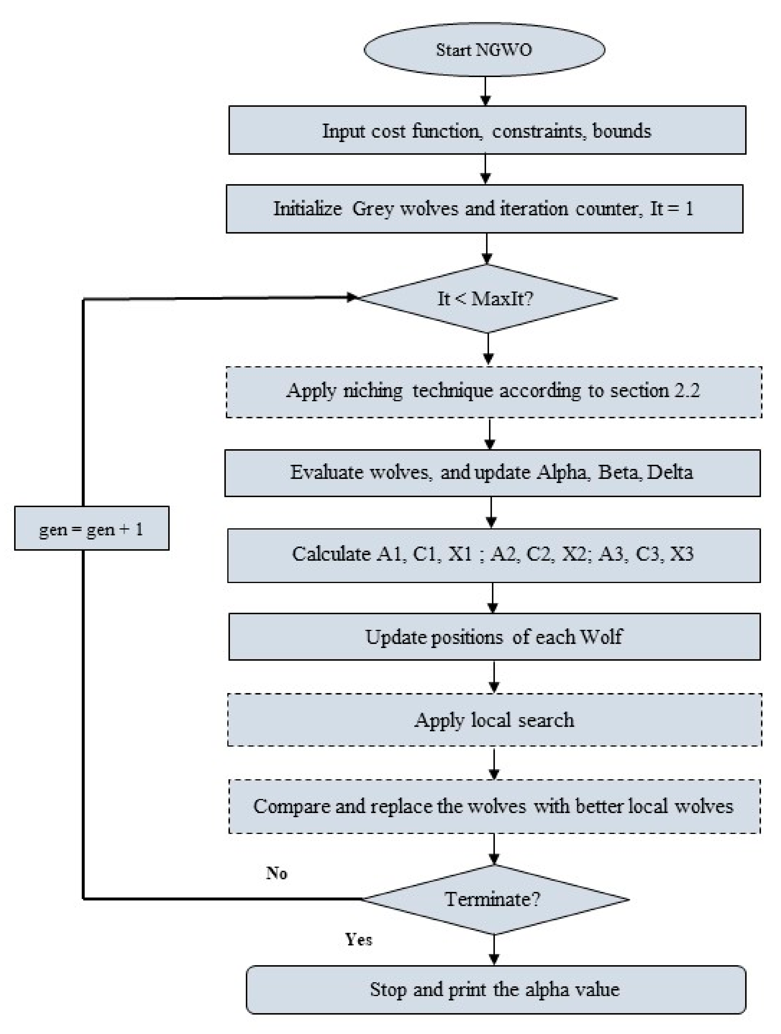
During each iteration of the NGWO, the niching technique is applied by using Equations (6)–(8). The wolves update their positions based on Equations (2)–(5) and (9)–(10). Finally, local search is applied to the wolves’ personal best (Pbest). Figure 1 shows a detailed flow map of the proposed algorithm.

3. Result and Discussion

3.1. Experimental Setup

We evaluated the proposed algorithm’s performance comprehensively for 23 test functions as a minimization problem [13,18]. These functions are very common for testing any algorithm’s effectiveness, consisting of 7 unimodal, 6 multi-modal, and 10 fixed dimensional multi-modal functions. The population and iteration number are set as 50 and 1000 for the proposed method, respectively. We keep these two features similar to the other compared studies to make the comparison fair and non-biased. The compared PSO, GSA, GWO, and SOGWO values are taken from [42], and niching CSA values are inserted from [50]. The Matlab code of Jaya algorithm and IGWO algorithms are collected from the authors website for comparison. The test functions are numerically presented here, and their detailed properties are described in

Table 1. Benchmark function properties.

Functions	Dimension	Range	Global Optima
F1	30	[−100, 100]	0
F2	30	[−10, 10]	0
F3	30	[−100, 100]	0
F4	30	[−100, 100]	0
F5	30	[−30, 30]	0
F6	30	[−100, 100]	0
F7	30	[−1.28, 1.28]	0
F8	30	[−500, 500]	−418 × D
F9	30	[−5.12, 5.12]	0
F10	30	[−32, 32]	0
F11	30	[−600, 600]	0
F12	30	[−50, 50]	0
F13	30	[−50, 50]	0
F14	2	[−65, 65]	1
F15	4	[−5, 5]	0.0003
F16	2	[−5, 5]	−1.0316
F17	2	[−5, 5]	0.398
F18	2	[−2, 2]	3
F19	3	[0, 1]	−3.86
F20	6	[0, 10]	−3.32
F21	4	[0, 10]	−10.1532
F22	4	[0, 10]	−10.4028
F23	4	[0, 10]	−10.5363

.

$${\mathrm{F}}_1\left(\mathrm{y}\right)={\displaystyle \sum }_{\mathrm{j}=1}^{\mathrm{D}}{\mathrm{y}}_{\mathrm{j}}^2$$

(11)

$${\mathrm{F}}_2\left(\mathrm{y}\right)={\displaystyle \sum }_{\mathrm{j}=1}^{\mathrm{D}}|{\mathrm{y}}_{\mathrm{j}}|+{\displaystyle \prod }_{\mathrm{j}=1}^{\mathrm{D}}\left|{\mathrm{y}}_{\mathrm{j}}\right|$$

(12)

$${\mathrm{F}}_3\left(\mathrm{y}\right)={\displaystyle \sum }_{\mathrm{j}=1}^{\mathrm{D}}{\displaystyle \sum }_{\mathrm{j}=1}^{\mathrm{i}}{\mathrm{y}}_{\mathrm{j}}^2$$

(13)

$${\mathrm{F}}_4\left(\mathrm{y}\right)=\left\{\left|\mathrm{y}\right|,1\le \mathrm{j}\le \mathrm{n}\right\}$$

(14)

$${\mathrm{F}}_5\left(\mathrm{y}\right)={\displaystyle \sum }_{\mathrm{j}=1}^{\mathrm{D}-1}\left[100\times {\left({\mathrm{y}}_{\mathrm{j}}^2-{\mathrm{y}}_{\mathrm{j}+1}\right)}^2+{\left({\mathrm{y}}_{\mathrm{j}}-1\right)}^2\right]$$

(15)

$${\mathrm{F}}_6\left(\mathrm{y}\right)={\displaystyle \sum }_{\mathrm{j}=1}^{\mathrm{D}}\left(\left|{\mathrm{y}}_{\mathrm{j}}+0.5\right|\right)^2$$

(16)

$${\mathrm{F}}_7\left(\mathrm{y}\right)={\displaystyle \sum }_{\mathrm{j}=1}^{\mathrm{D}}{\mathrm{jy}}_{\mathrm{j}}^4+\mathrm{random}\left[0,1\right]$$

(17)

$${\mathrm{F}}_8\left(\mathrm{y}\right)={\displaystyle \sum }_{\mathrm{j}=1}^{\mathrm{D}}-{\mathrm{y}}_{\mathrm{j}}\sin \left(\sqrt{\left|{\mathrm{y}}_{\mathrm{j}}\right|}\right)$$

(18)

$${\mathrm{F}}_9\left(\mathrm{y}\right)={\displaystyle \sum }_{\mathrm{j}=1}^{\mathrm{D}}\left({\mathrm{y}}_{\mathrm{j}}^2-10\times \cos \left(2{\mathsf{\pi }\mathrm{y}}_{\mathrm{j}}\right)+10\right)$$

(19)

$$\begin{gathered} {\mathrm{F}}_{10}\left(\mathrm{y}\right)=-20\times \mathrm{expexp}\left(-0.2\times \sqrt{\frac{1}{\mathrm{D}}{\displaystyle \sum }_{\mathrm{j}=1}^{\mathrm{D}}{\mathrm{y}}_{\mathrm{j}}^2}\right) \\ -\mathrm{expexp}\left(\frac{1}{\mathrm{D}}\sqrt{{\displaystyle \sum }_{\mathrm{j}=1}^{\mathrm{D}}\cos 2{\mathsf{\pi }\mathrm{y}}_{\mathrm{j}}}\right)+20+\mathrm{e} \end{gathered}$$

(20)

$${\mathrm{F}}_{11}\left(\mathrm{y}\right)={{\displaystyle \sum }}_{\mathrm{j}=1}^{\mathrm{D}}\frac{{\mathrm{y}}_{\mathrm{j}}^2}{4000}-{{\displaystyle \prod }}_{\mathrm{j}=1}^{\mathrm{D}}\cos \left(\frac{{\mathrm{y}}_{\mathrm{j}}}{\sqrt{\mathrm{j}}}\right)+1$$

(21)

$$\begin{gathered} {\mathrm{F}}_{12}\left(\mathrm{y}\right)=\frac{\mathsf{\pi }}{\mathrm{n}}\left(\mathsf{\pi }\mathrm{x}\right) \\ +{\displaystyle \sum }_{\mathrm{j}=1}^{\mathrm{D}}{\left({\mathrm{y}}_{\mathrm{j}}-1\right)}^2\left[1+10\left({\mathsf{\pi }\mathrm{x}}_{\mathrm{j}+1}\right)\right]+{\left({\mathrm{x}}_{\mathrm{n}}-1\right)}^2 \\ +{\displaystyle \sum }_{\mathrm{j}=1}^{\mathrm{D}}\mathrm{u}\left({\mathrm{y}}_{\mathrm{i}},10,100,4\right) \end{gathered}$$

(22)

$$\begin{gathered} {\mathrm{x}}_{\mathrm{j}}=1+\frac{{\mathrm{y}}_{\mathrm{j}}+1}{4},\mathrm{u}\left({\mathrm{y}}_{\mathrm{j}},\mathrm{a},\mathrm{k},\mathrm{m}\right)=\mathrm{k}\left({\mathrm{y}}_{\mathrm{j}}-\mathrm{a}\right),{\mathrm{if}\mathrm{y}}_{\mathrm{j}}>\mathrm{a};\mathrm{or}0,\mathrm{if}-\mathrm{a}<{\mathrm{y}}_{\mathrm{j}}<\mathrm{a}; \\ \mathrm{or}\mathrm{k}{\left(-{\mathrm{y}}_{\mathrm{j}}-\mathrm{a}\right)}^{\mathrm{m}},{\mathrm{if}\mathrm{y}}_{\mathrm{j}}<\mathrm{a} \\ {\mathrm{F}}_{13}\left(\mathrm{y}\right)=\left(3{\mathsf{\pi }\mathrm{y}}_{\mathrm{j}}\right)+{\displaystyle \sum }_{\mathrm{j}=1}^{\mathrm{D}}{\left({\mathrm{y}}_{\mathrm{j}}-1\right)}^2\left[1+\left(3{\mathsf{\pi }\mathrm{y}}_{\mathrm{j}}+1\right)\right]+{\left({\mathrm{y}}_{\mathrm{n}}-1\right)}^2\left[1+\left(2{\mathsf{\pi }\mathrm{y}}_{\mathrm{n}}\right)\right]\} \\ +{\displaystyle \sum }_{\mathrm{j}=1}^{\mathrm{D}}\mathrm{u}\left({\mathrm{y}}_{\mathrm{j}},5,100,4\right) \end{gathered}$$

(23)

$${\mathrm{F}}_{14}\left(\mathrm{y}\right)={\left(\frac{1}{500}+{\displaystyle \sum }_{\mathrm{j}=1}^{25}\frac{1}{\mathrm{i}+{{\displaystyle \sum }}_{\mathrm{i}=1}^2({\mathrm{y}}_{\mathrm{i}}-{\mathrm{a}}_{\mathrm{i},\mathrm{j}})}\right)}^{-1}$$

(24)

$${\mathrm{F}}_{15}\left(\mathrm{y}\right)={\displaystyle \sum }_{\mathrm{i}=1}^{11}{\left[{\mathrm{a}}_{\mathrm{i}}-\frac{{\mathrm{y}}_{\mathrm{i}}\left({\mathrm{b}}_{\mathrm{i}}^2+{\mathrm{b}}_{\mathrm{i}}{\mathrm{y}}_2\right)}{{\mathrm{b}}_{\mathrm{i}}^2+{\mathrm{b}}_{\mathrm{i}}{\mathrm{y}}_3+{\mathrm{y}}_4}\right]}^2$$

(25)

$${\mathrm{F}}_{16}\left(\mathrm{y}\right)=4{\mathrm{y}}_1^2-2.1{\mathrm{y}}_1^4+\left(\frac{1}{3}\right){\mathrm{y}}_1^6+{\mathrm{y}}_1{\mathrm{y}}_2-4{\mathrm{y}}_2^2+4{\mathrm{y}}_2^4$$

(26)

$${\mathrm{F}}_{17}\left(\mathrm{y}\right)=({\mathrm{y}}_2-\left(\frac{5.1}{4{\mathsf{\pi }}^2}\right){\mathrm{y}}_1^2+\left(\frac{5}{\mathsf{\pi }}\right){\mathrm{y}}_1-6)+10\left(1-\left(1/8\mathsf{\pi }\right)\right){\cos \mathrm{y}}_1+10$$

(27)

$$\begin{gathered} {\mathrm{F}}_{18}\left(\mathrm{y}\right)=\left[1+{\left({\mathrm{y}}_1+{\mathrm{y}}_2+1\right)}^2\left(19-14{\mathrm{y}}_1+3{\mathrm{y}}_1^2-14{\mathrm{y}}_2+6{\mathrm{y}}_1{\mathrm{y}}_2+3{\mathrm{y}}_2^2\right)\right] \\ \times \left[30+{\left(2{\mathrm{y}}_1-3{\mathrm{y}}_2\right)}^2\times \left(18-32{\mathrm{y}}_1+12{\mathrm{y}}_1^2+48{\mathrm{y}}_2-36{\mathrm{y}}_1{\mathrm{y}}_2+27{\mathrm{y}}_2^2\right)\right] \end{gathered}$$

(28)

$${\mathrm{F}}_{19}\left(\mathrm{y}\right)=-{{\displaystyle \sum }}_{\mathrm{i}=1}^4{\mathrm{c}}_{\mathrm{i}}\exp (-{{\displaystyle \sum }}_{\mathrm{j}=1}^3{\mathrm{a}}_{\mathrm{i},\mathrm{j}}{\left({\mathrm{y}}_{\mathrm{j}}-{\mathrm{p}}_{\mathrm{i},\mathrm{j}}\right)}^2)$$

(29)

$${\mathrm{F}}_{20}\left(\mathrm{y}\right)=-{{\displaystyle \sum }}_{\mathrm{i}=1}^4{\mathrm{c}}_{\mathrm{i}}\exp (-{{\displaystyle \sum }}_{\mathrm{j}=1}^6{\mathrm{a}}_{\mathrm{i},\mathrm{j}}{\left({\mathrm{y}}_{\mathrm{j}}-{\mathrm{p}}_{\mathrm{i},\mathrm{j}}\right)}^2)$$

(30)

$${\mathrm{F}}_{21}\left(\mathrm{y}\right)=-{{\displaystyle \sum }}_{\mathrm{i}=1}^5{\left[\left(\mathrm{y}-{\mathrm{a}}_{\mathrm{i}}\right){\left(\mathrm{y}-{\mathrm{a}}_{\mathrm{i}}\right)}^{\mathrm{T}}+{\mathrm{c}}_{\mathrm{i}}\right]}^{-1}$$

(31)

$${\mathrm{F}}_{22}\left(\mathrm{y}\right)=-{{\displaystyle \sum }}_{\mathrm{i}=1}^7{\left[\left(\mathrm{y}-{\mathrm{a}}_{\mathrm{i}}\right){\left(\mathrm{y}-{\mathrm{a}}_{\mathrm{i}}\right)}^{\mathrm{T}}+{\mathrm{c}}_{\mathrm{i}}\right]}^{-1}$$

(32)

$${\mathrm{F}}_{23}\left(\mathrm{y}\right)=-{{\displaystyle \sum }}_{\mathrm{i}=1}^{10}{\left[\left(\mathrm{y}-{\mathrm{a}}_{\mathrm{i}}\right){\left(\mathrm{y}-{\mathrm{a}}_{\mathrm{i}}\right)}^{\mathrm{T}}+{\mathrm{c}}_{\mathrm{i}}\right]}^{-1}$$

(33)

Table 2. Parameters of the compared algorithms.

Algorithm	Parameters and Their Numerical Values
PSO	c1 = 2, c1 = 2
GSA	c1 = 2, c2 = 2, G0 = 1
GWO	a = 2 to 0
JAYA	N/A
SOGWO	a = 2 to 0
IGWO	a = 2 to 0
NCSA	Awareness probability = 0.30, flight length = 0.20
NGWO	a = 2 to 0, NC = 0.5

displays the parameter configurations of the compared algorithms. For each test function, we run the algorithms 30 times in MATLAB, and the performance indexes (mean, standard deviation (SD), minimum (min) values) and Friedman test results are collected from the MATLAB and inserted in

Table 3. Results of unimodal benchmarks (F₁–F₇).

Functions	Index	PSO (1998)	GSA (2011)	GWO (2014)	JAYA (2016)	SOGWO (2020)	IGWO (2021)	NCSA (2020)	NGWO (This Work)
F1	Mean	1.30 × 10−11	2.00 × 10−17	1.36 × 10−70	1.20 × 10−8	6.05 × 10−77	2.98 × 10−71	3.48 × 10−91	3.69 × 10−96
	SD	8.80 × 10−11	5.50 × 10−18	2.57 × 10−70	3.40 × 10−8	1.49 × 10−76	5.60 × 10−71	1.05 × 10−90	8.25 × 10−96
	Min	1.10 × 10−15	1.10 × 10−17	9.07 × 10−73	1.71 × 10−10	3.81 × 10−79	1.52 × 10−73	N/A	1.38 × 10−107
F2	Mean	2.90 × 10−6	2.40 × 10−8	5.64 × 10−41	2.66 × 10−4	1.18 × 10−44	1.30 × 10−42	6.64 × 10−61	1.09 × 10−73
	SD	1.30 × 10−5	4.40 × 10−9	6.43 × 10−41	1.70 × 10−4	1.34 × 10−44	1.26 × 10−42	1.71 × 10−60	5.96 × 10−73
	Min	4.40 × 10−9	1.40 × 10−8	3.59 × 10−42	1.45 × 10−6	3.50 × 10−44	1.36 × 10−43	N/A	1.46 × 10−88
F3	Mean	1.20 × 102	2.30 × 102	1.09 × 10−19	4.13 × 100	5.40 × 10−22	3.29 × 10−14	1.60 × 10−27	1.29 × 10−9
	SD	7.50 × 101	1.00 × 102	3.11 × 10−19	8.26 × 100	2.60 × 10−21	9.26 × 10−14	5.97 × 10−27	2.67 × 10−9
	Min	1.90 × 101	7.50 × 101	2.56 × 10−25	2.19 × 10−1	1.17 × 10−28	1.69 × 10−18	N/A	1.70 × 10−18
F4	Mean	4.20 × 10−1	6.40 × 10−2	1.94 × 10−17	1.52 × 100	1.18 × 10−19	1.01 × 10−14	1.67 × 10−25	4.53 × 10−32
	SD	1.90 × 10−1	2.50 × 10−1	3.68 × 10−17	1.04 × 100	1.51 × 10−19	1.64 × 10−14	7.64 × 10−25	1.01 × 10−31
	Min	1.40 × 10−1	2.10 × 10−9	1.28 × 10−18	2.92 × 10−1	7.08 × 10−21	1.72 × 10−16	N/A	8.49 × 10−40
F5	Mean	2.70 × 101	2.80 × 101	2.63 × 101	3.73 × 101	2.65 × 101	2.74 × 101	2.68 × 101	2.48 × 101
	SD	8.40 × 100	1.00 × 101	6.69 × 10−1	2.54 × 101	7.62 × 10−1	3.05 × 10−1	4.18 × 10−1	1.86 × 10−1
	Min	2.50 × 101	2.60 × 101	2.51 × 101	8.44 × 100	2.50 × 101	2.47 × 101	N/A	2.45 × 101
F6	Mean	1.30 × 10−12	0.00 × 100	4.12 × 10−1	1.21 × 10−8	2.83 × 10−1	1.00 × 10−5	3.16 × 10−1	2.66 × 10−4
	SD	7.10 × 10−12	0.00 × 100	2.45 × 10−1	2.28 × 10−8	2.47 × 10−1	3.07 × 10−6	2.39 × 10−1	1.24 × 10−4
	Min	8.30 × 10−16	0.00 × 100	1.09 × 10−5	1.24 × 10−10	6.19 × 10−6	4.87 × 10−6	N/A	1.61 × 10−4
F7	Mean	7.00 × 10−3	2.80 × 10−2	5.68 × 10−4	2.87 × 10−2	4.93 × 10−4	7.60 × 10−4	8.06 × 10−4	3.41 × 10−4
	SD	2.50 × 10−3	1.70 × 10−2	3.54 × 10−4	1.09 × 10−2	2.71 × 10−4	2.94 × 10−4	4.80 × 10−4	2.26 × 10−4
	Min	1.70 × 10−3	8.40 × 10−3	1.49 × 10−4	1.27 × 10−2	8.57 × 10−5	3.33 × 10−4	N/A	8.38 × 10−5

,

Table 4. Results of the compared algorithms for multi-modal benchmarks (F8-F23).

Functions	Index	PSO (1998)	GSA (2011)	GWO (2014)	JAYA (2016)	SOGWO (2020)	IGWO (2021)	NCSA (2020)	NGWO (This Work)
F8	Mean	−9.00 × 103	−2.70 × 103	−6.07 × 103	−7.66 × 103	−6.57 × 103	−9.53 × 103	−7.25 × 103	−1.25 × 104
	SD	5.20 × 102	4.70 × 102	5.37 × 102	1.01 × 103	8.03 × 102	1.40 × 103	9.86 × 102	9.77 × 101
	Min	−1.00 × 104	−4.20 × 103	−7.09 × 103	−9.66 × 103	−8.18 × 103	−1.13 × 104	N/A	−1.26 × 104
F9	Mean	4.10 × 101	1.70 × 101	5.20 × 100	2.68 × 101	0.00 × 100	1.42 × 101	0.00 × 100	0.00 × 100
	SD	1.50 × 101	4.30 × 100	1.89 × 100	9.89 × 100	0.00 × 100	5.80 × 100	0.00 × 100	0.00 × 100
	Min	1.80 × 101	9.00 × 100	0.00 × 100	1.49 × 101	0.00 × 100	2.99 × 100	N/A	0.00 × 100
F10	Mean	9.10 × 10−8	3.40 × 10−9	1.31 × 10−14	2.63 × 100	8.88 × 10−16	9.41 × 10−15	4.44 × 10−8	4.44 × 10−15
	SD	2.00 × 10−7	4.10 × 10−10	2.73 × 10−15	9.95 × 10−1	0.00 × 100	2.74 × 10−15	0.00 × 100	0.00 × 100
	Min	4.60 × 10−9	2.20 × 10−9	7.99 × 10−15	9.31 × 10−1	8.88 × 10−16	7.99 × 10−15	N/A	4.44 × 10−15
F11	Mean	1.20 × 10−2	4.30 × 100	5.23 × 10−4	1.99 × 10−2	0.00 × 100	9.55 × 10−3	0.00 × 100	0.00 × 100
	SD	1.20 × 10−2	1.60 × 100	2.61 × 10−3	2.97 × 10−2	0.00 × 100	3.60 × 10−3	0.00 × 100	0.00 × 100
	Min	5.10 × 10−15	2.00 × 100	0.00 × 100	8.43 × 10−10	0.00 × 100	0.00 × 100	N/A	0.00 × 100
F12	Mean	1.50 × 10−13	2.50 × 10−2	2.66 × 10−2	1.58 × 10−1	5.61 × 10−2	7.50 × 10−7	1.66 × 10−2	2.10 × 10−5
	SD	3.60 × 10−13	6.10 × 10−2	1.55 × 10−2	2.26 × 10−1	1.42 × 10−2	1.81 × 10−7	8.75 × 10−3	3.62 × 10−6
	Min	1.60 × 10−13	6.20 × 10−2	6.57 × 10−2	4.84 × 10−11	2.62 × 10−2	4.45 × 10−7	N/A	1.69 × 10−5
F13	Mean	2.00 × 10−31	2.10 × 10−18	3.25 × 10−1	1.97 × 100	3.53 × 10−1	1.42 × 10−5	4.08 × 10−1	1.12 × 10−2
	SD	4.30 × 10−31	5.00 × 10−19	1.56 × 10−1	3.71 × 100	1.28 × 10−1	4.31 × 10−6	2.27 × 10−1	1.07 × 10−2
	Min	9.90 × 10−31	1.22 × 10−18	1.58 × 10−5	6.58 × 10−9	1.42 × 10−5	7.42 × 10−6	N/A	3.42 × 10−4
F14	Mean	1.00 × 100	3.80 × 100	3.11 × 100	9.98 × 10−1	3.43 × 100	9.98 × 10−1	1.13 × 100	9.98 × 10−1
	SD	3.20 × 10−17	2.60 × 100	3.73 × 100	0.00 × 100	3.72 × 100	5.83 × 10−17	5.03 × 10−1	1.11 × 10−16
	Min	1.00 × 100	1.00 × 100	9.98 × 10−1	9.98 × 10−1	9.98 × 10−1	9.98 × 10−1	N/A	9.98 × 10−1
F15	Mean	1.20 × 10−3	4.10 × 10−3	4.36 × 10−3	4.30 × 10−4	2.38 × 10−3	3.07 × 10−4	3.75 × 10−4	3.08 × 10−4
	SD	4.00 × 10−3	3.20 × 10−3	8.17 × 10−3	3.17 × 10−4	6.03 × 10−3	6.57 × 10−10	7.73 × 10−5	4.22 × 10−8
	Min	3.10 × 10−3	1.40 × 10−3	3.07 × 10−4	3.07 × 10−4	3.07 × 10−4	3.07 × 10−4	N/A	3.07 × 10−4
F16	Mean	−1.00 × 100	−1.00 × 100	−1.02 × 100	−1.03 × 100	−1.03 × 100	−1.03 × 100	−1.03 × 100	−1.03 × 100
	SD	2.30 × 10−16	4.00 × 10−16	4.80 × 10−9	6.78 × 10−6	3.75 × 10−9	6.78 × 10−6	2.39 × 10−6	0.00 × 100
	Min	−1.00 × 100	−1.00 × 100	−1.03 × 100	−1.03 × 100	−1.03 × 100	−1.03 × 100	N/A	−1.03 × 100
F17	Mean	4.00 × 10−1	4.00 × 10−1	3.98 × 10−1	3.98 × 10−1	3.97 × 10−1	3.98 × 10−1	3.98 × 10−1	3.98 × 10−1
	SD	3.40 × 10−16	3.40 × 10−16	3.36 × 10−7	0.00 × 100	4.86 × 10−7	0.00 × 100	1.09 × 10−5	0.00 × 100
	Min	4.00 × 10−1	4.00 × 10−1	3.98 × 10−1	3.98 × 10−1	3.98 × 10−1	3.98 × 10−1	N/A	3.98 × 10−1
F18	Mean	3.00 × 100	3.00 × 100	3.00 × 100	3.00 × 100	3.00 × 100	3.00 × 100	3.00 × 100	3.00 × 100
	SD	3.10 × 10−15	2.20 × 10−15	4.88 × 10−6	1.51 × 10−15	4.63 × 10−6	1.24 × 10−14	9.98 × 10−6	1.49 × 10−15
	Min	3.00 × 100	3.00 × 100	3.00 × 100	3.00 × 100	3.00 × 100	3.00 × 100	N/A	3.00 × 100
F19	Mean	−3.90 × 100	−3.60 × 100	−3.86 × 100	−3.86 × 100	−3.86 × 100	−3.86 × 100	−3.86 × 100	−3.86 × 100
	SD	3.10 × 10−15	3.00 × 10−1	1.05 × 10−3	2.71 × 10−15	2.71 × 10−3	2.71 × 10−15	2.67 × 10−4	1.51 × 10−15
	Min	−3.90 × 100	−3.90 × 100	−3.86 × 100	−3.86 × 100	−3.86 × 100	−3.86 × 100	N/A	−3.86 × 100
F20	Mean	−3.30 × 100	−1.90 × 100	−3.25 × 100	−3.29 × 100	−3.27 × 100	−3.32 × 100	−3.29 × 100	−3.32 × 100
	SD	5.50 × 10−2	5.40 × 10−1	7.04 × 10−2	5.11 × 10−2	7.37 × 10−2	3.63 × 10−2	4.45 × 10−2	3.83 × 10−7
	Min	−3.30 × 100	−3.30 × 100	−3.32 × 100	−3.32 × 100	−3.32 × 100	−3.32 × 100	N/A	−3.32 × 100
F21	Mean	−7.20 × 100	−5.10 × 100	−9.95 × 100	−1.02 × 101	−9.66 × 100	−1.02 × 101	−7.73 × 100	−1.02 × 101
	SD	3.30 × 100	7.40 × 10−3	1.01 × 100	7.23 × 10−15	1.51 × 100	3.12 × 10−8	2.19 × 100	1.55 × 10−3
	Min	−1.00 × 101	−5.10 × 100	−1.02 × 101	−1.02 × 101	−1.02 × 101	−1.02 × 101	N/A	−1.02 × 101
F22	Mean	−9.10 × 100	−7.50 × 100	−1.02 × 101	−1.04 × 101	−1.04 × 101	−1.04 × 101	−8.82 × 100	−1.04 × 101
	SD	2.80 × 100	2.70 × 100	1.05 × 100	9.33 × 10−16	2.66 × 10−4	3.12 × 10−8	1.90 × 100	4.40 × 10−2
	Min	−1.00 × 101	−1.00 × 101	−1.04 × 101	−1.04 × 101	−1.04 × 101	−1.04 × 101	N/A	−1.04 × 101
F23	Mean	−9.40 × 100	−1.00 × 101	−1.03 × 101	−1.05 × 101	−1.05 × 101	−1.04 × 101	−9.16 × 100	−1.05 × 101
	SD	2.80 × 100	7.80 × 10−1	1.08 × 100	1.81 × 10−15	5.41 × 10−1	7.40 × 10−8	1.86 × 100	6.64 × 10−10
	Min	−1.10 × 101	−1.10 × 101	−1.05 × 101	−1.05 × 101	−1.05 × 101	−1.04 × 101	N/A	−1.05 × 101

and

Table 5. Ranking of the algorithms based on the Friedman test.

Functions	PSO (1998)	GSA (2011)	GWO (2014)	JAYA (2016)	SOGWO (2020)	IGWO (2021)	NCSA (2020)	NGWO (This Work)	p-Value
F1	7.000	5.967	4.433	8.000	4.067	3.400	1.833	1.267	4.902 × 10−39
F2	7.060	6.000	4.667	6.877	4.267	2.967	2.000	1.000	8.466 × 10−41
F3	6.830	8.000	2.067	6.100	2.567	4.033	1.400	4.933	8.027 × 10−40
F4	7.000	6.033	3.133	7.967	3.500	4.967	2.400	1.000	4.720 × 10−40
F5	5.400	4.700	5.533	4.367	5.733	2.400	4.767	1.133	1.633 × 10−17
F6	2.000	1.000	6.167	3.000	6.300	4.133	8.000	5.400	1.259 × 10−39
F7	7.900	6.300	3.400	6.800	3.367	4.300	2.400	1.533	2.906 × 10−35
F8	5.133	8.000	6.333	4.267	5.600	2.667	3.000	1.000	1.584 × 10−34
F9	7.767	5.733	2.633	6.933	2.500	5.567	2.433	2.433	2.922 × 10−39
F10	7.000	6.000	4.217	8.000	4.417	3.267	1.650	1.450	1.618 × 10−40
F11	6.000	8.000	3.133	6.333	3.383	3.617	2.733	2.700	3.735 × 10−33
F12	1.767	2.333	5.667	5.567	5.867	3.033	7.567	3.433	3.310 × 10−27
F13	2.367	1.300	5.900	4.867	6.267	3.033	7.767	3.533	4.302 × 10−32
F14	4.617	6.733	6.067	2.817	5.133	2.817	5.000	2.817	3.877 × 10−20
F15	6.500	7.700	4.817	2.333	4.983	2.817	5.213	1.517	1.506 × 10−31
F16	3.767	3.767	6.783	3.767	6.617	3.767	3.767	3.767	7.581 × 10−28
F17	3.517	3.517	7.567	3.517	7.333	3.517	3.517	3.517	4.257 × 10−40
F18	3.500	3.500	7.533	3.500	7.467	3.500	3.500	3.500	7.003 × 10−40
F19	3.500	3.500	7.533	3.500	7.467	3.500	3.500	3.500	7.003 × 10−41
F20	4.750	2.550	6.700	3.583	6.900	3.433	3.400	2.683	7.641 × 10−23
F21	4.133	5.233	5.967	2.500	6.067	2.767	5.250	4.083	3.014 × 10−15
F22	3.483	2.983	6.867	2.983	6.967	3.050	4.750	4.917	3.309 × 10−25
F23	4.650	1.500	6.633	1.500	6.867	4.033	5.500	5.317	2.890 × 10−31

, with the best values bolded.

3.2. Classical Benchmark Functions

3.2.1. Exploitation Analysis

The unimodal functions (F₁–F₇) are well recognized for evaluating algorithm exploitation ability. The performance indexes of unimodal functions are reported in Table 3. The proposed NGWO shows the superior result for the considered unimodal functions and outperforms all other algorithms for five unimodal functions (F₁, F₂, F₄, F₅, F₇). Nonetheless, the NCSA algorithm performs better for one unimodal function (F₃), and GSA achieved the best indexes for one unimodal function (F₆).

3.2.2. Exploration Analysis and Local Optima Avoidance

The multi-modal functions are renowned for having multiple local optima, where the number of local optima increases exponentially with dimensions. Therefore, the multi-modal functions (F₈–F₂₃) are suitable for testing the exploration and local optima avoidance ability of an algorithm. The NGWO algorithm shows very promising results for the multi-modal functions. As seen from Table 4, the NGWO algorithm outperforms all other algorithms and accomplished all the best indexes for nine functions (F₈, F₉, F₁₁, F₁₆–F₂₀, F₂₃). Moreover, the NGWO algorithm found the global optima of ten multi-modal functions with pinpoint precision (F₉, F₁₁, F₁₆–F₂₃). The NGWO algorithm achieved the best SD indexes for a total of 14 functions, indicating the algorithm’s high local optima avoidance ability. The lowest SD values, therefore, mean that there is less variation in the algorithm’s optimum values, implying that the algorithm is stable.

3.2.3. Convergence Analysis

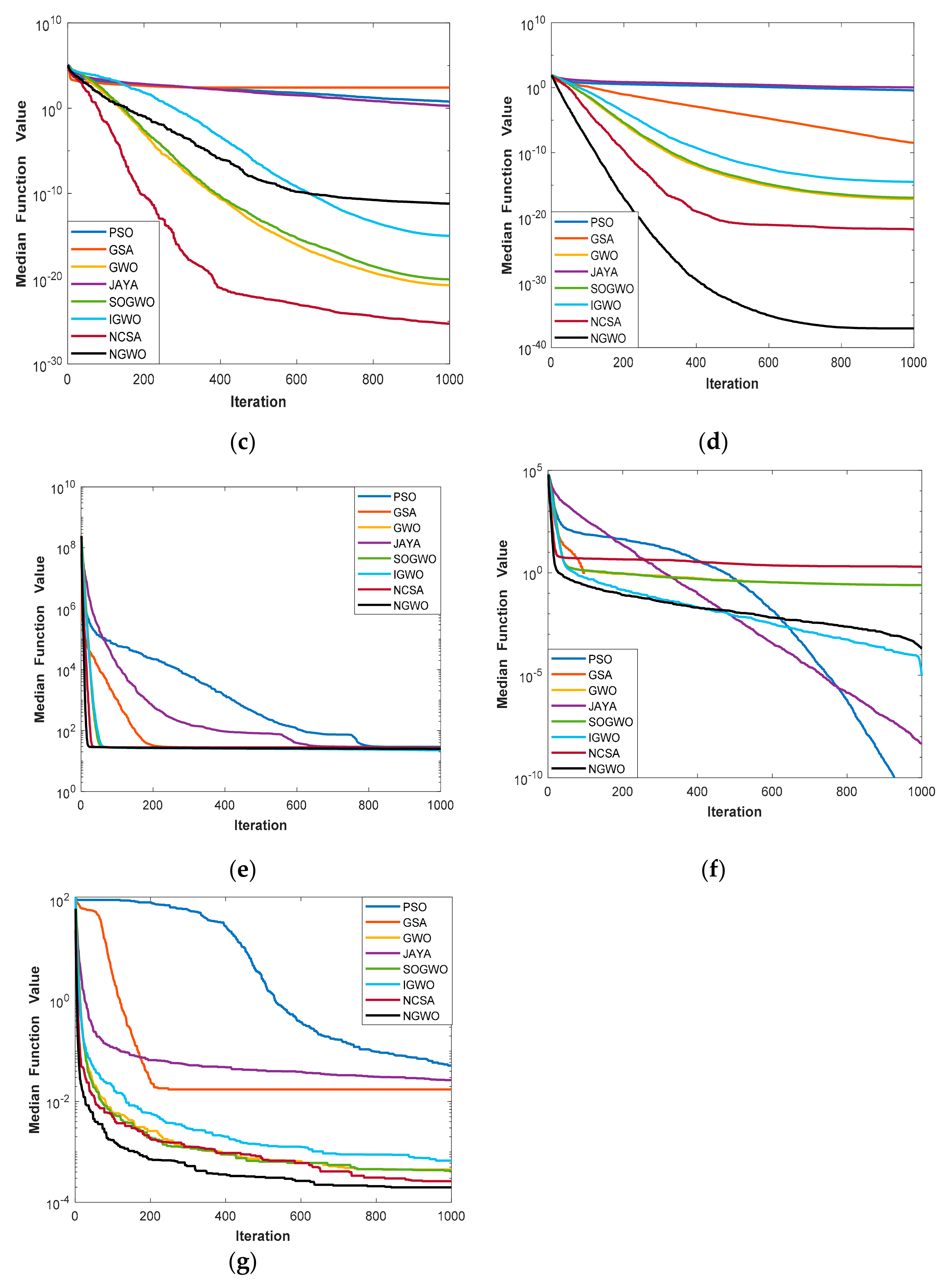
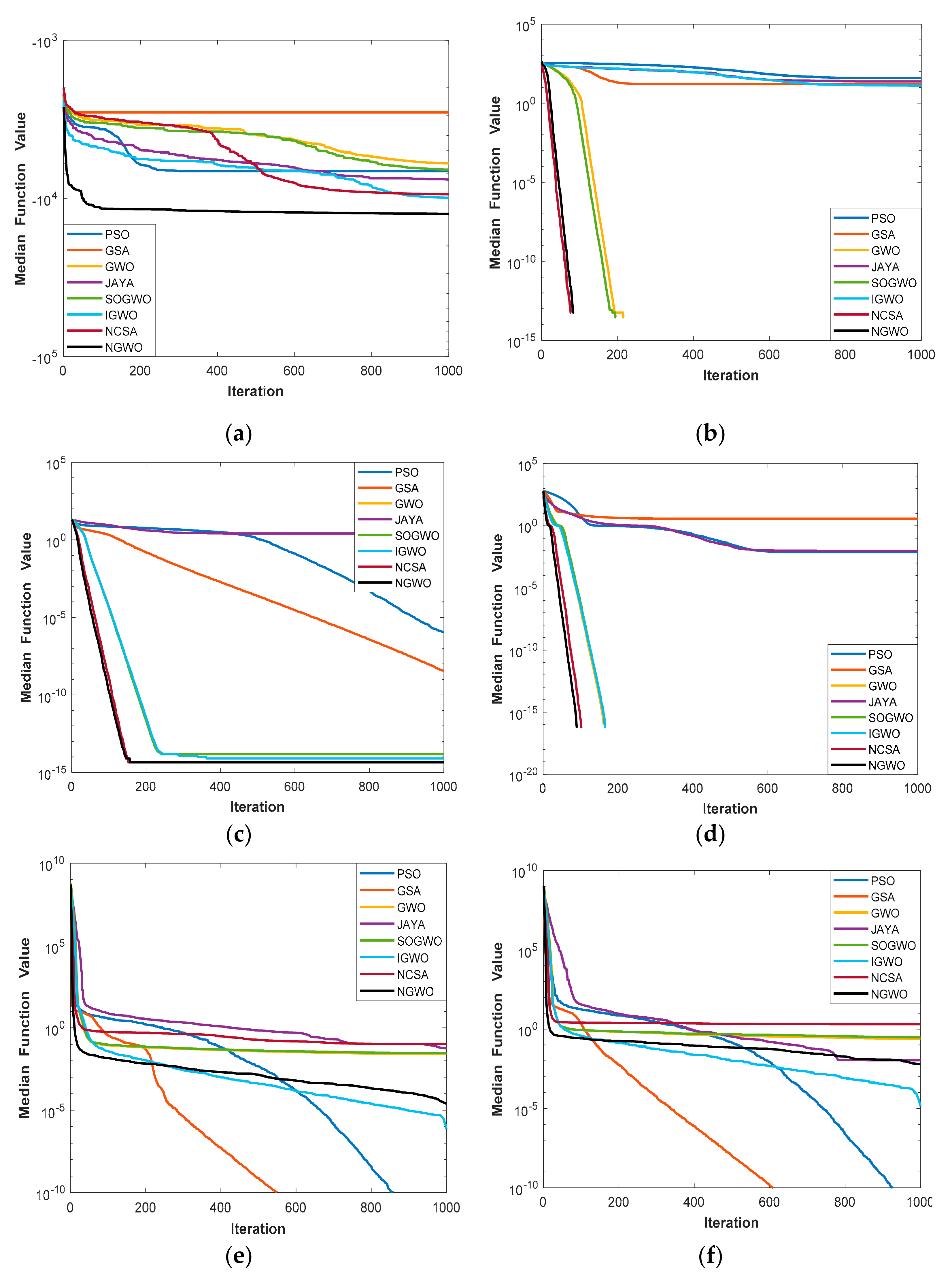
This paragraph illustrates the convergence ability of the NGWO and other compared algorithms. Figure 2 shows the convergence characteristics of the unimodal benchmarks, while Figure 3 depicts the convergence behavior of the six multi-modal benchmarks. In Figure 2 and Figure 3, the horizontal axis signifies the iteration number, and vertical axis shows the median function values from 30 runs. In all Figures, the NGWO maintains a consistent downward slope through the iteration periods, which indicates that the wolves are sharing information to improve the cost function values (fitness) through the iteration period. For most of the convergence curves of Figure 2 and Figure 3, the NGWO shows superior convergence ability that also indicates a proper balance between exploitation and exploration. Furthermore, the NGWO algorithm only took 100 iterations to achieve the exact global optima zero for multi-modal functions F₉ and F₁₁, demonstrating NGWO’s rapid convergence speed.

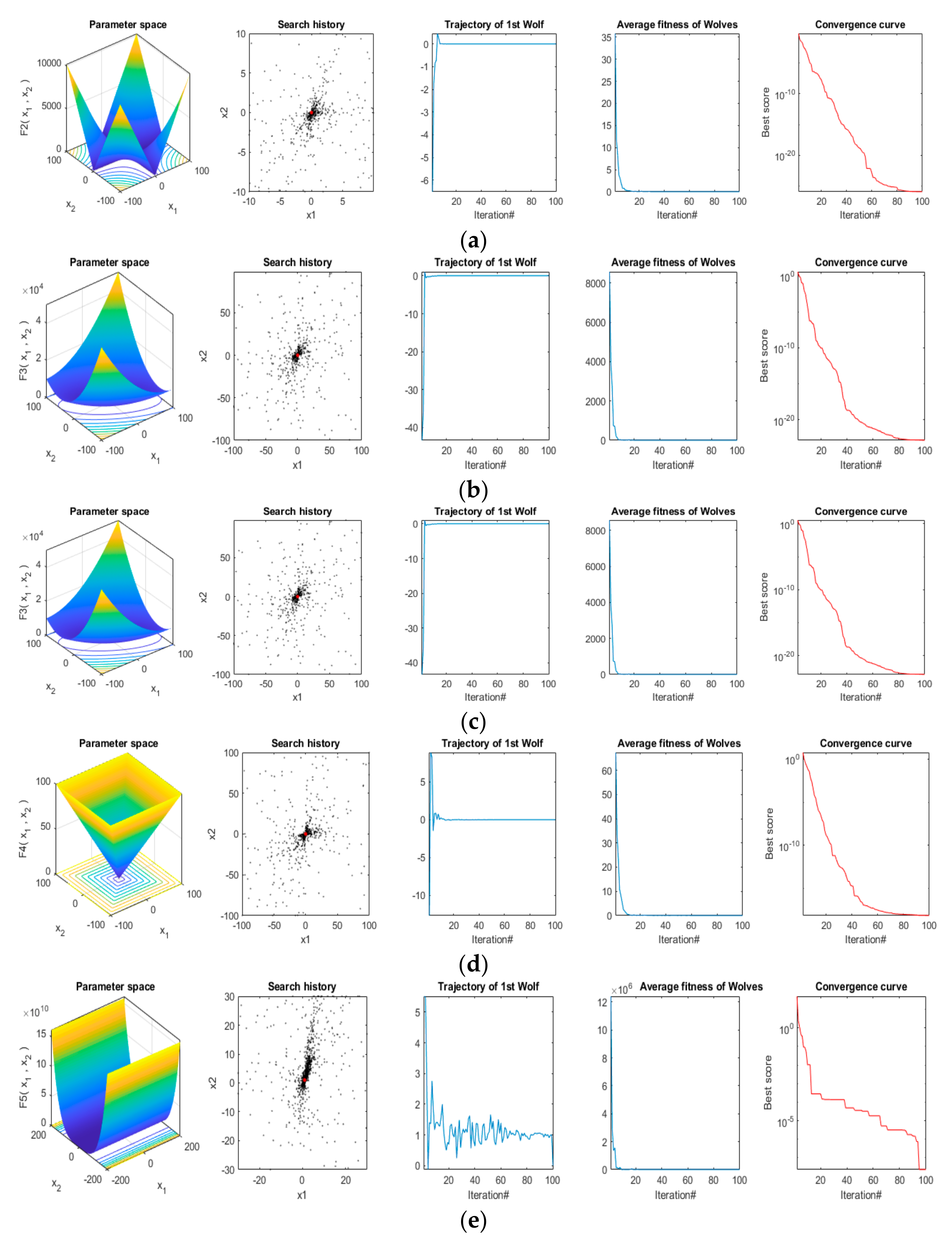
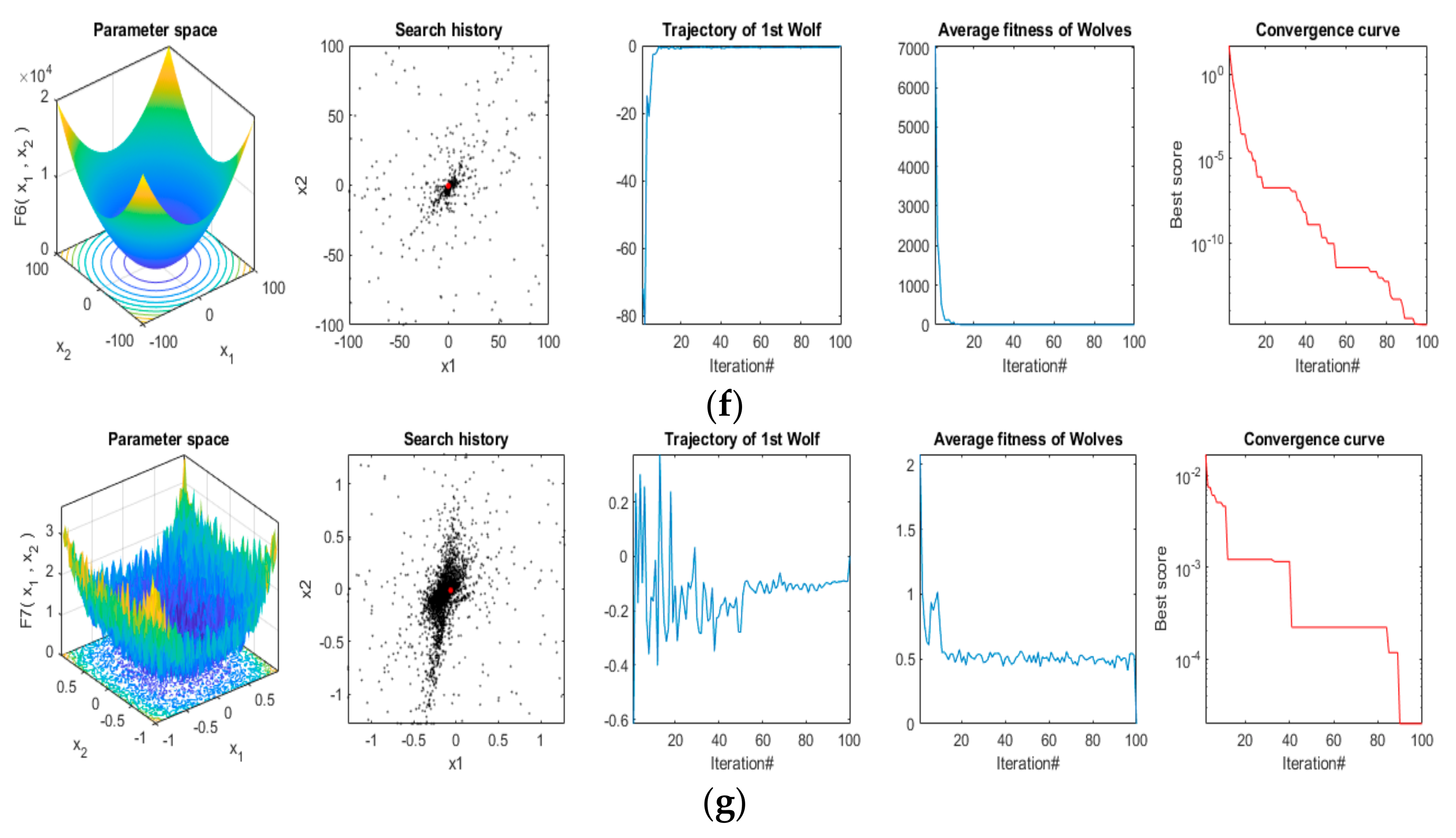
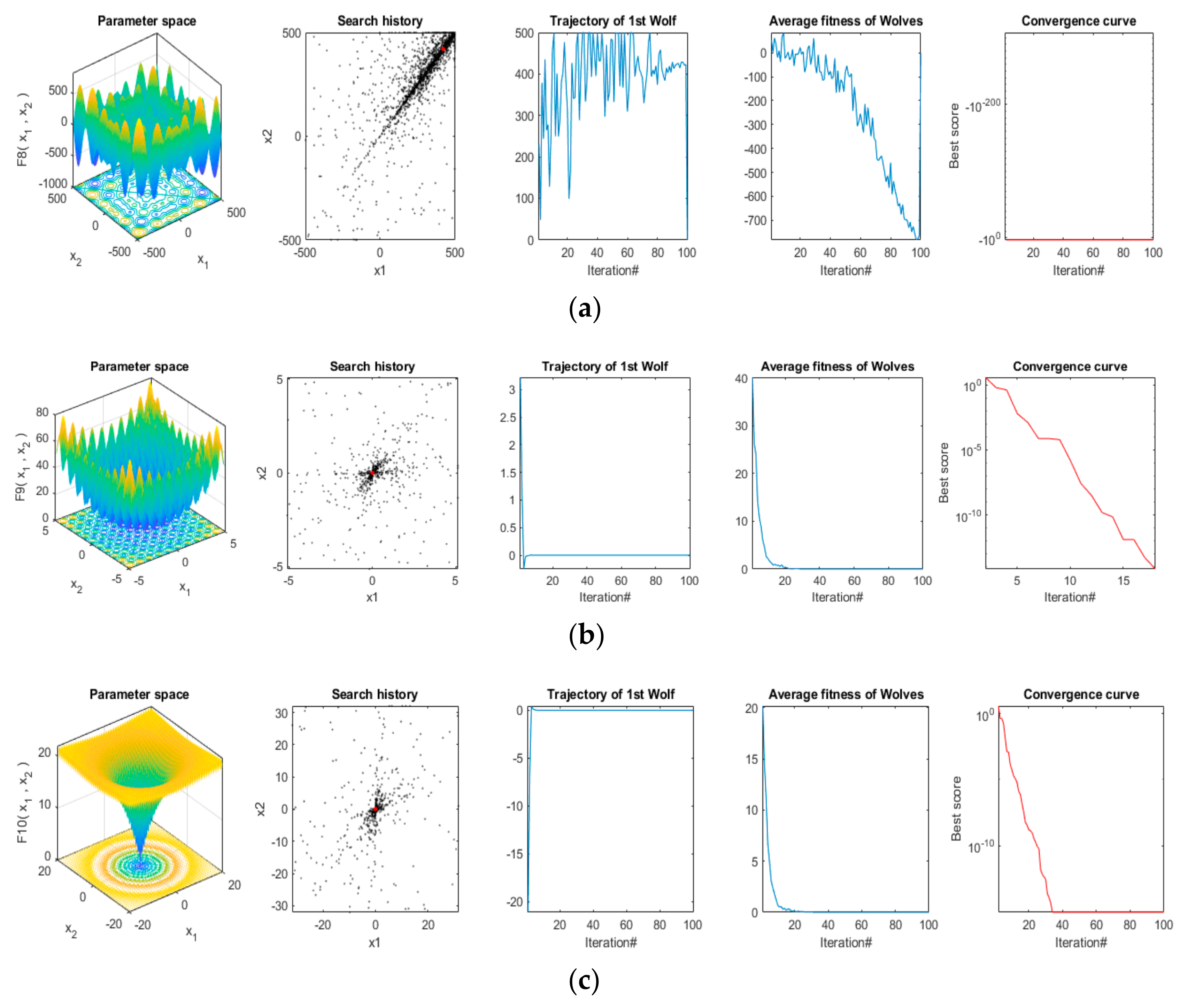
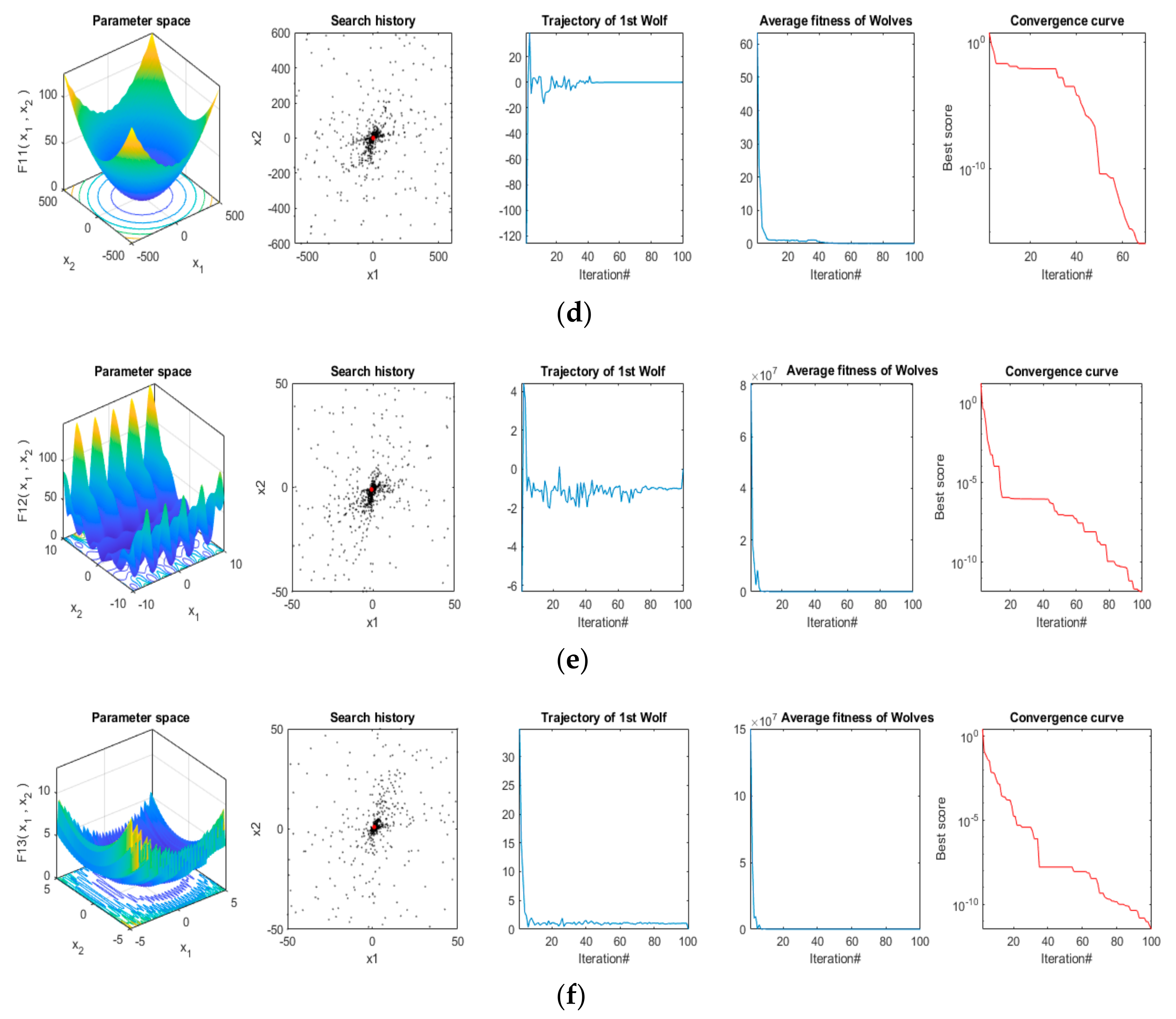
The parameter space, quest history, trajectory of the first wolf, convergence curves, and wolves average fitness are plotted in Figure 4 and Figure 5 to illustrate the convergence behavior in detail. This section has considered the number of wolves and iteration as 50 and 100, respectively. It has been known from the literature [52] that abrupt position changes during the initial iteration steps are more preferable for improving the exploration ability of an algorithm. These changes need to be decreased to strengthen the exploitation ability in the later part of the iteration. The trajectory and search history of the 1st wolf are demonstrated in Figure 4 and Figure 5. It is explicit from the first wolf’s search history (second column of Figure 4 and Figure 5) that the wolves extensively searched through the search space and exploited the best area. The trajectory of 1st wolf (3rd column in Figure 4 and Figure 5) also indicates the same phenomenon, where it emphasized more on exploration in the initial steps, and it decreased through the iteration period. By contrast, the exploitation ability is strengthened during the last periods of iteration. All of these indicate that the NGWO has good convergence ability, and it achieves a proper balance between local exploitation and global exploration.

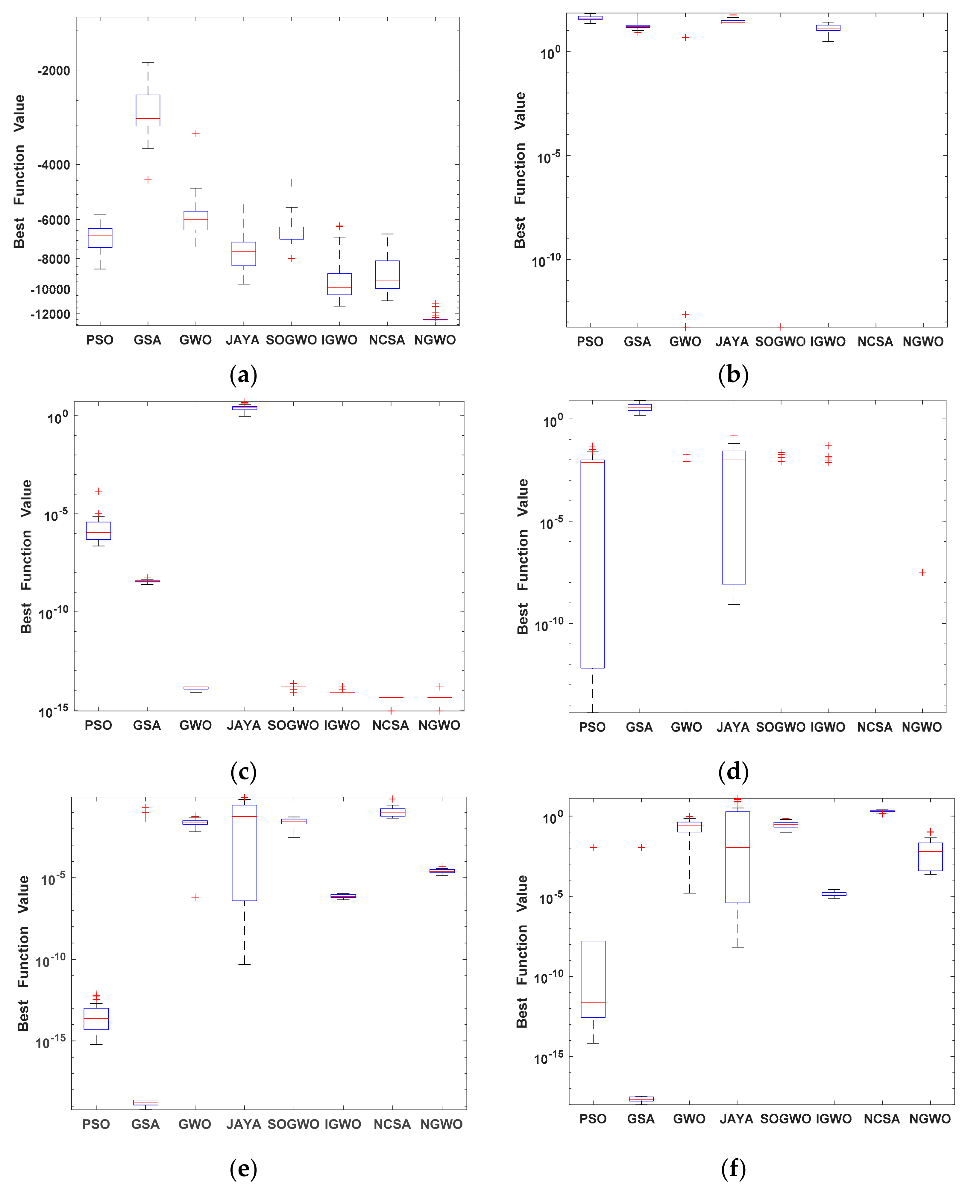
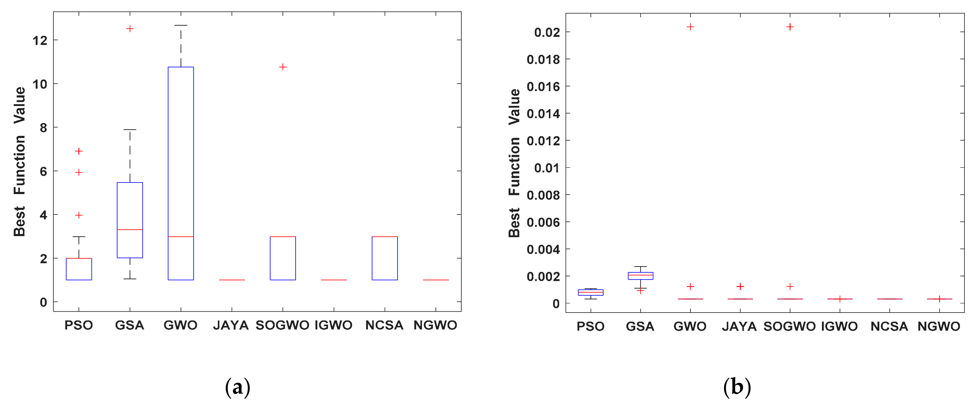
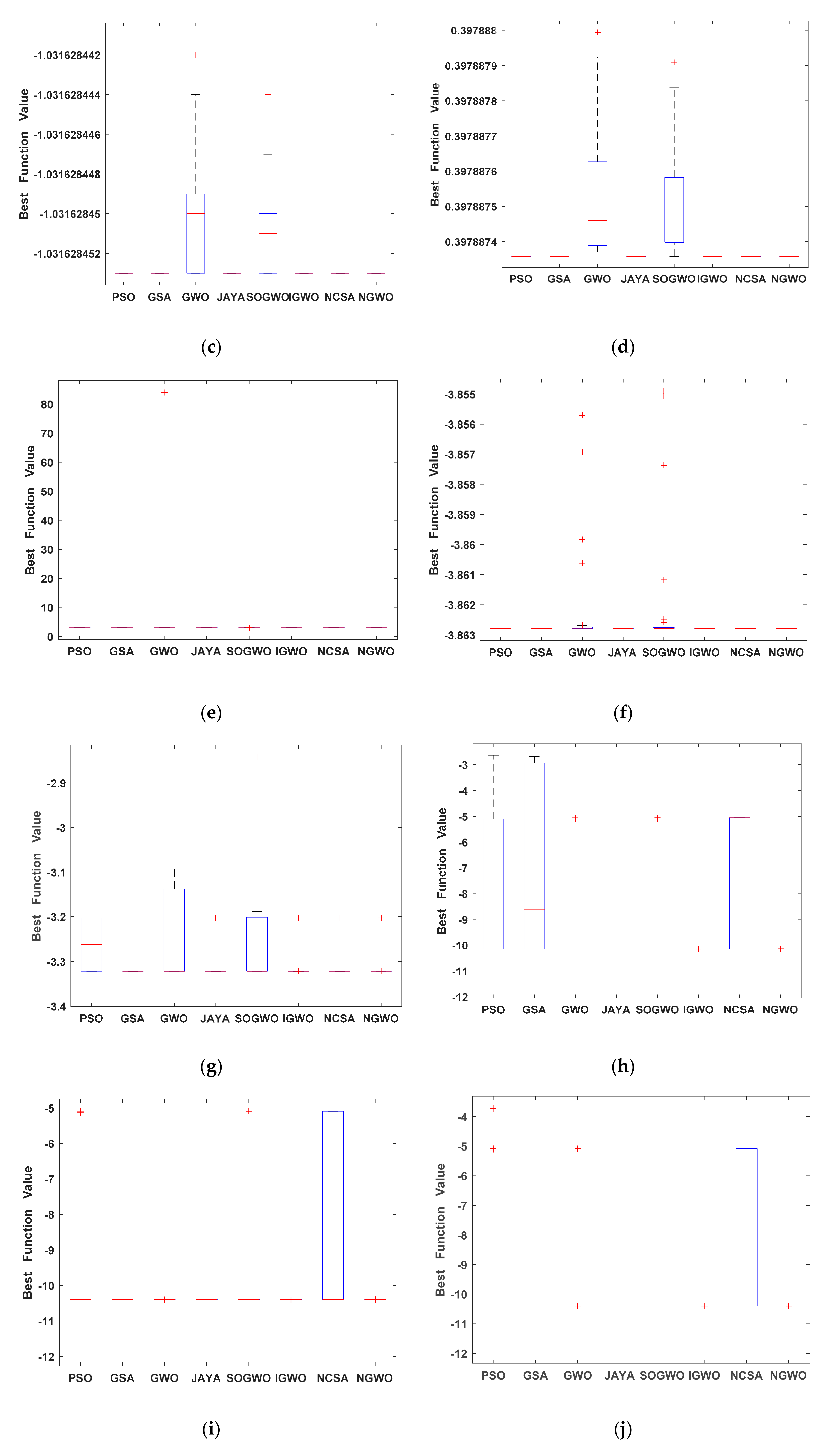
Figure 6 and Figure 7 show the box plots for each algorithm for multi-modal functions. The first six multi-modal functions are 30-dimensional problems (F₇–F₁₃), while the next ten are fixed dimensional multi-modal problems, and the dimension numbers are reported in Table 1. In MATLAB, we run each algorithm 30 times for each test function, saving the best values from each run and plotting them as box plots. These box plots illustrate the distribution of benchmark function results in a better way and indicates the dispersion and symmetry of data sets. The box plots represent the first, second (median), third and lower quartiles, upper bounds and outliers, respectively. The bigger size of the rectangular box indicates that the data sets are scattered more, and the results obtained by the algorithm are not stable. It also indicates the comparatively worst performance. The red crossbar indicates the median of data sets, and the plus sign (+) in red indicates outliers. Among the plots of Figure 6, the box plot location of the NGWO is lower than the other seven algorithms for four functions (F₈–F₁₁, Figure 6a–d), and the box size is also lowest for these functions. In Figure 6b,d the NGWO algorithm reached the exact zero for all data sets, that is why there is no box for NGWO in these two figures. In the case of Figure 7a–j, the NGWO shows the minimum distribution of the data sets and its box plots lies below that of other algorithms. These things indicate the superiority of the proposed NGWO algorithm and less variation in results, and stability of the algorithm.

3.2.4. Ranking of the Algorithms

To analyze the NGWO algorithm’s performance more thoroughly, we conducted non-parametric Friedman tests to rank each algorithm. This multiple comparison test works based on the recurrent measurement of the Anova, and it can determine the differences among the compared algorithms. The best values of each algorithm for 30 runs were stored in a matrix, and the Friedman test was applied to this matrix to obtain the mean ranks of each algorithm for 30 runs. The Friedman test also provides the corresponding p-values for each test function. It is explicit from the Friedman test results in Table 5 that the proposed NGWO attained the best rank for 16 functions among a total of 23 benchmark functions. Additionally, the JAYA, GSA, and PSO obtained the best ranking for 3, 2, and 1 functions, respectively.Very low p–Values indicate that the Friedman test results are statistically significant.

3.3. Engineering Application of NGWO

The proposed algorithm has been tested for three real-life engineering case studies and collected from the literature [18,43]. All three problems have inequality constraints, and we use the hard penalty approach to handle the constraints. We have considered 100 wolves over 100 iterations to solve these three problems.

3.3.1. Welded Beam Design

The objective of this case study is to minimize a welded beam’s fabrication cost. It consists of four decision variables such as bar thickness (b), bar height (t), attached part length (l), and weld thickness (h), and seven inequality constraints (sheer and bending stress, side constraints, end deflection, buckling load). The problem is mathematically formulated as [43]:

$$\mathrm{f}\left(\mathrm{y}\right)=1.10471{\mathrm{y}}_1^2{\mathrm{y}}_2+0.04811{\mathrm{y}}_3{\mathrm{y}}_4\left(14+{\mathrm{y}}_2\right)$$

(34)

$$\mathsf{\tau }\left(\mathrm{y}\right)=\sqrt{{\mathsf{\tau }}_1^2+{\mathsf{\tau }}_1{\mathsf{\tau }}_2\frac{{\mathrm{y}}_2}{2\mathrm{R}}+{\mathsf{\tau }}_2^2}$$

(35)

$${\mathsf{\tau }}_1=\frac{\mathrm{P}}{\sqrt{2}{\mathrm{y}}_1{\mathrm{y}}_2}$$

(36)

$$\mathsf{\tau }2=\frac{\mathrm{MR}}{\mathrm{J}}$$

(37)

$$\mathrm{M}=\mathrm{P}\left(\mathrm{L}+\frac{{\mathrm{y}}_2}{2}\right)$$

(38)

$$\mathrm{R}=\sqrt{0.25*\left({\mathrm{y}}_2^2+{\left({\mathrm{y}}_1+{\mathrm{y}}_3\right)}^2\right)}$$

(39)

$$\mathrm{J}=2/\left\{\sqrt{2}{\mathrm{y}}_1{\mathrm{y}}_2\left[\frac{{\mathrm{y}}_2^2}{12}+\frac{({\mathrm{y}}_1+{\mathrm{y}}_3)^2}{4}\right]\right\}$$

(40)

$$\mathsf{\sigma }\left(\mathrm{y}\right)=\frac{6\mathrm{PL}}{{\mathrm{x}}_4{\mathrm{y}}_3^2}$$

(41)

$$\mathsf{\delta }\left(\mathrm{y}\right)=\frac{4{\mathrm{PL}}^3}{{\mathrm{Ey}}_4{\mathrm{y}}_3^3}$$

(42)

$${\mathrm{P}}_{\mathrm{c}}\left(\mathrm{y}\right)=\frac{4.013{\mathrm{E}\mathrm{y}}_3{\mathrm{y}}_4^3}{6{\mathrm{L}}^2}(1-0.25{\mathrm{y}}_3\sqrt{\left(\frac{\mathrm{E}}{\mathrm{G}}\right)/\mathrm{L})}$$

(43)

Here, $$\begin{gathered} \mathrm{P}=6000\mathrm{l}\mathrm{b}, \mathrm{L}=14 \mathrm{i}\mathrm{n}\mathrm{c}\mathrm{h}, {\mathsf{\delta }}_{\mathrm{m}\mathrm{a}\mathrm{x}}=0.25 \mathrm{i}\mathrm{n}\mathrm{c}\mathrm{h}, \mathrm{E}=30\times {10}^6 \mathrm{p}\mathrm{s}\mathrm{i}, \mathrm{G}=12\times {10}^6\mathrm{p}\mathrm{s}\mathrm{i} , \\ {\mathsf{\tau }}_{\mathrm{m}\mathrm{a}\mathrm{x}}=13600 \mathrm{p}\mathrm{s}\mathrm{i}, {\mathsf{\sigma }}_{\mathrm{m}\mathrm{a}\mathrm{x}}=30000 \mathrm{p}\mathrm{s}\mathrm{i}. \end{gathered}$$ The inequality constraints are:

$${\mathrm{c}}_1\left(\mathrm{y}\right)=\mathsf{\tau }\left(\mathrm{y}\right)-{\mathsf{\tau }}_{\max }\le 0$$

(44)

$${\mathrm{c}}_2\left(\mathrm{y}\right)=\mathsf{\sigma }\left(\mathrm{y}\right)-{\mathsf{\sigma }}_{\max }\le 0$$

(45)

$${\mathrm{c}}_3\left(\mathrm{y}\right)={\mathrm{y}}_1-{\mathrm{y}}_4\le 0$$

(46)

$${\mathrm{c}}_4\left(\mathrm{y}\right)=1.10471{\mathrm{y}}_1^2+0.04811{\mathrm{y}}_3{\mathrm{y}}_4\left(14+{\mathrm{y}}_2\right)-5\le 0$$

(47)

$${\mathrm{c}}_5\left(\mathrm{y}\right)=\mathsf{\delta }\left(\mathrm{y}\right)-{\mathsf{\delta }}_{\max }\le 0$$

(48)

$${\mathrm{c}}_6\left(\mathrm{y}\right)=\mathrm{p}-{\mathrm{p}}_{\mathrm{c}}\left(\mathrm{y}\right)\le 0$$

(49)

$${\mathrm{c}}_7\left(\mathrm{y}\right)=0.125-{\mathrm{y}}_1\le 0$$

(50)

The decision variable bounds are:

$$0.1\le {\mathrm{y}}_1\le 2; 0.1\le {\mathrm{y}}_2\le 10 ; 0.1\le {\mathrm{y}}_3\le 10;0.1\le {\mathrm{y}}_4\le 2$$

3.3.2. Tension–Compression Coil Spring Design

The weight of the tension–compression coil is reduced in this case study. It consists of three decision variables ((number of coils (n), wire diameter (d), mean coil diameter (D)), and 4 inequality constraints. The following is a numerical representation of the problem:

Minimize $\mathrm{f}\left(\mathrm{y}\right)=\left({\mathrm{y}}_3+2\right) {\mathrm{y}}_1{\mathrm{y}}_2^2$

The inequality constraints are:

$${\mathrm{c}}_1\left(\mathrm{y}\right)=1-\frac{{\mathrm{y}}_1^3{\mathrm{y}}_3}{71785{\mathrm{y}}_2^4}\le 0$$

(51)

$${\mathrm{c}}_2\left(\mathrm{y}\right)=\frac{4{\mathrm{y}}_1^2-{\mathrm{y}}_1{\mathrm{y}}_2}{12566\left({\mathrm{y}}_1{\mathrm{y}}_2^3-{\mathrm{y}}_2^4\right)}+\frac{1}{5108{\mathrm{y}}_2^2}-1\le 0$$

(52)

$${\mathrm{c}}_3\left(\mathrm{y}\right)=1-\frac{140.45{\mathrm{y}}_2}{{\mathrm{y}}_1^2{\mathrm{y}}_3}\le 0$$

(53)

$${\mathrm{c}}_4\left(\mathrm{y}\right)=\frac{{\mathrm{y}}_1+{\mathrm{y}}_2}{1.5}-1\le 0$$

(54)

Here, $0.25\le {\mathrm{y}}_1\le 1.30;0.05\le {\mathrm{y}}_2\le 2;2\le {\mathrm{y}}_3\le 15;$

3.3.3. Three Bars Truss Design

Ray and Saini [53] first proposed this case study to minimize the bar’s weight. It has 2 variables and 3 constraints, and it can be mathematically presented as:

Minimize $\mathrm{f}\left(\mathrm{y}\right)=\left(2\sqrt{2} {\mathrm{y}}_1+{\mathrm{y}}_2\right)\times \mathrm{l}$

Subject to

$$\frac{\sqrt{2}{\mathrm{y}}_1+{\mathrm{y}}_2}{\sqrt{2}{\mathrm{y}}_1^2+2{\mathrm{y}}_1{\mathrm{y}}_2}\left(\mathrm{P}-\mathsf{\sigma }\right)\le 0$$

(55)

$$\frac{{\mathrm{y}}_2}{\sqrt{2}{\mathrm{y}}_1^2+2{\mathrm{y}}_1{\mathrm{y}}_2}\left(\mathrm{P}-\mathsf{\sigma }\right)\le 0$$

(56)

$$\frac{1}{2{\mathrm{y}}_1{\mathrm{y}}_2+\sqrt{2}{\mathrm{y}}_1^2}\left(\mathrm{P}-\mathsf{\sigma }\right)\le 0$$

(57)

The variables ranges are: $0\le {\mathrm{y}}_1\le 1 ; 0\le {\mathrm{y}}_2\le 1$ and l = 100 cm, P = 2 KN/cm², and $\mathsf{\sigma }$ = 2 KN/cm²

3.4. Results of the Engineering Application

3.4.1. Optimization Result of Welded Beam Design

It is explicit from the reported results shown in

Table 6. Comparative study of Welded Beam design problem.

Algorithms	y1	y2	y3	y4	f (Best)	f (Mean)	f (Worst)	SD	NFEs
NGWO	0.34094	3.5810	9.0321	0.2063	2.036	2.046	2.0632	1.02 × 102	20,100
GA [54]	0.2489	6.173	8.1789	0.2533	2.4331	N/A	N/A	N/A	N/A
SC [55]	0.2444	6.238	8.2886	0.2446	2.3854	3.2551	6.3997	9.60 × 10−1	33,095
FSA [56]	0.2443	6.2158	8.2939	0.2443	2.3811	2.4042	2.489	N/A	56,243
AATM [57]	0.2441	6.2209	8.2982	0.2444	2.3823	2.387	2.3916	2.20 × 10−3	30,000
HEAA [58]	0.2444	6.2175	8.2915	0.2444	2.381	2.381	2.381	1.30 × 10−5	30,000
EEGWO [41]	0.2444	6.217	8.2928	0.2444	2.3813	2.3817	2.3824	4.18 × 10−4	50,000

that the NGWO outperforms all the previous algorithms for this case study. The proposed algorithm achieved optimal values for four indexes among the five compared indexes (best, mean, worst, standard deviation, and NFEs). In contrast, the HEAA algorithm achieved the best result for the standard deviation index.

3.4.2. Result of Tension–Compression Coil Spring Design

For tension–compression coil spring design, we compared our findings with 10 other previous studies from the literature in

Table 7. Comparative study of tension–compression coil spring design.

Algorithms	y1	y2	y3	f (Best)	f (Mean)	f (Worst)	SD	NFEs
NGWO	10.32826	0.35486	0.05026	0.011053	0.011755	0.012454	5.21 × 10−4	20,100
GA [59]	10.89052	0.36396	0.05198	0.01268	0.01274	0.01297	5.90 × 10−5	80,000
FSA [56]	11.21390	0.35800	0.05174	0.01266	0.01266	0.01266	2.20 × 10−8	49,531
CPSO [60]	11.24454	0.35764	0.05172	0.01267	0.01273	0.01292	5.20 × 10−5	200,000
HPSO [60]	11.26503	0.35712	0.05170	0.01266	0.01270	0.01271	1.58 × 10−5	81,000
GSA [13]	14.22867	0.05	0.31731	0.01287	0.01343	0.01421	1.34 × 10−2	30,000
GWO [18]	12.04249	0.34454	0.05117	0.01267	0.01269	0.01272	2.10 × 10−5	30,000
AFA [61]	11.31956	0.35619	0.05166	0.01266	0.01266	0.01280	1.27 × 10−2	50,000
TEO [62]	11.16839	0.35879	0.05177	0.01266	0.01268	0.01271	4.41 × 10−2	300,000
MGWO [63]	11.80809	0.34819	0.05133	0.01266	0.01267	0.01270	1.10 × 10−5	30,000
EEGWO [41]	11.3113	0.35634	0.05167	0.01266	0.01268	0.01272	2.22 × 10−5	50,000

. The NGWO algorithm achieved the optimal values for four indexes, while the FSA algorithm attained the optimal value for SD index.

3.4.3. Three Bars Truss Design Result

Table 8. Results of three bars truss design problem.

Algorithms	y1	y2	f (Best)	f (Mean)	f (Worst)	SD	NFEs
NGWO	0.789186	0.406806	263.8959	263.8964	263.8971	5.58 × 10−4	20,100
PSO [6]	0.781224	0.432548	264.2183	265.9553	267.459	1.38 × 100	30,000
SC [55]	0.788621	0.408401	263.8958	263.9033	263.9697	1.30 × 10−2	17,610
DEDS [64]	0.788651	0.408316	263.8958	263.8958	263.8958	9.70 × 10−7	15,000
GSA [13]	0.777662	0.448853	264.8299	271.0348	279.7925	4.12 × 100	30,000
HEAA [58]	0.78868	0.408234	263.8958	263.8959	263.8961	4.90 × 10−5	15,000
AATM [57]	0.788682	0.408229	263.8958	263.8966	263.9004	1.10 × 10−3	17,000
WCA [65]	0.788651	0.408316	263.8958	263.8959	263.8962	8.71 × 10−5	5250
MBA [66]	0.788565	0.40856	263.8959	263.898	263.916	3.93 × 10−3	13,280
GWO [18]	0.788409	0.409003	263.8959	263.8966	263.898	4.37 × 10−4	30,000
MVO [67]	0.788993	0.407351	263.8959	263.8961	263.8971	2.49 × 10−4	30,000
SCA [68]	0.789068	0.407162	263.8984	263.9356	263.9951	2.88 × 10−2	30,000
MGWO [63]	0.788561	0.408572	263.8959	263.8963	263.8976	4.29 × 10−4	30,000
EEGWO [41]	0.78841	0.40899	263.896	263.8963	263.8966	2.19 × 10−4	50,000

summarizes the results of three bars truss design problem. The WCA and DEDS algorithms achieved three and two best indexes, respectively. The NGWO algorithm’s results are very similar to the previous best results obtained by various optimization algorithms.

4. Conclusions

The GWO algorithm was influenced by the leadership structure and group hunting system of wolves. The GWO algorithm undergoes the lack of population diversity and is vulnerable to premature convergence in multi-modal problems. Hence, a new variant of GWO called niching GWO (NGWO) with a modified position update equation is proposed in this research to improve the performance of the GWO algorithm for solving multi-modal problems. The niching techniques are well known for handling multiple optimal solutions in the case of multi-modal optimization problems. A fitness Euclidean distance ratio-based niching GWO called FER-GWO is used to strengthen the searchability of the algorithm. By using the FER technique, the wolves are guided towards the nearby wolves’ best position, having better cost function values.

The proposed NGWO algorithm has been thoroughly tested on 23 traditional benchmark functions and three real-world engineering cases. It achieves very promising results and outperforms most other compared algorithms for the considered benchmarks and engineering case studies. This superiority is accomplished by incorporating the niching technique to the basic GWO algorithm and modifying the position update equation, whereas the local search increases the fine searchability. The reported results indicate that the algorithm achieved well-balanced global exploration and local exploitation, which further increases the algorithm’s accuracy. This research focuses on single-objective optimization problems only; however, future work will extend the NGWO algorithm to multi-objective optimization problems.

References

- Xu, X.; Tang, Y.; Li, J.; Hua, C.; Guan, X. Dynamic multi-swarm particle swarm optimizer with cooperative learning strategy. Appl. Soft Comput. 2015, 29, 169–183. [Google Scholar] [CrossRef]
- Qu, B.; Liang, J.; Suganthan, P. Niching particle swarm optimization with local search for multi-modal optimization. Inf. Sci. 2012, 197, 131–143. [Google Scholar] [CrossRef]
- Al Amin, M.; Abdul-Rani, A.M.; Ahmed, R.; Rao, T.V.V.L.N. Multiple-objective optimization of hydroxyapatite-added EDM technique for processing of 316L-steel. Mater. Manuf. Process. 2021, 36, 1–12. [Google Scholar] [CrossRef]
- Holland, J.H. Adaptation in Natural and Artificial Systems: An Introductory Analysis with Applications to Biology, Control, and Artificial Intelligence; The MIT Press: Cambridge, MA, USA, 1975. [Google Scholar]
- Kirkpatrick, S.; Gelatt, C.D.; Vecchi, M.P. Optimization by simulated annealing. Science 1983, 220, 671–680. [Google Scholar] [CrossRef]
- Eberhart, R.; Kennedy, J. A new optimizer using particle swarm theory. In Proceedings of the Sixth International Symposium on Micro Machine and Human Science, MHS’95, Nagoya, Japan, 4–6 October 1995; pp. 39–43. [Google Scholar] [CrossRef]
- Storn, R.; Price, K. Differential evolution—A simple and efficient adaptive scheme for global optimization over continuous spaces. J. Glob. Optim. 1995, 23, 1–15. [Google Scholar]
- Dorigo, M.; Gambardella, L. Ant colony system: A cooperative learning approach to the traveling salesman problem. IEEE Trans. Evol. Comput. 1997, 1, 53–66. [Google Scholar] [CrossRef] [Green Version]
- Lu, X.; Zhou, Y. A novel global convergence algorithm: Bee collecting pollen algorithm. In Advanced Intelligent Computing Theories and Applications. With Aspects of Artificial Intelligence. ICIC 2008. Lecture Notes in Computer Science; Huang, D.S., Wunsch, D.C., Levine, D.S., Jo, K.H., Eds.; Springer: Berlin/Heidelberg, Germany, 2008; Volume 5227. [Google Scholar] [CrossRef]
- Formato, R.A. Central force optimization: A new metaheuristic with applications in applied electromagnetics. Prog. Electromagn. Res. 2007, 77, 425–491. [Google Scholar] [CrossRef] [Green Version]
- Hatamlou, A. Black hole: A new heuristic optimization approach for data clustering. Inf. Sci. 2013, 222, 175–184. [Google Scholar] [CrossRef]
- Tabari, A.; Ahmad, A. A new optimization method: Electro-Search algorithm. Comput. Chem. Eng. 2017, 103, 1–11. [Google Scholar] [CrossRef]
- Rashedi, E.; Nezamabadi-Pour, H.; Saryazdi, S. GSA: A Gravitational Search Algorithm. Inf. Sci. 2009, 179, 2232–2248. [Google Scholar] [CrossRef]
- Rao, R.; Savsani, V.; Vakharia, D. Teaching-learning-based optimization: A novel method for constrained mechanical design optimization problems. Comput. Aided Des. 2011, 43, 303–315. [Google Scholar] [CrossRef]
- Alatas, B. ACROA: Artificial Chemical Reaction Optimization Algorithm for global optimization. Expert Syst. Appl. 2011, 38, 13170–13180. [Google Scholar] [CrossRef]
- Yang, X.S. Firefly algorithm, stochastic test functions and design optimization. Int. J. Bio Inspired Comput. 2010, 2, 78. [Google Scholar] [CrossRef]
- Erol, O.K.; Eksin, I. A new optimization method: Big Bang-Big Crunch. Adv. Eng. Softw. 2006, 37, 106–111. [Google Scholar] [CrossRef]
- Mirjalili, S.; Mirjalili, S.M.; Lewis, A. Grey Wolf Optimizer. Adv. Eng. Softw. 2014, 69, 46–61. [Google Scholar] [CrossRef] [Green Version]
- Mirjalili, S. Dragonfly algorithm: A new meta-heuristic optimization technique for solving single-objective, discrete, and multi-objective problems. Neural Comput. Appl. 2016, 27, 1053–1073. [Google Scholar] [CrossRef]
- Heidari, A.A.; Mirjalili, S.; Faris, H.; Aljarah, I.; Mafarja, M.; Chen, H. Harris hawks optimization: Algorithm and applications. Futur. Gener. Comput. Syst. 2019, 97, 849–872. [Google Scholar] [CrossRef]
- Rao, R.V. Jaya: A simple and new optimization algorithm for solving constrained and unconstrained optimization problems. Int. J. Ind. Eng. Comput. 2016, 7, 19–34. [Google Scholar] [CrossRef]
- Tu, Q.; Chen, X.; Liu, X. Hierarchy strengthened Grey Wolf Optimizer for numerical optimization and feature selection. IEEE Access 2019, 7, 78012–78028. [Google Scholar] [CrossRef]
- Al-Tashi, Q.; Rais, H.M.; Abdulkadir, S.J.; Mirjalili, S. Feature selection based on Grey Wolf Optimizer for oil & gas reservoir classification. In Proceedings of the 2020 International Conference on Computational Intelligence (ICCI), Seri Iskandar, Perak, Malaysia, 8–9 October 2020; pp. 211–216. [Google Scholar] [CrossRef]
- Emary, E.; Zawbaa, H.M.; Grosan, C.; Hassenian, A.E. Feature subset selection approach by gray-wolf optimization. In Advances in Intelligent Systems and Computing; Springer: Cham, Switzerland, 2015; Volume 334. [Google Scholar] [CrossRef]
- Song, J.; Wang, J.; Lu, H. A novel combined model based on advanced optimization algorithm for short-term wind speed forecasting. Appl. Energy 2018, 215, 643–658. [Google Scholar] [CrossRef]
- El-Fergany, A.A.; Hasanien, H.M. Single and multi-objective optimal power flow using Grey Wolf Optimizer and differential evolution algorithms. Electr. Power Compon. Syst. 2015, 43, 1548–1559. [Google Scholar] [CrossRef]
- Sulaiman, M.H.; Mustaffa, Z.; Mohamed, M.R.; Aliman, O. Using the gray wolf optimizer for solving optimal reactive power dispatch problem. Appl. Soft Comput. J. 2015, 32, 286–292. [Google Scholar] [CrossRef] [Green Version]
- Katarya, R.; Verma, O.P. Recommender system with Grey Wolf Optimizer and FCM. Neural Comput. Appl. 2018, 30, 1679–1687. [Google Scholar] [CrossRef]
- Kamboj, V.K. A novel hybrid PSO–GWO approach for unit commitment problem. Neural Comput. Appl. 2016, 27, 1643–1655. [Google Scholar] [CrossRef]
- Panwar, L.K.; Reedy, S.; Verma, A.; Panigrahi, B.K.; Kumar, R. Binary Grey Wolf Optimizer for large scale unit commitment problem. Swarm Evol. Comput. 2018, 38, 251–266. [Google Scholar] [CrossRef]
- Biswas, K.; Vasant, P.M.; Vintaned, J.A.G.; Watada, J. Cellular automata-based multi-objective hybrid Grey Wolf Optimization and particle swarm optimization algorithm for wellbore trajectory optimization. J. Nat. Gas Sci. Eng. 2021, 85, 103695. [Google Scholar] [CrossRef]
- Korayem, L.; Khorsid, M.; Kassem, S.S. Using Grey Wolf algorithm to solve the capacitated vehicle routing problem. Conf. Ser. Mater. Sci. Eng. 2015, 2015, 83. [Google Scholar] [CrossRef] [Green Version]
- Lu, C.; Xiao, S.; Li, X.; Gao, L. An effective multi-objective discrete grey Wolf optimizer for a real-world scheduling problem in welding production. Adv. Eng. Softw. 2016, 99, 161–176. [Google Scholar] [CrossRef] [Green Version]
- Komaki, G.; Kayvanfar, V. Grey Wolf Optimizer algorithm for the two-stage assembly flow shop scheduling problem with release time. J. Comput. Sci. 2015, 8, 109–120. [Google Scholar] [CrossRef]
- Asadzadeh, L. A local search genetic algorithm for the job shop scheduling problem with intelligent agents. Comput. Ind. Eng. 2015, 85, 376–383. [Google Scholar] [CrossRef]
- Jayabarathi, T.; Raghunathan, T.; Adarsh, B.; Suganthan, P.N. Economic dispatch using hybrid grey wolf optimizer. Energy 2016, 111, 630–641. [Google Scholar] [CrossRef]
- Pradhan, M.; Roy, P.K.; Pal, T. Grey Wolf optimization applied to economic load dispatch problems. Int. J. Electr. Power Energy Syst. 2016, 83, 325–334. [Google Scholar] [CrossRef]
- Guha, D.; Roy, P.K.; Banerjee, S. Load frequency control of large scale power system using quasi-oppositional Grey Wolf Optimization algorithm. Eng. Sci. Technol. Int. J. 2016, 19, 1693–1713. [Google Scholar] [CrossRef] [Green Version]
- Singh, N.; Singh, S. A novel hybrid GWO-SCA approach for optimization problems. Eng. Sci. Technol. Int. J. 2017, 20, 1586–1601. [Google Scholar] [CrossRef]
- Jiang, T.; Zhang, C. Application of Grey Wolf Optimization for solving combinatorial problems: Job Shop and Flexible Job Shop scheduling cases. IEEE Access 2018, 6, 26231–26240. [Google Scholar] [CrossRef]
- Long, W.; Jiao, J.; Liang, X.; Tang, M. An exploration-enhanced Grey Wolf Optimizer to solve high-dimensional numerical optimization. Eng. Appl. Artif. Intell. 2018, 68, 63–80. [Google Scholar] [CrossRef]
- Dhargupta, S.; Ghosh, M.; Mirjalili, S.; Sarkar, R. Selective opposition based Grey Wolf Optimization. Expert Syst. Appl. 2020, 151, 113389. [Google Scholar] [CrossRef]
- Nadimi-Shahraki, M.H.; Taghian, S.; Mirjalili, S. An improved Grey Wolf Optimizer for solving engineering problems. Expert Syst. Appl. 2021, 166, 113917. [Google Scholar] [CrossRef]
- Yin, X.; Germay, N. A Fast genetic algorithm with sharing scheme using cluster analysis methods in multimodal function optimization. In Artificial Neural Nets and Genetic Algorithms; Springer: Cham, Switzerland, 1993. [Google Scholar]
- Mahfound, S.W. Crowding and preselection revisited. In Parallel Problem Solving from Nature; Elsevier: Amsterdam, The Netherlands, 1992. [Google Scholar]
- Petrowski, A. Clearing procedure as a niching method for genetic algorithms. In Proceedings of the IEEE International Conference on Evolutionary Computation, Nayoya, Japan, 20–22 May 1996. [Google Scholar] [CrossRef]
- Li, X. Niching without niching parameters: Particle swarm optimization using a ring topology. IEEE Trans. Evol. Comput. 2010, 14, 150–169. [Google Scholar] [CrossRef]
- Li, X. A multimodal particle swarm optimizer based on fitness Euclidean-distance ratio. In Proceedings of the 9th Annual Conference on Genetic and Evolutionary Computation—GECCO ’07, London, UK, 7–11 July 2007; pp. 78–85. [Google Scholar] [CrossRef] [Green Version]
- Li, X. Adaptively choosing neighbourhood bests using species in a particle swarm optimizer for multimodal function optimization. In Proceedings of the Genetic and Evolutionary Computation Conference 2004, Seattle, WA, USA, 26–30 June 2004; pp. 105–116. [Google Scholar] [CrossRef]
- Islam, J.; Rahaman, A.; Vasant, P.; Negash, B.; Hoqe, A.; Alhitmi, H.K.; Watada, J. A modified niching crow search approach to well placement optimization. Energies 2021, 14, 857. [Google Scholar] [CrossRef]
- Peram, T.; Veeramachaneni, K.; Mohan, C.K. Fitness-distance-ratio based particle swarm optimization. In Proceedings of the 2003 IEEE Swarm Intelligence Symposium. SIS’03, Indianapolis, IN, USA, 24–26 April 2003. [Google Scholar] [CrossRef]
- Bergh, F.V.D.; Engelbrecht, A.P. A study of particle swarm optimization particle trajectories. Inf. Sci. 2006, 176, 937–971. [Google Scholar] [CrossRef]
- Ray, T.; Saini, P. Engineering design optimization using a swarm with an intelligent information sharing among individuals. Eng. Optim. 2001, 33, 735–748. [Google Scholar] [CrossRef]
- Deb, K. Optimal design of a welded beam via genetic algorithms. AIAA J. 1991, 29, 2013–2015. [Google Scholar] [CrossRef]
- Ray, T.; Liew, K. Society and civilization: An optimization algorithm based on the simulation of social behavior. IEEE Trans. Evol. Comput. 2003, 7, 386–396. [Google Scholar] [CrossRef]
- Hedar, A.-R.; Fukushima, M. Derivative-free filter simulated annealing method for constrained continuous global optimization. J. Glob. Optim. 2006, 35, 521–549. [Google Scholar] [CrossRef]
- Wang, Y.; Cai, Z.; Zhou, Y. Accelerating adaptive trade-off model using shrinking space technique for constrained evolutionary optimization. Int. J. Numer. Methods Eng. 2009, 77, 1501–1534. [Google Scholar] [CrossRef]
- Wang, Y.; Cai, Z.; Zhou, Y.; Fan, Z. Constrained optimization based on hybrid evolutionary algorithm and adaptive constraint-handling technique. Struct. Multidiscip. Optim. 2008, 37, 395–413. [Google Scholar] [CrossRef]
- Coello, C.A.C.; Montes, E.M. Constraint-handling in genetic algorithms through the use of dominance-based tournament selection. Adv. Eng. Inform. 2002, 16, 193–203. [Google Scholar] [CrossRef]
- He, Q.; Wang, L. An effective co-evolutionary particle swarm optimization for constrained engineering design problems. Eng. Appl. Artif. Intell. 2007, 20, 89–99. [Google Scholar] [CrossRef]
- Baykasoğlu, A.; Ozsoydan, F.B. Adaptive firefly algorithm with chaos for mechanical design optimization problems. Appl. Soft Comput. J. 2015, 36, 152–164. [Google Scholar] [CrossRef]
- Kaveh, A.; Dadras, A. A novel meta-heuristic optimization algorithm: Thermal exchange optimization. Adv. Eng. Softw. 2017, 110, 69–84. [Google Scholar] [CrossRef]
- Kumar, V.; Kumar, D. An astrophysics-inspired Grey Wolf algorithm for numerical optimization and its application to engineering design problems. Adv. Eng. Softw. 2017, 112, 231–254. [Google Scholar] [CrossRef]
- Zhang, M.; Luo, W.; Wang, X. Differential evolution with dynamic stochastic selection for constrained optimization. Inf. Sci. 2008, 178, 3043–3074. [Google Scholar] [CrossRef]
- Eskandar, H.; Sadollah, A.; Bahreininejad, A.; Hamdi, M. Water cycle algorithm—A novel metaheuristic optimization method for solving constrained engineering optimization problems. Comput. Struct. 2012, 110–111, 151–166. [Google Scholar] [CrossRef]
- Sadollah, A.; Bahreininejad, A.; Eskandar, H.; Hamdi, M. Mine blast algorithm: A new population based algorithm for solving constrained engineering optimization problems. Appl. Soft Comput. 2013, 13, 2592–2612. [Google Scholar] [CrossRef]
- Mirjalili, S.; Mirjalili, S.M.; Hatamlou, A. Multi-Verse Optimizer: A nature-inspired algorithm for global optimization. Neural Comput. Appl. 2016, 27, 495–513. [Google Scholar] [CrossRef]
- Mirjalili, S. SCA: A Sine Cosine Algorithm for solving optimization problems. Knowl. Based Syst. 2016, 96, 120–133. [Google Scholar] [CrossRef]
Figure 1.
Steps of the NGWO algorithm.
Figure 2.
Convergence characteristics of the algorithms for unimodal benchmark functions (F1–F7). Here, (a) represents benchmark function F1, (b) represents benchmark function F2, (c) represents benchmark function F3, (d) represents benchmark function F4, (e) represents benchmark function F5, (f) represents benchmark function F6, (g) represents benchmark function F7.
Figure 3.
Convergence characteristics of the algorithms for multi-modal benchmark functions (F8-F13). Here, (a) represents benchmark function F8, (b) represents benchmark function F9, (c) represents benchmark function F10, (d) represents benchmark function F11, (e) represents benchmark function F12, (f) represents benchmark function F13.
Figure 4.
Parameter space, search history, trajectory of 1st wolf, the average fitness of all wolves, and convergence curve of NGWO for unimodal functions (F1–F7). Here, (a) represents benchmark function F1, (b) represents benchmark function F2, (c) represents benchmark function F3, (d) represents benchmark function F4, (e) represents benchmark function F5, (f) represents benchmark function F6, (g) represents benchmark function F7.
Figure 5.
Parameter space, search history, trajectory of 1st wolf, the average fitness of wolves, and convergence curve of NGWO for multi-modal functions (F8–F13). Here, (a) represents benchmark function F8, (b) represents benchmark function F9, (c) represents benchmark function F10, (d) represents benchmark function F11, (e) represents benchmark function F12, (f) represents benchmark function F13.
Figure 6.
Box plot of the multi-modal benchmark functions (F8–F13). Here, (a) represents F8, (b) represents F9, (c) represents F10, (d) represents F11, (e) represents F12, (f) represents F13.
Figure 7.
Box plot of the fixed dimensional multi-modal benchmark functions (F14–F23). Here, (a) represents benchmark function F14, (b) represents benchmark function F15, (c) represents benchmark function F16, (d) represents benchmark function F17, (e) represents benchmark function F18, (f) represents benchmark function F19, (g) represents benchmark function F20, (h) represents benchmark function F21, (i) represents benchmark function F22, (j) represents benchmark function F23.