Study of Image Classification Accuracy with Fourier Ptychography

Abstract

In this research, the accuracy of image classification with Fourier Ptychography Microscopy (FPM) has been systematically investigated. Multiple linear regression shows a strong linear relationship between the results of image classification accuracy and image visual appearance quality based on PSNR and SSIM with multiple training datasets including MINST, Fashion MNIST, Cifar, Caltech 101, and customized training datasets. It is, therefore, feasible to predict the image classification accuracy only based on PSNR and SSIM. It is also found that the image classification accuracy of FPM reconstructed with higher resolution images is significantly different from using the lower resolution images under the lower numerical aperture (NA) condition. The difference is yet less pronounced under the higher NA condition.

1. Introduction

Fourier Ptychography Microscopy (FPM) is a computational microscopy imaging technique potentially able to achieve a wide field of view and high-resolution imaging. It involves the use of a sequence of LEDs (LED array), which illuminates sequentially onto the target. Based on the sequential illumination, iterated sampling methods in the frequency domain are used for recovering higher resolution images [1,2,3]. Different types of Fourier Ptychography techniques have been proposed in the past for improving imaging resolutions [1,2,3,4,5,6,7]. Among them, multiplexed coded illumination techniques, laser-based implementations, aperture scanning Fourier Ptychography, camera scanning Fourier Ptychography, multi-camera approach, single-shot Fourier Ptychography, speckle illumination, X-ray Fourier Ptychography, and diffuser modulation have achieved successes [1]. More recent research has specifically addressed the Fourier Ptychography imaging problems such as the brightfield, phase, darkfield, reflective, multi-slice, and fluorescence imaging [3,4,5].

Driven by the significant interests in deep learning, a few different methods have been developed to solve the ill-posed Fourier Ptychography imaging problems. Notably, a convolutional neural network has been successfully applied for solving the Fourier Ptychography imaging problem [7]. The U-Net type structure-based generative adversarial network (GAN) was used to utilize fewer samples (26 images versus a few hundred images) for obtaining similar quality image reconstruction [8]. More promisingly, the U-Net plus GAN structure is proven able to reconstruct the high-resolution images using only a smaller amount of lower resolution image input data [9]. An interpretable deep learning approach has shown its effectiveness for the imaging of scattering materials [9,10].

Until recently, the majority of Fourier Ptychography imaging studies have been primarily focusing on achieving high-resolution imaging based on the criteria of human visual perception satisfaction, yet a significant question left to answer is to understand the impact of such a technique on the broad spectrum of the downstream image processing related visual tasks such as classification, segmentation, and object detection. The ability to answer these questions is critical for applications such as industrial robotics, medical imaging, and industrial automation [10,11].

It is well known that deep learning is time-consuming, thus imposing significant computational challenges. However, a significant research effort has been made where the recent breakthrough has shown that the training time of Imagenet has been reduced from days to hours, even further to minutes [12]. All these breakthroughs, however, come with a price. They all require expensive GPU devices for training the deep learning neural network. The expenses of the costly hardware can be well reflected through the price of the GPU card, for example, an NVIDIA P-100 GPU card costs about USD 6000 with the current market [12]. Training of all possible combinations of the different quality of FPM reconstructions for obtaining image classification accuracy is feasible but time-consuming and costly. As such, it is desirable to formulate the relationships between the FPM reconstructed image quality and the image classification accuracy in order to avoid training all the different combinations of the data and still able to identify the optimal parameters used for FPM reconstruction to achieve the best performance of the image classification accuracy [13,14,15,16,17,18,19,20].

With this research, we propose to use the Fourier Ptychography technique to reconstruct higher (FPM-based) and lower resolution (without FPM) images for image classification. Following the FPM reconstruction, a deep convolution neural network is constructed for evaluation of the image recognition accuracy for both higher and lower resolution images. A multiple linear regression model is used to regress the relationship between independent variables including peak signal to noise ratio (PSNR), the structural similarity index (SSIM), and the dependent variable image classification accuracy. Based on the regression model, it becomes feasible to infer the image classification accuracy directly based on PSNR and SSIM rather than through the intensive and time-consuming deep learning-based image classification training. In comparison to deep learning image classification training, PSNR and SSIM are easier to calculate with lower computational cost, the proposed method then becomes useful for predicting the image classification accuracy of FPM-related visual tasks. Additionally, our research also provides insights into the general effectiveness of image classification accuracy following FPM reconstruction by comparing the FPM reconstruction with or without FPM reconstruction (also known as higher or lower resolution images). In conclusion, our contribution of using PSNR and SSIM to predict image classification accuracy is not only limited to the FPM technique but also a universal approach to other imaging techniques such as digital holography, optical scanning holography, and transport of intensity imaging [21,22].

2. Methodology

2.1. Fourier Ptychography

For the imaging task, given an object complex field ${\mathrm{O}}_0\left(\mathrm{x},\mathrm{y}\right)$ with spectrum represented by ${\mathrm{O}}_0\left({\mathrm{k}}_{\mathrm{x}},{\mathrm{k}}_{\mathrm{y}}\right)$, where ${\mathrm{k}}_{\mathrm{x}}$ and ${\mathrm{k}}_{\mathrm{y}}$ denote the spatial frequencies along the x and y-direction. The n-th captured low-resolution raw image intensity is ${\mathrm{I}}_{\mathrm{n}}\left(\mathrm{x},\mathrm{y}\right)$ (n = 1, 2, 3…N) with a spectrum of ${\mathrm{G}}_{\mathrm{n}}\left({\mathrm{k}}_{\mathrm{x}},{\mathrm{k}}_{\mathrm{y}}\right)$. The coherent transfer function (CTF) of the microscope objective is given as $\mathrm{C}\left({\mathrm{k}}_{\mathrm{x}},{\mathrm{k}}_{\mathrm{y}}\right)=\mathrm{circ}\left({\mathrm{k}}_{\mathrm{r}}/{\mathrm{k}}_0\mathrm{NA}\right)$, where ${\mathrm{k}}_{\mathrm{r}}=\sqrt{{\mathrm{k}}_{\mathrm{x}}^2+{\mathrm{k}}_{\mathrm{y}}^2}$, ${\mathrm{k}}_{\mathrm{x}}$ and ${\mathrm{k}}_{\mathrm{y}}$ represent the spatial frequencies along the x and y directions. denotes a value 1 within a circle of radius ${\mathrm{r}}_0$ and 0 otherwise, and $\mathrm{r}=\sqrt{{\mathrm{x}}^2+{\mathrm{y}}^2}$. NA is the numerical aperture of the microscope objective and finally ${\mathrm{k}}_0$ is the wavenumber of the light source.

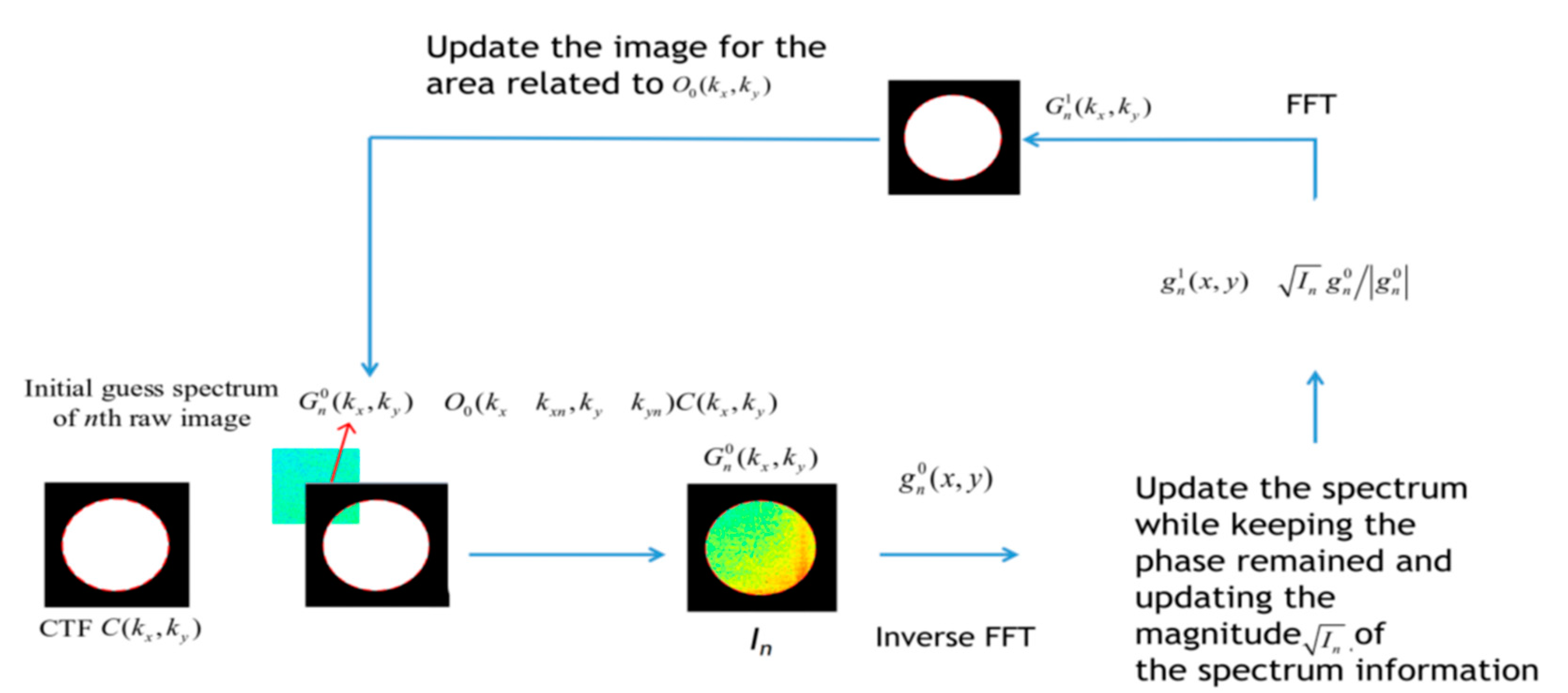
The FPM reconstruction starts from an initial guess of the spectrum distribution of the nth raw image, ${\mathrm{G}}_{\mathrm{n}}^0\left({\mathrm{k}}_{\mathrm{x}},{\mathrm{k}}_{\mathrm{y}}\right)$, according to:

$${\mathrm{g}}_{\mathrm{n}}^0\left(\mathrm{x},\mathrm{y}\right)={\Im }^{-1}\left\{{\mathrm{G}}_{\mathrm{n}}^0\left({\mathrm{k}}_{\mathrm{x}},{\mathrm{k}}_{\mathrm{y}}\right)\right\}={\Im }^{-1}\left\{{\mathrm{O}}_0\left({\mathrm{k}}_{\mathrm{x}}-{\mathrm{k}}_{\mathrm{xn}},{\mathrm{k}}_{\mathrm{y}}-{\mathrm{k}}_{\mathrm{yn}}\right)\mathrm{C}\left({\mathrm{k}}_{\mathrm{x}},{\mathrm{k}}_{\mathrm{y}}\right)\right\}$$

(1)

where $\Im$ and ${\Im }^{-1}$ represent Fourier transform and inverse Fourier transform. k_xn and ${\mathrm{k}}_{\mathrm{yn}}$ indicate the phase-shift caused by the oblique illumination along the x and y directions. To update ${\mathrm{g}}_{\mathrm{n}}^0$, we replace the amplitude of ${\mathrm{g}}_{\mathrm{n}}^0$ with $\sqrt{{\mathrm{I}}_{\mathrm{n}}}$ as:

$${\mathrm{g}}_{\mathrm{n}}^1\left(\mathrm{x},\mathrm{y}\right)=\sqrt{{\mathrm{I}}_{\mathrm{n}}}\frac{{\mathrm{g}}_{\mathrm{n}}^0}{\left|{\mathrm{g}}_{\mathrm{n}}^0\right|}$$

(2)

The superscript indices 0 and 1 in ${\mathrm{g}}_{\mathrm{n}}\left(\mathrm{x},\mathrm{y}\right)$ represent the prior and post updated low-resolution image, respectively. The updated spectrum is ${\mathrm{G}}_{\mathrm{n}}^1\left({\mathrm{k}}_{\mathrm{x}},{\mathrm{k}}_{\mathrm{y}}\right)=\Im \left\{{\mathrm{g}}_{\mathrm{n}}^1\left(\mathrm{x},\mathrm{y}\right)\right\}$, as such the updated spectrum ${\mathrm{O}}_0^1\left({\mathrm{k}}_{\mathrm{x}},{\mathrm{k}}_{\mathrm{y}}\right)$ is:

$${\mathrm{O}}_0^1\left({\mathrm{k}}_{\mathrm{x}}-{\mathrm{k}}_{\mathrm{xn}},{\mathrm{k}}_{\mathrm{y}}-{\mathrm{k}}_{\mathrm{xn}}\right)={\mathrm{O}}_0\left({\mathrm{k}}_{\mathrm{x}}-{\mathrm{k}}_{\mathrm{xn}},{\mathrm{k}}_{\mathrm{y}}-{\mathrm{k}}_{\mathrm{yn}}\right)\left[1-\mathrm{C}\left({\mathrm{k}}_{\mathrm{x}},{\mathrm{k}}_{\mathrm{y}}\right)\right]+{\mathrm{G}}_{\mathrm{n}}^1\left({\mathrm{k}}_{\mathrm{x}},{\mathrm{k}}_{\mathrm{y}}\right)$$

(3)

Repeating Equations (1) to (3) by using ${\mathrm{I}}_{\mathrm{n}}$ from $\mathrm{n}=1$ to $\mathrm{n}=\mathrm{N}$ in one iteration, following convergence, the error function ${\mathrm{E}}_{\mathrm{k}}$ becomes:

$${\mathrm{E}}_{\mathrm{k}}={{\displaystyle \sum }}_{\mathrm{n}=1}^{\mathrm{N}}{{\displaystyle \sum }}_{\mathrm{x},\mathrm{y}}{\left\{\left|{\mathrm{g}}_{\mathrm{k},\mathrm{n}}^1\left(\mathrm{x},\mathrm{y}\right)\right|-\sqrt{{\mathrm{I}}_{\mathrm{n}}\left(\mathrm{x},\mathrm{y}\right)}\right\}}^2,$$

(4)

The second summation indicates the pixel-by-pixel summation for every single image. In ${\mathrm{g}}_{\mathrm{k},\mathrm{n}}^0$, the superscript indices 0 and k represent the complex distribution of the n-th low-resolution image before the k-th iteration is completed. Following the k-th iteration, the high-frequency component-maintained spectrum ${\mathrm{O}}_{\mathrm{k}}\left({\mathrm{k}}_{\mathrm{x}},{\mathrm{k}}_{\mathrm{y}}\right)$ is recovered. The intensity distribution of it is:

$${\mathrm{I}}_{\mathrm{k}}={\left|{\mathrm{O}}_{\mathrm{k}}\left(\mathrm{x},\mathrm{y}\right)\right|}^2={\left|{\Im }^{-1}\left\{{\mathrm{O}}_{\mathrm{k}}\left({\mathrm{k}}_{\mathrm{x}},{\mathrm{k}}_{\mathrm{y}}\right)\right\}\right|}^2$$

(5)

${\mathrm{O}}_{\mathrm{k}}\left({\mathrm{k}}_{\mathrm{x}},{\mathrm{k}}_{\mathrm{y}}\right)$ of Equation (5) indicates the desired spectrum after the k-th iteration, correspondingly, the ${\mathrm{O}}_0\left({\mathrm{k}}_{\mathrm{x}},{\mathrm{k}}_{\mathrm{y}}\right)$ indicates the original spectrum prior to the iteration of the update, the same as to ${\mathrm{I}}_{\mathrm{k}}$ and ${\mathrm{O}}_{\mathrm{k}}\left(\mathrm{x},\mathrm{y}\right)$. Figure 1 shows the sequence of the FPM algorithm.

In simulation, we choose to use a 630 nm red laser. Camera CCD resolution is 2.76 µm. The distance between the LED array and the sample is 90 mm. The gap between LEDs is 4 mm. The Fourier Ptychography image reconstruction process starts from the lower resolution direct images. In our study, we used 225 slower resolution images (15 × 15 LED array). Based on the 225 lower resolution images, we continued to perform spectrum sampling in the frequency domain. Based on Equation (2), the higher resolution image spectrum was updated until the converging condition specified was reached as shown in Equation (3). For the purpose of comparison between the FPM reconstructed image (the higher resolution) and the lower resolution image (the raw lower resolution image, without going through the FPM reconstruction process), the middle LED of the 15 by 15 LED array was chosen to be used. The system numerical aperture (NA) chosen here was varied from 0.05 to 0.5.

2.2. Image Classification

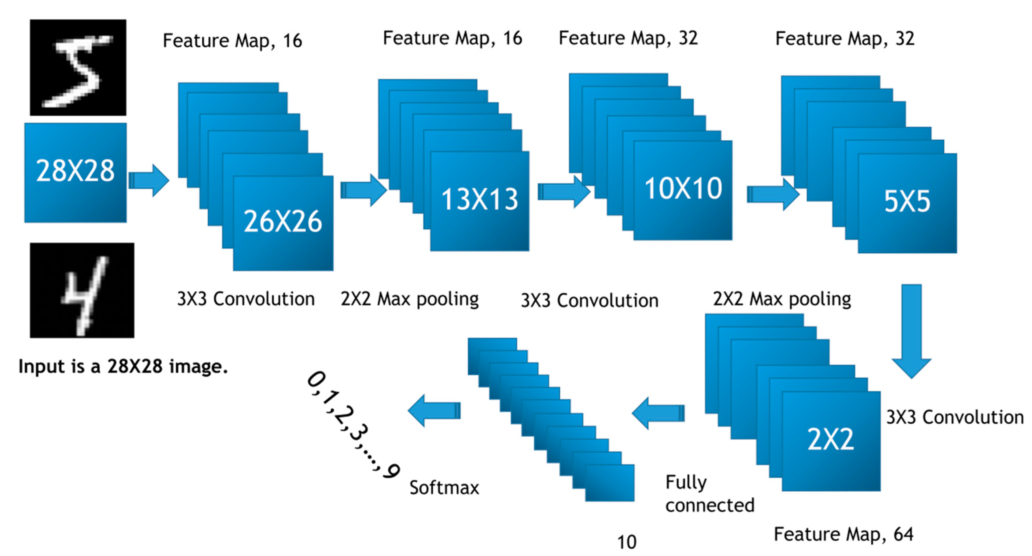
For the evaluation of the accuracy of image classification, a deep convolution neural network was used. We used six different neural networks for systematic image classification. The first deep convolution neural network was designed to train the MNIST dataset. The architecture of the convolution neural network is shown in Figure 2. In this convolution neural network, the following structure was used. Given the input size of 28 by 28 images, a 3 by 3 convolution is performed. Following the 3 by 3 convolution, a feature map of size 26 by 26 was obtained. There was a total of 16 such feature maps obtained. A 2 by 2 max-pooling was consequently performed. It produced a 13 by 13 feature map, where in total 16 such feature maps were obtained. A 3 by 3 convolution was further processed. Therefore, this lead to 32 10 by 10 feature maps. Continuously, a 2 by 2 max-pooling was conducted, yielding 32 feature maps at the size of 5 by 5. It follows that the 3 by 3 convolution operation yielded a 2 by 2 feature map with a total of 64 such feature maps. The fully connected operation was also conducted yielding a fully connected layer at the size of 10. Finally, softmax was performed for image classification.

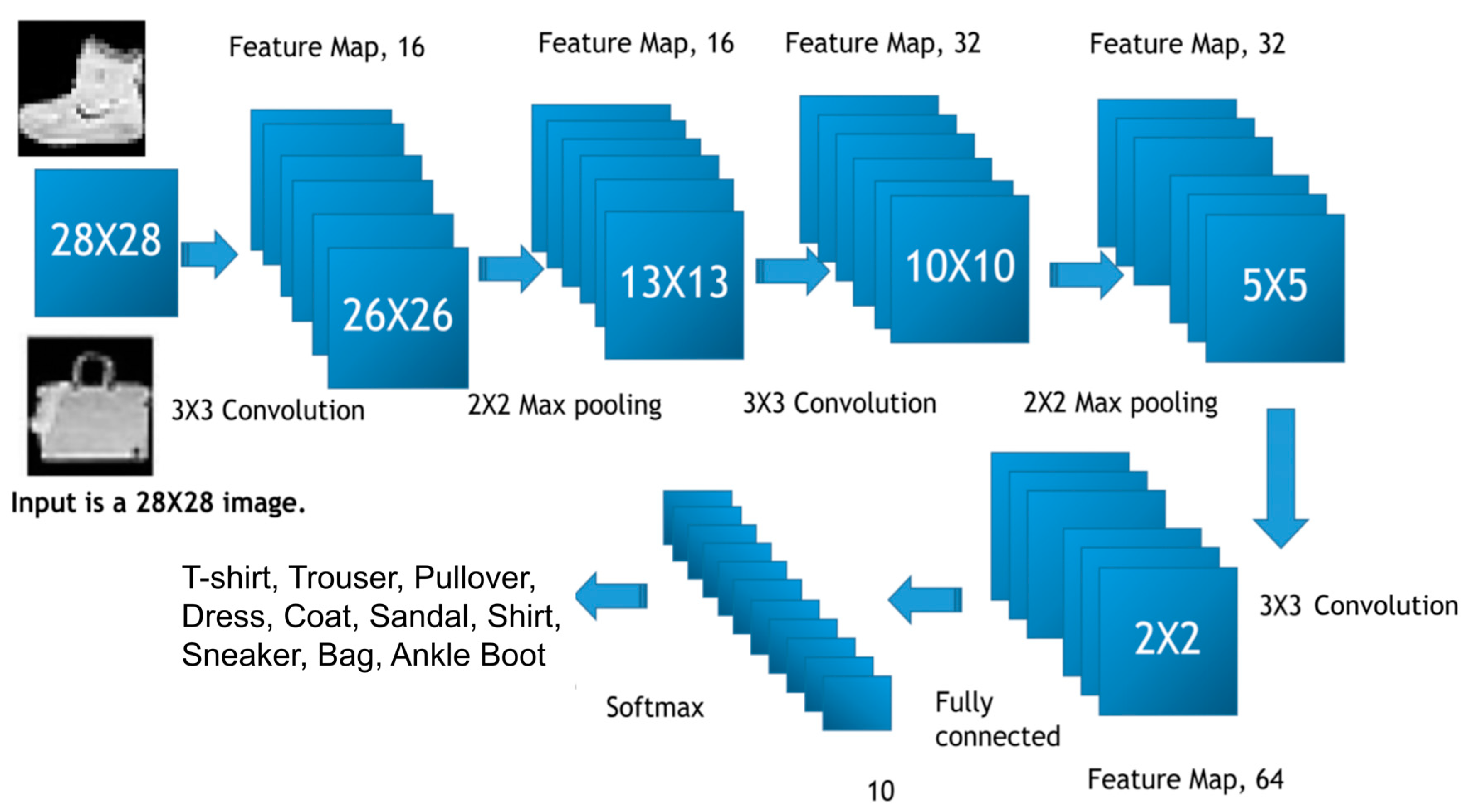
Similarly, the same network architecture was also used for the Fashion-MNIST dataset training as shown in Figure 3. The Fashion-MNIST dataset is built following the principle of MNIST dataset. It has an identical format to the MNIST dataset in terms of image size, but has a more complex geometry including 11 classes of t-shirt, trouser, dress, coat, sandal, shirt, sneaker, bag, and ankle boot [14]. It is known that Fashion-MNIST is a more challenging data benchmark for image classification tasks [15].

It is worthwhile to note that the purpose of our research was not to achieve the highest image classification accuracy, but rather, we wanted to compare the image classification accuracy between an FPM reconstructed image (higher resolution) versus the lower resolution image (raw lower resolution image collected). We also want to discover the relationship between PSNR, SSIM, and image classification accuracy. As such, we only randomly chose part of the entire 60,000 images. Through our experiment, we discovered that the use of a partial set of images is able to achieve reasonable training accuracy while preventing overfitting. Thus, in this research, we chose to use 2560 MNIST images for performing training. By doing this, there are two advantages, first, the use of fewer images enabled us to do more rapid training. For example, training 50,000 FPM-processed images requires over 30 h on a moderate performance laptop. Yet, training of 2560 images requires nearly 20 times less training time. This allows us to do multiple trainings given different NAs within a reasonable time frame, thus were are able to build the regression model between PSNR, SSIM, and classification accuracy. However, the principles of the method proposed in this research were able to be universally applied to an arbitrary number of images for training and evaluation.

Similarly, for Fashion-MNIST, 2560 FPM processed images were used for training. A total of 512 FPM-processed images were used for the evaluation of the classification accuracy. Stochastic gradient descent with momentum was used as the optimizer for both MNIST and Fashion-MNIST training. Compared to batch stochastic gradient descent, minibatch stochastic gradient descent is more capable of reducing the training error, as such, it is also adopted to reduce the training error to the smallest. The training learning rate was chosen as 0.0001. For all the convolution layers, a padding of 1 was used. Eighty epochs were iterated before the training stopped.

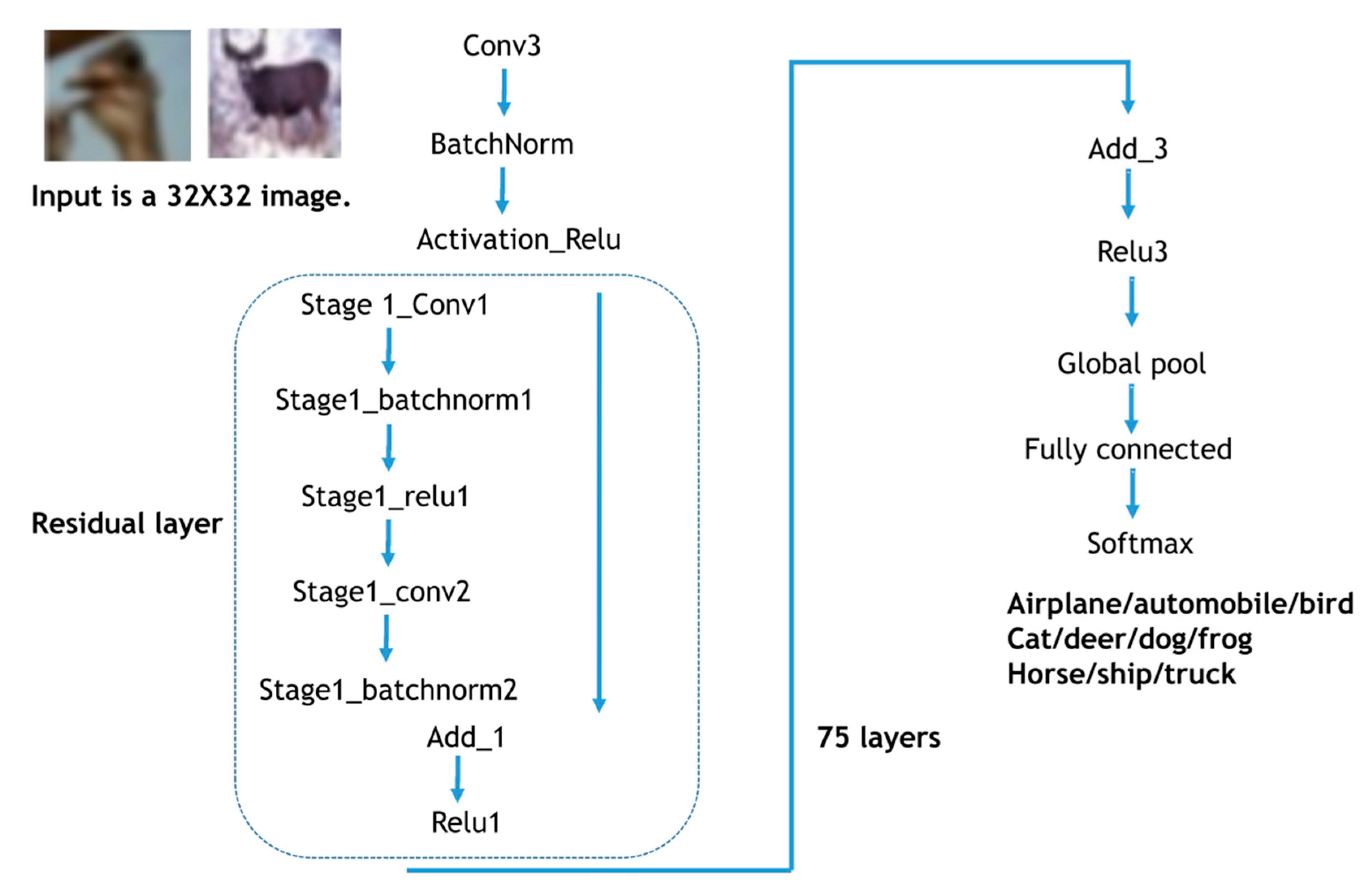
The CIFAR dataset was also used for both training and evaluation. The CIFAR dataset includes 10 classes of airplane, automobile, bird, cat, deer, dog, frog, horse, ship, and truck. Differently, images from the CIFAR dataset have three channels (RGB), whereas both MNIST and Fashion-MNIST only have a single channel. Among them, similar to MNIST and Fashion-MNIST, 2560 FPM-processed images were used for training, and 512 FPM-processed images were used for evaluation of the classification accuracy. The residual type of neural network structure was adopted for training and evaluation purposes. The residual network structure is known to enable deeper layers of a network without the vanishing gradient problem [16]. It suggests that even with deeper layers, the training is still able to converge within a reasonable amount of training time. The residual network is also able to perform well on image feature maps fusion, taking advantage of its unique long-short memory mechanisms, and thus achieving better image classification accuracy [16]. The learning rate was chosen as 0.1. In total, 80 epochs during training were conducted. The residual network structure is shown in Figure 4. In order to reduce the likelihood of over-fitting, image augmentation is conducted including image translation and reflection. Cropping is performed prior to the start of training [17].

The Caltech 101 dataset ass also used for training. Within Caltech 101, there are 101 classes including plane, chair, soccer, brain, and others. Each class has about 60 images. In total, 25 categories were used for training and evaluation. In contrast to MNIST, Fashion-MNIST and the CIFAR image set have limited resolutions of 28 by 28 and 32 by 32. Caltech 101 image resolution is much higher, mostly with a size of 300 by 200. The use of large images can better ensure the FPM image reconstruction accuracy. The FPM reconstruction method involves iteratively sampling the overlap region of the lower resolution images in the frequency domain. As such, a larger input can help to improve the reconstruction accuracy [1]. With the inclusion of larger input images, the input dataset becomes richer. With the richer input dataset, it is also helpful to build a more diversified relationship model between image classification, PSNR, and SSIM. Similar to the training performed against the CIFAR dataset, the deep residual network, resnet50, was used for the image classification task shown in Figure 5. The neural network had 177 layers connected by the residual blocks among the inter layers. Before the training started, color and cropping-based image augmentation was performed to reduce the likelihood of image overfitting [17,18]. Note that the linear activation function (Relu) was used in the residual network. The function was able to train a deeper neural network without the vanishing gradient problem because the activation function had the advantages of both linear and nonlinear transformations of the input. The batch normalization reduced the value variation for each layer, thus increasing the stability of the deep network training and reducing the needed epochs for achieving the ideal classification accuracy.

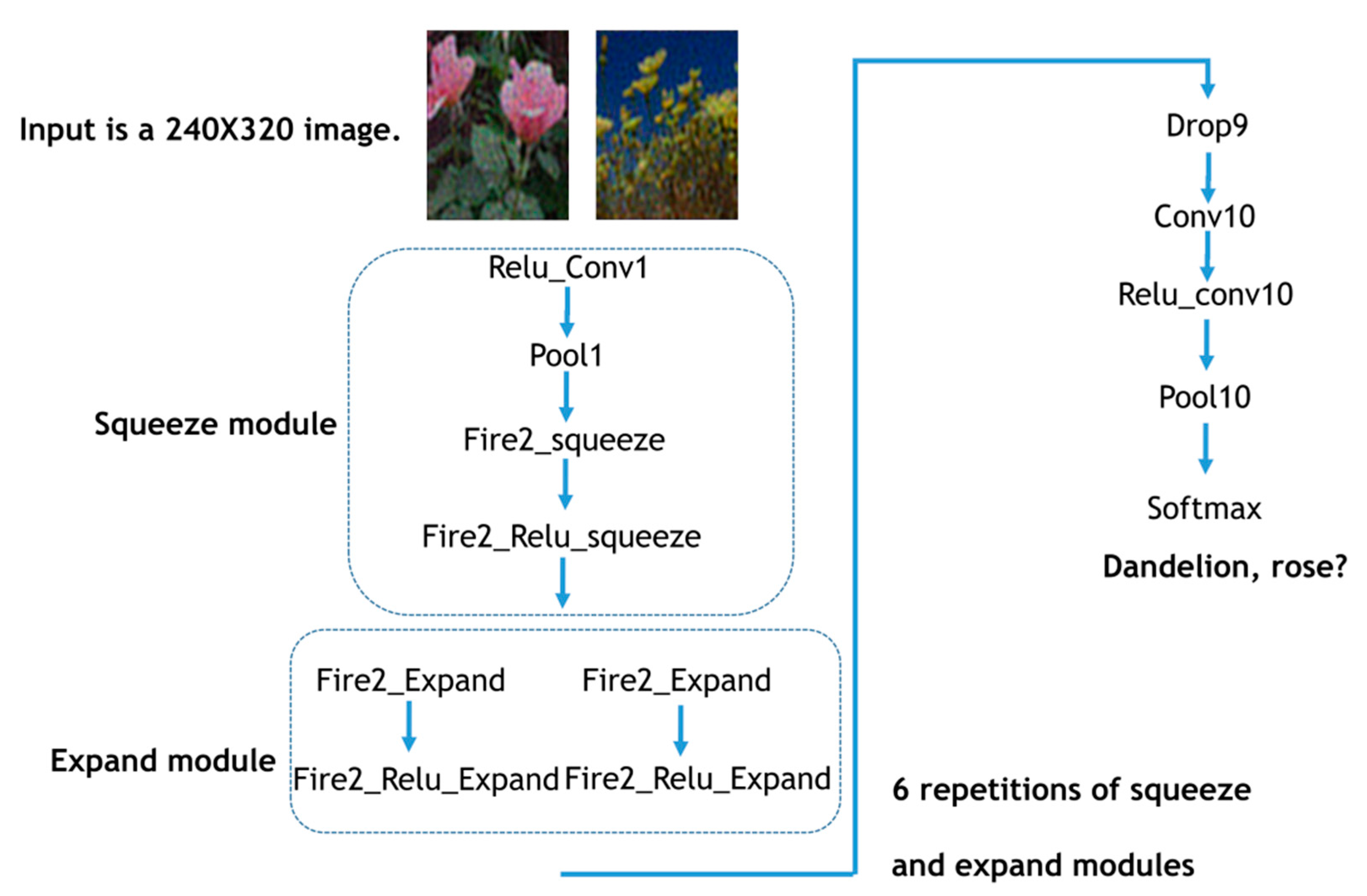
The use of customized data for testing the image classification accuracy with and without FPM reconstruction was also conducted. For this, two customized training data were included, namely the flowers and apple pathology datasets. The flowers dataset included 4242 images with sub-categories of daisy, dandelion, flowers, rose, sunflower, and tulip. The number of images per category were balanced. The balanced apple pathology data had 3200 images. Blackrot, cedar rust, scab, and healthy apples were included. For the flowers dataset, SqueezeNet was used for the classification of different types of flowers shown in Figure 6. The SqueezeNet consists of repeated Squeeze and expansion neural network modules. The Squeeze and fire modules employ a 1 by 1 filter. The direct benefit of using a 1 by 1 convolution filter is that the network requires fewer parameters and more memory efficient. The subsequent downsampling (e.g., pool10) enables the larger activation map, thus is beneficial for maximizing the classification accuracy.

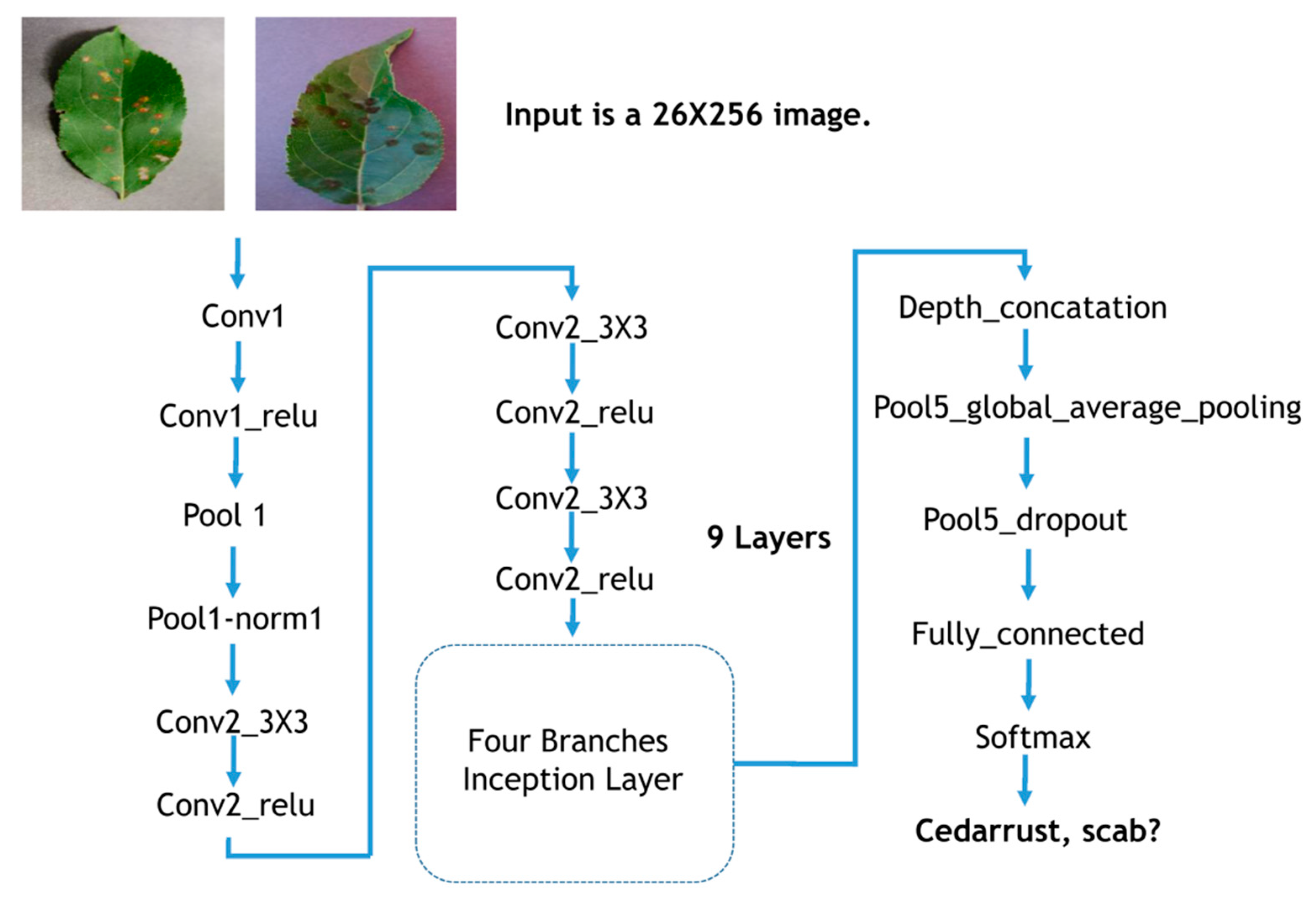
For the apple pathology dataset, a Google inception-based network was used for the classification of the apple diseases shown in Figure 7. Google inception employs the inception layer as the backbone of the network. In total, nine repeated inception modules were used. Within the inception modules, different sizes of filters were used. Among them, 1 by 1, 3 by 3, and 5 by 5 filters were used within the inception module. By doing this, it can save weight parameters of the deep network. Additionally, by dividing the sequential filters into four branches within the inception layer, it further reduced the numbers of parameters, thus enabling a further increase in the computational efficiency.

Through training, a fine-tuned approach is utilized. The beginning three layers of the network are frozen and only the last two layers are trained. The data are augmented through reflection along one side of the image, followed by random translation and scaling along both sides of the image. A minimum batch size of 5 was used per batch throughout the training process. Random shuffling of the data was performed to reduce the likelihood of over-fitting. Twenty percent of the data was used for validation of the training accuracy. For achieving good training accuracy, a small initial learning rate of 0.0003 was used. In total, 6 epochs of training was found to be sufficient for achieving a converged training accuracy.

Following the training of the MNIST, Fashion-MNIST, CIFAR, Caltech 101, flowers, and apple pathology datasets, the image classification accuracy was obtained for the FPM reconstructed image, lower resolution image, as well as the ground truth image. Furthermore, PSNR and SSIM are also calculated for the FPM reconstructed image, lower resolution image, as well as ground truth image. The calculation of PSNR and SSIM values uses the ground truth image as the reference. Multiple linear regression is also performed for the PSNR, SSIM (independent variables), and image classification accuracy (dependent variable). A p-value of 0.05 is used as the significance threshold of the F-Test performed against the goodness of fit of the regression.

3. Results

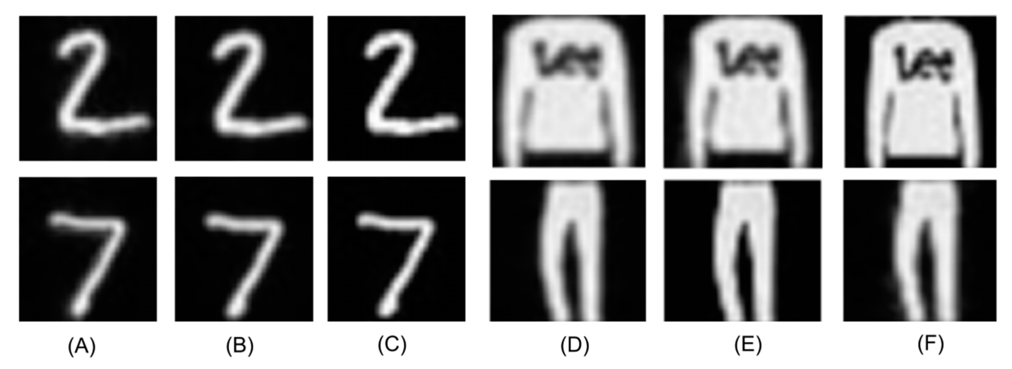
The results of Fourier Ptychography are shown in Figure 8, Figure 9, Figure 10 for different datasets. Figure 8 shows the results using MNIST and Fashion-MNIST.

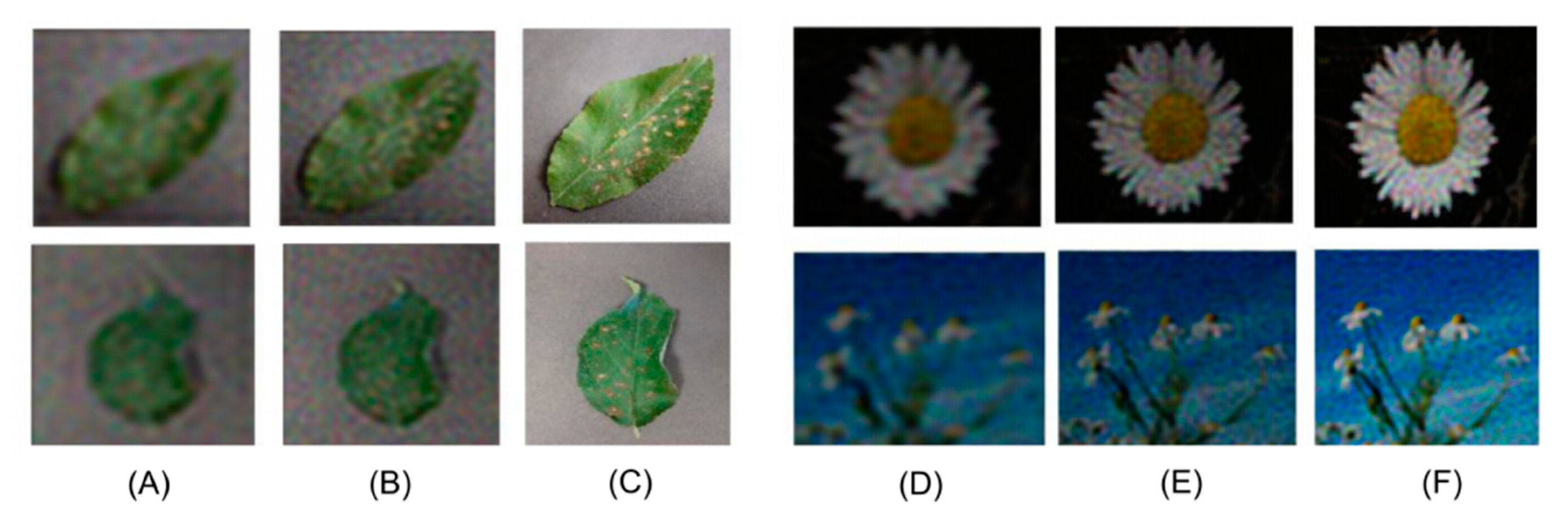
Lower resolution image, FPM reconstructed image, and original image based on CIFAR and CalTech 101 are shown in Figure 9. Similarly, the lower resolution image, FPM reconstructed image, and original image based on the flowers and apple pathology datasets are shown in Figure 10. Consistently, all four datasets show their effectiveness in the generation of higher resolution images using FPM reconstruction.

The results of PSNR and SSIM, and classification accuracy for CIFAR, CalTech101, MNIST, Fashion-MNIST, flowers, and apple pathology datasets are shown in

Table 1. PSNR, SSIM, and classification accuracy for CIFAR and CalTech101.

Dataset	Numerical Aperture	Reconstruction Method	PSNR	SSIM	Classification Accuracy
CIFAR	Ground Truth		Inf	1	76.61%
	0.5	FPM	14.64	0.79	61.72%
		Lower Resolution	14.39	0.76	58.79%
	0.2	FPM	14.46	0.78	59.38%
		Lower Resolution	13.81	0.61	52.74%
	0.05	FPM	12.48	0.33	42.39%
		Lower Resolution	12.06	0.31	35.16%
CalTech 101	Ground Truth		Inf	1	91.75%
	0.5	FPM	13.37	0.52	73.75%
		Lower Resolution	12.82	0.50	61.50%
	0.2	FPM	13.11	0.53	65.50%
		Lower Resolution	12.44	0.49	36.25%
	0.05	FPM	11.09	0.31	20.00%
		Lower Resolution	10.69	0.38	4.75%

,

Table 2. PSNR, SSIM, and classification accuracy for MNIST and Fashion-MNIST.

Dataset	Numerical Aperture	Reconstruction Method	PSNR	SSIM	Classification Accuracy
MNIST	Ground Truth		Inf	1	96.87%
	0.5	FPM	27.82	0.84	96.29%
		Lower Resolution	22.11	0.53	95.89%
	0.2	FPM	23.99	0.63	97.66%
		Lower Resolution	16.81	0.33	94.73%
	0.05	FPM	12.12	0.13	89.06%
		Lower Resolution	11.58	0.05	62.50%
Fashion MNIST	Ground Truth		Inf	1	85.35%
	0.5	FPM	26.88	0.88	84.57%
		Lower Resolution	22.69	0.72	83.59%
	0.2	FPM	23.88	0.76	83.20%
		Lower Resolution	17.50	0.47	83.01%
	0.05	FPM	11.96	0.19	78.23%
		Lower Resolution	11.94	0.11	67.58%

,

Table 3. PSNR, SSIM, and classification accuracy for flowers and apple pathology datasets.

Dataset	Numerical Aperture	Reconstruction Method	PSNR	SSIM	Classification Accuracy
Flowers	Ground Truth		Inf	1	83.15%
	0.5	FPM	19.26	0.80	81.25%
		Lower Resolution	18.42	0.68	74.19%
	0.2	FPM	18.66	0.70	76.30%
		Lower Resolution	17.35	0.59	72.14%
	0.05	FPM	16.02	0.41	70.28%
		Lower Resolution	15.33	0.47	49.18%
Apple Pathology	Ground Truth		Inf	1	99.56%
	0.5	FPM	15.44	0.62	98.12%
		Lower Resolution	15.32	0.66	97.32%
	0.2	FPM	15.28	0.66	91.23%
		Lower Resolution	14.98	0.67	89.19%
	0.05	FPM	6.71	0.0082	90.12%
		Lower Resolution	6.64	0.0003	82.35%

.

The multiple variable linear regression between independent variables of PSNR and SSIM and the dependent variable of classification accuracy was performed. Figure 11 shows the linear relationships between SSIM, PSNR, and classification accuracy. As shown in Figure 11, the linear relationship between image classification accuracy, PSNR, and SSIM is evident.

The p-values, an indicator of the efficacy of the multiple linear regression, are shown in

Table 4. F-Test p-values for multiple linear regression between image classification accuracy, PSNR, and SSIM for MNIST, Fashion-MNIST, CIFAR, CalTech 101, and the flowers and apple pathology datasets.

Multiple Linear Regression p-Value	p-Value	Statistical Significance (p < 0.05)
MNIST	0.0046	Yes
Fashion-MNIST	3.02 × 10−5	Yes
CIFAR	0.02	Yes
CalTech101	1.87 × 10−6	Yes
Flowers	0.0032	Yes
Apple Pathology	0.04	Yes

. It is also clear that all the F-Test p-values are less than 0.05 showing that a significant linear relationship exists between these variables within the linear regression model.

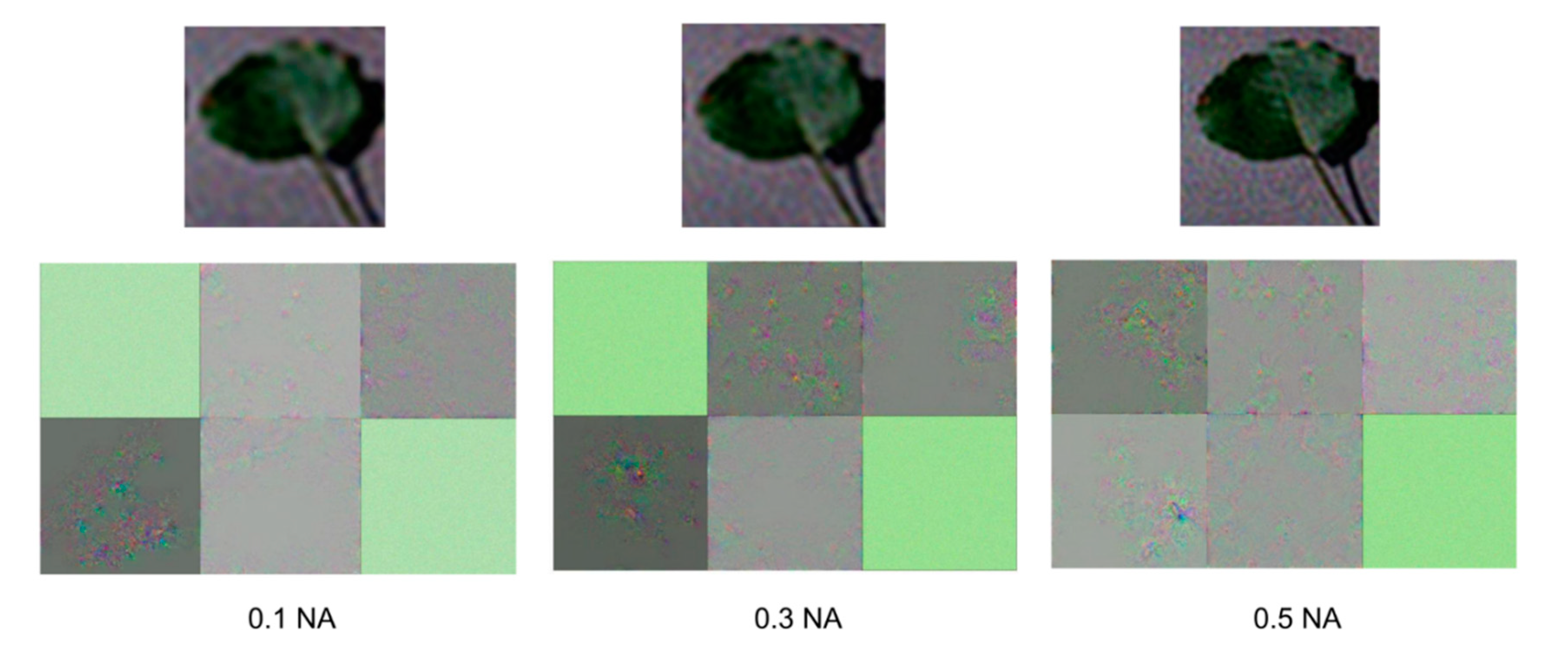
PSNR and SSIM increased with higher values of numerical aperture. For the purpose of illustrating the increased image classification accuracy due to the increase in PSNR and SSIM, the neural network activation map under different numerical apertures is presented. Figure 12 shows the Google inception convolution neural network activation map and the reconstructed images corresponding to each numerical aperture. The reconstructed image on the top of Figure 12 is the input of the Google inception neural network, and the activation map is the gradient of the features learned from the neural network.

4. Conclusions

In this study, we have investigated image classification accuracy with and without FPM reconstruction with six different image classifiers. We have also compared the image classification accuracy for the FPM reconstructed image versus the lower resolution images shown in Figure 8, Figure 9, Figure 10. It is clear that the lower resolution image has lower image visualization quality than the FPM-reconstructed image. Such a finding is further reinforced by the significant difference between the lower resolution and FPM reconstructed images in terms of image classification accuracy, especially for the lower NA conditions (e.g., 0.05 NA). For MINST, Fashion MNIST, Cifar, Caltech 101, and customized training datasets, when NA is lower, the lower resolution image classification accuracy becomes significantly lower than that of an FPM-reconstructed image. In contrast, when the image quality is higher with a higher NA condition (e.g., 0.5 NA), the image classification performance differs less significantly between with and without FPM reconstruction, which is possibly limited by classifier capabilities.

Nevertheless, the use of FPM reconstruction to improve image classification accuracy is meaningful because the lower NA image without FPM reconstruction suffers from a lower accuracy of image classification. This observation is clear across all six different datasets with different image classifiers. The catastrophic outcome is further supported by the finding that for the Caltech-101dataset, the accuracy of image classification corresponding to lower NA (0.05) and lower resolution conditions is 87% lower than the ground truth. For this situation, the use of FPM reconstruction is indeed helpful, which improves the image classification accuracy from 4.75% to 20%. Our results also suggest that the capabilities of different classifiers differ in terms of their capabilities to deal with lower NA images. The differences could be caused by different neural network structures. For example, the Google Inception Network is found to have better capabilities to retain the image classification accuracy even for the lower NA images, which is likely caused by the Inception module within the network to handle the lower resolution images.

We further built multiple linear regression between image classification value (dependent variable) and PSNR and SSIM (independent variables). Results show that there is a linear relationship between the dependent variable and independent variables (Figure 8). The related regression F-Test p-value is also smaller than 0.05, which indicates that such a linear relationship is strong. The linear relationship implies that it is feasible to predict the image classification accuracy based on the PSNR and SSIM values. The impact of noises on image classification performance has been documented in previous literature [23,24]. Specifically, Figure 12 shows the activation maps, which are the gradient features learned from the Google inception neural network. It is evident that for the low numerical aperture, which is associated with a lower SSIM and PSNR, more learned gradient features become vanished or reduced. The vanished gradient compromises the network classification accuracy. It is clear that a more vanished gradient in the learned features corresponds to the lower numerical apertures of 0.1 and 0.3, thus compromising network classification accuracy. For a 0.5 numerical aperture, the vanished gradient has been reduced, which, therefore, corresponds to the improved image classification accuracy.

This study had some limitations. First, a greater number of trials for training and the evaluation of image classification accuracy for different NAs are needed. The linear relationship between SSMI, PSNR, and image classification accuracy needs to be evaluated based on a greater number of such trials. Specifically, under extreme lower or higher NA conditions, e.g., lower than 0.05 NA or greater than 0.5 NA, an examination of the relationship is also needed. Furthermore, factors involved in the study are limited. We have not included different noises, training and testing data ratios, or a more extensive number of classifiers. We plan to address the limitations in future work.

References

- Zheng, G.; Horstmeyer, R.; Yang, C. Wide-field, high-resolution Fourier ptychographic microscopy. Nat. Photonic 2013, 7, 739–745. [Google Scholar] [CrossRef] [PubMed]
- Zheng, G.; Shen, C.; Jiang, S.; Song, P.; Yang, C. Concept, implementations and applications of Fourier ptychography. Nat. Rev. Phys. 2021, 3, 207–223. [Google Scholar] [CrossRef]
- Tian, L.; Li, X.; Ramchandran, K.; Waller, L. Multiplexed coded illumination for Fourier ptychography with an LED array microscope. Biomed. Opt. Express 2014, 5, 2376–2389. [Google Scholar] [CrossRef] [PubMed] [Green Version]
- Sun, J.; Chen, Q.; Zhang, J.; Fan, Y.; Zuo, C. Single-shot quantitative phase microscopy based on color-multiplexed Fourier ptychography. Opt. Lett. 2018, 43, 3365–3368. [Google Scholar] [CrossRef] [PubMed]
- Sun, J.; Zuo, C.; Zhang, J.; Fan, Y.; Chen, Q. High-speed Fourier ptychographic microscopy based on programmable annular illuminations. Sci. Rep. 2018, 8, 7669. [Google Scholar] [CrossRef] [PubMed] [Green Version]
- Jiang, S.; Guo, K.; Liao, J.; Zheng, G. Solving Fourier ptychographic imaging problems via neural network modeling and TensorFlow. Biomed. Opt. Express 2018, 9, 3306–3319. [Google Scholar] [CrossRef] [PubMed]
- Nguyen, T.; Xue, Y.; Li, Y.; Tian, L.; Nehmetallah, G. Deep learning approach for Fourier ptychography microscopy. Opt. Express 2018, 26, 26470–26484. [Google Scholar] [CrossRef] [PubMed] [Green Version]
- Chen, L.; Wu, Y.; Souza, A.M.D.; Abidin, A.Z.; Wismüller, A.; Xu, C. MRI tumor segmentation with densely connected 3D CNN. In Proceedings of the Medical Imaging 2018: Image Processing, (International Society for Optics and Photonics), Houston, TX, USA, 11–13 February 2018; Volume 105741F. [Google Scholar]
- Zhu, P.; Wen, L.; Bian, X.; Ling, H.; Hu, Q. Vision meets drones: A challenge. arXiv 2018, arXiv:1804.07437. [Google Scholar]
- Goyal, P.; Dollár, P.; Girshick, R.; Noordhuis, P.; Wesolowski, L.; Kyrola, A.; Tulloch, A.; Jia, Y.; He, K. Accurate, Large Minibatch SGD: Training ImageNet in 1 Hour. arXiv 2017, arXiv:1706.02677. [Google Scholar]
- Zhang, H.; Zhou, W.-J.; Liu, Y.; Leber, D.; Banerjee, P.; Basunia, M.; Poon, T.-C. Evaluation of finite difference and FFT-based solutions of the transport of intensity equation. Appl. Opt. 2017, 57, A222–A228. [Google Scholar] [CrossRef] [PubMed]
- Zhou, W.-J.; Guan, X.; Liu, F.; Yu, Y.; Zhang, H.; Poon, T.-C.; Banerjee, P.P. Phase retrieval based on transport of intensity and digital holography. Appl. Opt. 2018, 57, A229–A234. [Google Scholar] [CrossRef] [PubMed]
- Zhang, H.; Zhou, W.; Leber, D.; Hu, Z.; Yang, X.; Tsang, P.W.M.; Poon, T.-C. Development of lossy and near-lossless compression methods for wafer surface structure digital holograms. J. Micro/Nanolithogr. MEMS MOEMS 2015, 14, 41304. [Google Scholar] [CrossRef]
- Xiao, H.; Rasul, K.; Vollgraf, R. Fashion-MNIST: A novel image dataset for benchmarking machine learning algorithms. arXiv 2017, arXiv:1708.07747. [Google Scholar]
- Zhong, Z.; Zheng, L.; Kang, G.; Li, S.; Yang, Y. Random erasing data augmentation. arXiv 2017, arXiv:1708.04896. [Google Scholar] [CrossRef]
- He, K.; Zhang, X.; Ren, S.; Sun, J. Deep residual learning for image recognition. In Proceedings of the IEEE Conference on Computer Vision and Pattern Recognition, Las Vegas, NV, USA, 27–30 June 2016; pp. 770–778. [Google Scholar]
- Perez, L.; Wang, J. The effectiveness of data augmentation in image classification using deep learning. arXiv 2017, arXiv:1712.04621. [Google Scholar]
- Zhong, Z.; Zheng, L.; Zheng, Z.; Li, S.; Yang, Y. Camera Style Adaptation for Person Re-identification. In Proceedings of the 2018 IEEE/CVF Conference on Computer Vision and Pattern Recognition, Salt Lake City, UT, USA, 18–22 June 2018; pp. 5157–5166. [Google Scholar]
- Wang, R.; Song, P.; Jiang, S.; Yan, C.; Zhu, J.; Guo, C.; Bian, Z.; Wang, T.; Zheng, G. Virtual brightfield and fluorescence staining for Fourier ptychography via unsupervised deep learning. Opt. Lett. 2020, 45, 5405–5408. [Google Scholar] [CrossRef] [PubMed]
- Li, Y.; Cheng, S.; Xue, Y.; Tian, L. Displacement-agnostic coherent imaging through scatter with an interpretable deep neural network. Opt. Express 2021, 29, 2244–2257. [Google Scholar] [CrossRef] [PubMed]
- Zhang, H.; Wang, L.; Zhou, W.; Hu, Z.; Tsang, P.; Poon, T.-C. Fourier Ptychography: Effectiveness of image classification. In Proceedings of the SPIE, Melbourne, Australia, 14–17 October 2019; Volume 11205, pp. 112050G-1–112050G-8. [Google Scholar]
- Wang, L.; Song, Q.; Zhang, H.; Yuan, C.; Poon, T.-C. Optical scanning Fourier ptychographic microscopy. Appl. Opt. 2021, 60, A243–A249. [Google Scholar] [CrossRef] [PubMed]
- Gowdra, N.; Sinha, R.; MacDonell, S. Examining convolutional feature extraction using Maximum Entropy (ME) and Signal-to-Noise Ratio (SNR) for image classification. In Proceedings of the IECON 2020 the 46th Annual Conference of the IEEE Industrial Electronics Society, Singapore, 18–22 October 2020; pp. 471–476. [Google Scholar]
- Li, Q.; Shen, L.; Guo, S.; Lai, Z. Wavelet Integrated CNNs for Noise-Robust Image Classification. In Proceedings of the IEEE/CVF Conference on Computer Vision and Pattern Recognition (CVPR), Seattle, WA, USA, 14–19 June 2020; pp. 7245–7254. [Google Scholar]
Figure 1.
The iteration process of FPM. In the iteration, the sampling rate of the initial guess of the high-resolution object is higher than the collected low-resolution images. Through the iterative process, the reconstructed image is increased in spatial resolution.
Figure 2.
Convolution neural network architecture for image classification using MNIST data.
Figure 3.
Convolution neural network architecture for image classification using Fashion-MNIST data.
Figure 4.
Residual convolution neural network architecture for image classification using the CIFAR dataset. The line (on the right side) in the residual layer represents a skipped connection.
Figure 5.
Residual convolution neural network architecture for image classification training using the Caltech 101 dataset. Res2s_branch2a represents the second stage and the second branch.
Figure 6.
SqueezeNet convolution neural network architecture for image classification training using the flowers dataset. Fire2_squeeze means the second stage squeeze module.
Figure 7.
Google inception convolution neural network architecture for image classification training using the apple pathology dataset. Conv2_3 × 3 represents the second stage, 3 × 3 convolution filter.
Figure 8.
(A) Lower resolution MNIST image; (B) FPM reconstructed MNIST image; (C) original MNIST image; (D) lower resolution Fashion MNIST image; (E) FPM reconstructed fashion MNIST image; (F) original Fashion MNIST image.
Figure 9.
(A) Lower resolution CalTech 101 image, (B) FPM reconstructed CalTech 101 image (C) Original CalTech 101 image (D) Lower resolution Fashion CIFAR image (E) FPM reconstructed CIFAR image (F) original CIFAR image.
Figure 10.
(A) Lower resolution apple pathology image; (B) FPM-reconstructed apple pathology image; (C) original apple pathology image; (D) lower resolution flowers image; (E) FPM-reconstructed flowers image; (F) original flowers image.
Figure 11.
Visualization of data distribution for multiple linear regression between image classification accuracy, PSNR, and SSIM.
Figure 12.
Visualization of the apple pathology images and Google inception convolution neural network activation map (gradient) at the 141st layer. In total, the Google inception convolution neural network had 144 layers. The 141st layer is followed by the fully connected layer, the softmax layer, and the output layer. The green color corresponds to the vanished gradient. Fewer features in the activation map corresponds to the reduction in gradient.