
Technological Development and Application of Photo and Video Theodolites


1
Department of Applied Geodesy, Faculty of Geodesy, University of Zagreb, Kačićeva 26, 10000 Zagreb, Croatia
2
Department of Photogrammetry, Plc., Borongajska Cesta 71, 10000 Zagreb, Croatia
*
Author to whom correspondence should be addressed.
Appl. Sci. 2021, 11(9), 3893; https://doi.org/10.3390/app11093893
Submission received: 26 March 2021
/
Revised: 22 April 2021
/
Accepted: 22 April 2021
/
Published: 25 April 2021
(This article belongs to the Special Issue Analyses in Geomatics: Processing Spatial Data on History and Today)
Abstract
:Theodolites are fundamental geodetic measuring instruments for all practical geodetic tasks, as well as for experimental geodetic scientific purposes. Their development has a long history. Photo and video theodolites represent the advanced development of classic theodolites. Development started in 19th century, but only in the last 15 years has commercial application been achieved in the geodetic profession. The latest development, called image-assisted total stations (IATS), is a theodolite which consists of a classic robotic total station (RTS) with integrated image sensors. It was introduced in the early 2000s. With the development of theodolites, their application became much wider; today, they can be used for structural and geo-monitoring, i.e., for the determination of static and dynamic displacements and deformations of civil engineering structures such as bridges, dams, wind turbines, and high buildings, as well as natural structures, such as mountain slopes. They can be implemented in geodetic monitoring systems, which are an integral part of engineering structural diagnosis, and they provide essential information about the current condition of the structure. This paper describes the technological development of photo and video theodolites divided into phases according to the main innovations in their development. The application of modern video theodolites (i.e., IATS) is presented through several experimental studies that were performed. The procedure of conducting measurements with this kind of instrument, as well as the analysis of acquired data and achieved results, is elaborated. Lastly, the authors conclude, according to the achieved results, that IATS can today be used for determination of quasi-static and dynamic displacements with small and high amplitudes.
1. Introduction
A theodolite is a geodetic instrument for measuring horizontal and vertical directions, i.e., angles in the horizontal and vertical plane. There are optical and electronic theodolites [1,2,3]. To determine the point positions in the coordinate system, in addition to angles, we must measure the distance between the instrument and the target. We can measure the distances mechanically (with chains and measuring tapes), optically (with optical distance-meters and interferometers), and electronically (with electro-optical distance-meters and electronic distance-meters (EDMs)). The accuracy of mechanically and optically measured distances is low and not appropriate for terrain characteristic point coordinate calculations. With time, several technological developments have been incorporated into theodolites; thus, the accuracy of angle and distance determination has significantly increased. Perhaps the biggest development of theodolites was its integration with an electronic distance-meter (EDM), which emerged around 1940 and became commercially available in the late 1960s [4]. The type of EDM incorporated into modern total station instruments is commonly of the electro-optical type, using infrared and laser light as a carrier signal [3]. Instruments which can measure angles and distances simultaneously, as well as record the results and, to a certain extent, process them, are called electronic tachymeters or total stations (TS) [2]. TS instruments are electronic digital theodolites integrated with EDM instruments and electronic data collectors, which are aimed at replacing manual field data recording; they are capable of providing electronic angle readings, as well as distance measurements [3].
Today, many different sensors and measurement methods are combined in TS, such as highly accurate angle reading, electronic distance measurements (EDM) to reflectors and to any other surface (reflectorless EDM), tilt correction by two-axis inclinometers, different types of motorization to drive both the horizontal and the vertical motion of the instruments, servo, piezo, and magnetic motors (robotic total station—RTS), image CCD (charge-coupled device) or CMOS (complementary metal–oxide–semiconductor) sensors (CCD or CMOS) for autofocus, automated aiming (i.e., automatic target recognition (ATR) and tracking of signal points), integration with global navigation satellite system (GNSS) positioning, wireless communication and operation using a controller, additional cameras for documentation (image-assisted total station—IATS), and IATS with a scanning function (image-assisted scanning total station—IASTS). Due to the rapid hardware development, as can be seen in Figure 1, these different sensor classes, each with their specific advantages, can be unified, utilized, and are fused as one single (nearly) universal instrument [5]. Modern TS are multi-sensor systems which can determine the three-dimensional coordinates of target points by combining horizontal angle, vertical angle, and distance measurements [6].
Figure 1 shows the technological development of TS over the years, i.e., from the mid-20th century until today. The main hardware and software, sensor integration, and their impact on instrument performances and operator efficiency for conducting the measurements in the field are shown. It is evident that, following the integration of EDM with the basic theodolite in the 1960s upon discovering tachymeters, the dimensions and weight of the instruments decreased, as well as the expert efficiency regarding the measuring techniques and time for conducting measurements in the field. Contrarily, instrument performance and the possibilities for surveying and monitoring projects have rapidly increased.
Different types of motorization developed to drive instruments in horizontal and vertical motion have been specially designed and implemented in RTS to automatically search for reflectors and, later, for reflector tracking. Most commonly, RTS are used for highly precise measurements such as displacements and deformation monitoring of civil engineering structures and the Earth’s surface.
RTS with additional integrated cameras in the telescope are commonly denoted as image-assisted total station (IATS) [7]. In the literature, a number of alternative terms exist for this class of instruments [8]: photo theodolite, video theodolite/tacheometer, image-assisted photogrammetric scanning station, and others. Differentiation is often made between a video and an image or photo. This fact was valid in the past, considering analog imaging devices introduced at the end of 19th century. Static instruments on a leveled, rotatable platform with the main function of taking images using a photogrammetric camera, supported by a theodolite for determining the elements of the exterior orientation, are called photo theodolites [9,10].
Currently, IATS have possible applications in semiautomated object reconstruction systems [11], fully automated deformation monitoring systems [12], industrial measurement systems [13], measurements of vibration amplitudes by means of high-frequency image measurements [14], capture of additional information such as high-frequency motions or intensity fluctuations of patterns using image sensor to derive the temperature gradient of the atmosphere as a decisive influence parameter for angular refraction effects [15] and monitoring of cracks [14,16].
This study reviews and describes the technological development of photo and video theodolites divided into phases according to the main innovations in their development (Section 2). Emphasis is placed on commercially developed instruments; however, prototypes from academia are also analyzed, since they often inspire technological developments. The basic principles of the modern IATS, camera and system calibration, and measurement procedures and data processing approaches are explained (Section 3). The application of IATS, as the successor to photo and video theodolites, is presented through experimental and in situ studies previously performed (Section 4). Lastly, a discussion with the main conclusions from conducted studies is presented.
2. Technological Development
We can differentiate two main phases in the development of photo and video theodolites. The first phase is considered when the theodolite was a supporting tool for photogrammetric cameras, called photo theodolites, and the second phase is considered when the camera became a supporting tool for theodolites, i.e., tachymeters and total stations, called video theodolites.
The second phase involving the technological development of video theodolites can be divided into four main phases according to the main innovations in their development. In this section, each phase is described, and the main innovations are explained.
2.1. Development until 1940
Photo theodolites have been known for more than 150 years in photogrammetry. The main credit for the introduction of photogrammetry goes to Aime Laussedat, an officer in the Engineer Corps of the French Army. He is known as the “Father of Photogrammetry” as he constructed the first usable cameras for terrestrial work in 1851 [17]. He generated the first maps by means of photographs which he took from a balloon. His remaining research focused on terrestrial photogrammetry, designing the first photo theodolite which consisted of a camera and theodolite [18]. The end of 19th century was significant for the development of terrestrial photogrammetry, which was applied in many mapping projects. In 1889, the Italian army developed the photo theodolite (Figure 2, left). Sebastian Finsterwalder, in 1899, wrote his dissertation on the “fundamental geometry of photogrammetry”, in which he solved the problem of determining the position of two camera stations, i.e., stereopairs, independently of terrain measurements from four points identified on both photographs, as well as the methods of relative and absolute orientation. He also developed his own photo theodolite (Figure 2, middle). German Carl Pulfrich, with the construction of his photo theodolite (Figure 2, right), designed the first modern stereo comparator which used the principles of stereophotogrammetry and x–y coordinate scales [17,18]. At first, a photogrammetric camera was combined with components such as an aiming device, pitch circle, level, and tripod [19].
The Wild company in 1922 constructed the first commercial photo theodolite, Wild P30 (Figure 3, left) [20]. The instrument was a combination of a camera and theodolite and, as such, was unique in the world. Wild’s phototheodolite was the most accurate over the next three decades. The magnification of the telescope was 28×, and the direction reading with an optical micrometer was 1”. The focal length of the camera lens was 165 mm. The camera and the theodolite weighed 27.5 kg, while the weight of the complete measuring equipment with all the necessary aids was about 65 kg. The instrument was applicable to all large and small geodetic tasks. The instrument’s reliability during field work in the most difficult conditions, which are common during surveys in high mountains, was one of its main advantages. Three years later, Wild introduced a new model of photo theodolite called the Wild FT9 (Figure 3, right). The mechanical construction of the theodolite and the camera simplified the determination of the camera’s orientation for photogrammetric postprocessing.
2.2. Development from 1941–1980
After World War II, a theodolite named Electronic Eye (Figure 4, left) was developed at the Institute of Applied Geodesy in Frankfurt for automated aiming based on the difference of two currents in a photoelectric cell. This method was further developed to enable bearing accuracies of 1” as a mean of six sets of directions in the late 1950s [21]. Testing gave very good results; thus, the company Askania produced a modified theodolite based on Electronic Eye—the Askania Tracking System (Figure 4, right).
While Electronic Eye could only measure static targets, the Askania Tracking System already had the ability to register the orbit of moving objects (aircraft or missile) during WW2. The Askania Tracking System was used as a tracking system from the late 1950s to 1973 [23]. Later, the type of theodolite shown on the left of Figure began to be produced in Switzerland under the name Contraves EOTS (electro-optical tracking system) and was later produced in China [22]. The instrument, called a cinetheodolite, was used to record important data during testing of missiles and aircrafts, as well as other experimental weapon systems. Ballistic cameras that were used in satellite geodesy very often had integrated CCD image sensors for video recording, and they can also be structurally considered as video theodolites [22].
With the aim of recording the landing of aircraft using the instrument, in 1972, a portable Minilir system was developed in Paris [22]. The system was developed as part of the internal research project SAT (Société Anonyme de Télécommunications), and it was not only a geodetic advancement but also a military tool for automatic monitoring of infrared radiation, such as aircraft and missile exhausts. The aiming was based on the detection of aircraft headlights using a very sensitive infrared sensor that recorded the frequency and phase-modulated signal. This instrument has been used since the 1980s in combination with various distance-meters such as the IBEO Fennel electronic distance-meter (EDM) or the AGA Geodimeter-112 EDM. Depending on which EDM was in place, the instrument was referred to as AGA-Minilir (Figure 5, middle) or Fennel-Minilir. This instrument was used as early as 1980 in the Dutch delta project for the coastal navigation of transport ships. In combination with a film camera, the system became known as a cinetheodolite, which was used on launch sites Kourou (Guiana Space Centre) and Cape Canaveral. In civil use, Minilir has been used for the calibration of instrument landing systems [24].
Minilir was followed, in 1983, by the Krupp Atlas-Elektronik instrument known as Polarfix (Figure 5, right). The laser measuring principle for short-range high-accuracy dynamic survey applications was the basis of Polarfix. Polarfix had several advantages and improvements compared to the Minilir system. While Minilir required a heat source to find the target, Polarfix only needed a passive reflective prism to achieve target tracking. The vertical circuit was automatically compensated for, and the instrument could be operated on a 12 V source instead of a 220 V source, which allowed the use of batteries. Its weight and volume were twofold lower compared to Minilir. The system provided polar coordinates for position fixing, incorporated a fully automatic operator-free tracking function, and ensured range/azimuth fixing to 10 cm + 5 cm/km accuracy from a single shore-station linked to shipborne telemetry and beam reflector facilities. The operating range depended on weather and other factors, but its typical basic range was just under 3 km, which could be extended to 5 km or more. This instrument was primarily designed for tracking ships on inland waterways [25]. The 1970s and 1980s were marked by the integration of EDM and electronics in general into theodolites, which also influenced the introduction of a new name for such instruments, i.e., electronic theodolites or electronic tachymeters (ETs) [26].
2.3. Development from 1981–1990
Development during the 1980s placement emphasis on theodolite measurement systems (TMSs). ETs combined with integrated cameras, i.e., image CCD sensors, were used to measure spatial forward intersections using two or more instruments. The automatic aiming at fixed target points or projected laser spots was realized using image analysis techniques [8]. Most of these devices were used for industrial applications.
In 1981, the Geodetic Institute of the University of Hannover took up the idea of using four-quadrant diodes as part of the Collaborative Research Center 149 within a subproject called “automatic determination of the position of an object at sea using a tachymeter”. A semiconductor position-sensitive sensor built into the image plane of a tachymeter was used to detect the center of the light source located on a monitored ship. With the help of built-in servomotors, the instrument could monitor the ship, always keeping the light source in the middle of the field of view (FOV). This development was based on the AGA Geodimeter 700, which had infinite screws for fine adjustment, named GEOROBOT, and GEOROBOT II was later developed on the basis of the Geodimeter 710 instrument [27,28].
Two instruments which marked this period were presented at almost the same time, i.e., Kern E2-SE (Figure 6, left) introduced in 1985 [29] and Wild TM-3000V (Figure 6, right) introduced shortly after [30]. These instruments were developed through projects from Kern and Wild and were actually called Kern SPACE and Wild ATMS during the project phase. The growing demands of manufacturers in the automotive and aerospace industries, who used theodolite measurement systems during assembly and quality control, were based on measuring spatial forward intersections using two or more instruments. To satisfy these demands, Kern and Wild integrated CCD image sensors and digital image acquisition into servomotorized theodolites. These so-called video theodolites had pan-focal telescopes, which means that the FOV changed as a function of distance to the target point. Kern E2-SE had a CCD image sensor with a resolution of 576 × 684 px, and the image was recorded in the instrument’s internal memory. It was the first video theodolite in the world with the possibility of automatically aiming at a signaled target [2]. The CCD image sensor was used for autofocusing and for determining the target position relative to the optical axis of the telescope. The instrument had three integrated servomotors, two for horizontal and vertical axes and one for focusing, i.e., autofocus. The motors were designed to enable a positioning accuracy of up to ±0.1” to be achieved, at speeds of up to 54° per second [31]. Once the autofocus was accomplished and the geometrical relationship between the target point and the instrument optical axis was determined using image processing algorithms, the instruments automatically drove the theodolite toward the target point and the measurements could be performed. A signaled target point realized by a projected laser point or a fixed marking was automatically aimed at by two or more corresponding instruments using image evaluation, allowing its 3D spatial coordinates to be determined [22].
Shortly after Kern, the Wild company introduced its video theodolite model TM3000V. The motorized video theodolite TM3000V was a further development of the precision theodolite T3000. In addition to the motors for the axes and the focusing lens, special elements of the motorized video theodolite were the camera and the processor integrated in the theodolite. Wild TM3000V had a CCD image sensor with a resolution of 500 × 582 px. The coaxial configuration of a camera (integrated into the telescope) using theodolite optics was better, but also technically more complicated than biaxial implementation onto the telescope leading to parallax, which is particularly harmful in situations where range-finders operate at close target distances. When using the coaxial configuration, complex beam splitter elements must be installed. The Leica TM3000V video theodolite is the best-performing example, widely used in academic research [11]. The image of the FOV of the telescope on the CCD array contains the image of the targeted point, as well as a reference frame built into the telescope to replace the reticle. This frame defines the target line of the telescope with the center of the lens system, and it is used at the same time to adjust the telescope and camera axis. Using the CCD camera, a wide-angle lens can initially be used to display an overview image of the object space with a size of 9° × 12°. These wide-angle optics can be exchanged for the optics of a precision telescope via an optics coupler. Instead of the wide-angle FOV, however, a narrowly limited measuring FOV is available. Switching between the measuring and wide-angle FOV is controlled by the software. Switching to the measuring FOV enables high increases in accuracy, since details of objects that are far away are now displayed on the entire sensor surface.
These instruments were only used for special applications and not for standard surveys due to their complex morphology, which required an image display unit and a control unit in addition to the instrument [32]. With the launch of laser tracker systems in the 1990s, video theodolites were replaced within a few years; this remained a trend until 2005, when Topcon introduced the first commercially known IATS model GPT-7000i, which was the forerunner of today’s state-of-the-art IATS. However, technical innovations that were necessary for automation using video images and were, therefore, introduced on the market have been preserved to this day, for example, the motorized endless fine drives for instrument control, as well as reflector detection and tracking using integrated image sensors, which are common today, from the second generation of the Wild TM3000V. As in the TOPOMAT project, a target illuminator in the form of an infrared collimator was installed here for permanent deformation measurement on reflectors. This diode integrated in the telescope illuminated the roughly approached reflector. The reflected signal was captured on the infrared sensitive CCD array and used for precise targeting [30].
The concept involving the difference of two currents in a photoelectric cell, named “Electronic Eye”, become commercially available in 1987 when Geodimeter presented the model 4000 “One-Man-System” with automated target aiming, being the first instrument that required only one expert to operate it (Figure 7) [22]. Since then, automated target aiming and tracking have become standard functions in all TS, i.e., RTS. Integrated cameras and photogrammetric methods became supporting tools for theodolites. This system worked using a theodolite-like active target point receiver, whereby the telescope of this unit, called the remote processing unit (RPU), had to be aligned with the total station, called the control and processing unit (CPU), in order to facilitate a coarse search.
2.4. Development from 1991–2000
Available prototypes of video theodolites (Figure 6) in the 1990s encouraged intensive research on their application with high degrees of automation. Equipped with motors, video theodolites made it possible to increase the dynamism of computer-controlled measurements, turning a video theodolite into a robot [33]. Built-in sensors provided a wealth of data that demanded to be processed meaningfully to obtain the necessary information. Electronic reading of directions and lengths was around for a long time, but the processing of data obtained using built-in cameras was still in its initial stages. The application of digital image processing methods and computer vision was investigated by the academic community. Initial research focused on detecting artificial targets and accurate aiming with the help of cameras [34].
Aiming at and measuring unsignalized targets proved to be a special challenge [35]. To achieve this, solutions based on artificial intelligence were developed [36]. Until then, the expert/operator was in charge of sighting and deciding on the characteristic points to be measured. By implementing this knowledge into software solutions, artificial intelligence was applied, and expert systems were developed. Initially, development was limited to smaller and simpler processes that occurred in theodolite measurements [37]. Special attention was paid to the necessary sharpening of the image by developing autofocus algorithms [35,37].
The developed processes and procedures were later implemented in commercial solutions of instrument manufacturers. This freed observers from repetitive operations, whereby they could now focus on more complex tasks. By automating the measurements, the level of achieved accuracy was increased. Computer-aided measurements and data processing provided greater accuracy than could be achieved visually by the observer. The developed systems could be applied to measurements in the industry. It was no longer necessary to bring the object to the measurement place since the system could be transported. External control of the developed systems allowed measuring objects at hazardous places. Since unsignalized targets could be targeted, measuring of inaccessible objects also became possible.
At the very beginning of this epoch, in 1991, the automatic measuring system TOPOMAT was developed in Zurich. In collaboration with Wild, it was upgraded with a CCD image sensor to detect the target [22]. Its main features were that it could work independently, automatically, or via a controller. Other functions were also available via the controller, such as activation, deactivation, and change of measurement method [38]. GEOROBOT and TOPOMAT had encouraged the development of commercial tracking TS.
The transition from the 1980s to the 1990s was also marked by the development of the ATR function, which enabled the further development of IATS instruments. In 1991, Topcon presented its first motorized, auto-tracking total station AP-S1. In 1993, Topcon released its successor called model AP-L1, and 1996 saw the emergence of the new model AP-L1A, the so-called “one-person surveying system” [39]. This RTS differed from the instruments and developments presented before in that the fine aiming, similar to the structure of a television image, worked with line-deflecting optical elements (AO device) and could, thus, evaluate an image of the reflector illuminated by the instrument [40]. This system worked in conjunction with radio communication, a handheld data collector, and TDS Survey Pro Software. It produced a unique surveying system that enabled all field surveying tasks to be carried out by one expert working on their own.
The Wild company, i.e., Leica, from the beginning of the 1990s presented its first motorized self-aiming surveying system with an automatic target recognition function that worked without an external evaluation unit in 1996, i.e., the model TCA1800. This system also worked with an imaging CCD sensor and evaluated the illuminated image of the reflector using a best-fit algorithm. With this instrument, a new type of compact 360° all-round reflector was developed [22].
2.5. Development from 2001 until Today
The forerunner of today’s state-of-the-art commercial IATS systems was Topcon’s model GPT-7000i from 2005 (Figure 8). Topcon integrated the camera into a TS, which created a new generation of video theodolites, named IATS. The instrument was equipped with two different VGA cameras. One camera was wide-angle with an FOV of 28° × 22° and fixed focus, located on the telescope, allowing rotation to be synchronized and the field working area to be displayed. The second camera was coaxial, and it recorded the details of the terrain seen through the magnification of the telescope; thus, it included variable focus. It had an FOV that matched the telescope FOV (1°30′ × 1°30′) [41]. In 2007, Topcon introduced the successor of the first series model GPT-9000Ai. The greatest technological development compared to the GPT-7000i was manifested as the possibility of automatic focusing of signal points and remote guidance by the controller, which eliminated the need for an observer, making it a so-called “one-man station”. It was also the first RTS that enabled the taking of photographs and the possibility of scanning as a unique function within the IATS system. The instrument could scan up 20 points per second [42]. These types of IATS have been produced by Topcon for three generations and are known as Imaging Stations, with the latest model called IS3. Both cameras had an image sensor with a resolution of 1280 × 1024 pixels, and they could also record video at 10 frames per second (fps), which could be transmitted to the station control screen or to the controller screen.
Trimble introduced its first IATS in 2007, the model VX Spatial Station (Figure 8). It was basically an S6 model with added functionality of 3D scanning and digital imaging. VX delivered images that were accurately georeferenced. The instrument was equipped with a 3 MPx color camera, with fixed focus and an FOV of 16.5° × 12.3°. The camera was located on the telescope. This camera was later implemented in all total station models that Trimble released, including today’s Trimble S9 series. The features of postprocessing photogrammetric analysis of calibrated images, 5 fps video recording, panoramic mosaic image, and overlap with measured data are known as “Trimble Vision”. The VX Spatial Station was an RTS with MagDrive servo technology, involving an integrated servo/angle sensor electromagnetic direct drive in combination with added digital imaging and rudimentary scanning capabilities. The scanning function could scan 20 points per second with the ability to colorize scanned scenes based on recorded images [43].
In 2009, Pentax presented an RTS with integrated cameras into its instruments, known as Visio series model R-400VDN. The camera was placed on the telescope, and a screen displaying captured images and video from the camera was also placed on the telescope above the ocular (Figure 8). The FOV was 8.8° × 8.8°, and it could record video at 10 fps [44].
Leica introduced its IATS instrument in 2010 called Viva; two models with overview cameras placed on the telescope were presented: Leica TS11 and Leica TS15 (Figure 8). Model TS15 was motorized using a servofocus drive with additional sensors for automatic and remote control, unlike TS11. The overview camera had an optical axis different from the optical axis of the telescope, which resulted in parallax; thus, the center of the optical axis of the telescope did not coincide with the center of the image sensor. The relative position of these two axes was determined by calibration at the time of its manufacturing. The effect of parallax could also be corrected by measuring the distance to the target. The integrated cameras in both models had a 5 MPx CMOS image sensor, with fixed focus and an FOV of 15.5° × 11.7°, with the possibility of recording video at 20 fps [45,46].
It should also be mentioned that, at the beginning of this commercial period when IATS systems were brought to the geodetic scene, the first IATS instrument was actually presented by Sokkia (SET3110MV) at INTERGEO 2002. The instrument had two integrated cameras, an overview camera on the telescope and another camera integrated in the telescope. The curious aspect of this instrument was that it did not have an ocular; instead, the expert performed measurements using a remote controller displaying the live video obtained from the integrated cameras.
In 2013, Leica introduced the new series called Nova with two models TS50 and MS50. The instruments, in addition to an overview camera, had an integrated camera in the telescope with an FOV of 1.3° × 1.0°, an 8× digital zoom of the overview camera, and a 30× optical zoom of the telescope camera, as well as an 8× digital zoom. That way, the images from the telescope camera were magnified 30×. Leica MS50 also had a scanning function with the ability to scan 1000 points per second. Leica TS50 did not have a scanning function. Both models used the same motorization using a servofocus drive. On the basis of the scanning function with video and photo capture capabilities, a combined approach to image analysis and scanning was developed [47,48]. In 2015, Trimble introduced its state-of-the-art IATS model S9 which used the same camera and image sensor as Trimble VX Spatial Station introduced in 2007. However, the S9 comes in at least 10 different possible configurations. The S9 replaced the VX and S8 for both precise and long-range applications. It offered higher angular and distance accuracy than the VX Spatial Station [49]. The predecessor of today’s state-of-the-art IATS and IASTS company, Topcon, unfortunately abandoned its original design with two integrated cameras in the instrument; in 2014, it offered IATS model DS-200i with one camera, an overview ultra-wide camera on the telescope with a 5 MPx image sensor, which was mainly integrated for providing imaging documentation and a live video stream on the remote controller [50].
In Table 1, Leica TS60, Trimble S9, and Topcon DS-200i are compared with their main specifications and characteristics. These instruments do not offer a scanning function as they are classified as total stations not multi-stations, although S9 offers a combined model with a scanning function.
Today, Leica offers the models TS60 and MS60 from the Nova series introduced for the first time in 2015 with improved functions of ATR (ATR plus), reflector self-search using the PowerSearch function, dynamic look function, motorized direct drives based on Piezo technology, improved scanning function with 3D laser scanning of 30,000 points per second, image-assisted surveying, and documentation using advanced artificial intelligence; it is called the first self-learning multi-station [51].
Trimble introduced its new generation of IATS instruments in 2016, model SX10. This is the first commercial TS, i.e., IATS without an ocular. Three 5 MPx cameras (overview, primary, and general) are integrated in the telescope, offering a maximum total FOV of 360° × 300° with 84× zoom. The general camera enables an FOV of 57.5° × 43.0°. An expert controls the instrument using a remote controller via live video at 15 fps. SX10 combines high-density 3D scan data, enhanced imaging called Trimble Vision, and high-accuracy total station data. It uses MagDrive servo technology, and it can measure dense 3D scan data at up to 26,600 points per second with high precision over the full measurement range of up to 600 m [52]. There was some confusion, even among Trimble developers, as to whether it should be considered a new scanner or a new total station. However, it is still classified as a TS because of its characteristics regarding the telescope, angle and distance measurements, and the possibility to measure explicitly one point. Since it combines imaging with scanning on a level that is not rudimentary, we can call it the first image-assisted scanning total station (IASTS). At the beginning of this year, Trimble introduced its successor SX12. The technical data offered at the moment describe the following upgrades: 8.1 MPx image sensors, 107× zoom of the main camera, and a new laser pointer, while the remaining features regarding angle and distance measurements and scanning function are at the same level as SX10 [53].
Topcon presented its IASTS GTL-1000 in 2019, and it is the world’s first RTS and laser scanner with an inbuilt camera, which is primarily used for colorizing the scanned scenes. The camera has a 5 MPx image sensor which is also used for live video. A 3D laser scanner is installed in place of the RTS handle, resulting in a solution that it is both a geodetic measuring station and a geodetic 3D laser scanner. The instrument uses direct drive via an ultrasonic motor. The main advantage of this IASTS compared to other commercially available IASTS is the scan rate, which is on the level of today’s terrestrial laser scanners and is specified as 100,000 points per second. It is the first such instrument in the world [54].
In Table 2, Leica MS60, Trimble SX12, and Topcon GTL-1000 are compared with their main specifications and characteristics. All instruments have a scanning function and they are classified as multi-stations, so-called IASTS. These three instruments, at the moment, represent the state-of-the-art geodetic instruments in the world.
All currently available commercial IATS and IASTS instruments use recorded images and videos for additional attributes of the measured point, i.e., primarily for documentation and colorizing the scanned scenes. Standard measurement methods in the field have been largely developed and improved by technological developments of TS. Manual focusing has been replaced by auto-focusing; moreover, using remote control, an expert can select the point of interest defined by a pixel from a live video/image on a display, thereby pointing the instrument to a signalized or unsignalized point. For pointing the instrument to the point of interest and for tracking the reflector in the field, instruments use motorization, which is currently realized by piezo, magnetic, or ultrasonic drives depending on the manufacturer. The recorded images can be automatically downloaded for each point or for a set of points for documentation purposes. This way, it is possible to visualize these points. More importantly, we can perform photogrammetric processing of collected georeferenced images afterward and, e.g., use them for structural and geo-monitoring, leveling, and fusion of laser scan and image data for deformation monitoring. However, commercial IATS and IASTS instruments still do not use the full potential and functions of these instruments [8]. In the next section, the potential for application of the latest state-of-the-art IATS is presented.
3. Measurement and Processing Approaches
Depending on the developed hardware and software, integrated sensors, and different functions through the implementation of various algorithms in TS, we can distinguish types of TS (Table 3).
State-of-the-art IATS and IASTS represent a new kind of RTS, unifying the geodetic precision of TS with the areal coverage of images, as well as laser scans. IATS offer the user an image-capturing system with integrated camera(s) using image sensor(s) in addition to a polar 3D point measurement system. IASTS are equipped with a scanning function with lower scan rates comparable to classical terrestrial laser scanners. The greatest advantage of using such a (multi-sensor) instrument is the common coordinate system of all built-in sensors, as long as appropriate a priori calibration is provided [55].
These multi-sensor systems can capture images for documentation and for photogrammetric measurements. They can even merge more of these captured images into a panoramic image mosaic using camera rotation, i.e., telescope rotation. With appropriate calibration, these images are accurately georeferenced and oriented, such that they can be immediately used for direction measurements with no need for object control points or further photogrammetric orientation processes [15].
3.1. IATS Basic Principles
The combination of cameras with image sensors and theodolites was described long ago by [29,56]. In this section, we explain the basic working principles of state-of-the-art IATS Leica MS50, which are also applicable to MS60 and other IATS produced by manufacturers with two cameras (overview and telescope). Overview and telescope cameras offer the possibility to record high-resolution images or panoramic image mosaics, which can be directly linked and referenced to the 3D point measurement system. These images can be used for field documentation and, most importantly, for a posteriori photogrammetric processing. The photogrammetric resolution of 1 px of the telescope camera corresponds to 5 cc, which results in a resolution of 2 mm at 200 m [57]. The expert uses the overview camera for roughly aiming at the target, signalized or unsignalized. The overview camera image gives an overview of the surveying area; alternatively, a live video can be observed on instrument display. Using the telescope camera, which is located on the optical axis, a telescope magnification of 30× is at the expert’s disposal for very precise target aiming (Figure 9).
The achievable accuracy of angular measurements using this camera is 1”. Using the integrated image sensor, single autofocus and continuous autofocus functions are possible. Integration of the image sensor is done in such way that a focused image is simultaneously visible on the instrument display and on the instrument optical path through the ocular. A Porro prism reflects the incoming light through the telescope optics onto the imaging CMOS sensor and directly onto the ocular for visual aiming if needed. The focusing module production guarantees a 1” angular measurement accuracy. Adjustment and calibration processes are key factors to achieve the highest quality of the imaging functionality.
Prior to the available IATS, there were RTS, which, with implemented ATR functions, are also IATS in the narrowest sense since image sensors or segmented photodiodes are used for signal target detection and aiming. However, these image sensors could not be used for image documentation and photogrammetric measurements because the expert did not have access to the images and because only the light in the spectrum measurement signal was detected by imaging sensors or photodiodes [58]. The difference today is evident in the way in which the expert extracts the information from the integrated camera, i.e., from a single image (point of time) or from a video (sequence of images). We can also distinguish static or kinematic processes. With modern digital imaging sensors, both measuring tasks are possible and no differentiation of the instrument is necessary [8].
3.2. IATS System and Camera Calibration
The use of an appropriately calibrated camera is of crucial importance for displacement monitoring. It allows a two-dimensional image coordinate to be presented in angular units, i.e., field angle in the object space, which can then be expressed in linear units. All intrinsic and extrinsic parameters must be known for each captured image, which means that the images are directly georeferenced. They can be used for displacement monitoring with no need for object control points or further photogrammetric orientation processes. Photogrammetric image measurement methods, in order to detect signalized and unsignalized targets, can be combined with functions of the TS to generate precise angle and distance measurements [8].
In this section, we explain the camera calibration placed in the IATS telescope, i.e., in the optical path of the telescope. We focus on this camera and not the overview camera, because it is better to use the telescope camera for the purpose of displacement monitoring since we need highly accurate data for the determination of dynamic displacements with high speed and small amplitudes. Highly accurate data can be obtained using a telescope camera, because it uses telescope optics and magnification; however, we must also perform camera calibration, which involves the determination of intrinsic camera parameters. The intersection of the optical axis with the image sensor plane, i.e., principal point image coordinates, the focal length in the horizontal and vertical directions, and an arbitrary number of coefficients to compensate for radial and tangential lens distortions are intrinsic parameters which must be determined during camera calibration [59]. The distance between the camera center and the principal point is the focal length of pinhole cameras integrated in today’s IATS. Two focal lengths (horizontal and vertical) must be determined because the pixels on the image sensor are non-square for some cameras [60]. Imperfect manufacturing of the lens and defects in the assembling of the camera result in radial and tangential lens distortions of the linear model for projecting points in the real world to the image plane [60].
Since monitoring assumes measurements between two or more different series or epochs of point measurements, the constant image coordinates of the principal point are void and, for this reason, they do not need to be known in advance. The distortion effects exhibit a spatial regularity, such that neighboring pixels are affected similarly. Thus, distortion effects are reduced to an insignificant extent when computing differences between objects located in similar regions on the image sensor. The frequencies included in a time series, which can be computed via Fourier analysis, are independent of the physical unit of the time series. This is due to the linear property of the Fourier transform (Equation (1)), where a constant factor c may be applied before or after the transformation [59].
The frequencies of structure vibrations can be computed from the raw image coordinates, i.e., from the image coordinates of measured points. Thus, no camera calibration is needed for this purpose. To present the displacements obtained from two epochs of measurement in linear units (e.g., m, dm, cm, or mm), the camera’s angular resolution must be known. The displacements on the image are determined in pixels and can be computed as angular quantities, which can then be presented as linear units when the measured distance from the instrument to the monitored object is known. The angular resolution expresses the size of one pixel of the image sensor as an angular unit. It presents the angle between two objects that are presented on two neighboring pixels. For a pinhole camera model, the angular resolution α is related to the focal length f by Equation (2).
To precisely and accurately determine displacements, the camera’s angular resolution must also be precisely and accurately determined, as the object displacements on the image given in pixels must be multiped by the value of angular resolution to be presented in angular units, i.e., in linear units. The object displacements can be up to several pixels; thus, small uncertainty in the value of angular resolution can lead to a large error in the computed angle [59].
Manufacturers support academic research projects covering different calibration methods of integrated cameras. For example, Walser described a camera with an affine chip model and developed a combined approach for taking camera and instrument error calibration into account [11]. Vogel, in contrast, extended the collinearity equations using additional camera parameters to describe the pixel-to-angle relationship in IATS [61]. Knoblach expressed central projection as affine transformation without theodolite errors for the use of different focus lens positions with fewer parameters [13]. The abovementioned methods were compared by Wasmeier [14]. All methods are based on a set of virtual control points for data acquisition during the calibration process. In reality, this set consists of only one “real” point, measured multiple times by rotating the telescope with a camera [8].
When appropriate calibration is provided, the obtained images and video frames from IATS are accurately georeferenced at any time. They are particularly suitable for structural and geo-monitoring, i.e., for objects and Earth surface areas which are very hard to approach. It is also possible to use additional vision technology for leveling applications by reading and analyzing digital leveling staff code patterns [62]. The major advantage of IATS is the fact that the methods and approaches of photogrammetry can be used in combination with the precision distance and angle measurements of TS. Together with the station coordinates and orientation of the instrument, each captured image is directly georeferenced and can be used for direction measurements with no need for object control points or further photogrammetric orientation processes.
A universal description of the relationship between a homogeneous 3D coordinate (Equation (3)) and its image projection (Equation (4)) was given by Wagner [55]. The intrinsic camera parameter K and the extrinsic parameters (the rotation matrix R and the translation vector T) are thereby combined into a single, compact 3 × 4 projection matrix P (Equation (5)).
The extrinsic parameters R and T shown in Figure 10 are composed of three different Euclidean transformations [63]:
- Transformation from the world or object coordinate system into the theodolite coordinate system (Rw, Tw);
- Transformation (pure rotation) into the telescope coordinate system (Rt);
- Transformation into the camera coordinate system (Rc, Tc).
3.3. IATS Measurment Procedures and Data Processing
Experimental or in situ measurement procedures and data processing workflow for conducting displacement and vibration monitoring (i.e., structural health monitoring) are shown on Figure 11. The workflow can be fully automatic or semi-automatic. The whole process can be automated using Leica’s GeoCOM interface. A user interaction is only required at the beginning to initially aim at the targets to be monitored and to set the camera properties [64].
At the same time, several point targets can be monitored at different areas of structures or Earth surfaces as long as they appear in the camera’s FOV. The IATS can record a video or image, depending on the purpose of monitoring. If performing structural monitoring with the aim of determining the natural frequencies and dynamic displacements of structures (e.g., during load tests or everyday traffic), then videos are recorded. If performing the geo-monitoring of the Earth’s surface (e.g., landslides), then images are recorded periodically. An expert must set up the IATS and aim at the target, as well as set up the camera parameters. For long-term monitoring where targets are observed periodically, in the first epoch of measurements, the expert must aim at the target and, in subsequent epochs of measurements, the registered positions of targets from the first epoch are used for automated aiming.
The movements between targets, represented by their pixels on images, can be computed relative to the first frame/epoch or between consecutive frames/epoch. The latter is not appropriate for structural health monitoring when recording video, because the pixel movements relative to the first frame must be computed by cumulating the consecutive movements between each frame, which results in the propagation of random errors in consecutive movements. For vibration monitoring, i.e., determination of a structure’s natural frequencies, a conversion from pixel movements to linear units is not necessary. To eliminate trends in the time series prior to the computation of the frequencies via Fourier transformation, accelerations are computed from the pixel movements. The usage of consecutive pixel movements is preferable to reduce noise in the resulting frequency spectrum [59].
Possible IATS telescope rotations which result in camera rotations must also be considered for highly accurate displacement monitoring. These small camera rotations can occur unintentionally or due to tilts of the whole station. Both effects are measured by IATS, i.e., angle and tilt readings. Correction is achieved by subtracting the camera rotations from the image-based angle measurements to the target.
Using the proposed image-based measurements, the detection of object movements perpendicular to the IATS line of sight is possible. To measure movements along the sighting axis, the IATS EDM can be used; alternatively, if available IATS scanner data can be used, i.e., fusion of laser scans and camera data to RGB + D images. This approach combines the advantages of two methods. The distance of the laser scan dense point clouds changes as a function of line of sight and can be easily detected. In contrast, camera image data are most sensitive to displacements perpendicular to the line of sight (i.e., to the viewing direction of the telescope in which the camera is integrated). This way, displacements can be determined by extracting common image features (RGB channel) and tracking them over a series of monitoring measurement epochs. In combination with the depth channel (D), the determined image features (from RGB + D) represent 3D coordinates, which can be used for the computation of 3D displacement vectors [55].
For the monitoring applications described in this paper, only the angular resolution of the camera needs to be calibrated. This can be done with a fast and simple approach and without additional measurement equipment by using the total station’s ability to automatically rotate its telescope to precisely known positions [59].
4. Application of the State-of-the-Art Video Theodolites—IATS in Monitoring
Monitoring of artificial or natural structures, i.e., civil engineering structures or parts of the Earth’s surface, involves periodic or continuous observations to estimate the object’s general current state regarding its usability and stability, as well as a determination of the need for structure remediation, reconstruction, or destruction. The process involves performing different kinds of measurements using different sensors. The measurements and results must be precise and reliable, i.e., accurate, and tested for significance [8]. The results of the measurements represent an important parameter in assessing the condition and safety of the structures, and this is especially important for structures used beyond their designed lifetime. Any kind of damage or significant deformation affects the safety of the constructions, e.g., bridges, dams, towers, or skyscrapers, and this can result in their closure or even collapse. Monitoring of artificial or natural structures is one of the key tasks in engineering geodesy, next to site surveying and setting out. Geodetic monitoring is one aspect of monitoring systems in general. There are two subtypes of geodetic monitoring [8]:
- Structural monitoring refers to the measurement and evaluation of civil engineering structures such as bridges, tunnels, dams, railways, towers, or skyscrapers, i.e., generally manmade objects.
- Geo-monitoring, in contrast, is used as a term for the determination of changes, movements, or deformation of natural structures, such as landslides and slopes.
The main aim of geodetic monitoring is to determine statistically significant geometric changes in size, shape, and position between two or more measuring epochs. According to the monitoring data, action can be taken on the construction to prevent material and nonmaterial damages. Vibration-based monitoring, i.e., structural monitoring, has become common recently. Vibration-based monitoring consists of determining the dynamic displacements and natural frequencies of objects from different epochs of measurements. Any changes from the designed frequencies can be a sign of structural damage and a cause for alarm. Dynamic displacements and natural frequencies of objects can be determined by RTS and GNSS instruments, although their use in these projects has certain limitations. The limitation of the first RTS models was their instrument measurement frequency of 1 Hz, which was lower than the fundamental frequency of the bridge, as demonstrated in [65]. Possibilities of newer RTS models with measuring frequencies of 5–7 Hz were presented in [66,67,68,69,70], where RTS instruments were used for the measurement of simulated dynamic displacements to analyze the accuracy of dynamic measurements by RTS, as well as for the determination of dynamic displacements and natural frequencies of bridges in exploitation. The accuracy of an RTS instrument with 20 Hz measuring frequencies for recording changing 3D coordinates of a moving target was tested in [71] and for measuring dynamic displacements and natural frequencies of railway bridges in [72], where the RTS determined dynamic displacements of the bridge in vertical and lateral directions and the first five natural frequencies of the bridge. To overcome the limitations of RTS measuring frequencies, a new approach was shown in [6], where the authors demonstrated how to increase the measurement frequencies of an RTS instrument from 7–10 Hz to 20 Hz. A new approach was also demonstrated in a field experiment on a 74 m long footbridge for vertical bridge vibration measurements.
Unlike RTS, GNSS instruments do not have limitations regarding measuring frequencies, since the newer GNSS instruments have a measuring frequency of up to 100 Hz. GNSS instruments are widely used for monitoring of dynamic displacements of large and flexible structures such as long-span bridges, towers, and high-rise buildings, which are characterized by large displacements (10 cm or more) and lower natural frequencies (less than 1 Hz). Results of GNSS monitoring of dynamic displacements of large-scale structures were shown in [66,73,74,75,76], where dynamic displacements, i.e., natural frequencies, of structures were successfully determined from GNSS data. Determination of dynamic displacements of more rigid structures, which are characterized by smaller values of dynamic displacements, is limited due to the achievable measurement accuracy, which is on a centimeter level. Currently, many studies are focusing on applying GNSS instruments for monitoring the dynamic displacement of more rigid structures with dynamic displacements in the millimeter range and higher oscillation frequencies [67], as well as on improving the GNSS measurement accuracy due to the limitation of ephemeris, multipath, and atmospheric errors and receiver measurement noise [77].
The most commonly used geodetic instruments for structural and geo-monitoring include levels, RTS, and GNSS. Geodetic monitoring of engineering structures is usually done using a GNSS in combination with RTS. A GNSS offers great coverage, while an RTS offers high-precision measurements. The implementation of geodetic measurement sensors, i.e., instruments in complex construction monitoring systems, enables the so-called preventive maintenance of engineering structures and a transition from reactive maintenance, when damage has already occurred and possibly caused human casualties, to preventive maintenance [78]. In recent years, there has been a general trend toward the development of automated and autonomous monitoring. In addition to economics, which has constantly been the “problem”, another reason for the development of automated and autonomous measuring is the increased demand for continuous 24/7/365 monitoring systems. Densely built buildings and complex and construction demanding object projects require a continuous control of predefined thresholds. This also includes constructions in hazardous locations, which have not been used in the past. Likewise, today’s cities are expanding, and, due to a lack of land, tall buildings are being built, e.g., Burj Khalifa and similar skyscrapers all around the world.
Precise 3D point measurement is either automated using an RTS with reflectors or using a GNSS. However, reflectors and GNSS cannot be used in every situation, because they cannot be placed on every point or object of interest. Furthermore, in the case of GNSS, a power supply must be ensured in sometimes hazardous and inaccessible places. These issues mean that we must use IATS with image sensors to collect spatial, spectral, and radiometrical information of the target point of interest and its environment, whereby, with the use of image analysis methods, RTS and GNSS methods can be replaced for determining precise 3D-point measurements of signalized points and unsignalized points [11].
Considering the aging of traffic infrastructure, a high number of bridges in particular are in need of rehabilitation around the world, which provides a huge opportunity for geodetic monitoring sensors (RTS, GNSS), especially IATS. Unfortunately, almost every 3 months, we are witnessing the collapse of bridges around the world. Any kind of damage or significant deformation affects the safety of the bridges, which can result in their closure or even collapse, thus disintegrating traffic systems [78]. In the next section, we give a few examples of IATS applications for the purpose of structural and geo-monitoring.
4.1. Applications in Structural and Geo-Monitoring
One of the first applications of IATS for structural monitoring was conducted by the Chair of Geodesy, TU Munich, for the measurement of dynamic displacements and natural frequencies of the Fatih Sultan Mehmet Bridge over the Bosporus waterway in Istanbul, Turkey. Using a self-developed IATS prototype consisting of a Leica TPS1201 RTS with an ocular replaced by a 5 MPx CMOS color camera, they managed to determine vertical displacements of up to 50 cm and the first six natural frequencies of 0.106 Hz, 0.132 Hz, 0.176 Hz, 0.209 Hz, 0.272 Hz, and 0.333 Hz of the bridge during daily traffic. The determined frequencies coincided with the known frequencies from previous examination tests [7].
Research conducted at the Institute of Engineering Geodesy and Measurement Systems, TU Graz, covered a variety of experimental studies and in situ measurements using IATS Leica MS50 and MS60. They were aimed at determining the natural frequencies of the Augarten and Pongratz-Moore-Steg footbridges over the river Mur in Graz, Austria. For reference measurements, they used three accelerometers which were oriented in the vertical direction, across and along the bridge. At Augarten bridge, using a Leica MS50 and instruments favorably placed along the longitudinal axis of the bridge [79], they managed to determine vertical displacements of up to 0.5 mm and a bridge frequency of 1.81 Hz using IATS (1.81 Hz using the accelerometer), which corresponded to a bridge natural frequency of 1.8 Hz [80]. At Pongratz-Moore-Steg bridge, using a Leica MS60 and instruments unfavorably placed along the transverse axis of the bridge [79], they managed to determine a bridge frequency of 2.5 Hz using IATS (2.5 Hz using the accelerometer) which corresponded to the step frequency of runners over the bridge. The displacements along the bridge axis (longitudinal and transverse) were too small to be resolved using the IATS placed in an unfavorable position, and they primarily depended on the reflectorless distance measurement accuracy of the IATS [79].
For geo-monitoring, the concept of using two IATS instruments for high-resolution, long-range stereo survey of georisk areas was investigated in the EU-FP7 project DE-MONTES, and the facts, objectives, results, and full report can be found in [81]. In the paper [82], the used methodology and a comparison of the main features with other terrestrial geodetic geo-monitoring methods were presented. The theoretically achievable accuracy of the measurement system was derived and verified using in situ data of a distant clay pit slope and simulated deformations. The deformations were simulated using movements of an artificial rock, a 1 m × 1 m structured and textured plate, which was fixed by two ropes and shifted and rotated to varying degrees during the different epochs. It was shown that the stereo IATS concept could obtain higher precision in the determination of 3D displacements, i.e., deformations, than other systems with comparable sensors. With the use of the telescope camera and telescope magnification, the images could be used for long-range applications. Dense point clouds with high single-point accuracy, including information about their precision, were generated. The 3D displacement vectors could be derived automatically and their significance specified. These results may be used to directly determine the rigid body motions of objects and surface patches. Compared to terrestrial laser scanner (TLS) measurements, long distances with smaller footprints are possible using the IATS approach, and there is no need for reference points within the region of interest. The large magnification of the telescope camera and the ability to capture image bundles further lead to a higher point density in comparison to simple photogrammetry approaches. The authors concluded that, by extrapolating the achievable accuracy to greater distances (by using a fixed base-to-distance ratio of 1:3 and the other input parameters of the field experiment), the following Helmert position errors were possible: for 1 km, 0.035 m; for 2 km, 0.069 m; for 3 km, 0.103 m [82].
4.2. Case Study
In this section, we present our own experiment to contribute to the above-presented theoretical basis, along with conclusions reached regarding the potential benefits and possibilities of using IATS for structural monitoring. Because of the lack of a state-of-the-art IATS, as shown in Section 2.5, we developed our own IATS prototype consisting of a Leica TPS1201 RTS and a GoPro camera mounted on the ocular of the telescope (Figure 12, left). We designed an adapter for fitting the GoPro camera on the Leica TPS1201, made using a 3D printer. This offered the possibility to directly attach the camera to the ocular of the telescope of Leica TPS1201. Before conducting measurements, we performed a stability examination of the instrument’s telescope in the laboratory using a fitted camera in vertical direction. The examination showed that there were no movements of the telescope. The IATS prototype offered the possibility to manage the camera using the smartphone GoPro application, while we could manage the instrument using a laptop. Thus, we did not have to touch the instrument or the camera, thereby ensuring its stability along the horizontal and vertical axes. Before conducting tests in the field, we performed another experiment in the laboratory where we tested the ability of the IATS prototype to determine predefined amplitudes with different frequencies using a multi-purpose universal testing machine intended for static and dynamic testing of mechanical properties of building materials and constructions. The test consisted of simulated amplitudes of ±0.2, ±0.5, ±1.0, ±2.0, and ±5.0 mm at frequencies of 0.2, 0.5, 1.0, 2.0, and 5.0 Hz. We managed to determine all amplitudes and all frequencies, as partially presented in [83].
The conducted tests in the field were performed on the railway bridge Kloštar after its reconstruction for the purpose of load testing (Figure 12, middle). Since the bridge did not have any characteristic points, i.e., unsignalized targets suitable for image processing and target identification between frames, we used predefined photo marks (Figure 12, right) for target detection between frames. The photo marks were four different circles with predefined diameters (5 mm, 10 mm, 15 mm, and 20 mm), as well as a predefined horizontal spacing between the circle centers of 40 mm and a vertical spacing of 20 mm, as shown in Figure 12 (right). The IATS prototype was placed at a distance of 28.519 m perpendicular to the longitudinal axis of the bridge in the middle of the bridge span (Figure 13).
This way, we achieved the optimal position of the IATS prototype relative to the bridge for determination of the bridge’s vertical displacements, since the longitudinal axis of the bridge was parallel to the image sensor. Using the instrument’s telescope at 30× magnification, the camera recorded a movie with the following settings: narrow FOV, 1920 × 1080 px, ay 60 fps. With this setup, we achieved the smallest circle with 5 mm diameter and 15 pixels, i.e., one pixel corresponded to 0.333 mm for this case study setup in the field. We also used accelerometers for measuring the frequency response of the bridge. Trains passed along the bridge at different speeds. In this study, we show the results from two tests, i.e., when the trains passed at 40 km/h and 60 km/h.
For processing the recorded movie from the camera, we developed an algorithm in MATLAB. The algorithm performed several steps. First, the movie format was converted into frames, whereby each image represented one measuring epoch. Then, the image was transformed into am orthogonal projection according to the known azimuth and zenith angle of the IATS prototype to the longitudinal axis of the bridge, i.e., to the position of the photo mark. Subsequently, to reduce computation time, the region around the photo mark was defined. Then, a conversion from an RGB image to a binary black-and-white image was performed, facilitating the detection of circle boundaries and circle centers. According to the pixel coordinates of circle centers, the joint center of all four circles was calculated. The differences between joint centers of each image for every test in relation to the first reference image before the train passed could then be calculated. Accordingly, we could calculate the dynamic vertical displacements in pixels. As a function of the known spacing between the circle centers, the scale factor was calculated and used to convert pixel displacements into millimeter displacements. Lastly, using fast Fourier transformation, the time domain was converted into the frequency domain, and the natural frequencies of the bridge were determined.
Figure 14 (left) shows the computed first modal shape of the bridge at 5.35 Hz frequency, and Figure 15 (left) shows the second modal shape at 7.77 Hz frequency using the finite element method (FEM). In Figure 14 and Figure 15 (right), the first and second modal shapes and frequencies obtained from ambient vibration measurements using accelerometers are shown. Differences between the FEM and ambient vibration measurements occurred regularly because the FEM model was made using design parameters which could have differed from the constructed bridge.
The aim of the testing was to determine the natural frequencies of the bridge during vibration monitoring using the IATS prototype. To assess the accuracy of our IATS prototype, we used ambient vibration measurements by accelerometers as a reference. The first natural frequency determined by the IATS prototype measurements matched the first natural frequency of the bridge measured by accelerometers, while the second natural frequency determined by IATS slightly differed from that determined by accelerometers for both tests (Figure 16 and Figure 17). At 40 km/h, the first frequency, F1 = 5.49 Hz, detected by the accelerometer was equally detected by the IATS prototype, F1 = 5.49 Hz. At 40 km/h, the second frequency, F2 = 6.85 Hz, detected by the accelerometer was detected by the IATS prototype as F2 = 6.78 Hz. At 60 km/h, the first frequency, F1 = 5.49 Hz, detected by the accelerometer was equally detected by the IATS prototype, F1 = 5.49 Hz. At 60 km/h, the second frequency, F2 = 6.85 Hz, detected by the accelerometer was detected by the IATS prototype as F2 = 6.82 Hz. The conducted study showed that IATS can be used for the determination of dominant vertical natural frequencies, confirming the previous studies performed by [7,79,80]. In our future work, we will present all conducted tests performed during this load testing.
5. Discussion
The conducted research regarding the technological development of photo and video theodolites showed that their development was slow and largely dependent on the development of distance-meters, image sensors, motorization, and their integration into the theodolites. Initially, a theodolite supported a photo camera for the purpose of determining the elements of the exterior orientation. These so-called photo theodolites were used for many mapping projects because surveying was faster and easier, while they also offered the possibility of surveying larger areas with satisfying accuracy.
With the development of EDM and the principle of the difference in two currents in a photoelectric cell, static targets could be recognized and measured with high accuracy. The developed image sensors were then integrated into the theodolites and their purpose changed from mapping to object tracking. The demands of the automotive and aerospace industries regarding assembly and quality control in the 1980s forced companies to build electronic tachymeters with integrated image sensors into servomotorized theodolites. The greatest contribution from this development line was that image sensors were used for autofocusing and for determining the target position relative to the optical axis of the telescope. Although the technological development of commercial instruments slowed down in the 1990s, the academic community maintained research efforts and developed the applications of digital image processing methods and computer vision, which have been preserved to this day. Initial research focused on detecting artificial targets and accurate aiming with the help of cameras for the purpose of aiming and measuring unsignalized targets. Solutions based on artificial intelligence were developed. By implementing the expert knowledge of sighting points into software solutions, artificial intelligence was applied, and expert systems were developed. The developed algorithms were later implemented in commercial instruments. By automating the measurements, the level of achieved accuracy was increased.
The year 2005 saw the introduction of IATS that we know today. Technological developments regarding the different sensors, i.e., hardware and software, enabled their integration into the instruments. Following their fusion, IATS have been more frequently used for the tasks of structural and geo-monitoring. The currently used sensors for structural monitoring and for determining a structure’s vibrations and dynamic displacements are accelerometers, GNSS, and RTS. These sensors present some drawbacks, whereby access to the monitored structure necessitates them being installed on the structure with a power supply being ensured. Using accelerometers, it is only possible to evaluate the vibrations of the structures [64]. Furthermore, the dynamic measurement accuracy of GNSS instruments (in kinematic measurement mode) is on a centimeter level with a high-frequency measurement sampling rate (up to 100 Hz); in contrast, RTS can measure displacement on a millimeter level but with a lower-frequency measurement sampling rate (5–20 Hz). It is obvious that these two measurement techniques do not provide an optimal solution for structural monitoring. According to the conducted research studies shown in Section 4, it is evident that IATS have overcome the major shortcomings of RTS and GNSS instruments in the projects of structural and geo-monitoring. Access to the monitored structure is not required when using IATS, which allows a more flexible definition of the measurement points. Moreover, the achievable accuracy and precision are also on a higher level regarding the RTS and GNSS.
The briefly presented case study in the article shows that the abovementioned drawbacks of accelerometers, GNSS, and RTS can be overcome by using IATS (an IATS prototype was sued in our case study). The developed IATS prototype highlighted its major advantages and potential for the purpose of structural monitoring in contrast to other sensors. The precision and accuracy of measured displacements were on a high level since image-based measurements were obtained using a GoPro camera at the 30× optical magnification of TS Leica TPS1201. Using recordings at 30 fps or 60 fps, the determination of high natural frequencies of the structures was possible. The prototype does not need to be placed on the structure; hence, access to the monitored structure is not necessary. In addition to natural frequencies, we can determine the static and dynamic displacements in the vertical and horizontal planes (longitudinal and transverse depending on the position of the prototype relative to the structure). Future work is needed in this direction since we have only performed studies for the determination of vertical displacements and natural frequencies, while studies regarding displacements along the longitudinal or transverse axis are planned. As shown in Section 4, state-of-the-art IATS can perform all these tasks; however, the price of the presented IATS prototype is much lower than that of a commercial IATS, which is also an important parameter to consider.
Using the proposed image-based measurements, the detection of object movements perpendicular to the IATS line of sight is possible. To measure movements along the sighting axis, the IATS EDM can be used; alternatively, if available, IATS scanner data can be used, i.e., fusion of laser scans and camera data to RGB + D images. This approach combines the advantages of the two methods. This is also possible with the latest generations of IATS, i.e., IASTS, as explained in Section 3.3. At the moment, a few studies exist on this topic; however, further work is needed, because the possibilities and advantages offered by this approach for engineering tasks in geo-monitoring are extensive, especially in hazardous and difficult-to-access areas, necessitating thorough testing and analysis.
With the integration of cameras into total stations, so-called IATS, these different sensor classes have been fused into one single universal instrument [5]. This integration offers a wide coverage of different geodetic tasks to be resolved much more quickly, easily, and precisely in comparison with classical geodetic methods and instruments. Furthermore, it offers possibilities to solve some problems and perform some tasks which were impossible in the past using classic TS, RTS, and GNSS.
Author Contributions
Conceptualization, R.P.; methodology, R.P.; validation, R.P., M.R., and A.M.; investigation, R.P., M.R., A.M., and S.M.; resources, R.P. and A.M.; writing—original draft preparation, R.P.; writing—review and editing, M.R. and A.M.; visualization, R.P. All authors have read and agreed to the published version of the manuscript.
Funding
This research received no external funding.
Institutional Review Board Statement
Not applicable.
Informed Consent Statement
Not applicable.
Data Availability Statement
The data presented in this study are available on request from the corresponding author. The data are not publicly available [they are part of the official load test of the Kloštar bridge, and as such are not public available].
Conflicts of Interest
The authors declare no conflict of interest.
References
- Bannister, A.; Raymond, S.; Baker, R. Surveying, 6th ed.; Longman Scientific & Technical: London, UK, 1992; ISBN 0-470-21845-2. [Google Scholar]
- Benčić, D.; Solarić, N. Mjerni Instrumenti i Sustavi u Geodeziji i Geoinfromatici; Školska Knjiga: Zagreb, Croatia, 2008. [Google Scholar]
- Ogundare, J.O. Precise Surveying; John Wiley & Sons: Hoboken, NJ, USA, 2016; ISBN 978-1-119-10251-9. [Google Scholar]
- Lemmens, M. Total Stations: The Surveyor’s Workhorse. GIM Int. 2016, 30, 20–25. [Google Scholar]
- Wunderlich, T.; Wasmeier, P.; Wagner, A. Auf dem Weg zum geodätischen Universalinstrument—Wie nahe am Ziel sind IATS und MS50? In Proceedings of the Terrestrisches Laserscanning 2014 (TLS 2014), Fulda, Germany, 11–12 December 2014; pp. 177–192. [Google Scholar]
- Lienhart, W.; Ehrhart, M.; Grick, M. High frequent total station measurements for the monitoring of bridge vibrations. J. Appl. Geod. 2017, 11, 1–8. [Google Scholar] [CrossRef]
- Wagner, A.; Wasmeier, P.; Reith, C.; Wunderlich, T. Bridge Monitoring by Means of Video-Tacheometer—A Case Study. AVN Allg. Vermess. Nachr. 2013, 120, 283–292. [Google Scholar]
- Wagner, A. New Geodetic Monitoring Approaches Using Image Assisted Total Stations. Ph.D. Thesis, Technische Universität München, München, Germany, 2017. [Google Scholar]
- Koppe, C. Die Photogrammetrie Oder Bildmesskunst; Verlag der Deutschen Photographen-Zeitung: Weimar, Germany, 1889. [Google Scholar]
- Ott, M. Photogrammetrischer Theodolit für Hochgebirgsaufnahmen: Nach Angabe von Professor Dr. S. Finsterwalder in München neu konstruiert. Z. Instrum. 1895, 15, 370–373. [Google Scholar]
- Walser, B.H. Development and Calibration of an Image Assisted Total Station. Ph.D. Thesis, ETH Zürich, Zürich, Switzerland, 2004. [Google Scholar]
- Alexander, R.; Lehmann, M.; Kahmen, H.; Paar, G.; Miljanovic, M.; Ali, H.; Egly, U.; Eiter, T. A 3D optical deformation measurement system supported by knowledge-based and learning techniques. J. Appl. Geod. 2009, 3, 1–13. [Google Scholar] [CrossRef]
- Knoblach, S. Entwicklung, Kalibrierung und Erprobung eines Kameraunterstützten Hängetachymeters. Ph.D. Thesis, Technische Universität Dresden, Dresden, Germany, 2009. [Google Scholar]
- Wasmeier, P. Grundlagen der Deformationsbestimmung mit Messdaten Bildgebender Tachymeter. Ph.D. Thesis, Technische Universität München, München, Germany, 2009. [Google Scholar]
- Reiterer, A.; Wagner, A. System Considerations of an Image Assisted Total Station—Evaluation and Assessment. AVN Allg. Vermess.-Nachr. 2012, 119, 83–94. [Google Scholar]
- Huep, W. Scannen mit der trimble VX spatial station. Z. Vermess. 2010, 135, 330–336. [Google Scholar]
- Gruner, H. Photogrammetry: 1776–1976. Photogramm. Eng. Remote Sens. 1977, 43, 569–574. [Google Scholar]
- Frankich, K. Close Range Photogrammetric Systems and Their Applications in Ophthalmology. Ph.D. Thesis, The University of British Columbia, Vancouver, BC, Canada, 1973. [Google Scholar]
- Finsterwalder, R.; Hofmann, W. Photogrammetrie, 3rd ed.; Walter de Gruyter & Co.: Berlin, Germany, 1968. [Google Scholar]
- Leica Geosystems 200 Years of Surveying History. Available online: https://leica-geosystems.com/about-us/summary/history (accessed on 25 March 2021).
- Gigas, E.; Ebeling, K. Elektrisches Auge. In DGK; Institut für Angewandte Geodäsie: Frankfurt, Germany, 1957; Volume B. [Google Scholar]
- Wagner, A.; Wasmeier, P.; Wunderlich, T.; Ingensand, H. Vom selbstzielenden Theodolit zur Image Assisted Total Station From the Self-aiming Theodolite to Image Assisted Total Stations. AVN Allg. Vermess. Nachr. 2014, 121, 171–180. [Google Scholar]
- C & D Professional Services Contraves EOTS Cinetheodolite. Available online: http://www.cdproservices.com/product_0903g.html (accessed on 25 March 2021).
- Hilster, N. de 1980 SAT AGA-Minilir. Available online: http://www.dehilster.info/geodetic_instruments/1980_sat-sagem_AGA-Minilir.php#note1 (accessed on 25 March 2021).
- Wentzell, H.F. Polarfix: A new concept in high accuracy position fixing. World Dredg. Mar. Constr. 1983, 19, 9. [Google Scholar]
- Ingensand, H. 2000 Jahre Theodolit: Von Heron bis Heinrich Wild. Vermess. Photogramm. Kult. 1992, 90, 128–140. [Google Scholar]
- Kahmen, H.; Suhre, H. Ein lernfähiges tachymetrisches Vermessungssystem zur Überwachung kinematischer Vorgänge ohne Beobachter. Z. Geodäsie Geoinf. Landmanag. 1983, 108, 345–351. [Google Scholar]
- Kahmen, H.; Steudel, J. Das automatisch zielende Messsystem GEOROBOT II. In Proceedings of the Xth Internationalen Kurs für Ingenieurvermessung, München, Germany, 12–17 September 1988. [Google Scholar]
- Gottwald, R. Kern E2-SE—Ein neues Instrument nicht nur für die Industrievermessung? AVN Allg. Vermess. Nachr. 1987, 147–153. [Google Scholar]
- Katowski, O. Deformationsmessung an Bauwerken mit dem automatischen TheodolitmessSystem ATMS. In Optical 3-D Measurement Techniques; Wichmann: Karlsruhe, Germany, 1989; pp. 393–403. [Google Scholar]
- Kennie, T.J.M.; Petrie, G. (Eds.) Engineering Surveying Technology; Taylor & Francis Group: London, UK; New York, NY, USA, 1990; Volume 27, ISBN 0751401935. [Google Scholar]
- Lienhart, W. Integrated Digital Imaging and Its Impact on Survey Workflows; Visualisation Technical; PositionIT: Muldersdrift, South Africa, 2011; pp. 51–55. [Google Scholar]
- Kahmen, H.; Roić, M. A new generation of measurement robots for object reconstruction without targeting. In Proceedings of the Optical 3d Measurements III, Vienna, Austria, 2–4 October 1995; pp. 251–262. [Google Scholar]
- Fabiankowitsch, J. Automatische Richtungsmessung mit Digitalen Differenzbildern; TU Vienna: Vienna, Austria, 1990. [Google Scholar]
- Mischke, A. Entwicklung Eines Videotheodolit-Meßsystems zur Automatischen Richtungsmessung von Nicht Signalisierten Objektpunkten; TU Vienna: Vienna, Austria, 2000; Volume 54. [Google Scholar]
- Reiterer, A.; Vicovac, T.; Egly, U.; Mai, E.; Moafipoor, S.; Grejner-Brzezinska, D.A.; Toth, C.K. Application of artificial intelligence in Geodesy—A review of theoretical foundations and practical examples. J. Appl. Geod. 2010, 4, 201–217. [Google Scholar] [CrossRef] [Green Version]
- Roić, M. Erfassung von Nicht Signalisierten 3D-Strukturen mit Videotheodoliten. Ph.D. Thesis, Technische Universität Wien, Vienna, Austria, 1994. [Google Scholar]
- Matthias, H. Der Roboter-Theodolit Topomat: Technik, Anwendungen und Auswirkungen auf den Beruf. Vermess. Photogramm. Kult. 1991, 8, 427–431. [Google Scholar] [CrossRef]
- Topcon Topcon Museum|Total Station. Available online: https://www.topcon.co.jp/en/positioning/museum/ts/ (accessed on 15 March 2021).
- Ingensand, H.; Boeckem, B. Automatic Location and Pointing Techniques in Local Positioning Systems. In Proceedings of the 4th Conference on Optical 3-D Measurement Techniques, Zürich, Switzerland, 29 September–2 October 1997; pp. 329–338. [Google Scholar]
- Topcon GPT-7000i Specifications. Available online: http://www.topcon.si/zares 4/dokumenti/gpt-7000i.pdf (accessed on 25 March 2021).
- Topcon GPT-9000Ai Specifications. Available online: https://totalstations.co/wp-content/uploads/2017/07/Topcon-GPT-9001A-Edited-1.pdf (accessed on 11 March 2021).
- Trimble Trimble VX Spatial Station. Available online: http://trl.trimble.com/docushare/dsweb/Get/Document-348124/022543-261F_TrimbleVX_DS_0110_lr.pdf (accessed on 25 March 2021).
- Pentax R-400VDN Series. Available online: https://pdf.archiexpo.com/pdf/pentax-precision/r-400vdn-series/151417-284341.html (accessed on 25 March 2021).
- Leica Geosystems, A. Leica Viva TS11 Datasheet. Available online: https://leica-geosystems.com/-/media/files/leicageosystems/products/brochures/tender-flexline-plus/leica-viva-ts11-ds-lr.ashx?la=en&hash=8467ACC4E2E31C6DFF7C1497091D3692 (accessed on 25 March 2021).
- Leica Geosystems, A. Leica Viva TS15 Datasheet. Available online: http://kumonos.info/downloads/datasheet_ts15.pdf (accessed on 25 March 2021).
- Wagner, A.; Wiedemann, W.; Wasmeier, P.; Wunderlich, T. Improved concepts of using natural targets for geo-monitoring. In Proceedings of the 3rd Joint International Symposium on Deformation Monitoring (JISDM), Vienna, Austria, 30 March–1 April 2016. [Google Scholar]
- Wagner, A.; Wiedemann, W.; Wunderlich, T. Fusion of Laser Scan and Image Data for Deformation Monitoring—Concept and Perspective. In Proceedings of the INGEO—7th International Conference on Engineering Surveying, Lisbon, Portugal, 18–20 October 2017; pp. 157–164. [Google Scholar]
- Whitt, M. Trimble S Series Total Station Comparison—Positioning Solutions. Available online: https://positioningsolutions.com/blogs/product-info/total-station-comparison (accessed on 25 March 2021).
- Topocn DS-200i Series Imaging Robotic Total Station. Available online: https://www.topconpositioning.com/sites/default/files/product_files/ds-200i_series_broch_7010_2160_revc_sm.pdf (accessed on 25 March 2021).
- Maar, H.; Zogg, H.-M. Leica Nova MS60 White Paper. Available online: http://leica-geosystems.com/products/total-stations/multistation/leica-nova-ms60 (accessed on 25 March 2021).
- Trimble Trimble SX10|Scanning Total Station. Available online: https://geospatial.trimble.com/products-and-solutions/trimble-sx10 (accessed on 25 March 2021).
- Trimble Trimble SX12|Scanning Total Station. Available online: https://geospatial.trimble.com/SX12 (accessed on 25 March 2021).
- Topcon Topcon GTL-1000 Laser Scanner Total Station. Available online: https://www.topcon.co.jp/en/positioning/products/pdf/GTL-1000_E.pdf (accessed on 25 March 2021).
- Wagner, A. A new approach for geo-monitoring using modern total stations and RGB + D images. Meas. J. Int. Meas. Confed. 2016, 82, 64–74. [Google Scholar] [CrossRef] [Green Version]
- Huep, W. Konzeption und Einsatzmöglichkeiten eines automatisierten Theodolitsystems. In Proceedings of the Xth Internationaler Kurs für Ingenieurvermessung, München, Germany, 12–17 September 1988. [Google Scholar]
- Grimm, D.E.; Zogg, H.-M. Leica Nova MS50 White Paper. Available online: https://www.google.hr/url?sa=t&rct=j&q=&esrc=s&source=web&cd=&cad=rja&uact=8&ved=2ahUKEwiVlMOpxKDvAhVmyoUKHeveD-IQFjAAegQIAhAD&url=https%3A%2F%2Fw3.leica-geosystems.com%2Fdownloads123%2Fzz%2Ftps%2Fnova_ms50%2Fwhite-tech-paper%2Fleica_nova_ms50_tpa_en.pdf& (accessed on 25 March 2021).
- Grimm, D.; Kleemaier, G.; Zogg, H.-M. ATRplus White Paper. Available online: https://leica-geosystems.com/-/media/files/leicageosystems/products/white-papers/atrplus_wp.ashx?la=en&hash=91E09F6A1CF79DE10D9B742391F7B35F (accessed on 25 March 2021).
- Ehrhart, M.; Lienhart, W. Development and evaluation of a long range image-based monitoring system for civil engineering structures. In Proceedings of the SPIE 9437, Structural Health Monitoring and Inspection of Advanced Materials, Aerospace, and Civil Infrastructure 2015, Aerospace, San Diego, CA, USA, 9–12 March 2015. [Google Scholar]
- Hartley, R.; Zisserman, A. Multiple View Geometry in Computer Vision; Cambridge University Press: Cambridge, UK, 2004; ISBN 9780521540513. [Google Scholar]
- Vogel, M. Vom Pixel zur Richtung Die Räumlichen Beziehungen Zwischen Abbildungsstrahlen und Tachymeter-Richtungen. Ph.D. Thesis, Technische Universität Darmstadt, Darmstadt, Germany, 2006. [Google Scholar]
- Wagner, A.; Wiedemann, W.; Wunderlich, T. Using IATS to Read and Analyze Digital Leveling Staffs. In Proceedings of the International Symposium on Engineering Geodesy—SIG 2016, Varaždin, Croatia, 20–22 May 2016; pp. 515–526. [Google Scholar]
- Wagner, A.; Wiedemann, W.; Wasmeier, P.; Wunderlich, T. Monitoring Concepts using Image Assisted Total Stations. In Proceedings of the International Symposium on Engineering Geodesy—SIG 2016, Varaždin, Croatia, 20–22 May 2016; pp. 137–148. [Google Scholar]
- Ehrhart, M.; Lienhart, W. Monitoring of Civil Engineering Structures using a State-of-the-art Image Assisted Total Station. J. Appl. Geod. 2015, 9. [Google Scholar] [CrossRef]
- Cosser, E.; Roberts, G.W.; Meng, X.; Dodson, A. Measuring the dynamic deformation of bridges using a total station. In Proceedings of the 11th FIG Symposium on Deformation Measurements, Santorini, Greece, 25–28 May 2003; pp. 605–612. [Google Scholar]
- Lekidis, V.; Tsakiri, M.; Makra, K.; Karakostas, C.; Klimis, N.; Sous, I. Evaluation of dynamic response and local soil effects of the Evripos cable-stayed bridge using multi-sensor monitoring systems. Eng. Geol. 2005, 79, 43–59. [Google Scholar] [CrossRef]
- Psimoulis, P.; Moschas, F.; Stiros, S. Measuring the Displacements of a rigid footbridge using geodetic instruments and an ac-celerometer. In Proceedings of the 1st Joint International Symposium on Deformation Monitoring, Hong Kong, China, 2–4 November 2011. [Google Scholar]
- Gikas, V.; Daskalakis, S. Comparative testing and analysis of RTS vs. In GPS for structural monitoring using calibra-tion measurements upon sinusoidal excitation. In Proceedings of the 13th FIG Symposium on Deformation Measurement and Analysis, Lisbon, Portugal, 12–15 May 2008. [Google Scholar]
- Palazzo, D.R.; Friedmann, R.M.P.; Nadal, C.A.; Filho, M.L.S.; Veiga, L.A.K.; Faggion, P.L. Dynamic monitoring of structures using a robotic total station. In Proceedings of the 23th International FIG Congress, Munich, Germany, 8–13 October 2006.
- Gikas, V.; Daskalakis, S. Full scale validation of tracking total stations using a long stroke electrodynamic shaker. In Proceedings of the 23th International FIG Congress, Munich, Germany, 8–13 October 2006. [Google Scholar]
- Stempfhuber, W. Verification of the Trimble Universal Total Station (UTS) Performance for Kinematic Applications. In Proceedings of the Conference on Optical 3-D Measurement Techniques, Vienna, Austria, 1–3 July 2009. [Google Scholar]
- Marendić, A.; Paar, R.; Damjanović, D. Measurement of bridge dynamic displacements and natural frequencies by RTS. Gradev. J. Croat. Assoc. Civ. Eng. 2017, 69, 281–294. [Google Scholar] [CrossRef]
- Roberts, G.W.; Meng, X.; Dodson, A.H. Integrating a Global Positioning System and Accelerometers to Monitor the Deflection of Bridges. J. Surv. Eng. 2004, 130, 65–72. [Google Scholar] [CrossRef]
- Yu, J.; Meng, X.; Shao, X.; Yan, B.; Yang, L. Identification of dynamic displacements and modal frequencies of a medium-span suspension bridge using multimode GNSS processing. Eng. Struct. 2014, 81, 432–443. [Google Scholar] [CrossRef]
- Meng, X.; Nguyen, D.; Xie, Y.; Owen, J.; Psimoulis, P.; Ince, S.; Chen, Q.; Ye, J.; Bhatia, P. Design and Implementation of a New System for Large Bridge Monitoring—GeoSHM. Sensors 2018, 18, 775. [Google Scholar] [CrossRef] [Green Version]
- Kaloop, M.; Elbeltagi, E.; Hu, J.; Elrefai, A. Recent Advances of Structures Monitoring and Evaluation Using GPS-Time Series Monitoring Systems: A Review. ISPRS Int. J. Geo-Inf. 2017, 6, 382. [Google Scholar] [CrossRef] [Green Version]
- Yu, J.; Meng, X.; Yan, B.; Xu, B.; Fan, Q.; Xie, Y. Global Navigation Satellite System-based positioning technology for structural health monitoring: A review. Struct. Control Heal. Monit. 2020, 27. [Google Scholar] [CrossRef] [Green Version]
- Paar, R. Geospatial Data Bases of Objects in the Highway Management System of the Republic of Croatia. Ph.D. Thesis, University of Zagreb, Zagreb, Croatia, 2010. [Google Scholar]
- Ehrhart, M.; Lienhart, W.; Kalenjuk, S. Monitoring of Bridge vibrations with image-assisted total stations. In Proceedings of the 4th Conference on Smart Monitoring, Assessment and Rehabilitation of civil Structures (SMAR), Zurich, Switzerland, 13–15 September 2017. [Google Scholar]
- Ehrhart, M.; Lienhart, W. Image-based dynamic deformation monitoring of civil engineering structures from long ranges. In Proceedings of the SPIE 9405, Image Processing: Machine Vision Applications VIII, San Francisco, CA, USA, 10–11 February 2015. [Google Scholar]
- Paar, G. Deformation Monitoring by High Resolution Terrestrial Long Range Sensing. 2014. Available online: https://cordis.europa.eu/project/id/285839 (accessed on 25 March 2021).
- Wagner, A.; Huber, B.; Wiedemann, W.; Paar, G. Long-Range Geo-Monitoring Using Image Assisted Total Stations. J. Appl. Geod. 2014, 8. [Google Scholar] [CrossRef]
- Paar, R.; Marendić, A.; Wagner, A.; Wiedemann, W.; Wunderlich, T.; Roić, M.; Damjanović, D. Using IATS and digital levelling staffs for the determination of dynamic displacements and natural oscillation frequencies of civil engineering structures. In Proceedings of the INGEO 2017—7th International Conference on Engineering Surveying, Lisbon, Portugal, 18–20 October 2017. [Google Scholar]
Figure 1.
Total station technological development advances.

Figure 2.
Photo theodolite from Italian army (left), Finsterwalder photo theodolite (middle), and Pulfrich photo theodolite (right) [18].
Figure 2.
Photo theodolite from Italian army (left), Finsterwalder photo theodolite (middle), and Pulfrich photo theodolite (right) [18].

Figure 3.
Wild photo theodolites P30 (left) and FT9 (right) [20].
Figure 3.
Wild photo theodolites P30 (left) and FT9 (right) [20].

Figure 4.
Electronic Eye from the Frankfurt Institute of Applied Geodesy (left) and the Askania Tracking System (right) [21,22].

Figure 5.
Contraves EOTS cinetheodolite (left) [23], AGA-Minilir cinetheodolite (middle) [24], and Krupp Atlas Polarfix (right) [22].


Figure 7.
Geodimeter model 4000, i.e., the first “One-Man-System” in the world that required only one expert to operate it [22].
Figure 7.
Geodimeter model 4000, i.e., the first “One-Man-System” in the world that required only one expert to operate it [22].

Figure 8.
First commercial IATS from Topcon (GPT-7000i) [41], from Trimble (VX Spatial Station) [43], from Pentax (Visio model R-400VDN) [44], and from Leica Viva (TS11/TS15) [45].

Figure 9.
Leica MS50 schematic cross-sectional view of the telescope with image sensoros and processor integration, as well as motorization for autofocus; scheme modifed for this study from [57].
Figure 9.
Leica MS50 schematic cross-sectional view of the telescope with image sensoros and processor integration, as well as motorization for autofocus; scheme modifed for this study from [57].

Figure 10.
Transformations needed to convert image coordinates into theodolite angles and vice versa [8].
Figure 10.
Transformations needed to convert image coordinates into theodolite angles and vice versa [8].

Figure 11.
IATS measurements and data processing workflow for conducting displacement and vibration monitoring (structural health monitoring), modified for this study from [64].
Figure 11.
IATS measurements and data processing workflow for conducting displacement and vibration monitoring (structural health monitoring), modified for this study from [64].

Figure 12.
IATS prototype (left), railway bridge Kloštar over the river Dobra (middle), and photo mark (right).
Figure 12.
IATS prototype (left), railway bridge Kloštar over the river Dobra (middle), and photo mark (right).

Figure 13.
IATS prototype setup in the field in relation to the bridge.

Figure 14.
First modal shape and frequency computed by FEM (left) and determined by accelerometers (right).
Figure 14.
First modal shape and frequency computed by FEM (left) and determined by accelerometers (right).

Figure 15.
Second modal shape and frequency computed by FEM (left) and determined by accelerometers (right).
Figure 15.
Second modal shape and frequency computed by FEM (left) and determined by accelerometers (right).

Figure 16.
Amplitude spectrum of vertical component and detected first and second frequencies by IATS prototype (excitation by train passing at 40 km/h).
Figure 16.
Amplitude spectrum of vertical component and detected first and second frequencies by IATS prototype (excitation by train passing at 40 km/h).

Figure 17.
Amplitude spectrum of vertical component and detected first and second frequencies by IATS prototype (excitation by train passing at 60 km/h).
Figure 17.
Amplitude spectrum of vertical component and detected first and second frequencies by IATS prototype (excitation by train passing at 60 km/h).


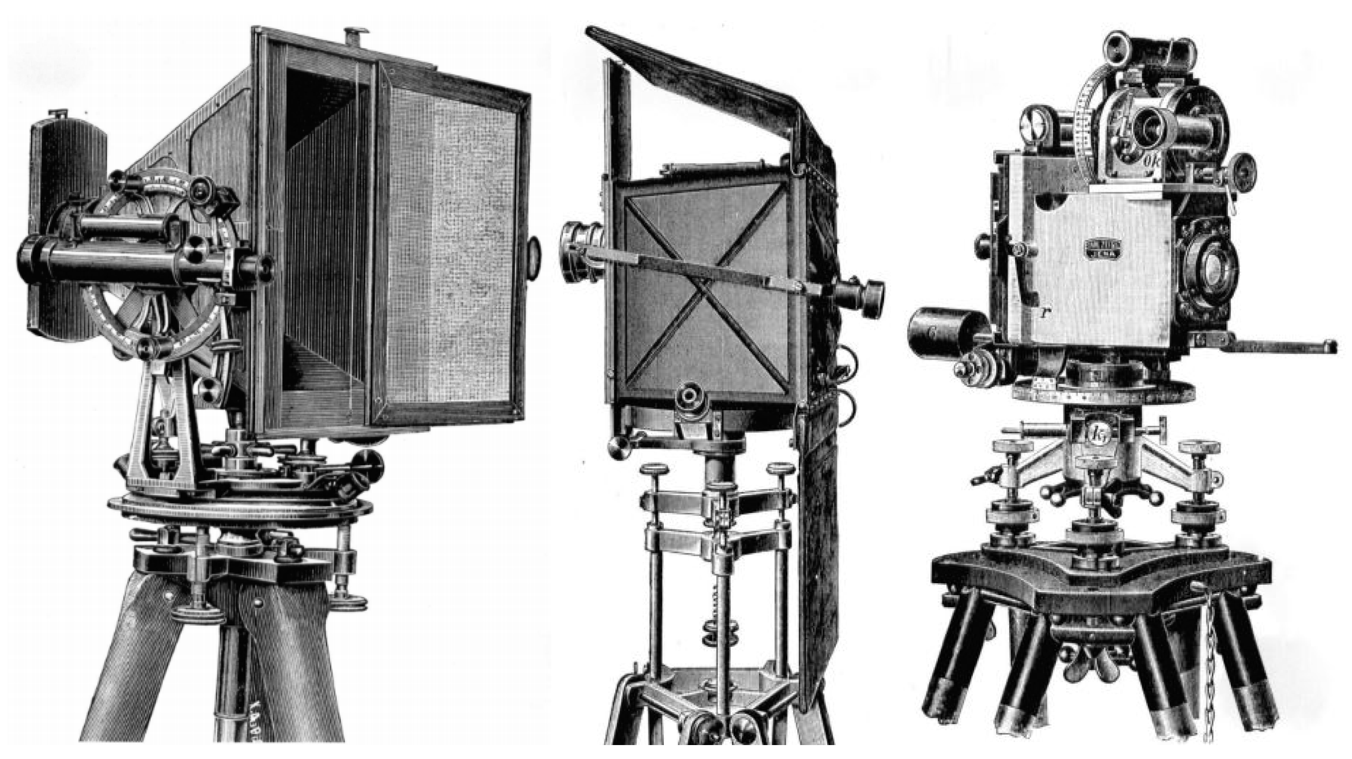
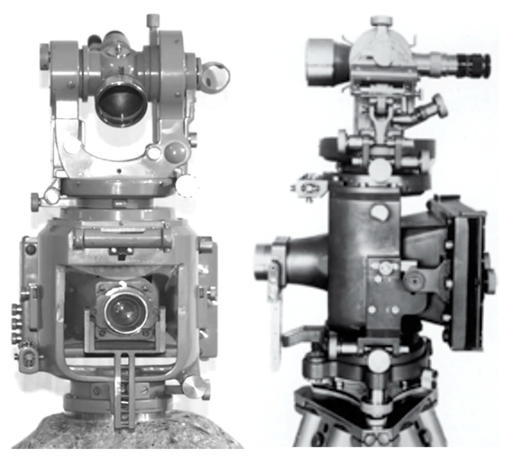
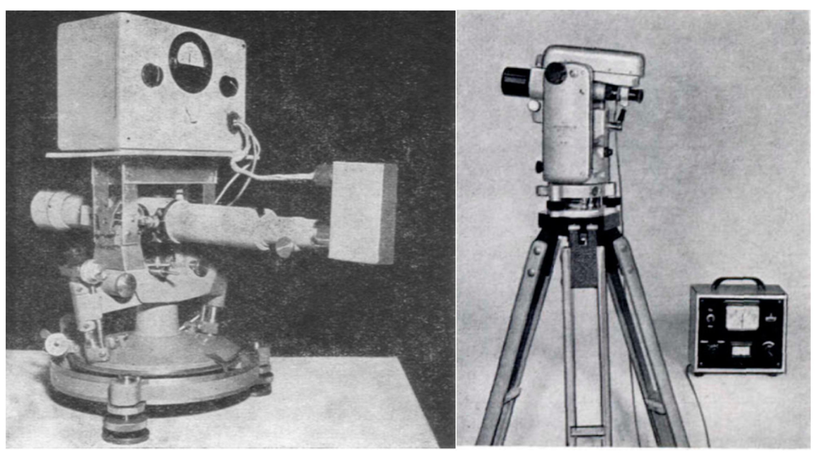
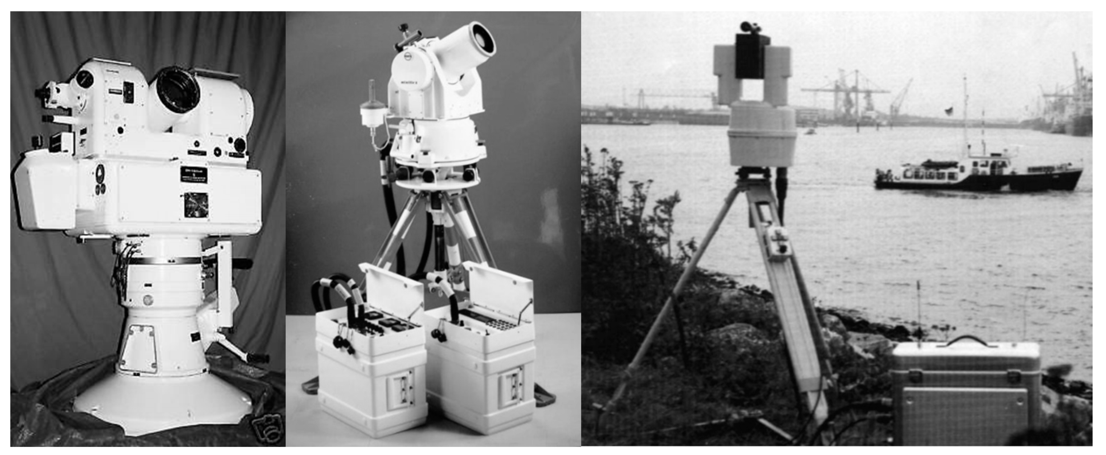
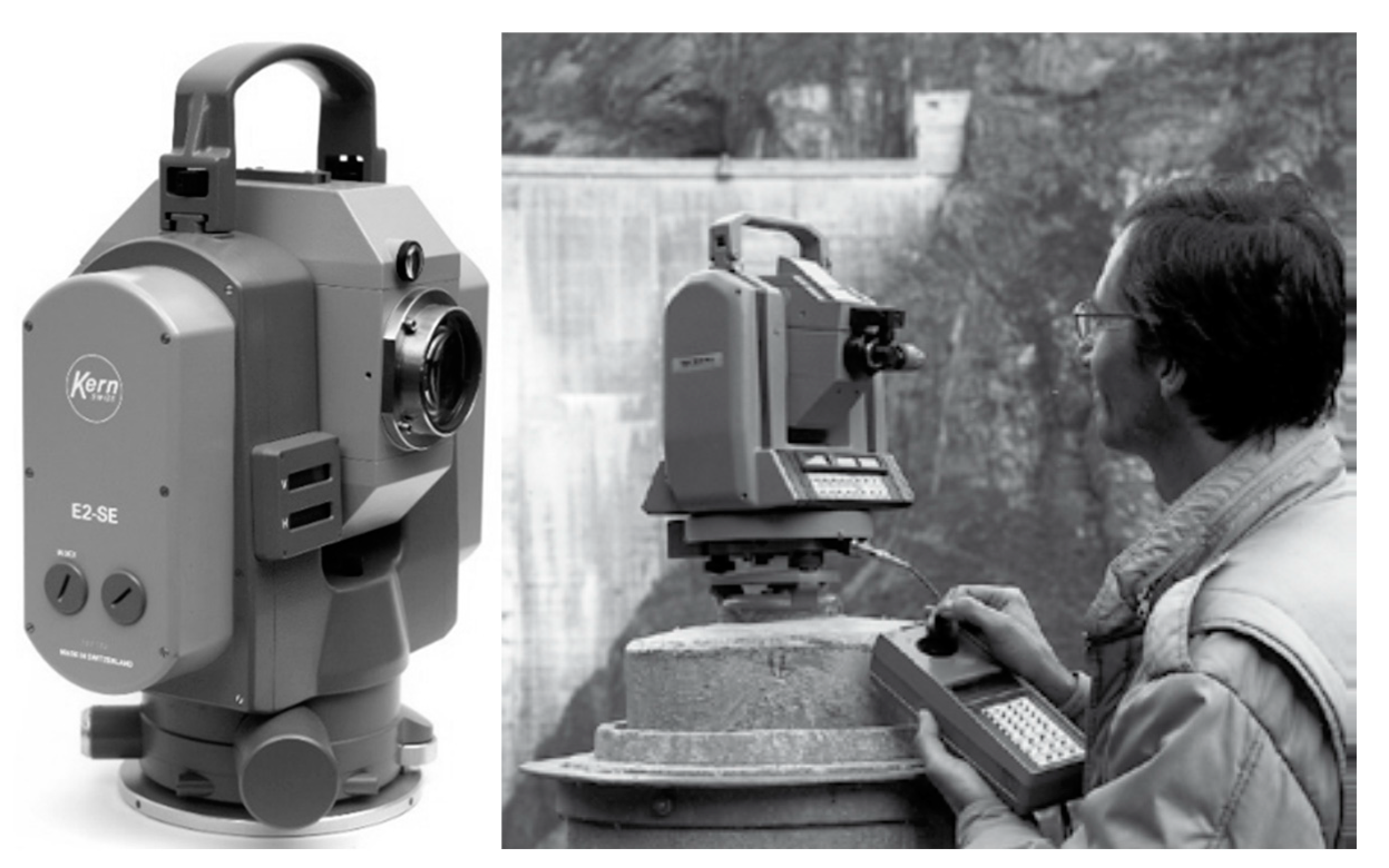
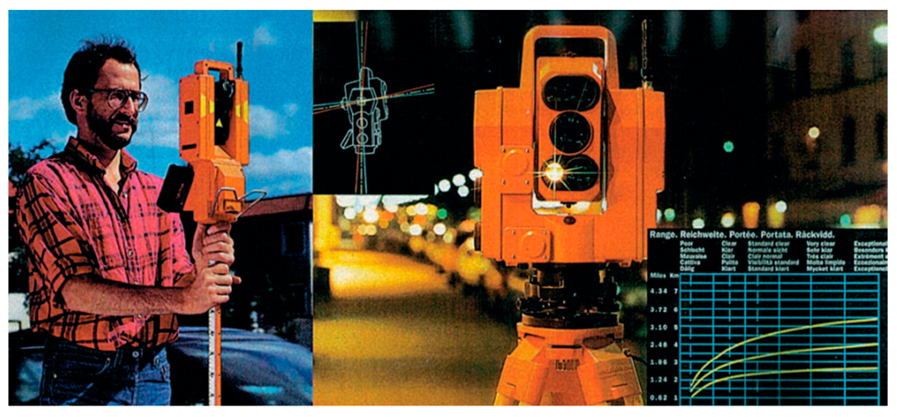
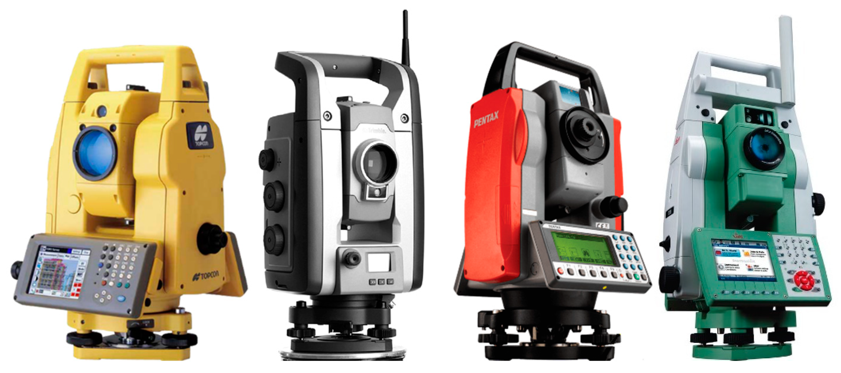
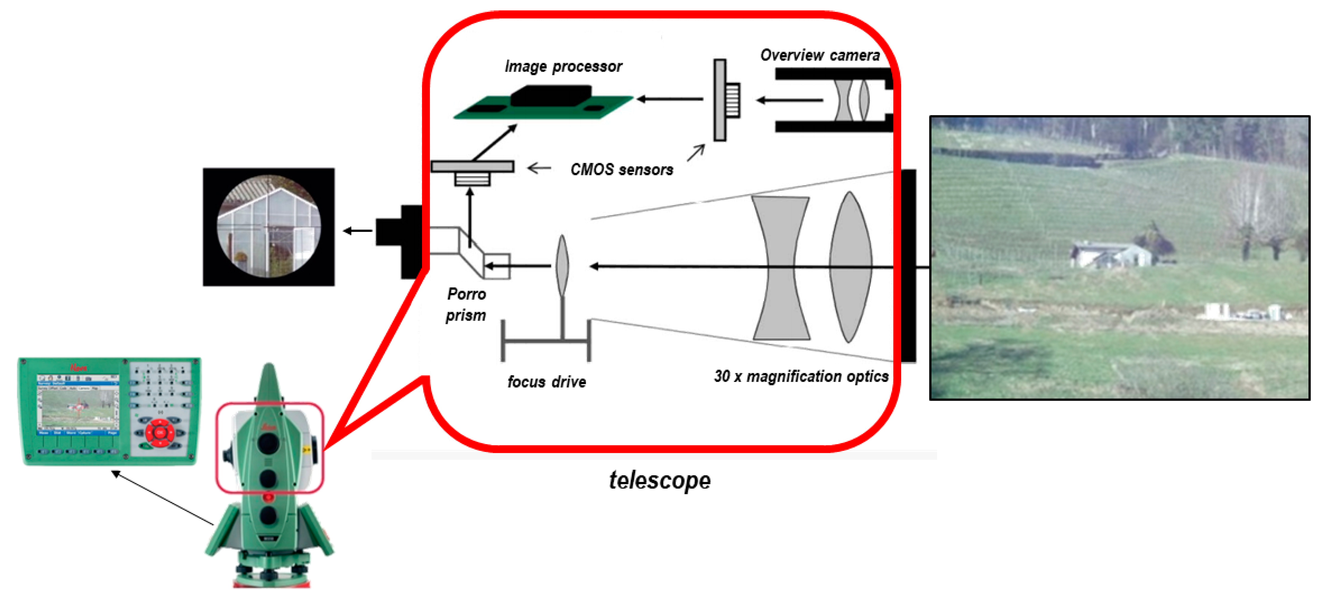
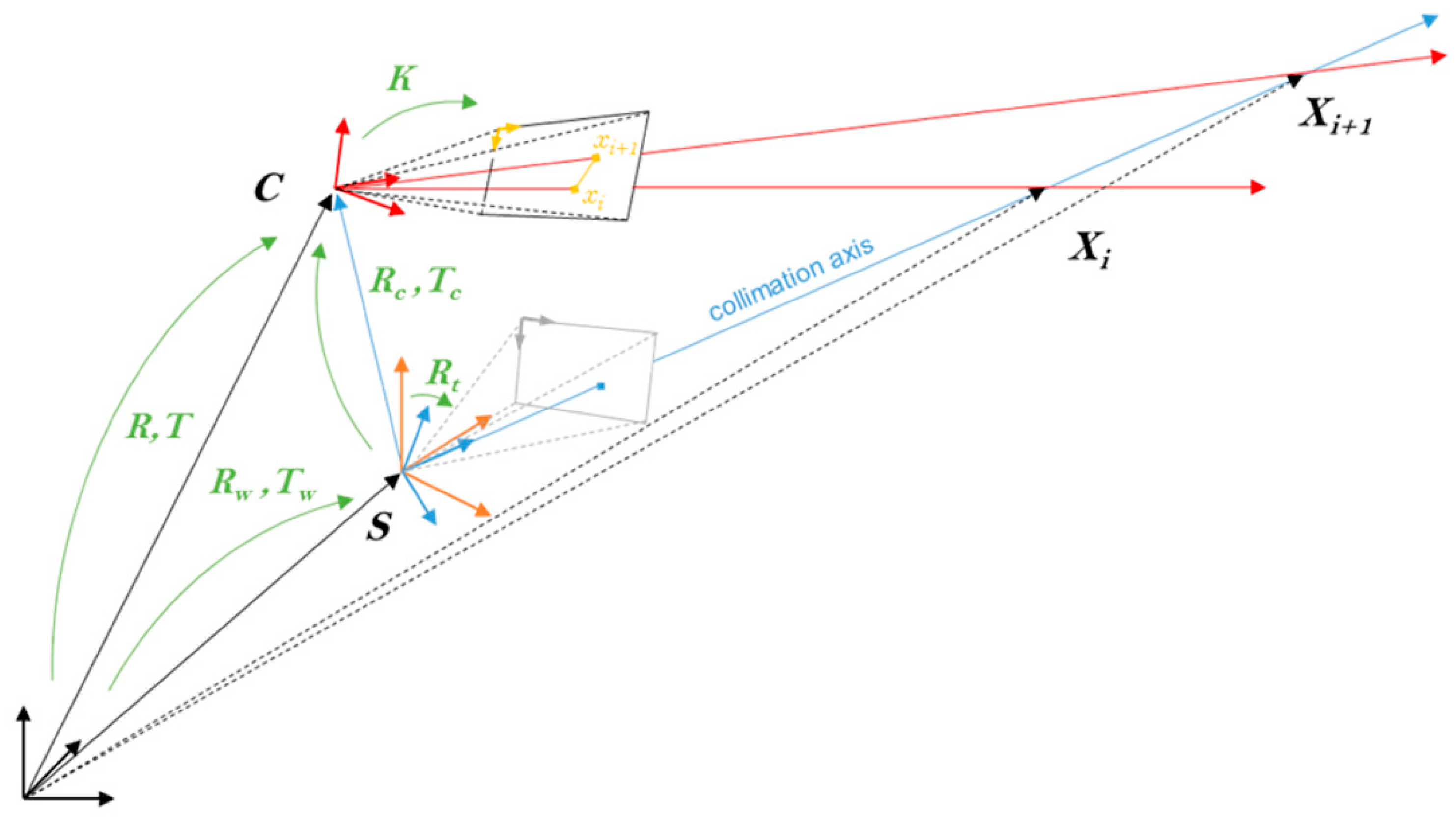
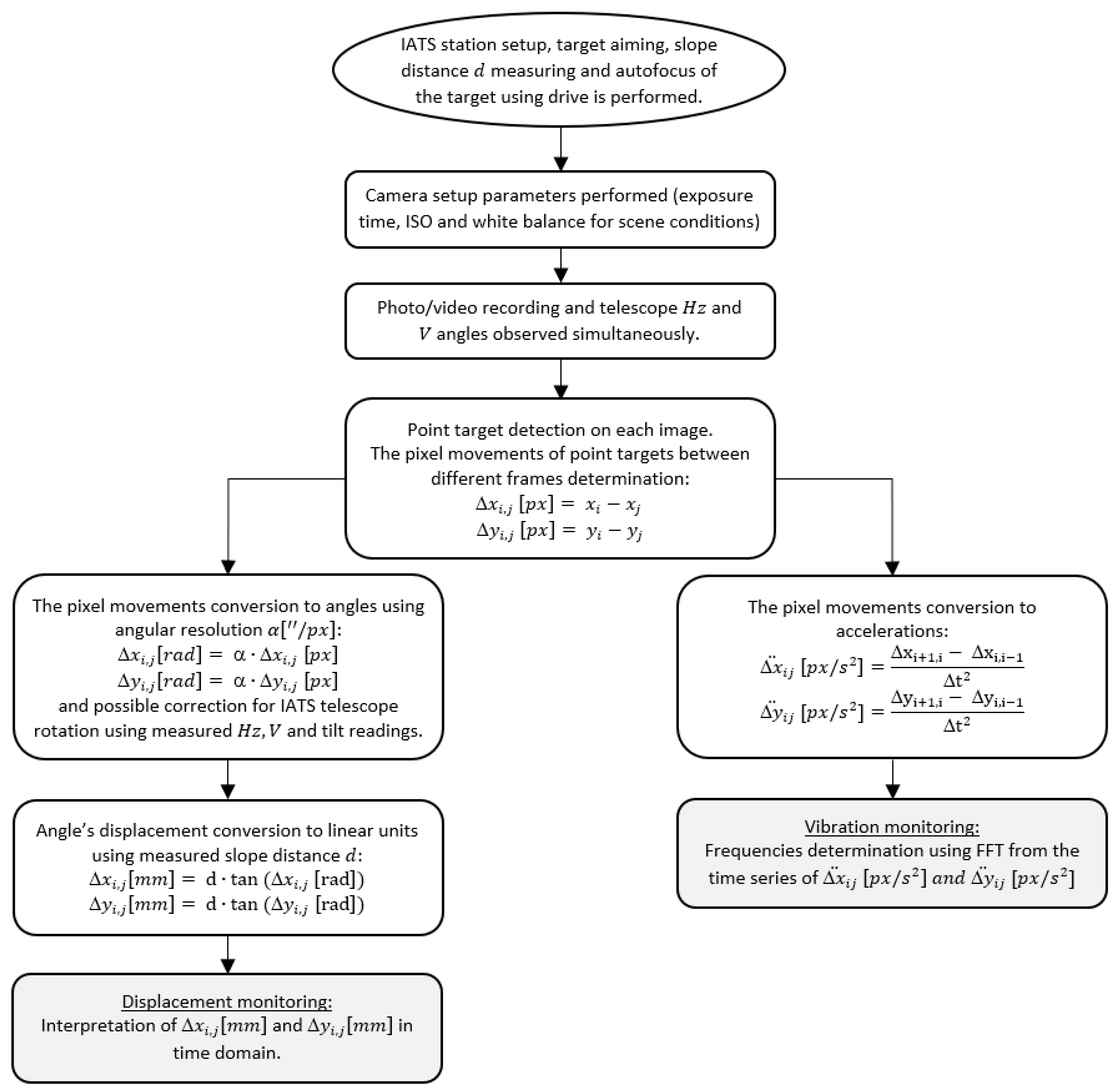
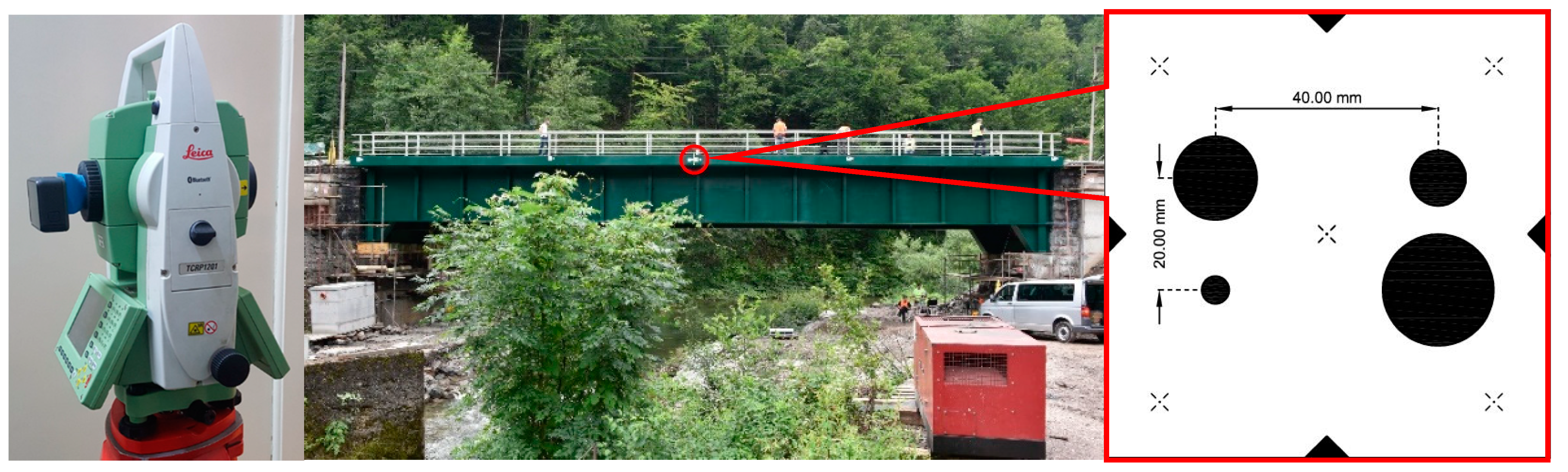
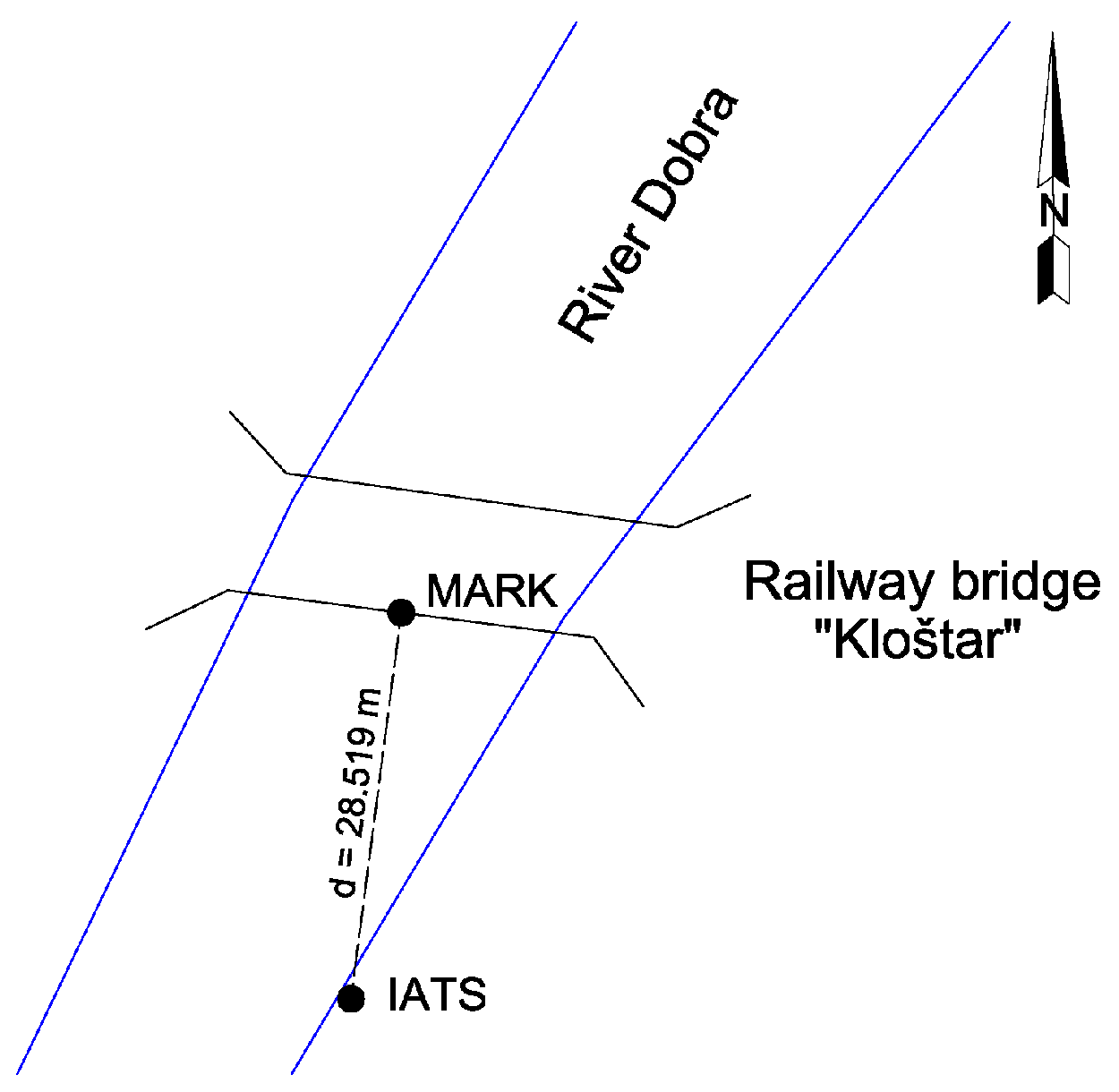
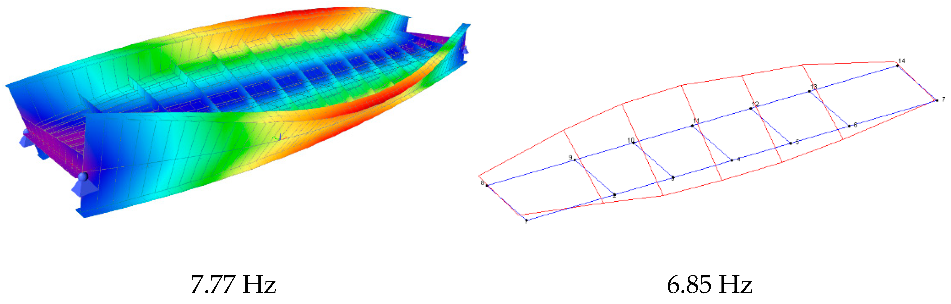
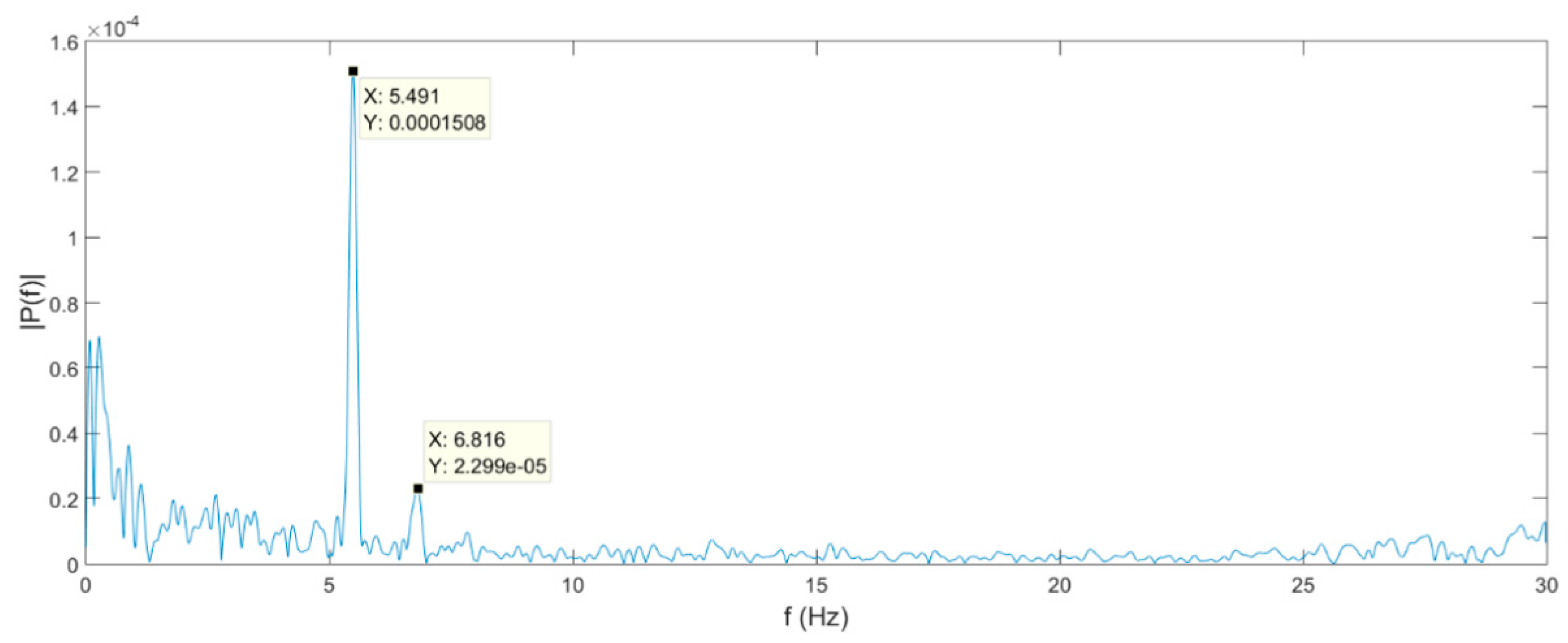
| Specifications | Leica TS60 | Trimble S9 | Topcon DS-200i |
|---|---|---|---|
| Camera/sensor | 2×/CMOS | 1×/CMOS | 1×/CMOS |
| Resolution | 5 MPx | 3 MPx | 5 MPx |
| Fps | 20 Hz | 5 Hz | Live video 1 |
| FOV overview/telescope | 15.5° × 11.7°/1.3° × 1.0° | 16.5° × 12.3°/✗ | Ultra-wide 1/✗ |
| Zoom overview/telescope | 8×/30× | 8×/✗ | 1 |
| Accuracy distance (prism) | 0.6 mm + 1 ppm | 0.8 mm + 1 ppm | 1.5 mm + 2 ppm |
| Accuracy distance (non-prism) | 2 mm + 2 ppm | 2 mm + 2 ppm | 2 mm + 2 ppm |
| Accuracy Hz and V | 0.5″ | 0.5″ | 1″ |
| Scanning function | ✗ | • | ✗ |
| Year released | 2015 | 2015 | 2014 |
1 Specification is not available; ✗—not integrated; •—optional.
| Specifications | Leica MS60 | Trimble SX 12 | Topcon GTL-1000 |
|---|---|---|---|
 |  |  | |
| Camera/sensor | 2×/CMOS | 3×/CMOS | 1×/CMOS |
| Resolution | 5 MPx | 8.1 MPx | 5 MPx |
| Fps | 20 Hz | 15 Hz | Live video |
| FOV overview/telescope | 15.5° × 11.7°/1.3° × 1.0° | 2 Total 360° × 300° | 270° × 360°/✗ |
| Zoom overview/telescope | 8×/30× | 107× 3 | 1 |
| Accuracy distance (prism) | 1 mm + 1.5 ppm | 1 mm + 1.5 ppm | 1 mm + 2 ppm |
| Accuracy distance (non-prism) | 2 mm + 2 ppm | 2 mm + 1.5 ppm | 2 mm + 2 ppm |
| Accuracy Hz and V | 1″ | 1″ | 1″ |
| Scan rate | 30,000 Hz | 26,600 Hz | 100,000 Hz |
| Year released | 2020 | 2021 | 2019 |
1 Specification is not available; 2 FOV using all three cameras; 3 main camera zoom; ✗—not integrated.
Table 3.
Different types of TS according to integrated sensors and functions.
| TS | RTS | IATS | IASTS | |
|---|---|---|---|---|
| EDM | ✓ | ✓ | ✓ | ✓ |
| Reflectorless EDM | • | • | ✓ | ✓ |
| Data registration | ✓ | ✓ | ✓ | ✓ |
| Motorization | ✗ | ✓ | ✓ | ✓ |
| Image sensor | ✗ | ✓/• | ✓ | ✓ |
| Automated aiming | ✗ | ✓/• | ✓ | ✓ |
| Tracking | ✗ | ✓/• | ✓ | ✓ |
| Imaging | ✗ | ✗ | ✓ | ✓ |
| Scanning | ✗ | ✗ | ✗/• | ✓ |
✓—integrated; ✗—not integrated; •—optional.
Publisher’s Note: MDPI stays neutral with regard to jurisdictional claims in published maps and institutional affiliations. |
© 2021 by the authors. Licensee MDPI, Basel, Switzerland. This article is an open access article distributed under the terms and conditions of the Creative Commons Attribution (CC BY) license (https://creativecommons.org/licenses/by/4.0/).
Share and Cite
MDPI and ACS Style
Paar, R.; Roić, M.; Marendić, A.; Miletić, S. Technological Development and Application of Photo and Video Theodolites. Appl. Sci. 2021, 11, 3893. https://doi.org/10.3390/app11093893
AMA Style
Paar R, Roić M, Marendić A, Miletić S. Technological Development and Application of Photo and Video Theodolites. Applied Sciences. 2021; 11(9):3893. https://doi.org/10.3390/app11093893
Chicago/Turabian StylePaar, Rinaldo, Miodrag Roić, Ante Marendić, and Stjepan Miletić. 2021. "Technological Development and Application of Photo and Video Theodolites" Applied Sciences 11, no. 9: 3893. https://doi.org/10.3390/app11093893
Note that from the first issue of 2016, this journal uses article numbers instead of page numbers. See further details here.