
Refrigerant Charge Prediction of Vapor Compression Air Conditioner Based on Start-Up Characteristics

1
Department of Mechanical Engineering, Graduate School, Kookmin University, Jeongnueng-ro 77, Seongbuk-gu, Seoul 02707, Korea
2
School of Mechanical Engineering, Kookmin University, Jeongnueng-ro 77, Seongbuk-gu, Seoul 02707, Korea
*
Author to whom correspondence should be addressed.
Appl. Sci. 2021, 11(4), 1780; https://doi.org/10.3390/app11041780
Submission received: 11 January 2021
/
Revised: 31 January 2021
/
Accepted: 12 February 2021
/
Published: 17 February 2021
(This article belongs to the Special Issue Sciences and Innovations in Heat Pump/Refrigeration: Volume II)
Abstract
:Refrigerant charge faults, which occur frequently, increase the energy loss and may fatally damage the system. Refrigerant leakage is difficult to detect and diagnose until the fault has reached a severe degree. Various techniques have been developed to predict the refrigerant charge amount based on steady-state operation; however, steady-state experiments used to develop prediction models for the refrigerant charge amount are expensive and time-consuming. In this study, a prediction model was established with dynamic experimental data to overcome these deficiencies. The dynamic models for the condensation temperature, degree of subcooling, compressor discharge temperature, and power consumption were developed with a regression support vector machine (r-SVM) model and start-up experimental data. The dynamic models for the condensation temperature and degree of subcooling can predict the distinct start-up characteristics depending on the refrigerant charge amount. Moreover, the estimated root mean square error (RMSE) of the condensation temperature and degree of subcooling of the test data are 0.53 and 0.84 °C, respectively. The refrigerant charge is one of the predictors that defines the dynamic characteristics. The refrigerant charge can be estimated by minimizing the RMSE of the predicted values of the dynamic models and experimental data. When the dynamic characteristics of the two predictor variables, “condensation temperature” and “degree of subcooling” are used together, the average prediction error of the test data is 2.54%. The proposed method, which uses the dynamic model during start-up operation, is an effective technique for predicting the refrigerant charge amount.
1. Introduction
In response to global warming and climate change, governments worldwide have implemented related policies and technical efforts that include the use of renewable energies and the increase in the energy efficiency to reduce energy consumption and greenhouse gas (GHG) emissions.
In the United States in 2015, approximately 40% of the total consumed energy was used in commercial and residential buildings [1]. Approximately 41% of the energy consumed in the building sector was used for heating and cooling, and between 15% and 30% was wasted owing to poor maintenance or inadequate control [2]. To operate and maintain air conditioning systems efficiently, the energy efficiency should be maximized through optimal control and with fault diagnosis technology.
Faults in air conditioning systems can be classified into hard and soft faults. Hard faults that lead to system halt can be easily detected and diagnosed. By contrast, soft faults such as refrigerant leakage and heat exchanger fouling are difficult to detect and diagnose before the faults reaches a severe degree; this can lead to energy loss and a damaged system. Refrigerant charge fault is the next most costly fault among the different types of heat pump faults, except for electrical fault; the former are mainly caused by refrigerant leakage [3].
The refrigerant charge amount is one of the main parameters that affect the performance and energy consumption of heat pumps [4,5,6,7]. When the refrigerant charge exceeds 90% of the rated charge, the effect on the COP and cooling capacity is small. The refrigeration capacity and COP decrease if the initial charge of the system is low or if the charge decreases owing to leakage during operation. Even under an overcharge, the COP decreases owing to the increasing compression work; however, the performance of the air conditioner is more severely degraded under undercharging than under overcharging [8]. Refrigerant charge faults occur frequently owing to refrigerant leakage, equipment relocation, the installation of piping systems, and incorrect initial charging. Direct emission and performance degradation by refrigerant leakage will have an impact on global warming [9]. Accordingly, many research studies have been conducted to detect refrigerant charge faults [10,11,12,13,14,15,16].
Several researchers have predicted the refrigerant charge amount by monitoring air conditioning systems in real time [14,15,16]. For instance, Grace et al. implemented a relatively inexpensive leak detection system with the degree of superheat and subcooling as detection parameters [14]. In addition, G. Li and H. Li tried to monitor continuously the refrigerant charge level by constructing a monitoring system with a virtual refrigerant charge sensor [14,15,16]. Since variable speed compressors are commonly adopted in high-efficiency air conditioners, researchers have studied the dynamic characteristics and modeling of refrigeration cycles for the stable control of systems equipped with variable speed compressors [17,18,19,20,21]. Accordingly, research studies of the detection of the refrigerant charge amount have been extended to VRF (Variable Refrigerant Flow) systems with complex physical structures such as variable speed compressors, electric expansion valve (EEVs), and heat recovery devices [14,18,19,20,21,22]. Liu et al. proposed a relatively simple model that can be developed in a short time with a statistical method belonging to the category of history-based method [22].
These studies have been based on steady-state operating data. To develop a model for the prediction of the refrigerant charge amount, experimental data that reflect the characteristics of a system under steady-state conditions are required; the related experiments, which are conducted to increase the prediction performance of the model, are expensive and time-consuming. In addition, because the actual operation continuously fluctuates according to the changes in the outdoor temperature and cooling load, the extraction of steady-state data for predicting the refrigerant charge amount requires a long operation period, which may reduce the accuracy of the predictions.
In this paper, a prediction model based on dynamic experimental data for overcoming these deficiencies is proposed. Dynamic experimental data for the model development are easy and fast to obtain; thus, the acquisition time is reduced. In the study of the dynamic characteristics of refrigeration systems, physical and data-based models are applied [14,15,16,17]. Moreover, more and more researchers study dynamic models with machine learning owing to the improved computational speed [23,24,25,26,27,28,29,30]. In this study, the dynamic behavior of a refrigeration system was modeled with a regression support vector machine (r-SVM, which is a data-based model). The model was used to confirm that the initial dynamic characteristics of the refrigeration system vary according to the refrigerant charge amount, which enables the prediction of the latter.
2. Experiment
2.1. Experimental Setup
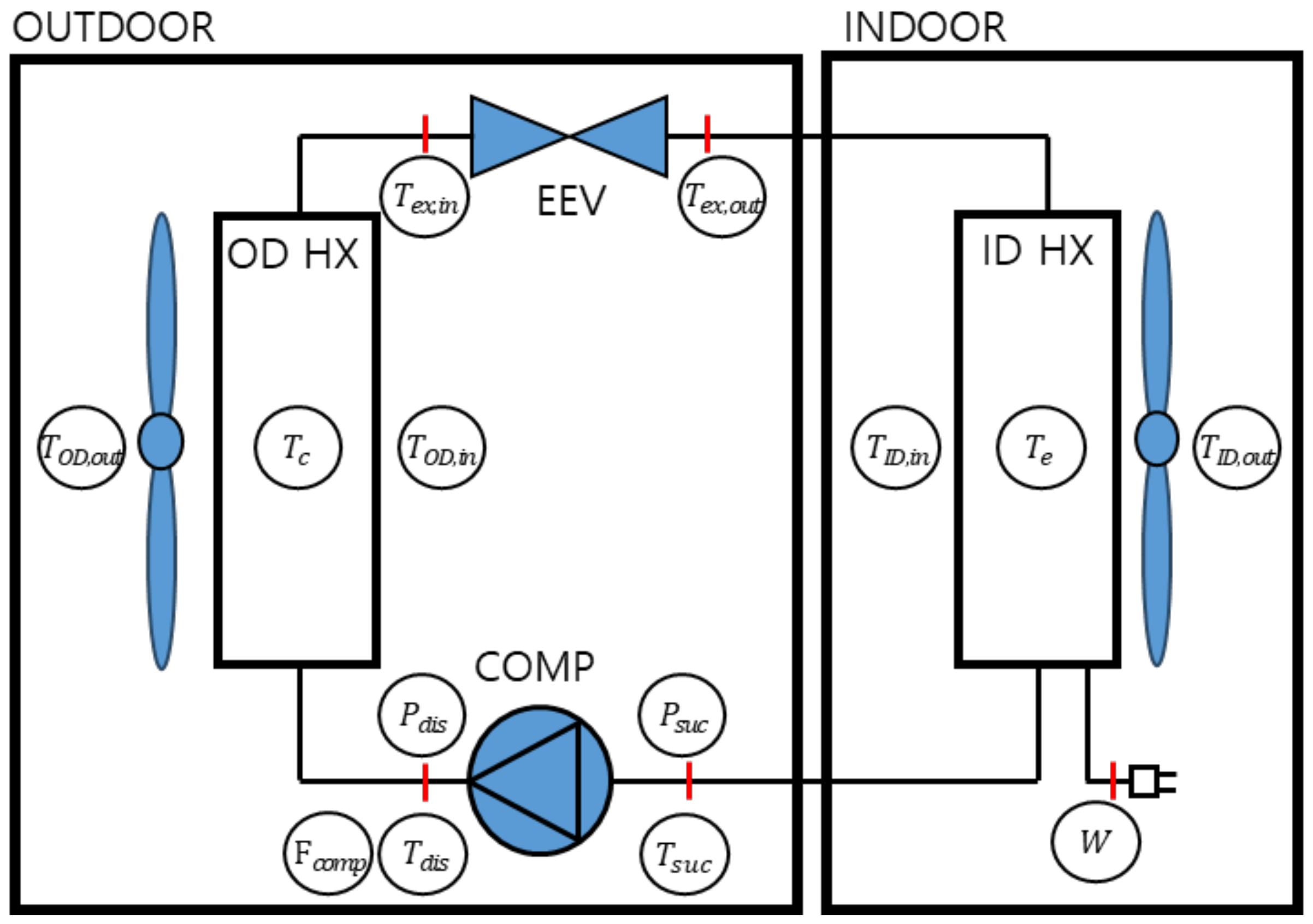
To present the start-up characteristics of an air conditioner, Figure 1 shows a schematic diagram of the experimental apparatus. The split-type air conditioner with a rated cooling capacity of 3.6 kW consists of a variable speed compressor, an electronic expansion valve, an evaporator, and a condenser. The indoor and outdoor units of the air conditioner are installed in a thermal chamber with two rooms that can simulate indoor and outdoor temperature and humidity conditions. The air and refrigerant temperatures at the inlet and outlet of the main components of the system were measured with T-type thermocouples (uncertainty: 0.5 °C, range: −250 to 350 °C); the refrigerant temperature was measured by a thermocouple attached to the outer wall surface of the tube. In addition, the compressor suction and discharge pressures were measured with pressure transducers (uncertainty: 0.25%, range: 0 to 3500 kPa) at the inlet and outlet of the compressor. The power consumption was measured with a power meter (accuracy: 0.5% of reading, range: 0 to 3 kW), the frequency of compressor input power was obtained by FFT (Fast Fourier Transform) of the measured voltage of power.
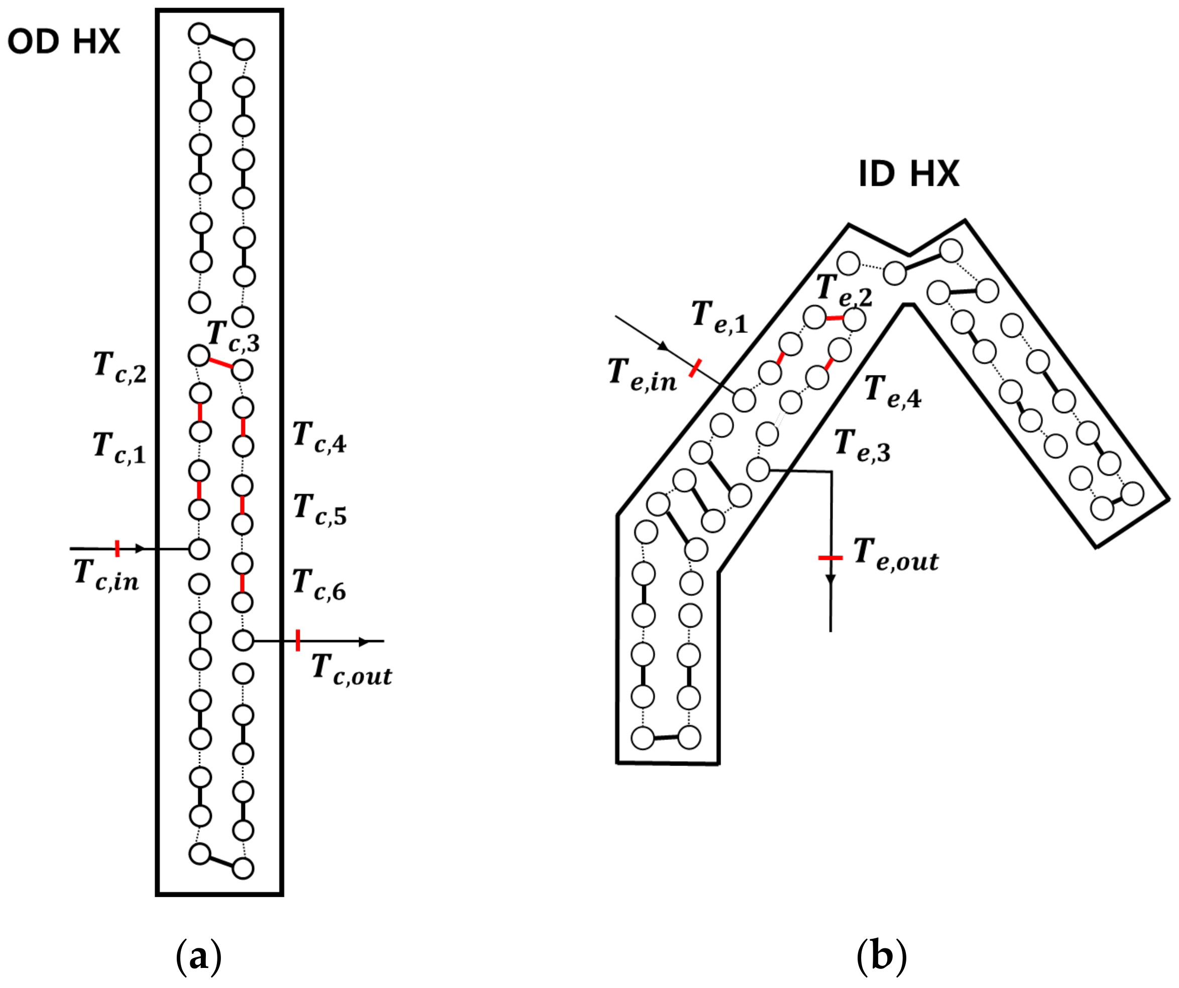
The thermocouples were installed at the points in Figure 2 to investigate the state changes of the refrigerant in the condenser and evaporator during initial operation. The condenser has eight temperature measurement points (in numerical order) between the inlet and outlet in one circuit, and the evaporator has six thermocouples between the inlet and outlet. The measurement values were recorded at intervals of 1 s and stored with a data logger. The 20 measured variables are listed in Table 1.
2.2. Experimental Method and Condition
The experiment was conducted 47 times; 35 of the data were used as training data, and 12 were used as test data. The experiment started when the initial indoor and outdoor temperatures reached the conditions in Table 2. The maximum deviation of outdoor temperature in the chamber was ±0.5 °C during each test. When the air conditioner started to run, the indoor temperature began to decrease. Each experiment was conducted for 600 s, and the experimental data were measured for 600 s at 1 s intervals. After each experiment, the equipment was suspended for 2 h to achieve uniform initial conditions.
The refrigerant used in the experiment was R-410A, and the rated charge amount was 850 g. The air conditioner was charged from 550 to 950 g for training data and 600 to 900 g for test data, with charge steps of 100 g. Refrigerant charge was carried out subsequently, being the measuring error of the balance of 0.05% of reading. Charge uncertainty is estimated as shown in Table 2.
3. Start-Up Characteristics
3.1. Start-Up Characteristics with Rated Refrigerant Charge
The dynamic characteristics during the start-up and shutdown of the air conditioner can be described based on the refrigerant movement inside the system [18]. When the compressor starts, the refrigerant is drawn from the evaporator and suction line and discharged into the condenser by the compressor. In the early stage of the compressor operation, the amount of refrigerant that condenses in the condenser is insufficient, and the refrigerant exits the condenser with the gas mixture; thus, the refrigerant entering the evaporator is insufficient for replacing the refrigerant that has been sucked out of the evaporator by the compressor. Consequently, the mass of the refrigerant in the evaporator decreases continuously, and the pressure and temperature change rapidly. The compressor continuously draws the refrigerant from the evaporator outlet and discharges it into the condenser; thus, the mass of the refrigerant in the condenser increases, and the refrigerant vapor gradually condenses. As the refrigerant at the outlet of the condenser becomes subcooled, the fluctuations of the pressure and temperature slow down.
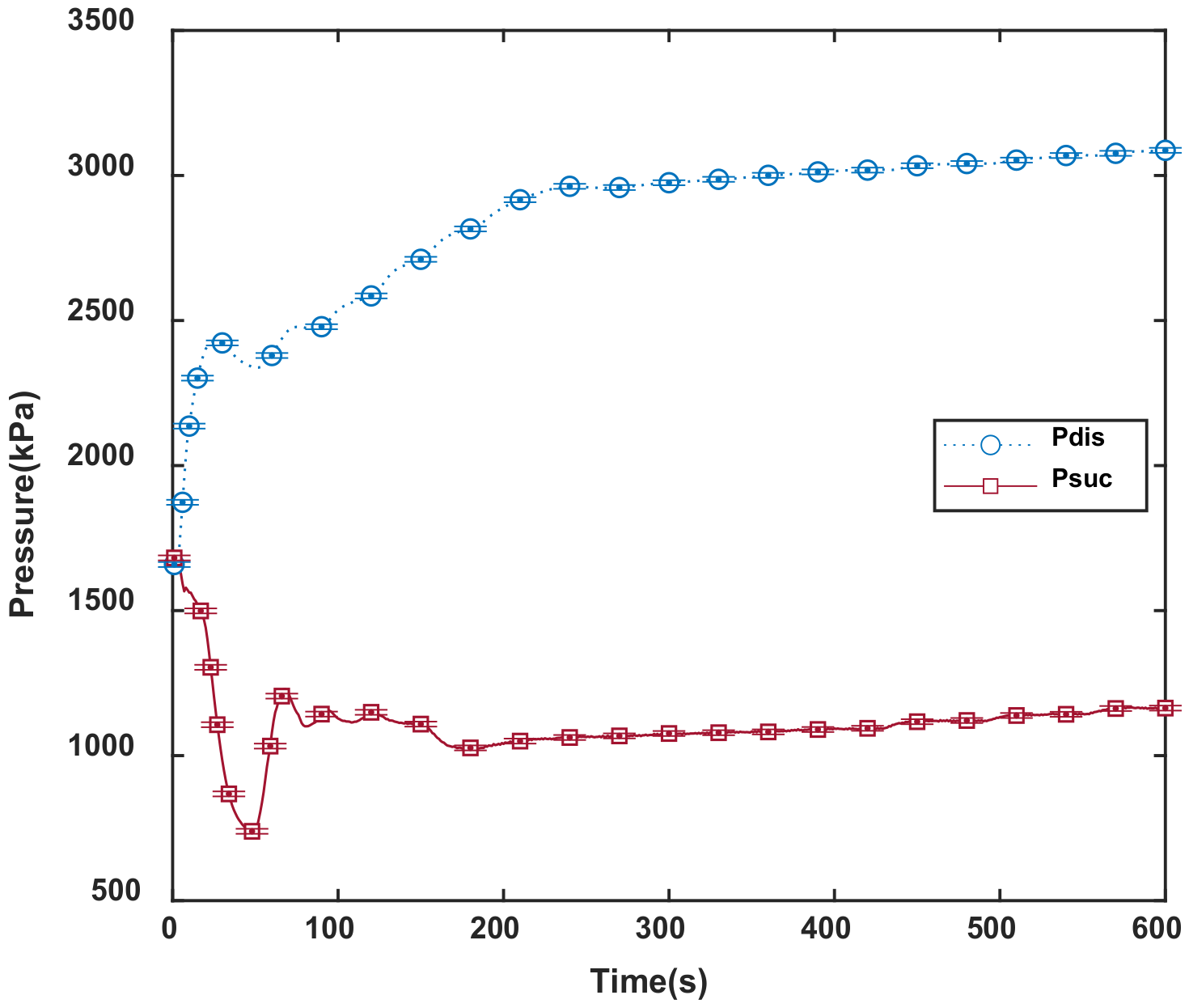
The results in this study are very similar to those of the study described above [18]. Figure 3 and Figure 4 present the dynamic characteristics of the main components of the system at a rated refrigerant charge and outdoor and initial indoor temperatures of 35 °C. Figure 3 shows the change in the discharge and suction pressures of the compressor according to the elapsed time during the initial operation of the air conditioner. The discharge pressure rapidly increased until 70 s owing to the operation of the compressor; subsequently, its slope decreased, and the discharge pressure converged to the steady-state value. The suction pressure greatly decreased in the first 80 s and then increased again until 100 s. Afterward, the pressure increased gradually and tended to converge to a steady-state value.
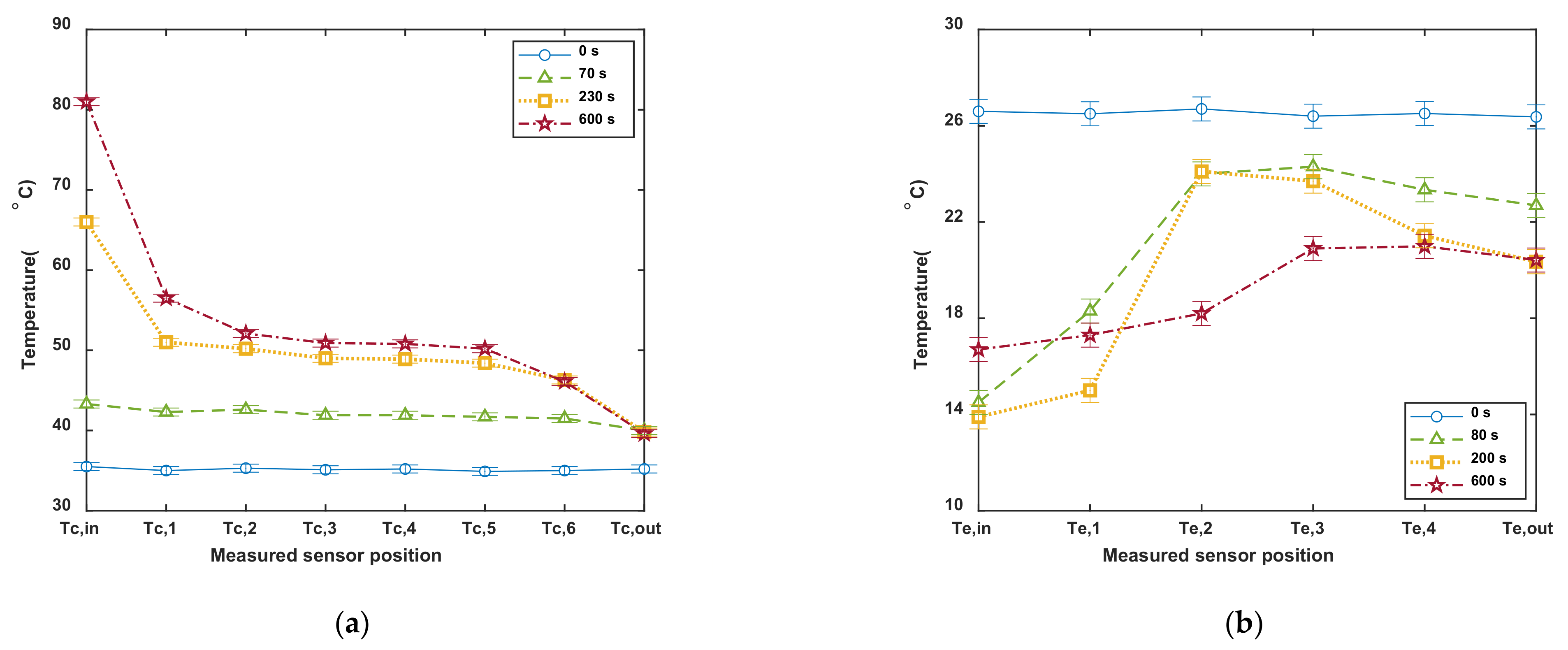
The temperature distributions in the flow direction of the refrigerant in the condenser and evaporator at several time points after the start-up are shown in Figure 4. Before operation, the internal temperature of the condenser was uniform; it can be inferred that most of the condenser was occupied by superheated vapor. As the compressor started to run, the overall temperature of the condenser increased, and the refrigerant condensed and became subcooled at the outlet. After 230 s, three distinct phases appeared in the condenser; the occurrence of superheated refrigerant at the inlet and subcooled refrigerant at the exit can be clearly confirmed.
In addition, the temperature of the evaporator was uniform before the operation of the air conditioner. As shown in Figure 3, the evaporation pressure decreased sharply owing to the operation of the compressor; thus, the temperature of the refrigerant at the inlet of the evaporator decreased at first. Subsequently, the superheating point shifted to the exit, and the saturated refrigerant section gradually increased. The evaporation temperature decreased rapidly at the beginning and then gradually increased over time.
3.2. Start-Up Characteristics with Refrigerant Charge
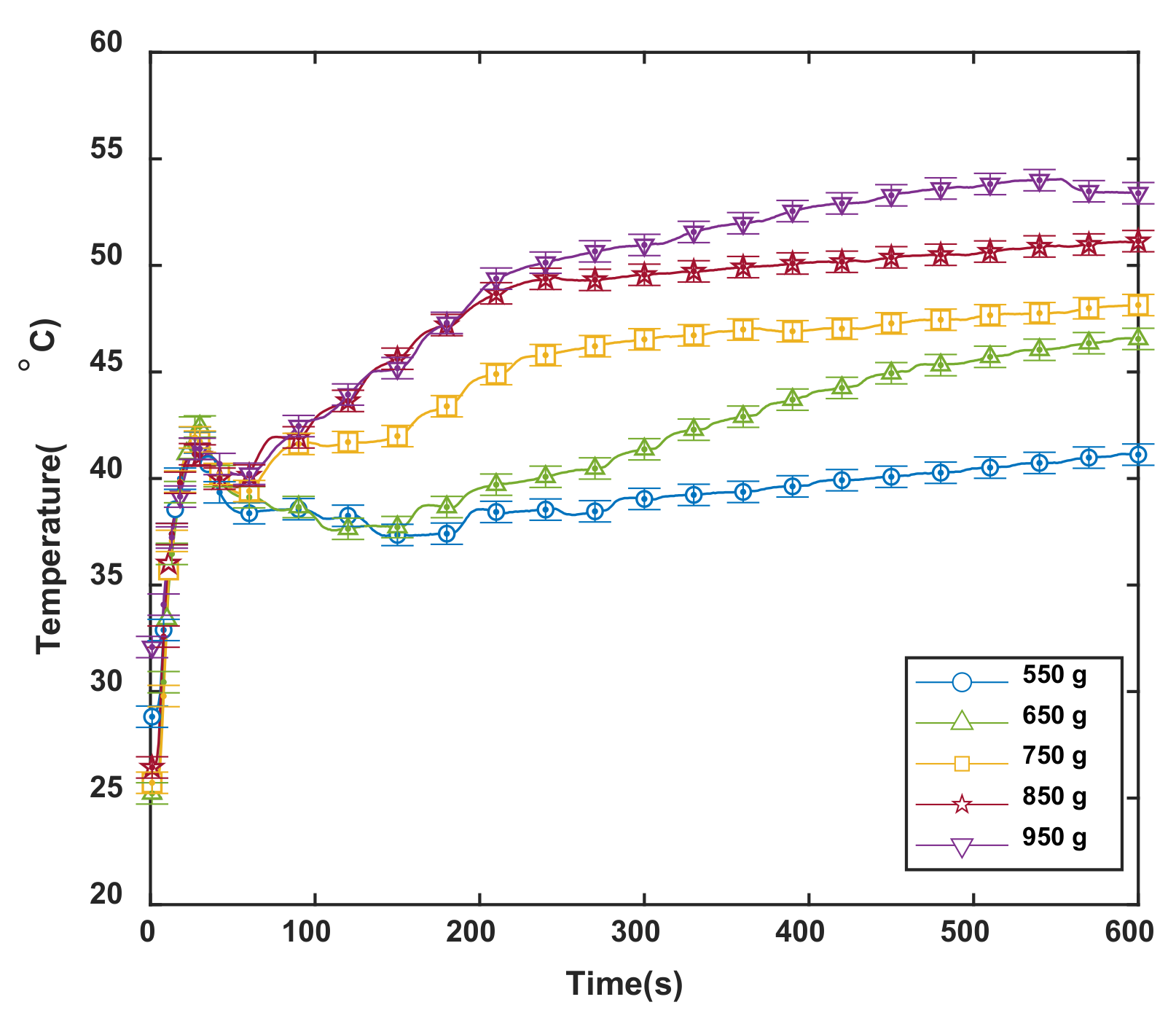
The start-up characteristics were investigated according to the refrigerant charge at outdoor and indoor temperatures of 35 °C. Figure 5 presents the change in the condensation temperature for five refrigerant charges at the beginning of operation. The condensation temperature increased rapidly when the compressor started operating. After approximately 120 s, the condensation temperature varied depending on the refrigerant charge amount; in addition, the condensation temperature increased more rapidly with the increasing refrigerant charge amount. Under overcharging conditions, the dynamic characteristics were similar to the rated charge amount until 220 s and then showed small deviations. After 220 s, the condensation temperature approached the steady-state values for 850 and 750 g; in the 950 and 650 g cases, it increased until approximately 580 s, and that of 550 g kept increasing within the investigated time range (Figure 5).
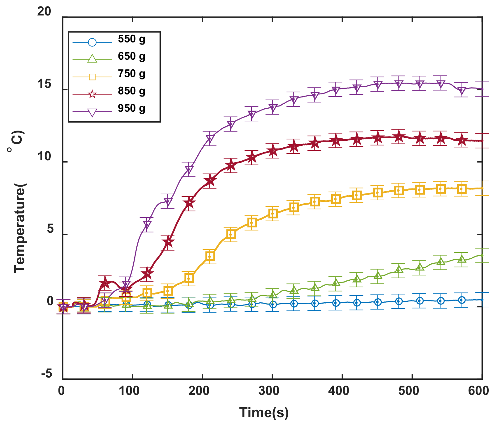
The degree of superheat remained approximately constant, although the refrigerant charge changed owing to the active control of the EEV opening. However, as the refrigerant charge increased owing to the accumulation of refrigerant on the condenser, the condensation pressure increased, which increased the degree of subcooling. Since the degree of subcooling is sensitive to the refrigerant charge amount, it is widely used as a diagnostic parameter to determine the refrigerant charge amount [15,16,17]. As shown in Figure 6, the degree of subcooling exhibited a large increase with increasing refrigerant charge amount after 120 s and slowly decreased after 600 s. The degree of subcooling was proportional to the refrigerant charge amount; in addition, the degree of subcooling of 550 g was zero, which indicates that subcooling did not occur in this case.
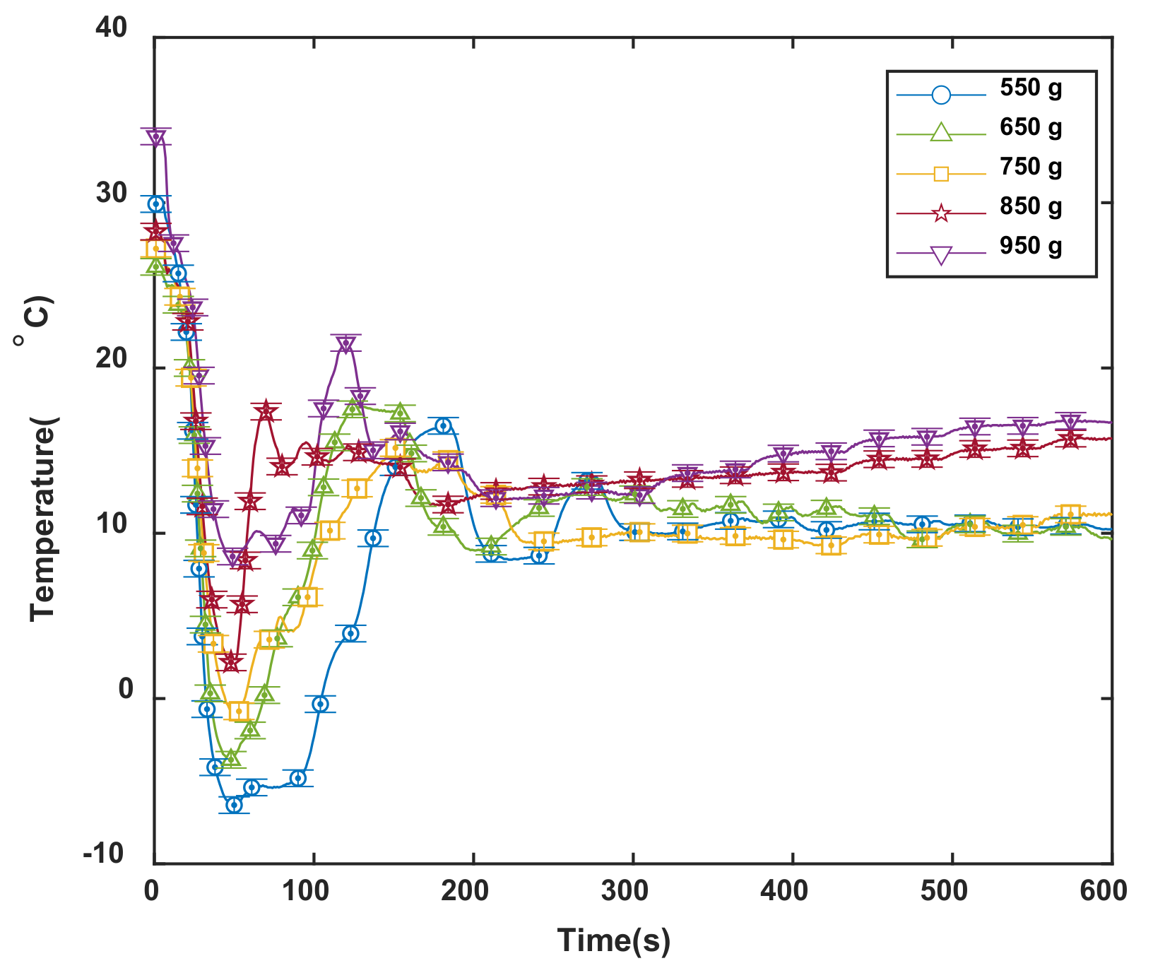
As shown in Figure 7, the evaporation temperature rapidly decreased during the initial 60 s of operation. The lower the refrigerant charge, the less refrigerant was in the evaporator, and the more the evaporation temperature decreased. The evaporation temperature decreased at approximately 30 s until it reached the minimum; afterward, it experienced repeated rebounds until 220 s and stabilized. However, distinguishing the differences in the evaporation temperatures with respect to the refrigerant charge amount was difficult.
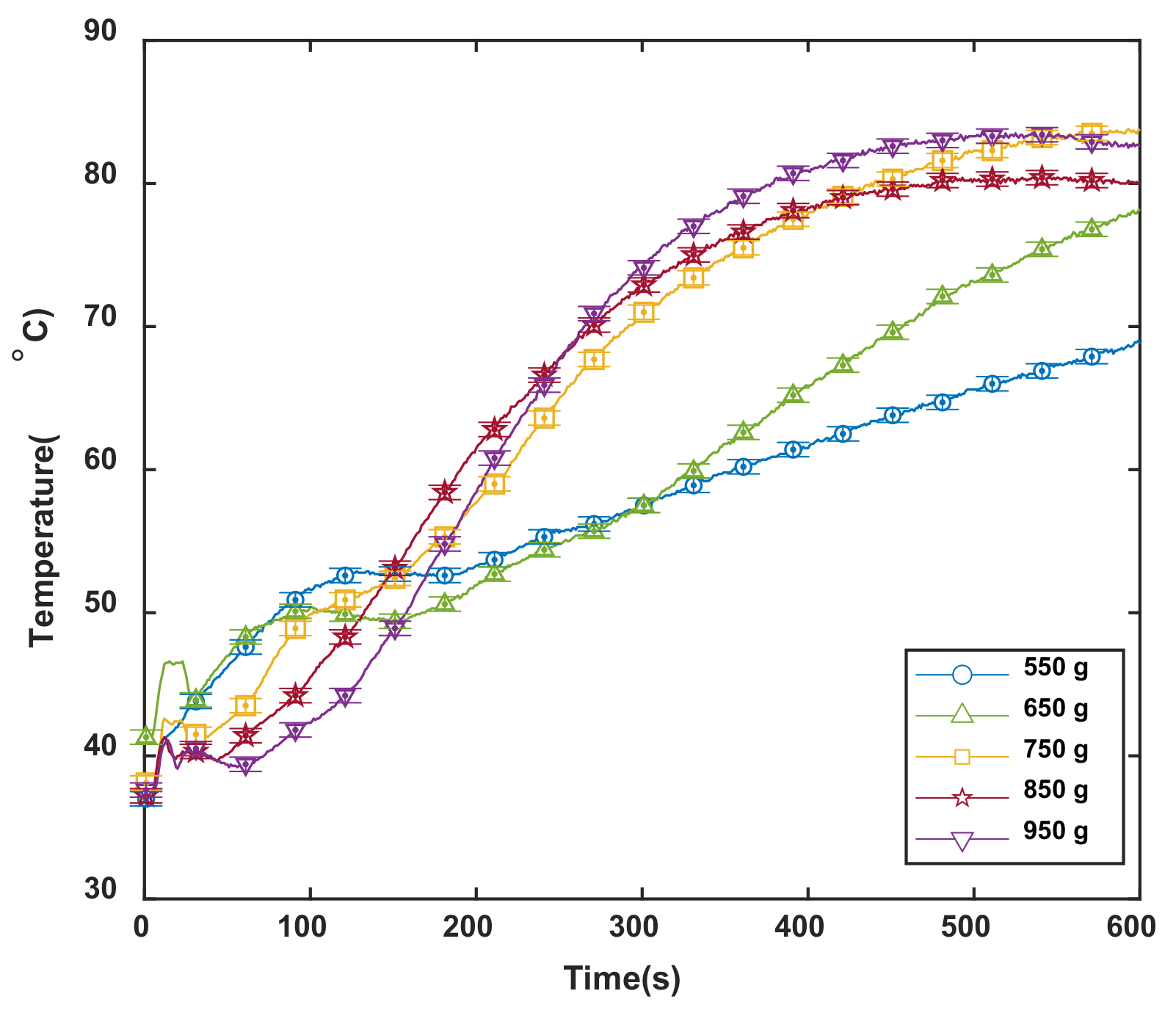
The compressor discharge temperature was affected by the compressor inlet and outlet pressures, which tended to increase as the condensation temperature increased and the evaporation temperature decreased. As shown in Figure 8, the discharge temperature of the compressor increased more rapidly with the decreasing refrigerant charge amount at the beginning of operation because the suction pressure was relatively low at the beginning. After 120 s, the smaller the refrigerant charge, the more moderate the discharge temperature increase because the condensation temperature or pressure was relatively low. The condensation and evaporation temperatures increased with increasing refrigerant charge according to Figure 5 and Figure 7. These two temperature effects on the discharge temperature offset each other; the cases with charge levels of 750 g or higher exhibited similar dynamic characteristics.
4. Model for Prediction of Dynamic Characteristics
The r-SVM model is a regression analysis model that extends the SVM theory; it has been considered an effective prediction method [14,31,32,33,34]. The existing neural network follows the empirical risk minimization (ERM) principle, whereas the SVM model follows the structural risk minimization (SRM) principle. The ERM principle minimizes errors in training data, whereas the SRM principle maintains a balance between the training data and test data errors. Therefore, the SVM principle has a better generalization performance in prediction problems [35].
In this study, a dynamic model was developed based on the r-SVM machine learning model. When the experimental data are {(x1, y1), …, (xm, ym)}, x consists of a multivariate set of predictors with the response variable y. The r-SVM model has the maximal deviation ϵ from the response variable y and tries to find the function f(x) as flat as if possible. In the SVM principle, which is a nonparametric model, f(x) is defined as in Equation (1); < w,x > is the dot product of w and x similar to Equation (2). w is the flatness, and b is the bias. To allow an error higher than ϵ, f(x) can be obtained by introducing the slack variable ξi, ξi* and the penalty constant C, thereby transforming it into a convex optimization problem, as shown in Equation (3):
f(x) = < w,x > + b,
The variables and ranges for the training data were selected by analyzing the dynamic characteristics of the system according to the refrigerant charge amount (Section 3). The dynamic models for the condensation temperature, degree of subcooling, compressor discharge temperature, and power consumption were developed as response variables y with the experimental data measured between 120 and 600 s at intervals of 1 s after the compressor had been operated. As predictors, the variables x defining dynamic models, refrigerant charge amount, compressor input frequency, and indoor and outdoor air inlet temperature were basically selected, and the first time derivatives of the input frequency of the compressor and target model parameter were added considering the transient characteristics of the experimental data (Table 3).
The model was optimized by searching for determining the hyper-parameters C and ϵ that minimize the root mean square error (RMSE) with a grid search method and a K-fold cross-validation method. The RMSE is defined as in Equation (4); ypred and ymeas are the predicted and measured values, respectively. The grid search method determines the optimal parameter by trying discrete values with appropriate intervals within a specified range [36]. The K-fold cross-validation method evaluates a model by dividing the data into K datasets, training the K-1 datasets as training data, and measuring the degree of error with one prediction data piece [37]. Moreover, C (C > 0) is the penalty constant, which determines the trade-off between the flatness of f(x) (decision boundary) and the tolerance for error. The model searches for C and ϵ in the log-scale ranges [0.001 1000] and [0.001 1000] × iqr(y)/13.49, respectively; iqr(y)/13.49 represents an estimate of a tenth of the standard deviation for the interquartile range of the response variable y [38]. The parameter optimization results of the dynamic model for the predictor variables are summarized in Table 4.
In the training phase, the average RMSEs of the prediction models for the condensation temperature and degree of subcooling were 0.51 and 0.83 °C, and the respective average RMSEs of the test data were 0.53 and 0.84 °C, respectively. The trained models for the prediction of the condensation temperature and degree of subcooling effectively predicted new untrained data. However, the compressor discharge temperature had a relatively large error, and the model prediction accuracy decreased owing to the increasing prediction error. The accuracies of the power consumption prediction model for the training and test data were 5.54% and 5.6%, respectively.
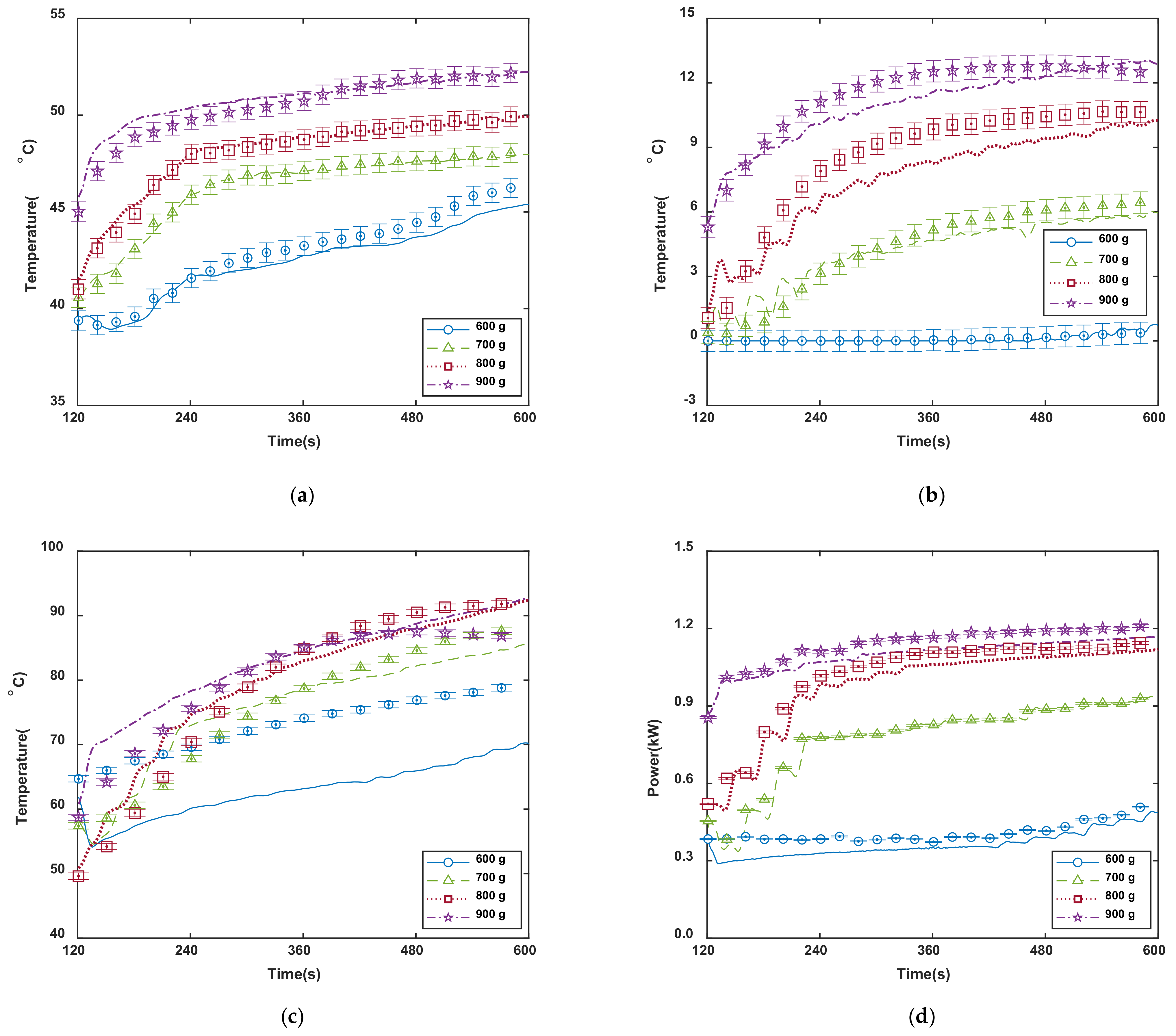
The prediction results of the dynamic models of the condensation temperature, degree of subcooling, compressor discharge temperature, and power consumption developed in this study are compared with the test data in Figure 9. The results correspond to outdoor and initial indoor temperatures of 35 °C and 600, 700, 800, and 900 g refrigerant charge amounts; the curves represent the predicted values of the developed model, while the symbols represent the experimental test data.
The predicted condensation temperature was lower than the experimental result under undercharged conditions and higher under overcharged conditions. The predicted degree of subcooling was lower for all refrigerant charge amounts. These prediction characteristics can be exploited in the prediction of the refrigerant charge amount.
The predicted result of the compressor discharge temperature was poor under undercharged conditions. Moreover, the predicted power consumption tended to be lower than the actual experimental result; nevertheless, the predictions were relatively good and had small errors.
5. Detection of Refrigerant Charge Amount
Detection Results of Refrigerant Charge Amount
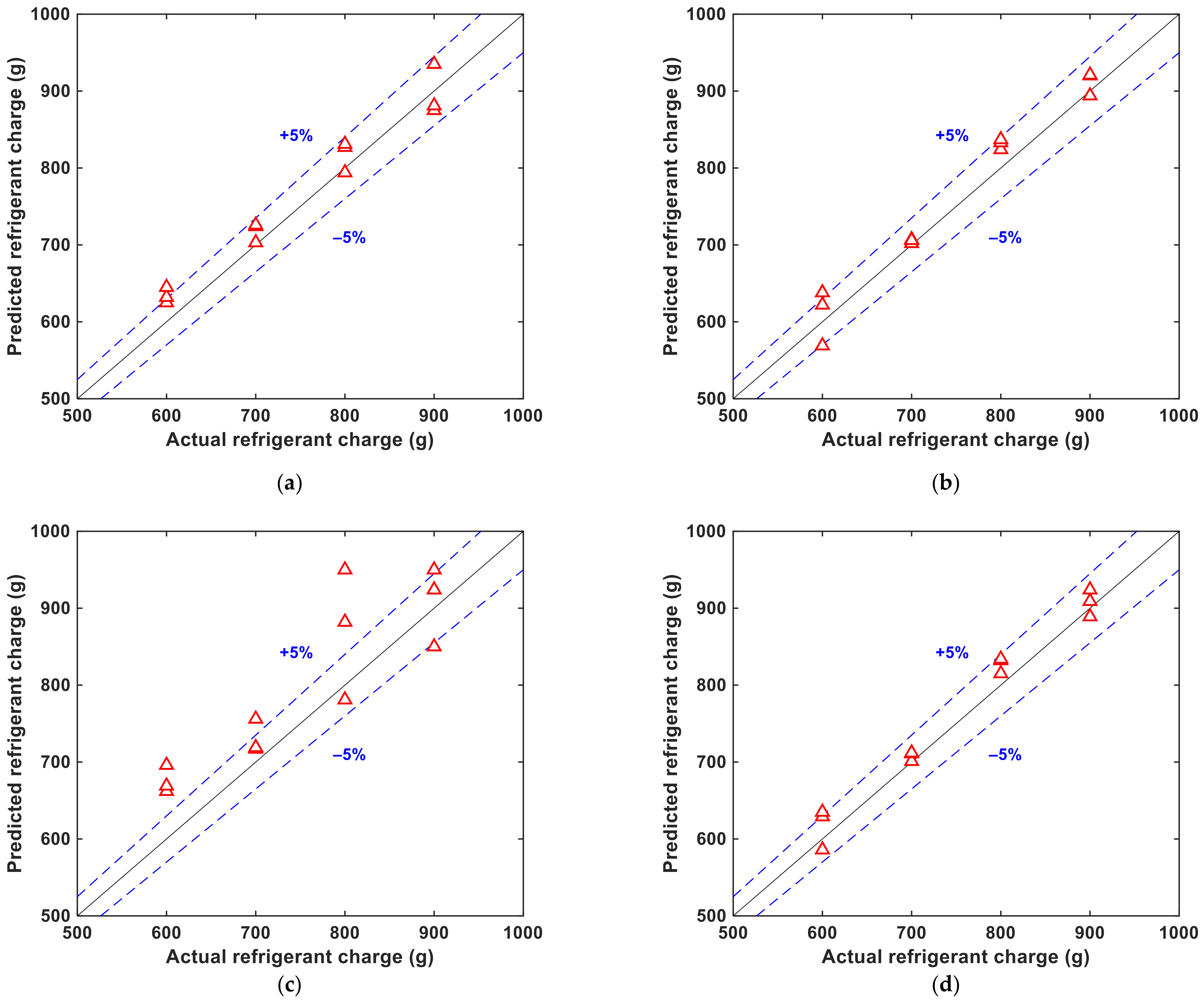
The refrigerant charge is one of the predictors that define the dynamic characteristics of response variables. When the refrigerant charge amount has not been specified, it can be estimated by measuring whether the response values of the dynamic model can reflect the experimental data well. The refrigerant charge amounts can be obtained by minimizing the RMSEs of the response values and test data for each response variable (Figure 10 and Table 5). For the four response variables in Table 5 and Figure 10, the refrigerant charge amount cannot be predicted with the compressor discharge temperature model. As shown in Figure 8, the dynamic characteristics at refrigerant charges of 750 g or more are not greatly different. Thus, the compressor discharge temperature was excluded because of the poor prediction, and a new combination including the condensation temperature and degree of subcooling variables was added. When each of the four models is used for the test data, the prediction results of the refrigerant charge amount are displayed with prediction errors, which are defined as the relative error percentages with respect to the deviation regarding the actual measured value and the predicted value.
When the condensation temperature model was used, the prediction error of the refrigerant charge amount was 3.3%; when the refrigerant charge amount was small, its predicted value tended to be higher. In addition, the prediction error increased with increasing refrigerant charge amount. When the degree of subcooling model was used, the prediction error was 2.8%.
When the power consumption model was used, the prediction result for the refrigerant charge amount was very poor. Its prediction was difficult at 800 and 900 g near the rated refrigerant charge amounts because the dynamic characteristics of the power consumption were similar at different charge levels.
Moreover, the prediction errors of the condensation temperature and degree of subcooling with respect to the refrigerant charge showed opposite trends. Thus, the condensation temperature and degree of subcooling models were combined to estimate the refrigerant charge. By using the RMSE in Equation (5), the refrigerant charge amount that minimizes the RMSEs of the two response variables (i.e., the condensation temperature and degree of subcooling) can be obtained (Figure 10d and Table 5):
When the condensation temperature and degree of subcooling models were combined, the prediction error was 2.54%; thus, the prediction performance was improved compared to when the condensation temperature and subcooling models were used alone. In particular, the prediction error was reduced in the case of 600 g, which resulted in the lowest prediction performance.
When developing a data-driven model using machine learning technique, a new model should be developed depending on the target system or if the regulation parameters of the system change in principle. However, it is expected that the SVM technique, variables selection, and diagnosis methodology presented in this paper can be applied to similar air conditioner systems.
6. Conclusions
In this study, the start-up characteristics of an air conditioner were analyzed according to the refrigerant charge amount under various operating conditions. In addition, dynamic models for the start-up characteristics were developed with r-SVM and used to create a prediction method for the refrigerant charge amount. The following important results were obtained:
- The changes in the dynamic characteristics according to the refrigerant charge amount during the start-up of an air conditioner can be monitored.
- The dynamic models for the condensation temperature and degree of subcooling can predict the distinct start-up characteristics that depend on the refrigerant charge amount. The estimated RMSEs of the condensation temperature and degree of subcooling of the test data are 0.53 and 0.84 °C, respectively.
- The refrigerant charge is one of predictors that define the dynamic characteristics of response variables. The refrigerant charge can be estimated by minimizing the RMSEs of the predicted values of the dynamic model and experimental data.
- The proposed method, which uses the dynamic model during start-up operation, is an effective technique for predicting the refrigerant charge amount. The average prediction error for the test data is 2.54%.
Author Contributions
Experiment, analysis, and writing—original draft preparation, Y.Y.; supervision, writing—review and editing, Y.S.C. All authors have read and agreed to the published version of the manuscript.
Funding
This research was conducted with the funding of the government (Ministry of Science and ICT) and with the support of the National Research Foundation of Korea (NRF-2019R1F1A1062125).
Institutional Review Board Statement
Not applicable.
Informed Consent Statement
Not applicable.
Data Availability Statement
Data sharing not applicable.
Conflicts of Interest
The authors declare no conflict of interest.
Nomenclature
| Symbols | |
| b | bias (scalar parameter defining decision boundary position) |
| Fcomp | frequency of compressor input power (Hz) |
| P | pressure (kPa) |
| Ref | refrigerant charge amount (g) |
| T | temperature (°C) |
| w | flatness (vector parameter defining decision boundary position) |
| W | power consumption (kW) |
| x | multivariate set of predictor |
| y | response variable |
| ϵ | maximal width of x and the decision boundary (hyper-parameter of model) |
| ξ, ξ* | slack variables (distance of the decision boundary and error data) |
| Abbreviations | |
| C | penalty constant (hyper-parameter of model) |
| COP | coefficient of performance |
| c | condenser |
| dis | discharge |
| e | evaporator |
| ex | electric expansion valve (EEV) |
| HX | heat exchanger |
| ID | indoor unit |
| in | inlet |
| iqr | interquartile |
| m | number of response variables |
| meas | measured |
| n | number of data sample |
| OD | outdoor unit |
| pred | prediction |
| RMSE | root mean square error |
| r-SVM | regression support vector machine |
| s | saturation temperature |
| sat | saturation |
| sc | subcooling |
| suc | suction |
References
- US Energy Information Administration. Annual Energy Outlook 2017; US Energy Information Administration: Washington, DC, USA, 2017.
- Srinivas, K.; Michael, R.B. Review Article: Methods for fault detection, diagnostics, and prognostics for building systems―A review, part I. HVAC&R Res. 2005, 11, 3–25. [Google Scholar]
- Madani, H.; Roccatello, E. A comprehensive study on the important faults in heat pump system during the warranty period. Int. J. Refrig. 2014, 48, 19–25. [Google Scholar] [CrossRef]
- Choi, J.M.; Kim, Y.C. The effects of improper refrigerant charge on the performance of a heat pump with an electronic expansion valve and capillary tube. Energy 2002, 27, 391–404. [Google Scholar] [CrossRef]
- Kim, D.H.; Park, H.S.; Kim, M.S. The effect of the refrigerant charge amount on single and cascade cycle heat pump systems. Int. J. Refrig. 2014, 40, 254–268. [Google Scholar] [CrossRef]
- Kim, N.H. Optimization of the water spray nozzle, refrigerant charge amount and expansion valve opening for a unitary ice maker using R-404A. Int. J. Air Cond. Refrig. 2017, 25, 1750025. [Google Scholar] [CrossRef]
- Goswami, D.Y.; Ek, G.; Leung, M.; Jotshi, C.K.; Sherif, S.A.; Colacino, F. Effect of refrigerant charge on the performance of air conditioning systems. Int. J. Refrig. 2001, 25, 741–750. [Google Scholar] [CrossRef]
- Farzad, M.; O’Neal, D.L. System performance characteristics of an air conditioner over a range of charging conditions. Int. J. Refrig. 1991, 14, 321–328. [Google Scholar] [CrossRef]
- Rodrigo, L.; Daniel, C.A.; Angelo, M.; Laura, N.A.; Ramon, C. TEWI analysis of a stand-alone refrigeration system using low-GWP fluids with leakage ratio consideration. Int. J. Refrig. 2020, 118, 279–289. [Google Scholar]
- Tassou, S.A.; Grace, I.N. Fault diagnosis and refrigerant leak detection in vapour compression refrigeration systems. Int. J. Refrig. 2005, 28, 680–688. [Google Scholar] [CrossRef]
- Rossi, T.M.; Braun, J.E. A statistical, rule-based fault detection and diagnostic method for vapor compression air conditioners. HVAC&R Res. 1997, 3, 19–37. [Google Scholar]
- Kocyigit, N.; Bulgurcu, H.; Lin, C.X. Fault diagnosis of a vapor compression refrigeration system with hermetic reciprocating compressor based on p-h diagram. Int. J. Refrig. 2014, 45, 44–54. [Google Scholar] [CrossRef]
- Grace, I.N.; Datta, D.; Tassou, S.A. Sensitivity of refrigeration system performance to charge levels and parameters for on-line leak detection. Appl. Therm. Eng. 2005, 25, 557–566. [Google Scholar] [CrossRef]
- Li, G.; Hu, Y.; Chen, H.; Shen, L.; Li, H.; Li, J.; Hu, W. Extending the virtual refrigerant charge sensor(VRC) for variable refrigerant flow (VRF) air conditioning system using data-based analysis methods. Appl. Therm. Eng. 2016, 93, 908–919. [Google Scholar] [CrossRef]
- Li, H.; Braun, J.E. Development, evaluation, and demonstration of a virtual refrigerant charge sensor. HVAC&R Res. 2009, 15, 117–136. [Google Scholar] [CrossRef]
- Li, H.; Braun, J.E. Virtual refrigerant pressure sensors for use in monitoring and fault diagnosis of vapor compression equipment. HVAC&R Res. 2009, 15, 597–616. [Google Scholar] [CrossRef]
- Li, B.; Alleyne, A.G. A dynamic model of a vapor compression cycle with shut-down and start-up operations. Int. J. Refrig. 2010, 33, 538–552. [Google Scholar] [CrossRef]
- Li, J.; Deng, W.; Yan, G. Improving quick cooling performance of a R410A split air conditioner during startup by actively controlling refrigerant mass migration. Appl. Therm. Eng. 2018, 128, 141–150. [Google Scholar] [CrossRef]
- Kim, M.; Kim, M.S. Performance investigation of a variable a vapor compression system for fault detection and diagnosis. Int. J. Refrig. 2005, 28, 481–488. [Google Scholar] [CrossRef]
- Elsayed, A.O.; Kayed, T.S. Dynamic performance analysis of inverter-driven split air conditioner. Int. J. Refrig. 2020, 118, 443–452. [Google Scholar] [CrossRef]
- Yoo, J.W.; Hong, S.B.; Kim, M.S. Refrigerant leakage detection in an EEV installed residential air conditioner with limited sensor installations. Int. J. Refrig. 2017, 78, 157–165. [Google Scholar] [CrossRef]
- Liu, J.; Hu, Y.; Chen, H.; Wang, J.; Li, G.; Hu, W. A refrigerant charge fault detection method for variable refrigerant flow (VRF) air-conditioning systems. Appl. Therm. Eng. 2016, 107, 284–293. [Google Scholar] [CrossRef]
- Kocyigit, N. Fault and sensor error diagnostic strategies for a vapor compression refrigeration system by using fuzzy inference systems and artificial neural network. Int. J. Refrig. 2015, 50, 69–79. [Google Scholar] [CrossRef]
- Shi, S.; Li, G.; Chen, H.; Liu, J.; Hu, Y.; Xing, L. Refrigerant charge fault diagnosis in the VRF system using bayesian artificial neural network combined with Relief filter. Appl. Therm. Eng. 2017, 112, 698–706. [Google Scholar] [CrossRef]
- Guo, Y.; Li, G.; Chen, H.; Wang, J.; Guo, M.; Sun, S. Optimized neural network-based fault diagnosis strategy for VRF system in heating mode using data mining. Appl. Therm. Eng. 2017, 125, 1402–1413. [Google Scholar] [CrossRef]
- Guo, Y.; Tan, Z.; Chen, H.; Li, G.; Wang, J.; Huang, R. Deep learning-based fault diagnosis of variable refrigerant flow air-conditioning system for building energy saving. Appl. Energy 2018, 225, 732–745. [Google Scholar] [CrossRef]
- Eom, Y.H.; Yoo, J.W.; Hong, S.B.; Kim, M.S. Refrigerant charge fault detection method of air source heat pump system using convolutional neural network for energy saving. Energy 2019, 187, 115877. [Google Scholar] [CrossRef]
- Xi, X.C.; Poo, A.N.; Chou, S.K. Support vector regression model predictive control on a HVAC plant. Control. Eng. Pract. 2007, 15, 897–908. [Google Scholar] [CrossRef]
- Allison, S.; Bai, H.; Jayaraman, B. Wind estimation using quadcopter motion: A machine learning approach. Aerosp. Sci. Techmol. 2020, 98, 105699. [Google Scholar] [CrossRef] [Green Version]
- Mahdevari, S.; Torabi, S.R. Prediction of tunnel convergence using artificial neural networks. Tunn. Undergr. Space Technol. 2012, 28, 218–228. [Google Scholar] [CrossRef]
- Burges, C.J. A tutorial on support vector machines for pattern recognition. Data Min. Knowl. Discov. 1998, 2, 121–167. [Google Scholar] [CrossRef]
- Cortes, C.; Vapnik, V. Support vector networks. Mach. Learn. 1995, 20, 273–297. [Google Scholar] [CrossRef]
- Smola, A.J.; Schlökopf, B. A tutorial on support vector regression. Stat. Comput. 2004, 14, 199–222. [Google Scholar] [CrossRef] [Green Version]
- Pai, P.F. System reliability forecasting by support vector machines with genetic algorithms. Math. Comput. Model. 2005, 43, 262–274. [Google Scholar] [CrossRef]
- Gunn, S.R. Support Vector Machines for Classification and Regression; Technical Report; University of Southampton: Southampton, UK, 1998. [Google Scholar]
- Hsu, C.W.; Chang, C.C.; Lin, C.J. A Practical Guide to Support Vector Classification; Technical Report; Department of Computer Science and Information Engineering, National Taiwan University: Taipei City, Taiwan, 2010. [Google Scholar]
- Bengio, Y.; Grandvalet, Y. No unbiased estimator of the variance of K-Fold Cross Validation. J. Mach. Learn. Res. 2004, 5, 1089–1105. [Google Scholar]
- Mathworks Help Center Support Vector Machine Regression. Available online: https://kr.mathworks.com/help/stats/support-vector-machine-regression.html?lang=en (accessed on 4 January 2021).
Figure 1.
Schematic diagram of experimental equipment.

Figure 2.
Positions of thermocouples for measuring heat exchanger temperature; (a) Condenser, (b) Evaporator.
Figure 2.
Positions of thermocouples for measuring heat exchanger temperature; (a) Condenser, (b) Evaporator.

Figure 3.
Variation in compressor suction and discharge pressure with rated refrigerant charge.

Figure 4.
Temperature distribution in heat exchanger with rated refrigerant charge; (a) Condenser, (b) Evaporator.
Figure 4.
Temperature distribution in heat exchanger with rated refrigerant charge; (a) Condenser, (b) Evaporator.

Figure 5.
Variation in condensation temperature over time with refrigerant charge amount.

Figure 6.
Variation in degree of subcooling over time with refrigerant charge amount.

Figure 7.
Variation in evaporation temperature over time with refrigerant charge amount.

Figure 8.
Variation in compressor discharge temperature over time with refrigerant charge amount.

Figure 9.
Prediction results of dynamic characteristic for each parameter using test data: (a) condensation temperature; (b) degree of subcooling; (c) compressor discharge temperature; (d) power sonsumption.
Figure 9.
Prediction results of dynamic characteristic for each parameter using test data: (a) condensation temperature; (b) degree of subcooling; (c) compressor discharge temperature; (d) power sonsumption.

Figure 10.
Detection results of refrigerant charge amount for each model using test data: (a) condensation temperature; (b) degree of subcooling; (c) power consumption; (d) combination of condensation temperature and degree of subcooling models.
Figure 10.
Detection results of refrigerant charge amount for each model using test data: (a) condensation temperature; (b) degree of subcooling; (c) power consumption; (d) combination of condensation temperature and degree of subcooling models.


Table 1.
Measured parameters.
| Variable | Description | Unit |
|---|---|---|
| Ref | Refrigerant charge amount | g |
| Fcomp | Frequency of compressor input power | Hz |
| TID,in | Indoor unit—inlet air temperature | °C |
| TOD,in | Outdoor unit—inlet air temperature | °C |
| W | Power consumption | kW |
| Psuc | Compressor suction pressure | kPa |
| Pdis | Compressor discharge pressure | kPa |
| TID,out | Indoor unit—outlet air temperature | °C |
| TOD,out | Outdoor unit—outlet air temperature | °C |
| Tsuc | Compressor suction refrigerant temperature | °C |
| Tdis | Compressor discharge refrigerant temperature | °C |
| Tex,in | EEV refrigerant inlet temperature | °C |
| Tex,out | EEV refrigerant outlet temperature | °C |
| Tc,in | Condenser refrigerant inlet temperature | °C |
| Tc,sat | Condensation temperature | °C |
| Tc,out | Condenser refrigerant outlet temperature | °C |
| Tsc | Degree of subcooling (Tc,sat − Tc,out) | °C |
| Te,in | Evaporator refrigerant inlet temperature | °C |
| Te,sat | Evaporation temperature | °C |
| Te,out | Evaporator refrigerant outlet temperature | °C |
Table 2.
Experimental condition.
| No. | Outdoor Temperature | Initial Indoor Temperature | Refrigerant Charge Amount (g) | Charge Uncertainty (%) | Type |
|---|---|---|---|---|---|
| 1 | 30 | 28 | 550 | 0.91 | Training |
| 2 | 35 | 28 | 550 | 0.91 | Training |
| 3 | 40 | 28 | 550 | 0.91 | Training |
| 4 | 45 | 28 | 550 | 0.91 | Training |
| 5 | 35 | 35 | 550 | 0.91 | Training |
| 6 | 40 | 35 | 550 | 0.91 | Training |
| 7 | 45 | 35 | 550 | 0.91 | Training |
| 8 | 35 | 35 | 600 | 0.83 | Test |
| 9 | 40 | 35 | 600 | 0.83 | Test |
| 10 | 45 | 35 | 600 | 0.83 | Test |
| 11 | 30 | 28 | 650 | 1.09 | Training |
| 12 | 35 | 28 | 650 | 1.09 | Training |
| 13 | 40 | 28 | 650 | 1.09 | Training |
| 14 | 45 | 28 | 650 | 1.09 | Training |
| 15 | 35 | 35 | 650 | 1.09 | Training |
| 16 | 40 | 35 | 650 | 1.09 | Training |
| 17 | 45 | 35 | 650 | 1.09 | Training |
| 18 | 35 | 35 | 700 | 1.01 | Test |
| 19 | 40 | 35 | 700 | 1.01 | Test |
| 20 | 45 | 35 | 700 | 1.01 | Test |
| 21 | 30 | 28 | 750 | 1.33 | Training |
| 22 | 35 | 28 | 750 | 1.33 | Training |
| 23 | 40 | 28 | 750 | 1.33 | Training |
| 24 | 45 | 28 | 750 | 1.33 | Training |
| 25 | 35 | 35 | 750 | 1.33 | Training |
| 26 | 40 | 35 | 750 | 1.33 | Training |
| 27 | 45 | 35 | 750 | 1.33 | Training |
| 28 | 35 | 35 | 800 | 1.25 | Test |
| 29 | 40 | 35 | 800 | 1.25 | Test |
| 30 | 45 | 35 | 800 | 1.25 | Test |
| 31 | 30 | 28 | 850 | 1.44 | Training |
| 32 | 35 | 28 | 850 | 1.44 | Training |
| 33 | 40 | 28 | 850 | 1.44 | Training |
| 34 | 45 | 28 | 850 | 1.44 | Training |
| 35 | 35 | 35 | 850 | 1.44 | Training |
| 36 | 40 | 35 | 850 | 1.44 | Training |
| 37 | 45 | 35 | 850 | 1.44 | Training |
| 38 | 35 | 35 | 900 | 1.36 | Test |
| 39 | 40 | 35 | 900 | 1.36 | Test |
| 40 | 45 | 35 | 900 | 1.36 | Test |
| 41 | 30 | 28 | 950 | 1.49 | Training |
| 42 | 35 | 28 | 950 | 1.49 | Training |
| 43 | 40 | 28 | 950 | 1.49 | Training |
| 44 | 45 | 28 | 950 | 1.49 | Training |
| 45 | 35 | 35 | 950 | 1.49 | Training |
| 46 | 40 | 35 | 950 | 1.49 | Training |
| 47 | 45 | 35 | 950 | 1.49 | Training |
Table 3.
Parameters.
| Response Variable | Predictors |
|---|---|
| Tc,sat | Ref, , TOD,in, TID,in, , |
| Tsc (Tc,sat − Tc,out) | Ref, , TOD,in, TID,in, , |
| Tdis | Ref, , TOD,in, TID,in, , |
| W | Ref, , TOD,in, TID,in, , |
Table 4.
Optimized parameters of support vector machine (SVM) in grid search.
| Kernel | K-Fold | Response Variable | C | RMSE | ||
|---|---|---|---|---|---|---|
| Training Data | Test Data | |||||
| Linear | 5 | Tc,sat | 0.509 | 0.101 | 0.51 °C | 0.53 °C |
| Tsc | 0.414 | 0.076 | 0.83 °C | 0.84 °C | ||
| Tdis | 0.461 | 0.301 | 3.76 °C | 5.12 °C | ||
| W | 20.3 | 29.8 | 5.54% | 5.6% | ||
Table 5.
Refrigerant charge detection accuracy.
| Response Variable | Refrigerant Charge Amount (g) | Error (%) | Average Error (%) | |
|---|---|---|---|---|
| Actual | Detected | |||
| Tc,sat | 600 | 625/632/645 | 5.7 | 3.32 |
| 700 | 703/724/726 | 2.5 | ||
| 800 | 794/827/831 | 2.7 | ||
| 900 | 875/881/935 | 2.9 | ||
| Tsc | 600 | 569/622/638 | 4.9 | 2.79 |
| 700 | 702/706/707 | 0.7 | ||
| 800 | 824/833/837 | 3.9 | ||
| 900 | 894/920/921 | 1.8 | ||
| W | 600 | 662/669/696 | 13.3 | 7.3 |
| 700 | 717/719/756 | 4.4 | ||
| 800 | 781/882/950 | 10.2 | ||
| 900 | 850/924/950 | 4.6 | ||
| Tc,sat and Tsc | 600 | 586/629/635 | 3.9 | 2.54 |
| 700 | 701/711/712 | 1.1 | ||
| 800 | 815/832/834 | 3.5 | ||
| 900 | 889/909/924 | 1.7 | ||
Publisher’s Note: MDPI stays neutral with regard to jurisdictional claims in published maps and institutional affiliations. |
© 2021 by the authors. Licensee MDPI, Basel, Switzerland. This article is an open access article distributed under the terms and conditions of the Creative Commons Attribution (CC BY) license (http://creativecommons.org/licenses/by/4.0/).
Share and Cite
MDPI and ACS Style
Yun, Y.; Chang, Y.S. Refrigerant Charge Prediction of Vapor Compression Air Conditioner Based on Start-Up Characteristics. Appl. Sci. 2021, 11, 1780. https://doi.org/10.3390/app11041780
AMA Style
Yun Y, Chang YS. Refrigerant Charge Prediction of Vapor Compression Air Conditioner Based on Start-Up Characteristics. Applied Sciences. 2021; 11(4):1780. https://doi.org/10.3390/app11041780
Chicago/Turabian StyleYun, Yechan, and Young Soo Chang. 2021. "Refrigerant Charge Prediction of Vapor Compression Air Conditioner Based on Start-Up Characteristics" Applied Sciences 11, no. 4: 1780. https://doi.org/10.3390/app11041780
Note that from the first issue of 2016, this journal uses article numbers instead of page numbers. See further details here.