
Stiffness Estimation and Equivalence of Boundary Conditions in FEM Models


1
Faculty of Mechanical Engineering, Technical University of Košice, 042 00 Košice, Slovakia
2
Faculty of Mechanical Engineering, Technical University of Ostrava, 708 00 Ostrava, Czech Republic
*
Author to whom correspondence should be addressed.
Appl. Sci. 2021, 11(4), 1482; https://doi.org/10.3390/app11041482
Submission received: 17 January 2021
/
Revised: 26 January 2021
/
Accepted: 3 February 2021
/
Published: 6 February 2021
(This article belongs to the Special Issue Uncertainty Analysis of Mechanical Systems)
Abstract
:The paper deals with methods of equivalence of boundary conditions in finite element models that are based on finite element model updating technique. The proposed methods are based on the determination of the stiffness parameters in the section plate or region, where the boundary condition or the removed part of the model is replaced by the bushing connector. Two methods for determining its elastic properties are described. In the first case, the stiffness coefficients are determined by a series of static finite element analyses that are used to obtain the response of the removed part to the six basic types of loads. The second method is a combination of experimental and numerical approaches. The natural frequencies obtained by the measurement are used in finite element (FE) optimization, in which the response of the model is tuned by changing the stiffness coefficients of the bushing. Both methods provide a good estimate of the stiffness at the region where the model is replaced by an equivalent boundary condition. This increases the accuracy of the numerical model and also saves computational time and capacity due to element reduction.
1. Introduction
Numerical methods are a highly effective tool for solving complex problems in the field of structural mechanics, acoustics, fluid flow, heat transfer, mass transfer, electromagnetism, multiphysics, etc. They have become an integral part of the daily work of engineers, scientists and researchers. The finite element method (FEM) is the most widely used method of them.
The correctness of the numerical solution in the finite element method is largely dependent on the accuracy of the FE model itself. The basis is to correctly define material properties, initial conditions, loads, and boundary conditions such as constraints, connections, and contacts in accordance with the real ones. Any inaccuracies in the model definition lead to deviations or errors in the load response. In particular, dynamic problems, such as modal analysis [1,2], impact tests [3,4], and fatigue analyses [5,6], are quite sensitive to boundary conditions and material parameters. The most common causes of differences in model behavior may be constraint stiffness and structural damping [7,8]. Computational models are usually verified by correlating the results of numerical calculation and experimental measurement. A suitable approach is to compare modal parameters (i.e., natural frequencies and mode shapes), for example, using the Modal Assurance Criterion (MAC) [9,10,11]. In order to improve the FE model, it is then possible to perform a sensitivity analysis or an optimization analysis, where the response is adjusted by changing the input parameters or identifying them. This procedure is known as finite element model updating.
The finite element model updating procedure was introduced in the 1980s [12]. Its main purpose is to calibrate the FE model of an analyzed structure in an appropriate way in order to match numerical and experimental results. Based on the correlation of these results, it is possible to identify inaccuracies or determine unknown parameters in the initial finite element model, such as the material properties, boundary conditions, etc. From this point of view, the FE model updating is an inverse task. A number of FE model updating methods have been proposed. They can be divided into non-iterative (direct) methods and iterative methods. The direct methods update the elements of stiffness and mass matrices using the equations of motion and the orthogonality equations [13]. The iterative methods typically involve using the sensitivity of the parameters to find their changes [14]. They are usually posed as an optimization problem, in which an objective function represents the model error (i.e., the difference between the numerical and experimental response). Most of FE model updating methods are based on frequency response functions (FRFs) or modal parameters, which are usually determined by experimental or operational modal analysis. Therefore, they are referred to as vibration-based model updating methods.
The number of publications devoted to FE model updating proves that it is a robust tool widely used in many areas, including the design, mechanical engineering, civil engineering, automotive, aerospace, and so on. In addition to refining FE models, it can also be used for system parameter identification, damage detection, health monitoring, structural control, and to determine unknown or equivalent material properties.
Yang et al. [15] used the model updating method based on multi-objective optimization to identify joints parameters by approaching actual test results. Their methodology was successfully tested on the SUV frame with seam and spot welds. Meggitt and Moorhouse [16] proposed the method that is able to avoid the need to achieve an idealized boundary condition when performing experimental tests for model updating purposes. That is, the FE model updating can be achieved in the presence of an arbitrary or unknown boundary condition using in-situ measurements. The practical application was illustrated through an example, in which an FE model of a cylindrical rubber vibration isolator was updated using in-situ experimental data and sub-structure invariants without it being removed from an assembly. Since most of FE model updating techniques do not employ damping, Arora et al. [17] proposed a two-step procedure that is able to update mass and stiffness matrices and, subsequently, identify the damping matrix. It allows accurate prediction of complex frequency response functions. The effectiveness of the proposed procedure was demonstrated by numerical examples as well as by actual experimental data. Girardi et al. [18] presented the use of FE model updating in civil structural applications. They proposed the method tailored to the needs of structural FE analysis of large size models. Its basis is an efficient model reduction strategy derived by slightly modifying the Lanczos projection, which in combination with a trust-region method allows matching the measured frequencies with the ones predicted by the parametric model. The authors performed several numerical experiments aimed to determine the optimal values of Young’s modulus and the mass density of building materials.
The FE model updating can also be applied on composite materials. Panvar et al. provided a detailed overview of this topic [19]. In the case of composite structures, the response is highly dependent on the orientation of the fibers and the material properties of all constituents. Maljaars et al. [20] developed an inverse method that minimizes the residual between the experimental and numerical results by adapting the stiffness properties in the FE calculation. The method is based on static tests and allows correct modelling of the fiber orientations and material properties. It was used to improve the structural response of two small scale marine composite propeller. The accuracy of the results was verified by comparing the natural frequencies. Zhao et al. [21] proposed a multi-level optimization approach for updating finite element models, in which the mass and stiffness related parameters are updated, respectively, in two different levels. The approach was employed for updating the finite element models of a composite flying-wing aircraft by using experimental results for both the aircraft and its components. The optimization results showed that the component responses may not match the test data when only using the test data for the complete model. When integrating the components’ test data in the FE model updating, the responses for both the complete model and the components match the test data well. In their study [22], He et al. focused on the assessment of a set of reliable composite material constitutive parameters, which are extracted using digital image correlation (DIC) and FE model updating. The uncertainty was induced by the measurement system noise in the DIC technique and the approximation error in the displacements and strains smoothing algorithm.
Another problem where the FE model updating can be applied is the homogenization. Homogenization techniques allow to investigate the macroscopic behavior of a heterogeneous, porous or composite material, considering that the original material is replaced by an equivalent homogeneous material with comparable properties. Gnoli et al. [23] presented a simple approach to study a hollow cylinder composite beam as it behaves like an isotropic one. The stiffness matrix of the equivalent 3D Euler–Bernoulli beam model was obtained using the proposed analytical method. Using this approach, the authors investigated the behavior of beams with different laminate configurations. Dunaj et al. [24] performed the dynamic FE analysis of steel–polymer concrete beams, in which the highly heterogeneous polymer concrete was modelled as a linear isotropic material. Three models of beams differing in cross-sectional dimensions showed high agreement with experimentally obtained mode shapes and frequency response functions.
Another important application of the FE model updating is damage detection and structural health monitoring [25]. Madheswaran and Srinivas [26] presented a way to locate damages in a structure based on the changes in Young modulus that indicate the loss of stiffness at the crack location. Thus, in the model updating process the Young modulus is chosen as the updating parameter. The method is based on the correlation of the reference FE model which depicts the undamaged structure with the test data (natural frequencies and mode shapes) obtained by measuring on the damage structure. Reynders et al. used a similar approach to identify bridge damage in their case study [27]. In the procedure they have proposed, the reference FE model is updated using a model that can reproduce the experimental modal data of the damaged state. These data were obtained by OMAX method (i.e., output-only data are used when updating the FE model). The crack location is determined by correction factors that express the change in bending and torsional stiffness of the model.
This paper deal with procedures aimed at improving boundary conditions in the FE model. Conventional boundary conditions are usually defined as ideal. It is common practice that constraints in FE models are modelled as perfectly rigid, while in fact they have a certain degree of flexibility. Although this is acceptable in many cases, there are problems, such as vibration analysis, fatigue analysis, etc., in which it is necessary to obtain an accurate model response. The idealization of the boundary conditions can have a significant effect on the results and may cause them not to match the experimental test data. For this reason, an equivalence method is proposed to replace a conventional boundary condition or a certain part of the model. The equivalent boundary condition is represented by a bushing connector whose stiffness parameters can be determined either by a series of numerical static analyses or using the FE model updating. The updating method used in the paper is based on FE optimization analysis, in which the natural frequencies of the model are fitted to the frequencies determined by experimental modal analysis. The authors successfully used this approach to determine the material constants of the isotropic material [28], the homogenized laminate [29], and to determine the fiber orientation of the composite plate [30].
The use of the equivalence method allows to replace an ideal (perfectly rigid) boundary condition with a constraint of finite stiffness. The aim is to refine the model behavior in a given place and improve its response. The equivalent constraint can be modelled using a generalized spring element or a bushing connector. In this paper, the equivalence method is used to replace a part of the model. This requires determining stiffness at the point where the model is split. Two ways to determine equivalent stiffness coefficients are presented below. As will be shown, this approach provides a significant simplification of the FE model, while maintaining its dynamic behavior. The main benefit is then the shortening of the calculation time.
2. Equivalence Method Based on a Series of Static Analyses
The principle of this method is explained on the example of a beam whose one end is fixed to the base frame by means of two preloaded bolts. This part of the model will be replaced by a bushing connector, the stiffness coefficients of which will be determined by linear static FEM analysis. Subsequently, a modal analysis will be performed to compare the dynamic behaviors of the reference model and the simplified equivalent model. All FEM calculations described in this chapter were performed in the Abaqus/CAE 2017.
2.1. The Reference Model of the Beam
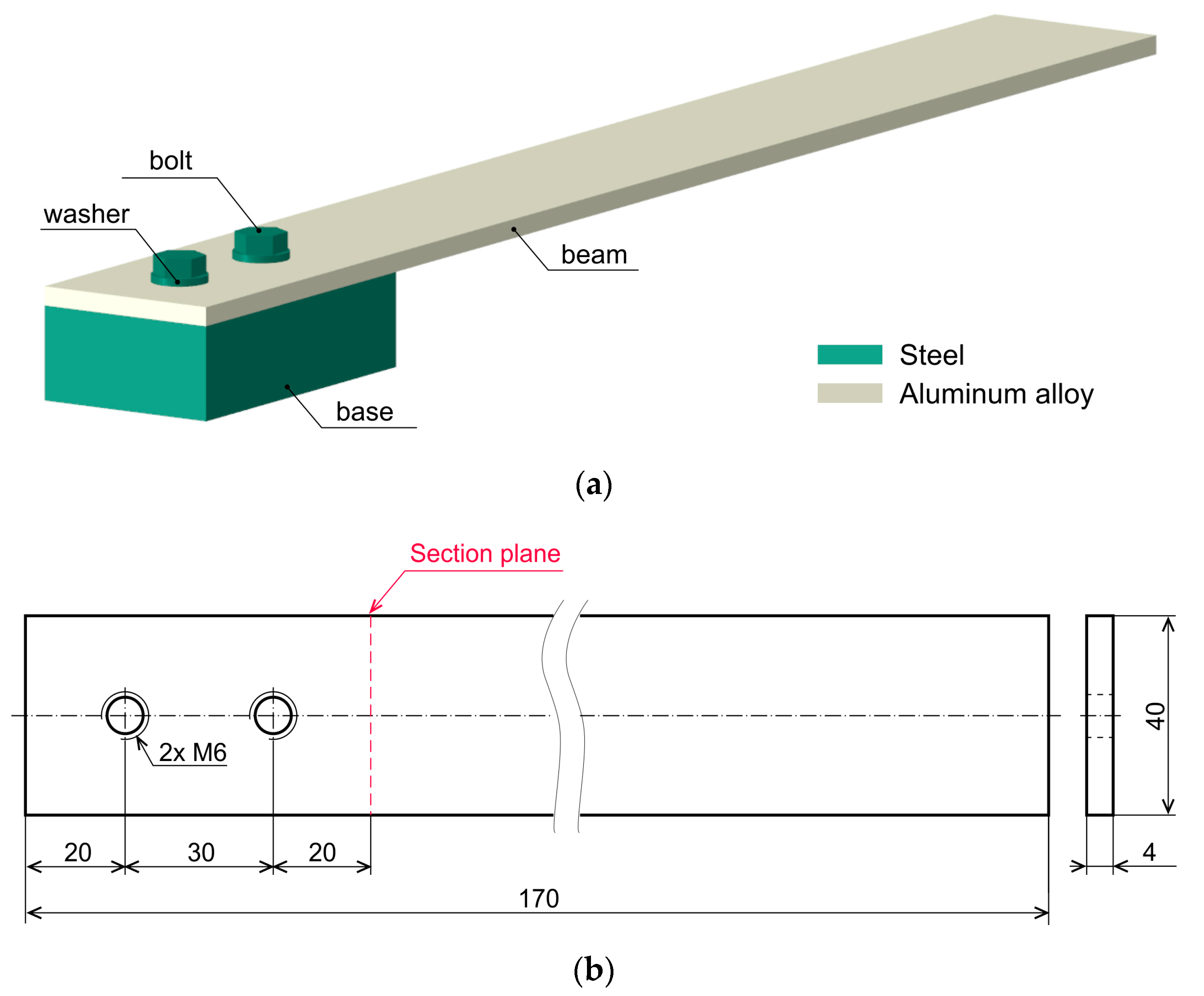
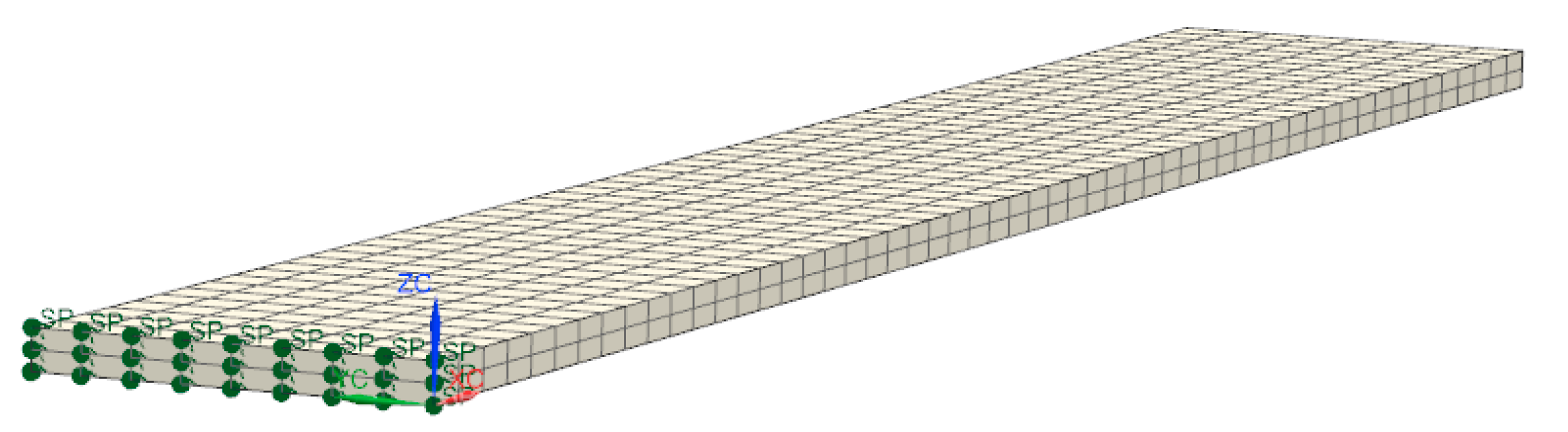
The reference model shown in Figure 1a consists of six parts: Beam with a rectangular cross section, base, two bolts M6 and two washers M6 × 12.5 mm. The beam is made of aluminum alloy. Its dimensions are shown in Figure 1b. Other components are made of steel. Note that all materials are considered isotropic and linear elastic in all FEM analyses performed. Their properties are listed in Table 1.
2.2. Equivalent Stiffness Coefficients Calculation
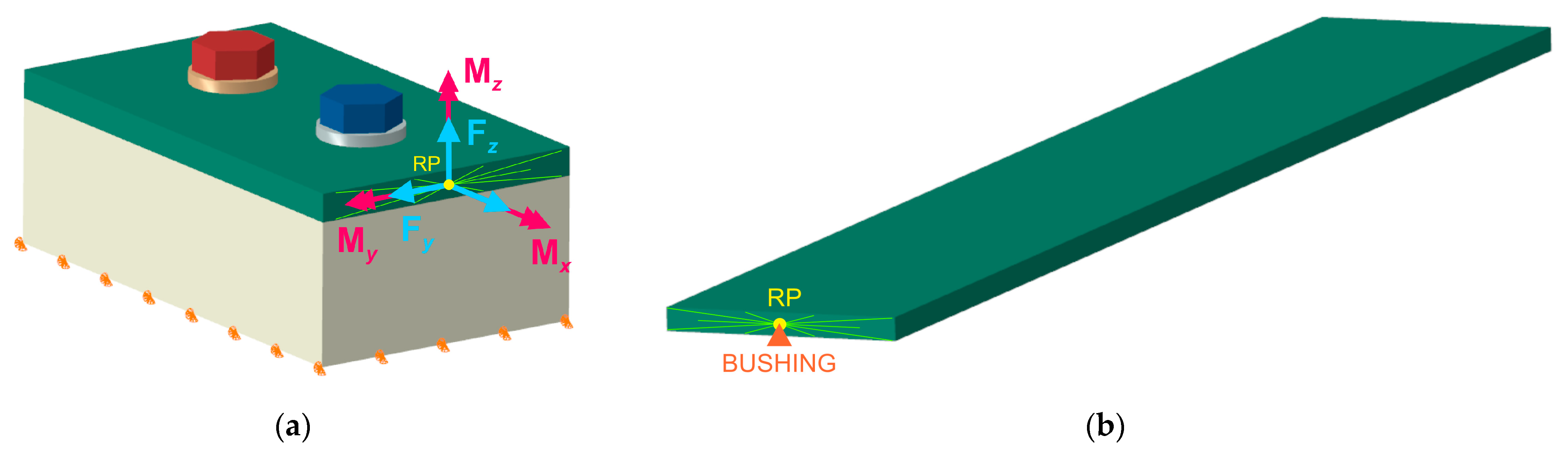
The red dashed line in Figure 1b shows a section plane in which part of the model is replaced by a bushing connector connected to ground. In Abaqus, connection type BUSHING provides a connection between two nodes that allows independent behavior in three local Cartesian directions and that allows different behavior in two flexural rotations and one torsional rotation. The equivalent FE model can be seen in Figure 2b. Figure 2a shows a separate (removed) part of the model that was used to calculate the stiffness coefficients of the bushing. These coefficients were determined by a series of six linear static analyses in which the residual part of the beam was loaded in all six degrees of freedom, respectively. The load was represented by a unit force and a unit moment acting at the reference point (RP). The transfer of the load from this point to the cross-sectional area of the beam was realized through a distribution coupling. In addition, the pretension was defined in the bolts. The preload force was set 10 kN. Since this is a contact task, frictional contact interactions were defined between all components. The friction coefficient was set to 0.2. In the normal direction, so-called hard contact was enforced. The underside of the base was fixed. The finite element mesh was formed by hexagonal elements with an average size of 1.5 mm.
The unknown stiffness coefficients of the bushing were calculated using the following formulas.
where , , are equivalent translational stiffness in x-, y-, z- direction, respectively; , , are maximum translations in x-, y-, z- direction, respectively; , , are loading forces acting in x-, y-, z- direction, respectively, and
where , , are equivalent rotational stiffness about x-, y-, z- axis, respectively; , , are maximum angular deflection about x-, y-, z- axis, respectively; , , are loading moments acting about x-, y-, z- axis, respectively.
2.3. Results and Discussion
The equivalent stiffness coefficients calculated by the above procedure were used in the definition of the bushing connector in the equivalent FE model. Their values are given in Table 2. The assumption of the equivalence method is that the finite element model modified in this way retains the stiffness properties of the original model and can therefore be used in further static or dynamic analyses. In order to verify this assumption, both FE models, the complete reference model (Figure 1a) and the equivalent model (Figure 2b), were subjected to modal analysis to assess their modal properties. A Lanczos eigensolver was used to calculate the natural frequencies and the modes shapes of the beam in the frequency range up to 5000 Hz.
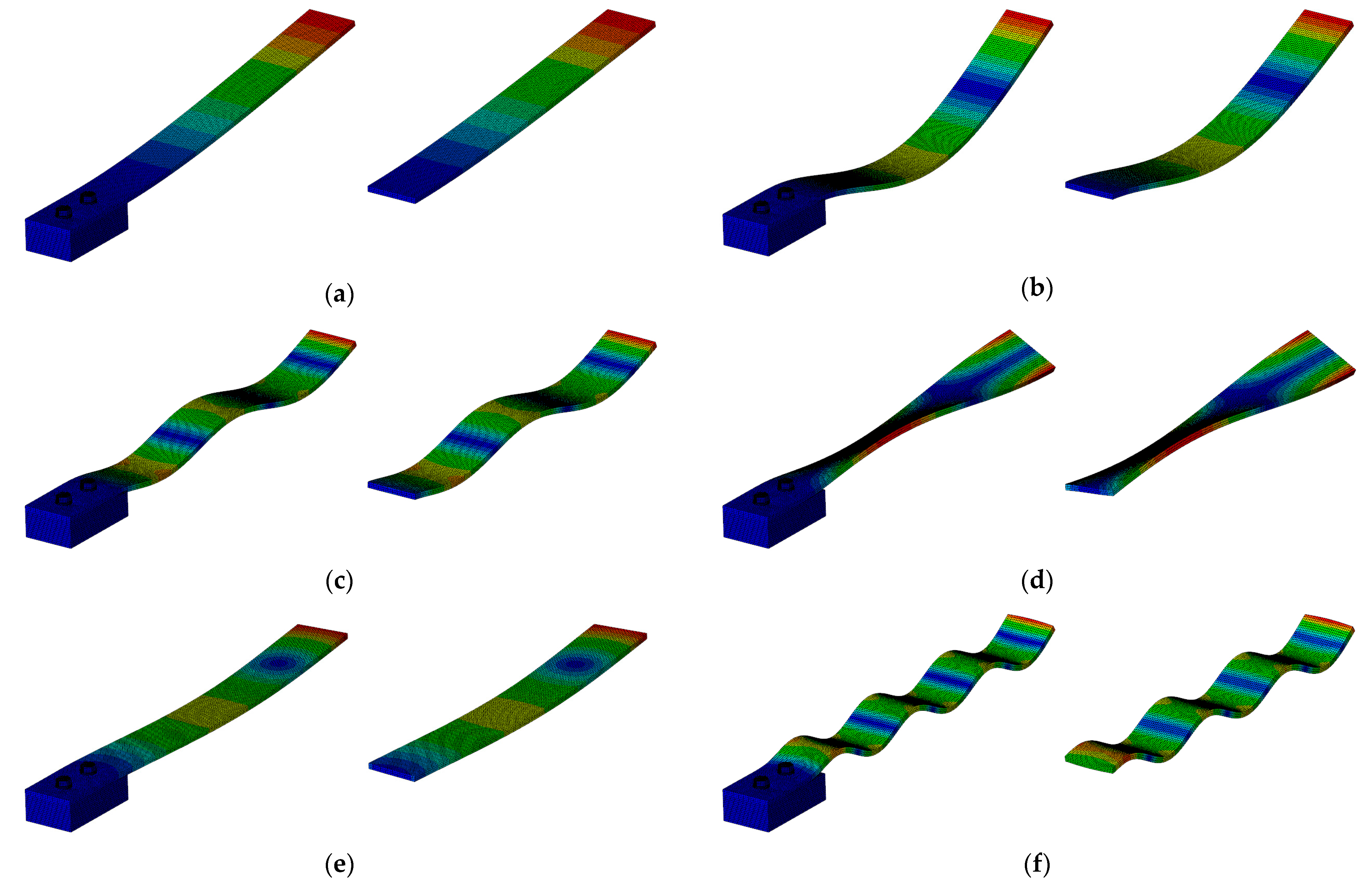
The natural frequencies of both models are compared in Table 3. Some corresponding mode shapes are shown in Figure 3. The results obtained show very good agreement. The natural frequency values of the equivalent model differ from the reference values in the range from −0.06% to 4.21%. The average percentage change is 1.33%. Negligible differences were also found for the mode shapes, which means that the equivalent model response corresponds to the response of the original complete model. In addition to maintaining dynamic behavior, the model was significantly simplified. The number of elements decreased from 59,747 to 15,148. Based on these findings, it can be concluded that the equivalence method works correctly.
3. Equivalence Method Based on Finite Element Model Updating
In this method, the stiffness coefficients are calculated based on the natural frequency values obtained by experimental modal analysis (EMA). The coefficients are determined in the parameter optimization process, which is based on frequency FEM analysis. By changing the stiffness of the bushing, the model is retuned, which is reflected in a change in its modal properties. During the optimization, the FE model is iteratively updated until its natural frequencies match the measured values with acceptable accuracy. It should be noted that the shape, dimensions, and material properties of the structure must be well known in advance. Flowchart of the updating process is shown in Figure 4.
3.1. Experimental Modal Analysis of the Beam
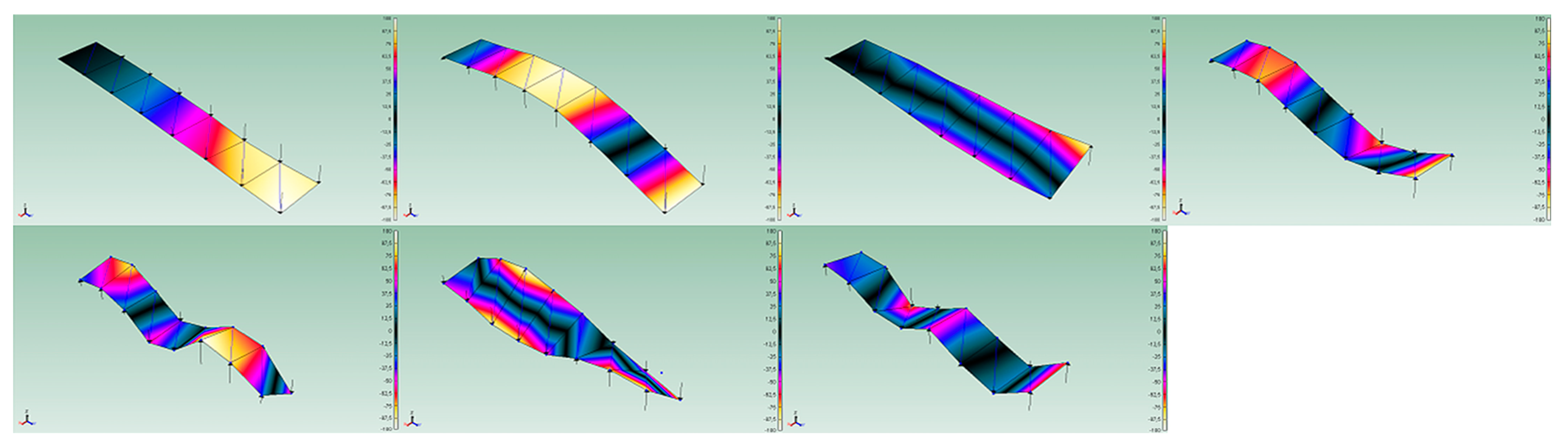
The proposed equivalence method is presented on a similar beam model as used in the previous case. The rectangular steel beam was fixed to the rigid base on one side by means of two bolt connections (Figure 4). Its natural frequencies and mode shapes were determined by a modal test, in which the beam was excited by impact hammer (Bruel and Kjaer type 8206) and its responses were measured by laser vibrometer (Polytec PDV100). Data acquisition was provided by the Pulse LAN-XI system. Modal parameters were extracted using Pulse Reflex software. The experimental setup is shown in Figure 5. In the frequency range up to 3.2 kHz, seven modes were identified, five of which are bending and two torsional (see Figure 6). The natural damped frequencies and damping ratios of these modes are listed in Table 4.
3.2. Equivalent Stiffness Coefficients Calculation
The parametric optimization was performed in NX Nastran software that uses gradient-based numerical optimization algorithm [31]. The equivalent FE model (Figure 7) consists only of the free part of the beam. The residual (removed) part of the structure was replaced by bushing elements connecting the section plane of the beam to the ground. The dimensions and material properties of the equivalent model are listed in Table 5.
Since NX allows only one objective function to be defined, the frequency of the first mode was set as the objective. Other frequencies were defined as optimization constraints with a tolerance of +/−5%. It should be noted that the lateral mode shapes of vibration were not identified by the modal test; however, they occur in FEM analysis (mode 3 and mode 8). For this reason, these modes have not been included among the optimization constraints. The coefficients , , representing the equivalent translational stiffness of the bushing in x-, y-, z- direction, respectively, were considered as the design variables.
The optimization parameters were defined as follows:
- Design Objective:Target Model Frequency Mode 1, Target value = 47.000 Hz
- Design Constraints:Model Frequency, Mode 1, Upper limit = 49.000 HzModel Frequency, Mode 1, Lower limit = 45.000 HzModel Frequency, Mode 2, Upper limit = 304.00 HzModel Frequency, Mode 2, Lower limit = 275.00 HzModel Frequency, Mode 4, Upper limit = 694.00 HzModel Frequency, Mode 4, Lower limit = 628.00 HzModel Frequency, Mode 5, Upper limit = 851.00 HzModel Frequency, Mode 5, Lower limit = 769.00 HzModel Frequency, Mode 6, Upper limit = 1645.0 HzModel Frequency, Mode 6, Lower limit = 1488.0 HzModel Frequency, Mode 7, Upper limit = 2098.0 HzModel Frequency, Mode 7, Lower limit = 1898.0 HzModel Frequency, Mode 9, Upper limit = 2690.0 HzModel Frequency, Mode 9, Lower limit = 2434.0 Hz
- Design Variables:kx (N/mm), Initial value = 6×10⁶, Lower limit = 500, Upper limit = 106ky (N/mm), Initial value = 6×10⁶, Lower limit = 500, Upper limit = 106kz (N/mm), Initial value = 6×10⁶, Lower limit = 500, Upper limit = 106
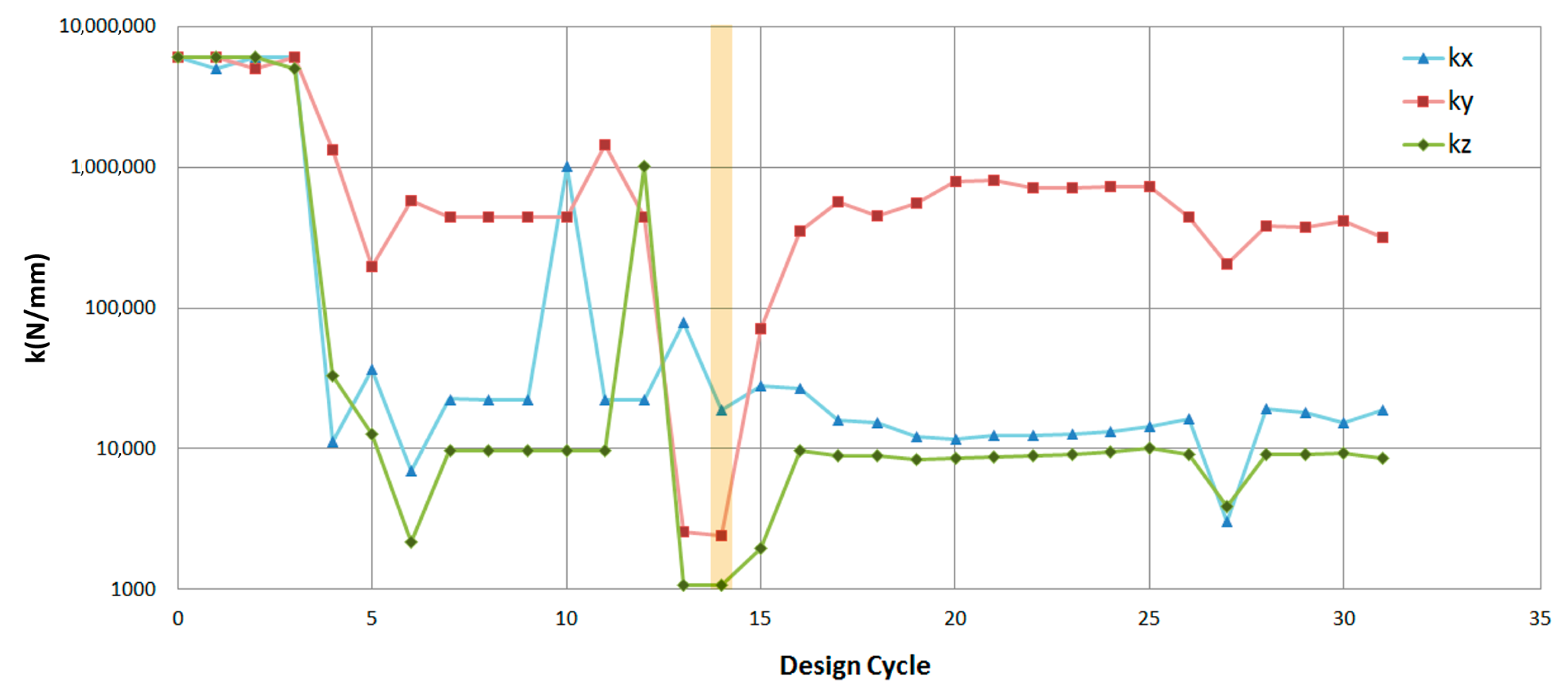
Figure 8 shows how the value of the objective function was changing in the individual optimization cycles. Figure 9 shows the changes of the design variables.
Since not all optimization constraints were met in any cycle, it was necessary to choose a solution where the estimate was closest to meeting them. In the 14. design cycle, five of the seven conditions were met; therefore, this cycle was considered to be the result of the optimization. Stiffness coefficients in this cycle were kx = 18,654.71 N/mm, ky = 2428.06 N/mm, kz = 1068.86 N/mm. These values were used in the definition of bushing in the final equivalent FE model.
3.3. Results and Discussion
The natural frequencies of this model are listed in Table 6. They are compared to measured frequencies that are considered as reference. Percentage deviations are calculated with respect to them. For interest, Table 6 also lists the frequencies of the cantilever beam model with ideal boundary conditions. The mode shapes of the final equivalent FE model can be seen in Figure 10.
The natural frequency values of the equivalent FE model differ from the reference values in the range from 0.56% to 7.35%. The average percentage deviation is 3.98%. However, it is evident that the equivalent FE model provides greater accuracy compared to the clamped beam model with a perfectly rigid constraint. Given that the torsional stiffness of the bushing was not taken into account when deriving the equivalent model, the results obtained can be considered acceptable. In addition, it should be recalled that the stiffness coefficients were not determined using multi-objective optimization.
4. Overview of Possible Applications of the Presented Methods
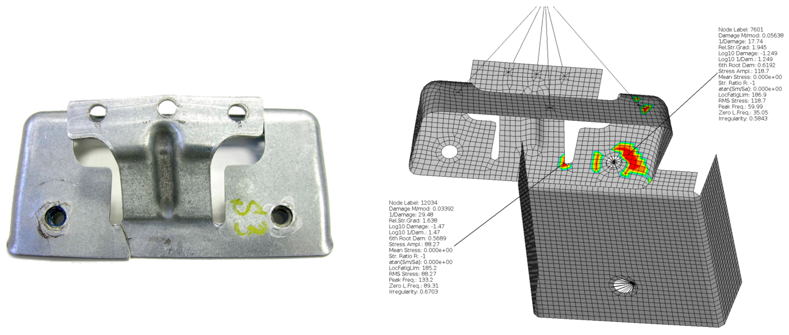
Many examples can be found in engineering practice, where instead of the whole model, only one of its components or subassemblies is analyzed. In such component tests, only ideal constraints are often used. This can, in some cases, lead to errors (e.g., in life prediction). In study [32] it was shown how problematic it is to calibrate a numerical model with ideal constraints so that the results of the fatigue analysis match the experimental data. The subject of the analysis was a car horn holder (Figure 11).
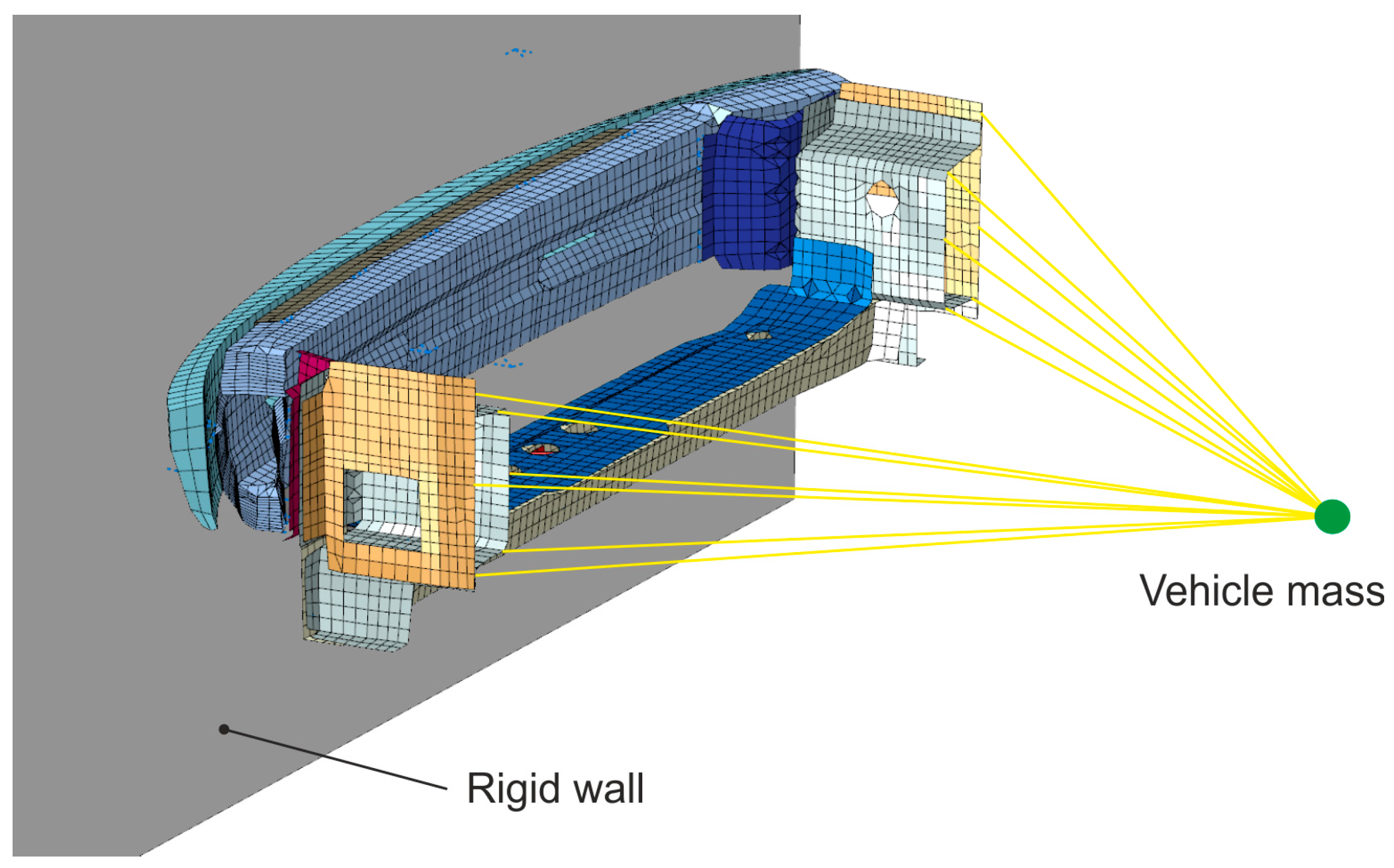
If the analysis is performed on a partial model, the neglected geometry is usually replaced by a point mass with inertial effects corresponding to the removed part. However, stiffness properties are ignored. A good example is the crash management system (CMS) of passenger cars, which is subjected to an impact test [33,34,35,36]. The CMS is a combination of conventional multi-chamber crashboxes and a bumper cross member. Crashboxes are attached to the so-called longitudinal members by means of connector plates. The longitudinal member establishes the main load path in the frontal crash scenarios. In the case of slow-speed impacts, they are usually not included to the model and the connector plates are coupled to a point mass replacing the rest of the vehicle, as shown in Figure 12.
5. Conclusions
In the paper, the methods of the equivalence of boundary conditions in the FE model were described. Their basis is the replacement of boundary condition, bond, constraint, or a part of the model by bushing or elastic connectors with corresponding stiffness. The paper presents two approaches to determine the stiffness parameters. The first method is based on a purely numerical calculation and is applicable when a real physical model does not exist. This approach is very accurate and effective. The second approach is based on the finite element model updating, where the stiffness parameters are determined using parametric optimization and modal analysis. The accuracy of this technique depends on several factors, such as natural frequencies, material properties, dimensions, and geometry of the structure, on the basis of which the FE model is created. From this point of view, it is an estimation method. However, the test results indicate that the estimate is relatively accurate and the procedure is practically applicable. It has also been shown that, in the case of replacing part of the model, the problem is significantly simplified, which is positively reflected in the shortening of the computational time.
While the first method is relatively simple and can be easily applied, the second method requires knowing the natural frequencies of the structure. These can be determined by experimental modal analysis. There are several measurement techniques that can be used for this purpose. In addition to conventional methods with accelerometers, advanced contactless optical methods can be used to perform either spot measurements or full-field measurements. Let us mention, for example, scanning laser Doppler vibrometry or high-speed digital image correlation. The advantage of experimental modal analysis is that it also provides information on structural damping. This can be used for advanced updating of FE models in dynamic analyses. In case more complex structures are analyzed, it is necessary to perform a multi-reference modal analysis to capture both global and local modes. If the structure is too complex to be measured effectively, the natural frequencies can be determined by numerical modal analysis. The weakness of the method is parametric optimization with one objective function. On the other hand, the accuracy of the method proved to be sufficient. In addition, the method has been shown to be applicable even if not all natural frequencies are included in the optimization process. From this point of view, this procedure for determining equivalent stiffness parameters can be helpful for CAE engineers and researchers who do not have advanced software for multi-objective optimization.
Author Contributions
Conceptualization, R.H.; data curation, P.L.; formal analysis, P.P. and J.M.; funding acquisition, R.H.; investigation, P.P. and A.K.; methodology, R.H. and P.L.; project administration, P.L.; resources, R.H. and P.L.; software, P.L. and A.K.; supervision, R.H.; validation, R.H.; visualization, A.K. and J.M.; writing—original draft, R.H. and P.P.; writing—review and editing, R.H. and P.L. All authors have read and agreed to the published version of the manuscript.
Funding
This work was supported by the Scientific Grant Agency of the Slovak Republic under grant VEGA 1/0355/18 and by Research and Development Operational Program funded by the ERDF within the project University Science Park TECHNICOM for Innovation Application Supported by Knowledge Technology, ITMS: 26220220182.
Institutional Review Board Statement
Not applicable.
Informed Consent Statement
Not applicable.
Data Availability Statement
Not applicable.
Conflicts of Interest
The authors declare no conflict of interest. The funders had no role in the design of the study; in the collection, analyses, or interpretation of data; in the writing of the manuscript, or in the decision to publish the results.
References
- Guan, C.; Zhang, H.; Wang, X.; Miao, H.; Zhou, L.; Liu, F. Experimental and Theoretical Modal Analysis of Full-SizedWood Composite Panels Supported on Four Nodes. Materials 2017, 10, 683. [Google Scholar] [CrossRef] [PubMed] [Green Version]
- Xia, B.; Liu, F.; Xu, C.; Liu, Y.; Lai, Y.; Zheng, W.; Wang, W. Experimental and Simulation Modal Analysis of a Prismatic Battery Module. Energies 2020, 13, 2046. [Google Scholar] [CrossRef]
- Ferreira, V.; Santos, L.P.; Franzen, M.; Ghouati, O.O.; Simoes, R. Improving FEM crash simulation accuracy through local thickness estimation based on CAD data. Adv. Eng. Softw. 2014, 71, 52–62. [Google Scholar] [CrossRef] [Green Version]
- Soni, S.; Pradhan, S.K. Improving crash worthiness and dynamic performance of frontal plastic automotive body components. Mater. Today Proc. 2020, 27, 2308–2313. [Google Scholar] [CrossRef]
- Kaľavský, A.; Huňady, R. Fatigue analysis of a notched beam in frequency domain. AIP Conf. Proc. 2019, 2198, 020007. [Google Scholar] [CrossRef]
- Kaľavský, A.; Huňady, R.; Kicko, M.; Kučinský, M. Calculation of the Fatigue Life of a Dynamically Loaded Component. Am. J. Mech. Eng. 2017, 5, 252–256. [Google Scholar]
- Goletti, M.; Mussi, V.; Rossi, A.; Monno, M. Procedures for Damping Properties Determination in Metal Foams to Improve FEM Modeling. Proc. Mater. Sci. 2014, 4, 233–238. [Google Scholar] [CrossRef] [Green Version]
- Iglesias, F.S.; López, A.F. Rayleigh damping parameters estimation using hammer impact tests. Mech. Syst. Signal. Proc. 2020, 135, 106391. [Google Scholar] [CrossRef]
- Siano, D.; Viscardi, M.; Aiello, R. Sensitivity Analysis and Correlation Experimental/Numerical FEM-BEM for Noise Reduction Assessment of an Engine Beauty Cover. Energy Proc. 2015, 81, 742–754. [Google Scholar] [CrossRef] [Green Version]
- Pastor, M.; Binda, M.; Harčarik, T. Modal Assurance Criterion. Proc. Eng. 2012, 48, 543–548. [Google Scholar] [CrossRef]
- Brehm, M.; Zabel, V.; Bucher, C. An automatic mode pairing strategy using an enhanced modal assurance criterion based on modal strain energies. J. Sound Vib. 2010, 329, 5375–5392. [Google Scholar] [CrossRef]
- Chen, J.C.; Garba, J.A. Analytical model improvement using modal test results. AIAA J. 1980, 18, 684–690. [Google Scholar] [CrossRef]
- Ren, W.X.; Chen, H.B. Finite element model updating in structural dynamics by using the response surface method. Eng. Struct. 2010, 32, 2455–2465. [Google Scholar] [CrossRef]
- Friswell, M.I.; Mottershead, J.E. Finite Element Model Updating in Structural Dynamics; Kluwer Academic Publishers: Amsterdam, The Netherlands, 1995. [Google Scholar]
- Yang, Y.; Chen, J.; Lan, F.; Xiong, F.; Zeng, Z. Joints Parameters Identification in Numerical Modeling of Structural Dynamics. Shock Vib. 2018, 9, 1–11. [Google Scholar] [CrossRef] [Green Version]
- Meggitt, J.W.R.; Moorhouse, A.T. Finite element model updating using in-situ experimental data. J. Sound Vib. 2020, 489, 2020. [Google Scholar] [CrossRef]
- Arora, V.; Singh, S.P.; Kundra, T.K. Finite element model updating with damping identification. J. Sound Vib. 2009, 324, 1111–1123. [Google Scholar] [CrossRef]
- Girardi, M.; Padovani, C.; Pellegrini, D.; Porcelli, M.; Robol, L. Finite element model updating for structural applications. J. Comput. Appl. Math. 2020, 370. [Google Scholar] [CrossRef] [Green Version]
- Panwar, V.; Gupta, P.; Bagha, A.K.; Chauhan, N. A Review on studies of Finite Element Model Updating and Updating of Composite Materials. Mater. Today Proc. 2018, 5, 27912–27918. [Google Scholar] [CrossRef]
- Maljaars, P.J.; Kaminski, M.L.; den Besten, J.H. Finite element modelling and model updating of small scale composite propellers. Compos. Struct. 2017, 176, 154–163. [Google Scholar] [CrossRef] [Green Version]
- Zhao, W.; Gupta, A.; Regan, C.D.; Miglani, J.; Kapania, R.K.; Seiler, P.J. Component data assisted finite element model updating of composite flying-wing aircraft using multi-level optimization. Aerosp. Sci. Technol. 2019, 95. [Google Scholar] [CrossRef]
- He, T.; Liu, L.; Makeev, A. Uncertainty analysis in composite material properties characterization using digital image correlation and finite element model updating. Compos. Struct. 2018, 184, 337–351. [Google Scholar] [CrossRef]
- Gnoli, D.; Babamohammadi, S.; Fantuzzi, N. Homogenization and Equivalent Beam Model for Fiber-Reinforced Tubular Profiles. Materials 2020, 13, 2069. [Google Scholar] [CrossRef] [PubMed]
- Dunaj, P.; Berczyński, S.; Chodźko, M.; Niesterowicz, B. Finite Element Modeling of the Dynamic Properties of Composite Steel–Polymer Concrete Beams. Materials 2020, 13, 1630. [Google Scholar] [CrossRef] [PubMed] [Green Version]
- Simoen, E.; De Roeck, G.; Lombaert, G. Dealing with uncertainty in model updating for damage assessment: A review. Mech. Syst. Signal. Proc. 2015, 56, 123–149. [Google Scholar] [CrossRef] [Green Version]
- Madheswaran, J.; Srinivas, V. Structural Damage Identification Based on Finite Element Model Updating. J. Mech. Eng. Autom. 2015, 5, 59–63. [Google Scholar] [CrossRef]
- Reynders, E.; Teughels, A.; De Roeck, G. Finite element model updating and structural damage identification using OMAX data. Mech. Syst. Signal. Proc. 2010, 24, 1306–1323. [Google Scholar] [CrossRef]
- Kaľavský, A.; Huňady, R.; Pavelka, P. Determining the young’s modulus of a specimen using experimental modal analysis. In Proceedings of the EAN 2018, Harrachov, Czech Republic, 5–7 June 2018; pp. 176–183. [Google Scholar]
- Huňady, R.; Pavelka, P.; Lengvarský, P. Homogenization of Material Properties of a Combined rubber/steel Sheet using Modal Analysis. In Proceedings of the EAN 2019, Luhacovice, Czech Republic, 3–6 June 2019; pp. 146–150. [Google Scholar]
- Huňady, R.; Pavelka, P.; Lengvarský, P.; Kaľavský, A. The estimation of elastic material constants of unidirectional fibre-reinforced composite based on modal analysis. In Proceedings of the MMaMS 2019, Sromowce Niżne, Poland, 11–13 September 2019; pp. 1–9. [Google Scholar]
- Design Sensitivity and Optimization User’s Guide (NX Nastran Help), Siemens. Available online: Docs.plm.automation.siemens.com/data_services/resources/nxnastran/10/help/en_US/tdocExt/pdf/optimization.pdf (accessed on 10 September 2020).
- Kaľavský, A. Design of a Methodology for Calculating the Fatigue Life under Random Loading Including Dynamic Behavior. Master Thesis, Technical University of Košice, Košice, Slovakia, 2017. (In Slovak). [Google Scholar]
- Koricho, E.; Belingardi, G.; Tekalign, A.; Roncato, D.; Martorana, B. Crashworthiness Analysis of Composite and Thermoplastic Foam Structure for Automotive Bumper Subsystem. In Advanced Composite Materials for Automotive Applications: Structural Integrity and Crashworthiness, 1st ed.; Elmarakbi, A., Ed.; John Wiley & Son Ltd.: Hoboken, NJ, USA; pp. 129–147.
- Constantin, B.A.; Iozsa, D.; Fratila, G. Studies about the Behavior of the Crash Boxes of a Car Body. IOP Conf. Series Mater. Sci. Eng. 2016, 161, 1–9. [Google Scholar] [CrossRef]
- Li, Z.; Yu, Q.; Zhao, X.; Yu, M.; Shi, P.; Yan, C. Crashworthiness and lightweight optimization to applied multiple materials and foam-filled front end structure of auto-body. Adv. Mech. Eng. 2017, 9, 1–21. [Google Scholar] [CrossRef]
- Beyene, A.T.; Koricho, E.G.; Belingardi, G.; Martorana, B. Design and manufacturing issues in the development of lightweight solution for a vehicle frontal bumper. Proc. Eng. 2014, 88, 77–84. [Google Scholar] [CrossRef] [Green Version]
- Basutkar, A.; Baruah, K.; Kudari, S.K. Frequency Analysis of Aircraft Wing Using FEM. In Recent Trends in Mechanical Engineering, 1st ed.; Narasimham, G., Babu, A., Reddy, S., Dhanasekaran, R., Eds.; Springer: Singapore, 2020; pp. 527–533. [Google Scholar]
- Chen, X.; Zha, G.; Yang, M. Numerical simulation of 3-D wing flutter with fully coupled fluid–structural interaction. Comput. Fluids 2007, 36, 856–867. [Google Scholar] [CrossRef]
- Venkatesan, S.P.; Beemkumar, N.; Jayaprabakar, J.; Kadiresh, P.N. Modelling and analysis of aircraft wing with and without winglet. Int. J. Ambient Energy 2018. [Google Scholar] [CrossRef]
- Ouyang, X.; Yu, X.; Wang, Y. Flutter analysis for wing structure using finite element modeling with equivalent stiffness. J. Vibroeng. 2014, 16, 1483–1493. [Google Scholar]
Figure 1.
(a) Reference model of the analyzed structure; (b) Dimensions of the beam.

Figure 2.
(a) Removed part of the model used to obtain the stiffness coefficients; (b) the equivalent model with bushing connector.
Figure 2.
(a) Removed part of the model used to obtain the stiffness coefficients; (b) the equivalent model with bushing connector.

Figure 3.
Selected mode shapes of compared FE models: (a) 1. mode; (b) 2. mode; (c) 6. mode; (d) 7. mode; (e) 8. mode; (f) 14. mode.
Figure 3.
Selected mode shapes of compared FE models: (a) 1. mode; (b) 2. mode; (c) 6. mode; (d) 7. mode; (e) 8. mode; (f) 14. mode.

Figure 4.
Flowchart of the updating process.

Figure 5.
Experimental modal analysis of the beam.

Figure 6.
Mode shapes of the beam.

Figure 7.
The equivalent FE model of the beam.

Figure 8.
Objective function plot.

Figure 9.
Design variables plot.

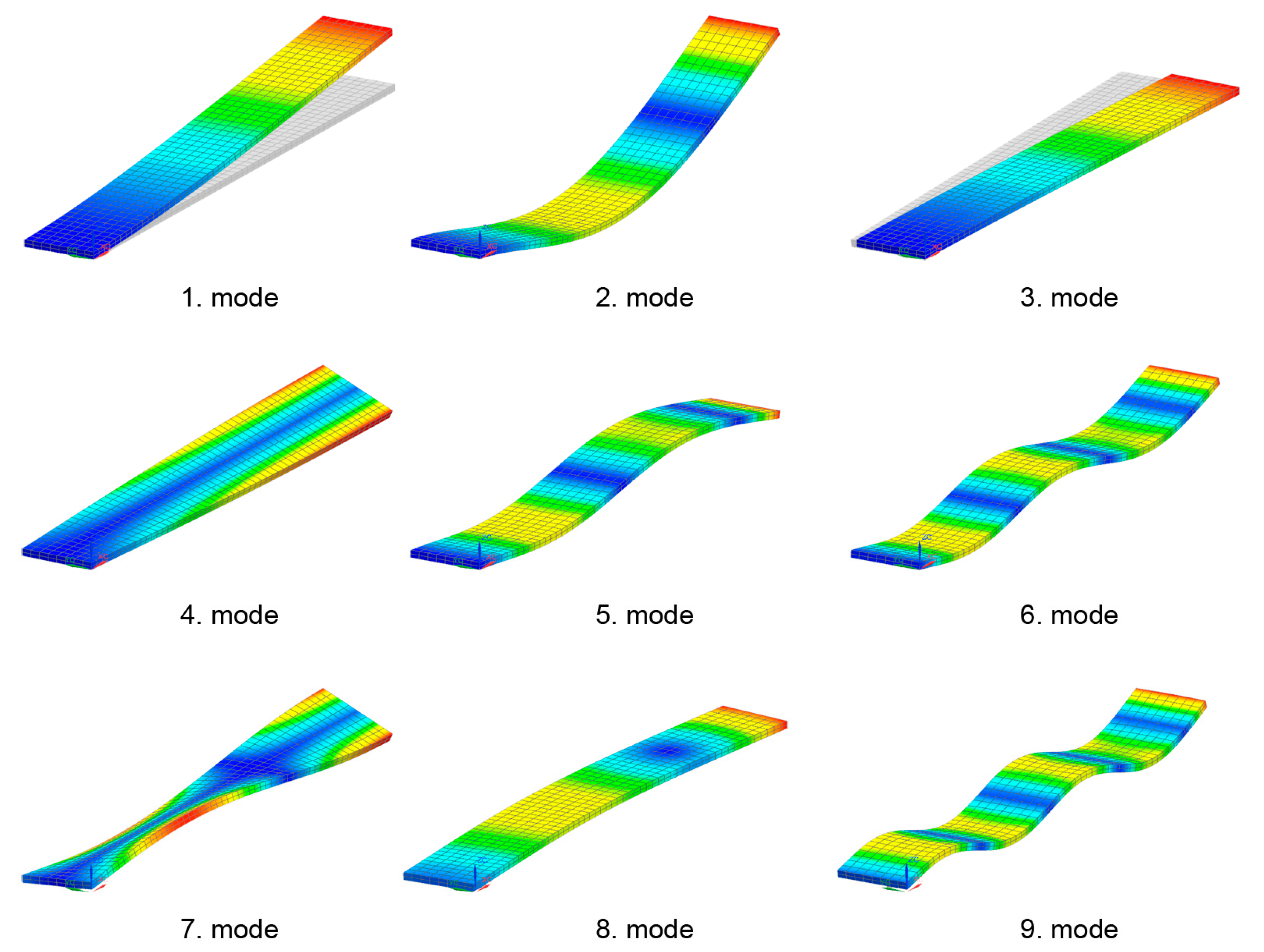
Figure 10.
Mode shapes of the final equivalent FE model.

Figure 11.
Car horn holder and its FE model [32].
Figure 11.
Car horn holder and its FE model [32].

Figure 12.
Bumper FE model.


Table 1.
Material properties of the components.
| Material | Density (kg/m3) | Young Modulus (MPa) | Poisson Ratio (–) |
| Steel | 7850 | 210,000 | 0.3 |
| Aluminum alloy | 2700 | 69,000 | 0.33 |
Table 2.
Bushing stiffness coefficients obtained by FEM.
| The Equivalent Translational Stiffness in x-, y-, z- Direction | ||
 |  |  |
| kx = 3.97 × 10⁵ N/mm | ky = 1.01 × 10⁵ N/mm | kz = 9.8 × 10³ N/mm |
| The Equivalent Rotational Stiffness about x-, y-, z- Axis | ||
 |  |  |
| kφx = 1.547 × 10⁶ N.mm/rad | kφy = 9.72 × 10⁵ N.mm/rad | kφz = 4.5455 × 10⁷ N.mm/rad |
Table 3.
Natural frequencies of compared FE models.
| Mode | Reference Model (Hz) | Equivalent Model (Hz) | Percentage Change (%) |
| 1. | 37.6 | 37.7 | 0.27 |
| 2. | 235.5 | 239.7 | 1.78 |
| 3. | 332.6 | 339.4 | 2.05 |
| 4. | 511.2 | 505.4 | −1.14 |
| 5. | 658.7 | 676.6 | 2.72 |
| 6. | 1289.7 | 1329.7 | 3.10 |
| 7. | 1547.5 | 1533.3 | −0.92 |
| 8. | 1975.4 | 2058.6 | 4.21 |
| 9. | 2129.2 | 2194.7 | 3.08 |
| 10. | 2624.3 | 2610.5 | −0.53 |
| 11. | 3173.7 | 3256.5 | 2.61 |
| 12. | 3765.5 | 3763.1 | −0.06 |
| 13. | 4111.3 | 4107.4 | −0.09 |
| 14. | 4424.3 | 4494.1 | 1.58 |
Table 4.
Modal parameters of the beam obtained by EMA.
| Mode | Damped Frequency (Hz) | Damping Ratio (%) | Mode Shape |
|---|---|---|---|
| 1 | 46.95 | 2.02 | 1. bending |
| 2 | 289.44 | 0.33 | 2. bending |
| 3 | 660.99 | 0.21 | 1. torsion |
| 4 | 810.21 | 0.17 | 3. bending |
| 5 | 1567.15 | 0.08 | 4. bending |
| 6 | 1998.37 | 0.08 | 2. torsion |
| 7 | 2562.31 | 0.27 | 5. bending |
Table 5.
Dimensions and material properties of the equivalent FE model.
| Dimensions (mm) | Density (kg/m3) | Young Modulus (MPa) | Poisson ratio (–) |
| 218 × 30 × 3 | 7850 | 206,000 | 0.3 |
Table 6.
Natural frequencies of the beam obtained by EMA and FEM (Hz).
| Mode | EMA | FEM The Equivalent Model | FEM Clamped-Free Beam Model |
|---|---|---|---|
| 1 | 46.95 | 45.09 (−3.97%) | 52.743 (12.34%) |
| 2 | 289.44 | 291.07 (0.56%) | 330.11 (14.05%) |
| 3 | - | 411.26 | 516.60 |
| 4 | 660.99 | 682.50 (3.25%) | 724.09 (9.55%) |
| 5 | 810.21 | 829.92 (2.43%) | 924.37 (14.09%) |
| 6 | 1567.15 | 1682.42 (7.35%) | 1812.71 (15.67%) |
| 7 | 1998.37 | 2064.50 (3.31%) | 2192.14 (9.69%) |
| 8 | - | 2463.03 | 2992.52 |
| 9 | 2562.31 | 2741.52 (6.99%) | 2998.71 (17.03%) |
The values in parentheses indicate the percentage deviation from the reference values. The frequencies that exceed the tolerance are expressed in red. The frequencies that are within tolerance are marked in green.
Publisher’s Note: MDPI stays neutral with regard to jurisdictional claims in published maps and institutional affiliations. |
© 2021 by the authors. Licensee MDPI, Basel, Switzerland. This article is an open access article distributed under the terms and conditions of the Creative Commons Attribution (CC BY) license (http://creativecommons.org/licenses/by/4.0/).
Share and Cite
MDPI and ACS Style
Huňady, R.; Lengvarský, P.; Pavelka, P.; Kaľavský, A.; Mlotek, J. Stiffness Estimation and Equivalence of Boundary Conditions in FEM Models. Appl. Sci. 2021, 11, 1482. https://doi.org/10.3390/app11041482
AMA Style
Huňady R, Lengvarský P, Pavelka P, Kaľavský A, Mlotek J. Stiffness Estimation and Equivalence of Boundary Conditions in FEM Models. Applied Sciences. 2021; 11(4):1482. https://doi.org/10.3390/app11041482
Chicago/Turabian StyleHuňady, Róbert, Pavol Lengvarský, Peter Pavelka, Adam Kaľavský, and Jakub Mlotek. 2021. "Stiffness Estimation and Equivalence of Boundary Conditions in FEM Models" Applied Sciences 11, no. 4: 1482. https://doi.org/10.3390/app11041482
Note that from the first issue of 2016, this journal uses article numbers instead of page numbers. See further details here.