Ambient Noise Measurements to Constrain the Geological Structure of the Güevéjar Landslide (S Spain)

Abstract

The reactivation of very large landslides may cause severe damage to society. Its prevention and management requires detailed information on the geometry and structure of these landslides, but the use of standard techniques (boreholes) may be prohibitive from an economic point of view. To overcome these difficulties, geophysical techniques are of special interest because they allow for studying very large areas at a reasonable cost. In this paper, we present a case study wherein the analysis of ambient noise allowed us to produce a model of a large landslide near Granada (southern Spain). The geometry and location of the failure zone, as well as the assessment of the state of involved materials, were estimated by combining two available boreholes and different geophysical techniques (downhole tests and the spectral analysis of ambient noise, horizontal to vertical spectral ratios (HVSR) and the frequency-wavenumber (f-k) methods). The results have allowed us to differentiate between values within the landslide mass with respect to those of stable materials, and to perform for the first time a comprehensive geological model of this unstable mass. Differences were also observed within the landslide mass (earth flow vs. slide zones), which are attributed to differences in the degree of alteration and the disturbance of the internal structure of materials constituting the landslide mass. These results show that techniques based on the measurement of ambient noise are of special interest for studying very large, highly remolded landslide masses.

1. Introduction

The occurrence of landslides is a geohazard that affects many places in the world. Landslides may be induced by natural events (rain, earthquakes, volcanoes) and by human activities. When landslides are large, the damage toll may be very high for the society, including casualties [1]. The possible reactivation of such large landslides also represents a severe threat to society [2]. Land-use planning and civil works may mitigate the associated hazard, but for the correct implementation of countermeasures and the management of this kind of hazard, knowing the characteristics of landslides (typology, volume, etc.) is of great interest. Thus, the detailed study of existing large landslides is of prime importance.

Evaluating the possible reactivation of existing large landslides is a complex task. This evaluation requires detailed geological and geomechanical data to assess the stability of a landslide mass in its change when the triggering factors affect the mass. However, this type of study has to face the difficulty of obtaining data for defining the geometry of the landslide mass and characterizing the mechanical and physical properties of the involved materials. The use of traditional in situ methods, such as drilling boreholes and taking undisturbed soil samples, may become economically prohibitive due to their cost, the size of the area to study and the difficulty of drilling in unstable slopes. An economical alternative is needed for the study of very large landslides. For this purpose, the use of geophysical methods is the best solution [3]. Jongmans and Garambois [4] summarized the advantages of these methods for this purpose: (1) these methods are flexible, quick and deployable on slopes, (2) they are not invasive and do not disturb the medium, providing information about the internal structure of the landslide mass, and (3) they allow for investigating large volumes of material in a fast way.

Among the available geophysical techniques, those based on the analysis of seismic noise have become the preferred [3,5]. This is due to their low cost and the type of results they offer (thickness and shear-wave velocity, Vs, of the materials studied), which are useful for defining the inner structure of landslide masses and for studies of their seismic response. The horizontal to vertical spectral ratio (H/V or HVSR) method [6] and different array techniques [7,8,9,10] are the most used procedures for a quick and easy characterization of the soil. The analysis of the HVSR results provides an estimation of the fundamental resonance frequency of the SH waves [11]. The analysis of the array data provides an estimation of the dispersion curve. After that, the resulting curves obtained from the HVSR and array techniques can be inverted in order to estimate the corresponding Vs profile at the site under study. When only one of the HVSR or dispersion curves is available at one site, they can be inverted separately. In other cases when both results are accessible at the same site, a joint inversion of the HVSR and dispersion curves is carried out for the soil characterization [12]. In any case, there is no single solution for the inversion issue. The best solutions can be estimated in terms of a misfit function. Two of the most used inversion methods are the neighborhood [13,14] and the genetic algorithms [15].

The Güevéjar landslide (Granada, southern Spain, Figure 1) is an outstanding example of very large landslide that occurred in the past, likely related to climate conditions different to the present ones. It has had multiple earthquake-induced reactivations, but no activity has been observed due to other triggering factors [16]. The seismic-reactivation history of this landslide started on 1 November 1755, when the Lisbon earthquake (moment magnitude Mw 8.7) struck and reactivated this pre-existing landslide [17]. Because of landslide mass movement, the town of Güevéjar, located on the central part of the landslide mass, was severely damaged [18], but the town was reconstructed when landslide movement stopped. A century later, on 24 December 1884, a Mw 6.5 earthquake struck the provinces of Granada and Málaga in Spain (Figure 1), inducing a new reactivation of this landslide [19]. Historical documents describe that due to the downslope movement of the earth flow existing at the toe of the landslide, a temporary damming of the river existing at the base of the slope occurred [20]. Because of the renewal of movement, the town was so severely damaged that it was finally abandoned. A new town was built approximately 700 m west of its original location, outside of the landslide limits (Figure 2). During the last few decades, old roads and trails have been asphalted, and new houses have been built within the landslide mass.

Despite the size and the seismic history of this landslide, it has been poorly studied. In addition to the studies that describe the reactivation of the landslide during past earthquakes [18], a geological model for this landslide was proposed based on ground surface geological data [21]. In this last study, several landslides existing in the area were grouped into a single one. Based on the proposed model, a study into earthquake-induced reactivation criteria, estimating the magnitude of earthquakes that could reactivate this landslide and the maximum epicentral distance of the occurrence of such events, has been performed [22]. More recently, the mobility of the upper part of this landslide, based on a model created from a limited amount of geophysical data and ground surface geological data, was analyzed through quantitative numerical approaches [23].

In this paper, we perform a comprehensive study of this landslide from a geophysical point of view, with the use of several different seismic techniques based on the measurement of ambient noise. Specifically, single-point measurements and array data are analyzed using the HVSR method and the frequency-wavenumber (f-k) technique [8,24], respectively. Subsequently, the inversion of the HVSR and dispersion curves is carried out by applying the neighborhood algorithm. The results obtained with these methods are constrained by data from boreholes and ground surface geology. The idea is to create the most complete possible model of the considered landslide, useful for later studies about seismic scenarios that could reactivate this landslide in the future. The estimated Vs profiles might be subsequently used for assessing site effects [25].

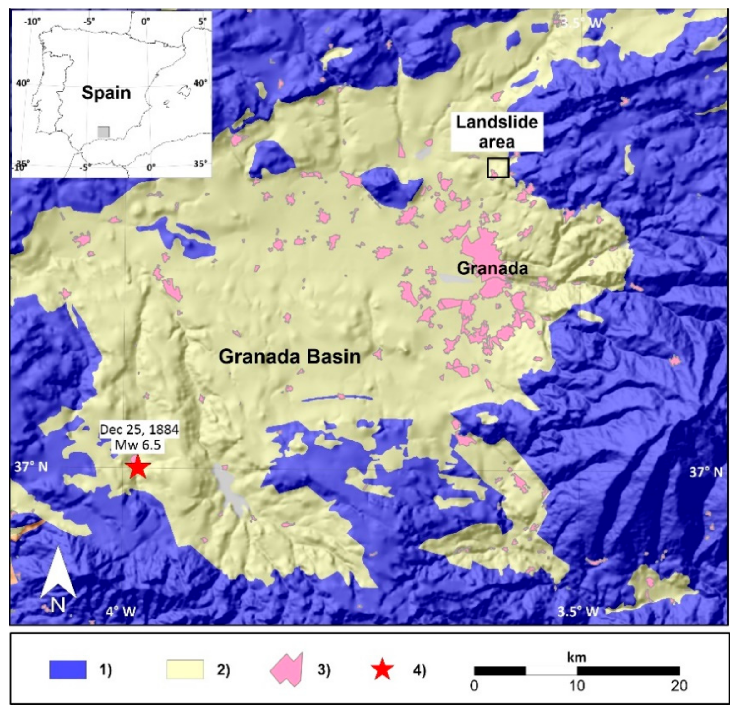
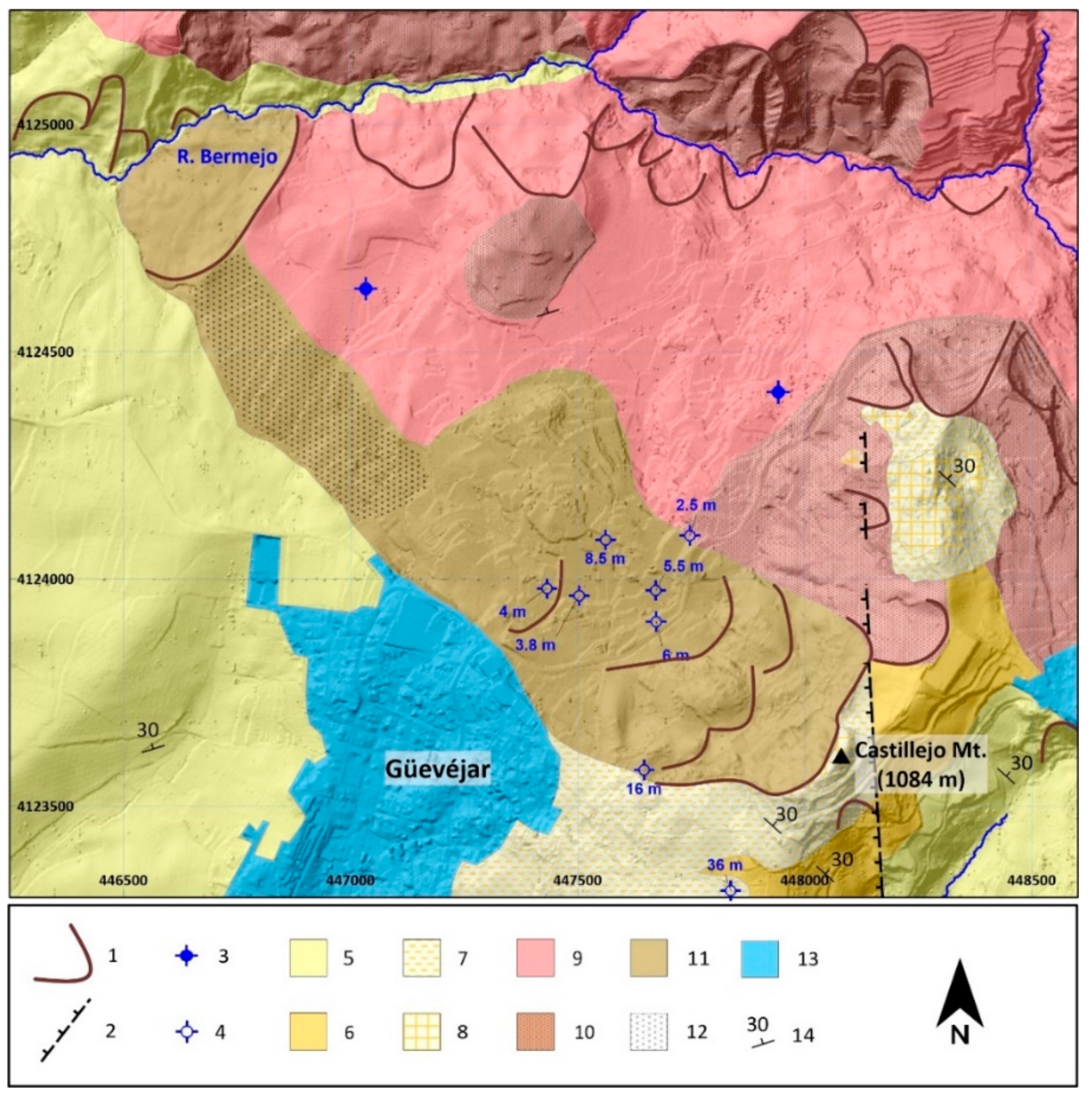
2. Geological Setting

The study zone is located approximately 6 km north of the city of Granada (southern Spain). The landslide affects materials of the sedimentary fill of the Neogene basin of Granada, in the central sector of the Betic Cordillera (Figure 1). This area likely has the highest tectonic activity and seismicity rate in Spain.

The sedimentary record of the basin is up to 2 km in thickness [26]. The basin fill is divided into two different sets: a lower group constituted by marine sedimentary rocks, Upper Miocene in age, and an upper one, of continental sedimentary rocks, Upper Miocene (Turolian) to Quaternary in age [27].

Focusing on the landslide area, all geological formations cropping out in the area belong to the continental group (Figure 2). A first unit consisting of silts, sands and marls (MU unit) is found at the bottom of the stratigraphic series. This unit is more than 100 m thick and shows some transitions between silts, sands and yellowish marls. Marls are more frequent towards the western part of the landslide area, while silts are predominant to the south. This formation contains some thin layers of gypsum and/or limestone. Its age has been identified as late Miocene [28,29]. A second unit consists of red silts, including some layers of clays, sands and highly cemented conglomerates (RSU unit). Both the MU and RSU units are parts of the same depositional environment. The MU unit constitutes the distal deposits of the alluvial fan system developed during the late Miocene in the area, while the RSU unit represents the proximal deposits of this system. Above these units, marls and lacustrine limestone (MLU unit) deposits exist (late Miocene in age). They crop out at the top of Mount Castillejo and in nearby areas (Figure 2). Finally, red clays, sands and conglomerates (recent red deposits, RRD unit) crop out widely north of the landslide area (Pliocene-Pleistocene in age).

This landslide is approximately 2000 m long (from top to toe) with a maximum width of 600 m in its central part. Down the slope, the width of instability decreases and varies between 300 and 400 m near its toe. The landslide may be described as a complex one sensu Cruden and Varnes [30], consisting of a roto-translational earth slide in the upper and middle parts of the slope, and an earth flow downslope (toe of the landslide). The slide affects most of the geological units previously described. At the head of the slide, RSU and MLU units are clearly recognizable in the scarps existing in this area. They show vertical displacement of 2 to 5 m. Several tilted blocks consisting of limestone (MLU unit) resting on red silts (RSU unit) may be found in the upper half of the slide. Due to agricultural activity, the structure of the materials is hardly recognizable in the remaining parts of the landslide. In the lower part, at the base of the slide and in the zone of earth flow, the landslide also involves the RRD unit. In some places, where small ravines have eroded the landslide mass, in situ marls (MU unit) are recognizable.

Historical data of the landslide after the 1884 reactivation describe that large and deep ground cracks were recognizable in the middle part of the landslide, defining large, undisturbed blocks of materials that slid down slope [31]. From the base of the slide body, historical data also describe large debris (earth flow) that flowed downslope, damming the river Bermejo [20].

3. Methodology

3.1. Horizontal to Vertical Spectral Ratios (HVSR) Method

The application of the HVSR technique to ambient vibration signals or seismic noise provides an estimation of the fundamental resonance frequency associated with the site under study. This relation is the fundamental basis of the HVSR analysis [6,32].

Many experiments and theoretical 1D investigations have demonstrated that a strong impedance contrast between the upper layers and the underlying ones (stiffer layers) provides a clear HVSR peak around the fundamental resonance frequency [33,34,35,36,37,38,39]. The HVSR method has become accepted in microzonation studies, since its application and interpretation is straightforward and suitable [40,41,42,43].

The practical implementation of the HVSR method requires only one three-component sensor for the recordings, which makes this technique relatively cheap and easy to implement. In this study, seismic noise measurements were recorded using a broadband seismic station (Guralp CMG-6TD). Approximately 45 min to one hour of seismic noise was captured using a sampling frequency of 100 Hz, recorded in Guralp Compressed Format (GCF). A total of 26 measurements were taken in March 2019, in days of little or no wind in order to avoid disturbances at low frequencies (Figure 3).

The HVSR curves have been estimated using the GEOPSY software from the Sesarray package [44]. The recorded signals have passed through an anti-triggering filter, and then they have been divided into non-overlapping windows of frequency-dependent length. Each window was tapered by a 5% cosine function and its length was 50 periods of the frequency analyzed at each moment [45]. After that, the frequency response was obtained for each window and component, and smoothed applying a Konno and Omachi window (coefficient b = 40) [46]. Subsequently, for each window, the squared average of the horizontal components was computed and then the horizontal-to-vertical spectral ratio was calculated. Finally, the HVSR curves from the selected windows have been averaged to provide the mean HVSR curve and its corresponding standard deviation.

3.2. Downhole Measurements

Geotechnical exploration was carried out in September 2014 to develop a first approximation of the soil characteristics. More specifically, two boreholes were drilled along the main direction of the landslide (Figure 3) just where the historical town was located, to the northeast of the present Güevéjar town. The maximum depths were 60 (borehole S2, Figure 4) and 70 m (S1, Figure 4), respectively.

The tests were performed by Geytex SL company. They operated an exploration seismograph (model GEODE 12, 24 bits, Geometrics, San Jose, CA, USA) with triaxial geophones and a heavy hammer as the seismic source. The hammer hits a steel rod that had been previously fixed to the ground surface. Measurements were taken every meter along the borehole until reaching its base.

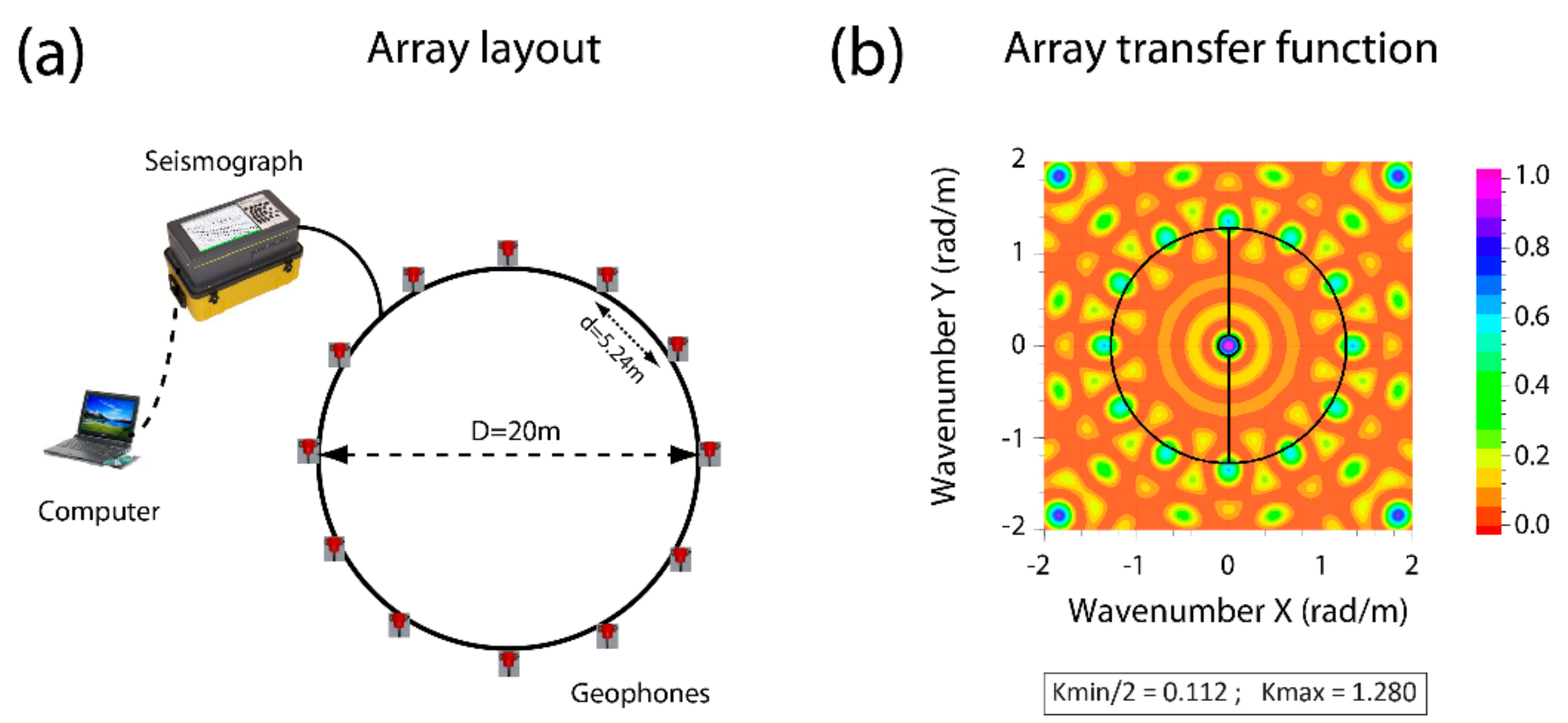
3.3. Frequency-Wavenumber (f-k) Analysis

The f-k method is an array technique based on the analysis of seismic noise. Assuming stationary noise in both time and space, the incoming waves can be represented as a function of the frequency and the vector velocities through the frequency-wavenumber spectral density function [8,24]. Thus, the wave velocities and their respective directions of approach are derived as functions of the frequency.

The power spectrum can be obtained through the maximum likelihood method (MLM) [8] or the beam-forming method (BFM) [24], which is the one used in this work. Additional information can be found elsewhere [47,48,49].

The seismic noise array measurements were taken around the Güevéjar landslide at eight different sites (Figure 3). The implementation of the arrays was achieved with seismic refraction/reflection equipment consisting of twelve 4.5 Hz vertical geophones connected to a multichannel seismic recorder (SmartSeis ST, Geometrics, San Jose, CA, USA). A circular layout without a central station was deployed for the array layout (Figure 5a). For all the sites, the diameter of the arrays was configured to 20 m, which is the maximum possible aperture allowed by the cable length of the reflection/refraction equipment used. Taking into account that the wavelengths obtained by the f-k method can be several times greater than the array diameter [50,51], this configuration would be enough for the soil classification purposes [52].

The data acquisition consisted of approximately fifty records of 32 s without overlapping, sampled at 500 Hz and subsequently resampled at 100 Hz. Although the natural frequency of the geophones is 4.5 Hz, this equipment allows for estimating dispersion curves above approximately 2 Hz [53,54].

In Figure 5b, we show the theoretical response of the array, providing estimates of the aliasing (kmax) and the maximum resolution (kmin/2) limits, in terms of the wavenumber.

The f-k analysis has also been accomplished using the GEOPSY software. The initial configuration requires the establishing of the grid of wavenumber (k) points to be analyzed, indicating the maximum value (grid size) as well as the minimum step (grid step). These values determine the aliasing limit and the maximum resolution, respectively. For the arrangement carried out in this work, the analysis of the theoretical array response provides a maximum resolution of 0.06 rad/m (kmin/4) and an aliasing limit of 0.64 rad/m (kmax/2) (see Figure 5b). The real array response depends on the number of sensors and the sensor geometry, but also on the slowness and the wavenumbers of the seismic phases observed within the array.

With these considerations, a dispersion curve is first estimated for each analyzed 32 s window, which corresponds with the length of the recordings. Finally, a mean dispersion curve is computed by averaging the curves obtained from all the windows.

3.4. Inversion of the Dispersion and HVSR Curves

The HVSR and dispersion curves are inverted using the neighborhood algorithm to obtain an optimal estimation of the Vs profiles [14]. The inversion process explores a defined parameter space (number of layers, S-wave velocity, P-wave velocity, density and layer thickness) in search of possible solutions. The results previously obtained from borehole drills and downhole experiments have helped to constrain the number of layers and their corresponding thickness and S-wave velocity ranges. Poisson’s ratio and density values have been set up for all the layers in the range of 0.2–0.5 and 1600–2200 kg/m³, respectively, which correspond to the characteristics of the materials in the studied landslide.

The ellipticity of the fundamental mode Rayleigh wave or the dispersion curve is estimated for each computed model (forward problem), and then contrasted with the empirical curves using a misfit function [55], which reflects quantitatively the difference between the generated models and the observed results.

For the calculation of the Vs profiles, the Dinver software from the Sesarray package has been used [44]. This software allows the inversion of dispersion and ellipticity curves. In the case of the dispersion curves, they are obtained directly from the f-k analysis. In the case of the ellipticty curves, they were previously extracted from the experimental HVSR curves [42,56] and then used as input data of the Dinver software. Alternatively, HVSR curves can also be used as input data if some considerations are taken into account [41,57]. For large velocity contrast, Fäh et al. [58,59] showed that HVSR curves are dominated by the ellipticity of the fundamental mode Rayleigh wave in the frequency band between the fundamental resonant frequency and the next minimum, with its shape being dominated by the specific layering of the sediments. With regards to these indications, in this work the frequency band around the main resonant peak has been considered for the inversion process. Only in the cases where a secondary peak or hump has also been identified have we broadened the frequency interval to include also this peak, as this could provide information about other velocity contrasts or interfaces.

4. Results and Discussion

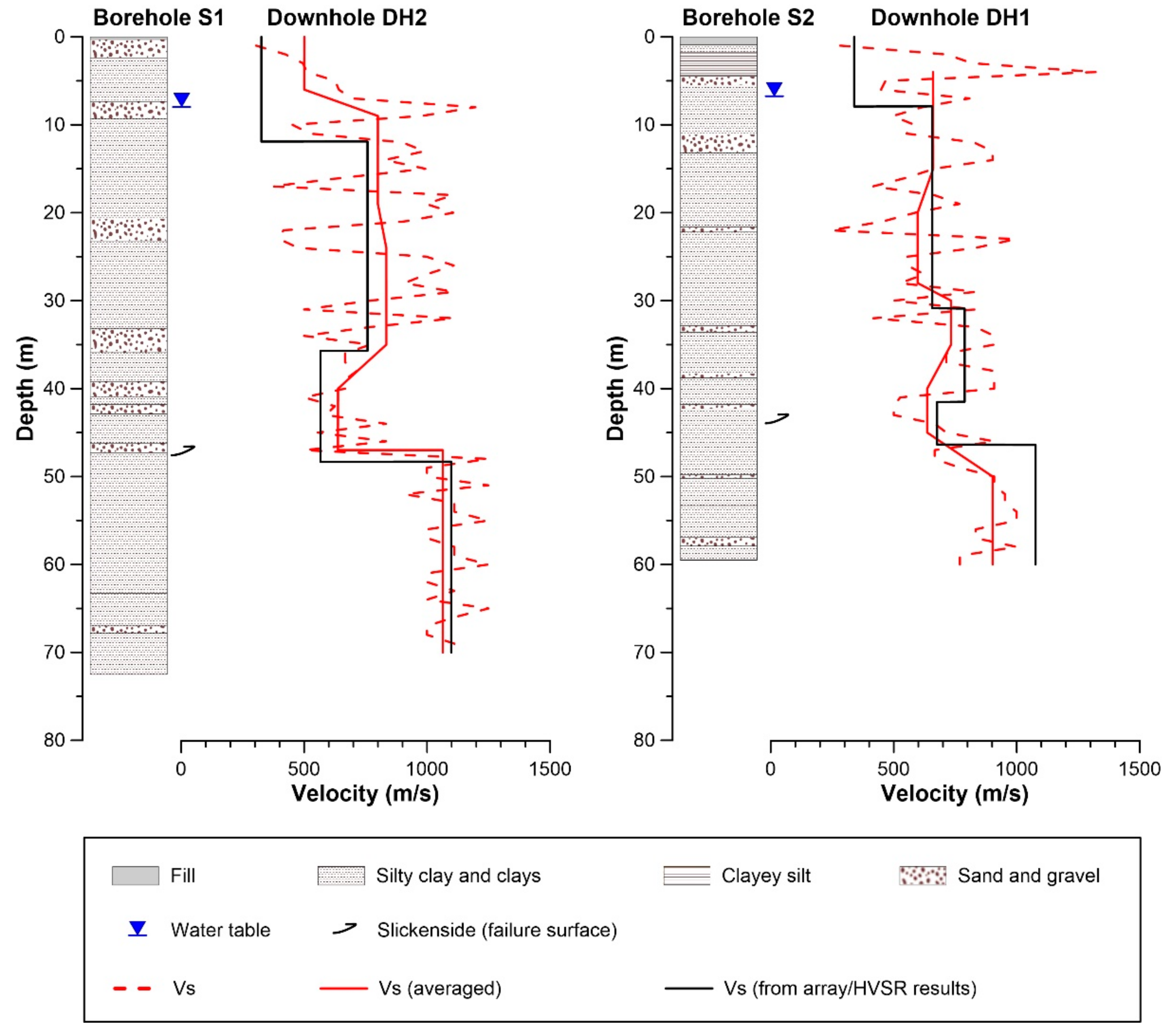
4.1. Downhole Results

We have used the information provided from two boreholes drilled in the area (Figure 3) to identify the main characteristics of the soil columns. In Figure 4, the stratigraphic information from the boreholes and the Vs profiles deduced from the downhole test are depicted. The soil columns observed at both boreholes show a series of reddish silty clay and clayey silt levels with thin sand or conglomerate levels. At depths of 43 m (at borehole S2) and 48 m (S1), the soil samples showed polished surfaces, which are interpreted as slickensides formed by the slip along a failure surface of the landslide. The water table is found at less than 10 m in both boreholes.

The first borehole (S1) was drilled to a depth of 70 m (Figure 4). From the downhole study, we deduced a three-layer Vs profile. The first layer has a thickness of 5–10 m and a Vs value less than 500 m/s. The second layer reaches a depth of 40–43 m with a Vs value of approximately 800–900 m/s. Finally, the depth of the third layer is between 43 and 50 m with a Vs of 600–700 m/s. Below 43–50 m, hard materials are found with a Vs value of approximately 1000 m/s.

The second borehole (S2) was drilled to a depth of 60 m (Figure 4). From the downhole study, we deduced a four-layer Vs profile. The first layer of fills and clayey silts presents a maximum thickness of 5 m and a Vs value less than 500 m/s, which is similar to that observed at S1. The depth of the second layer lies between 25 and 30 m with an average Vs value of approximately 700 m/s. The third layer reaches a depth of 35–40 m and presents a Vs value of 800–900 m/s. Finally, the depth of the fourth layer is found at approximately 45–50 m, with a Vs value of approximately 700 m/s. Below 45–50 m, hard materials are found, presenting a Vs value close to 1000 m/s.

The deeper layers on both profiles are located below the surface failures identified in the soil columns, and represent the in situ materials. They show a certain contrast in the measured velocities with respect to shallower layers (Figure 4). Sudden increases in Vs velocities in S1 just below the failure surface are evident. In S2, this contrast is not as clear, but even in this case, it is recognizable that the Vs is lower at the zone of failure than the values observed in materials above and below this zone.

4.2. HVSR Analysis Resonance Frequencies

In Figure 6, some representative cases of the HVSR curves obtained along the landslide are shown. The locations of some of these sites, close to the landslide flanks, may explain the presence of some broad peaks with rather low amplitudes. At these sites, the wavefields associated with local noise sources are more complex, since the wavefields also include additional waves diffracted from the lateral heterogeneities. Experimental tests and numerical simulations have shown that, for local surface sources, the HVSR curves obtained at laterally varying structures present broader and lower maxima, which may even be hard to identify [60].

In our study case, the resonance frequency, f, associated with the contrast between the sediments and the stiffer materials below the landslide, can be related to the average shear-wave velocity of this one-dimensional stratigraphy, Vs, and the corresponding thickness, h, through the equation [33]:

f (Hz) = Vs/(4 h)

(1)

Therefore, attending to the borehole information, it can be estimated that the resonance frequencies of interest for the landslide characterization present values higher than 2 Hz. In this case, peaks below 2 Hz might be associated with deeper contrasts from the contacts between materials of the sedimentary fill of the Granada basin (or between this fill and the basement).

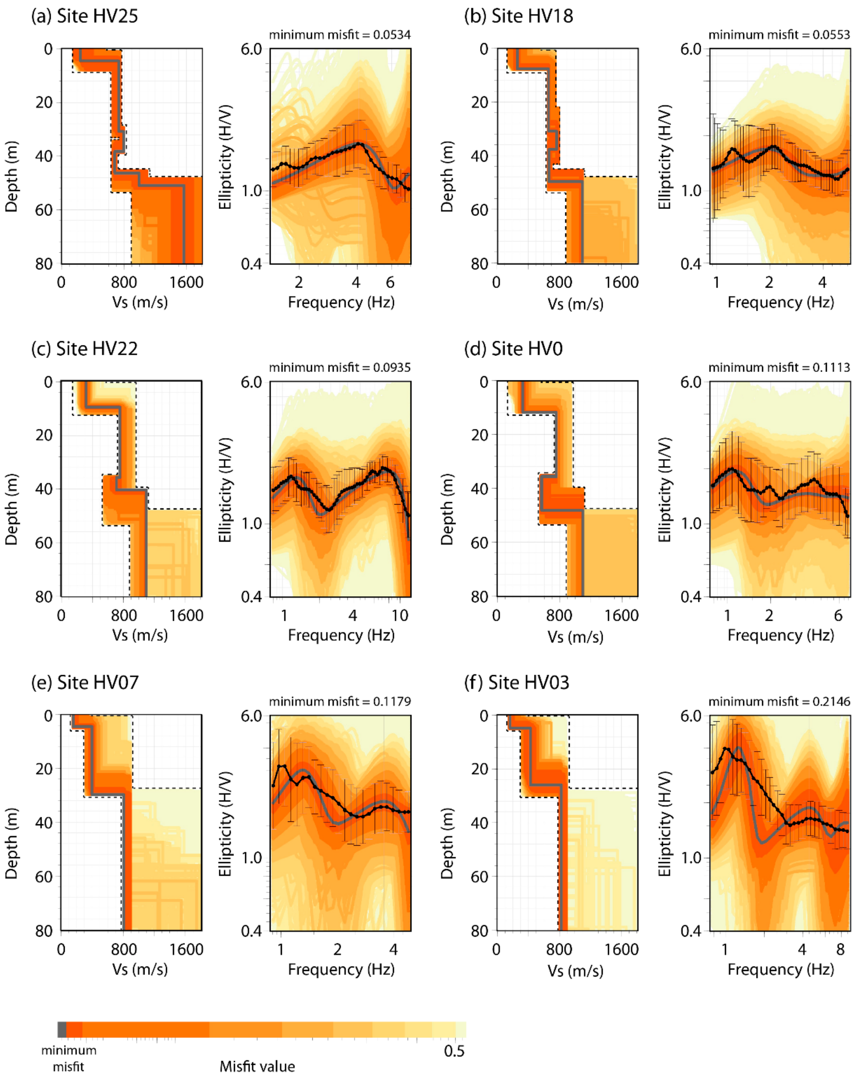
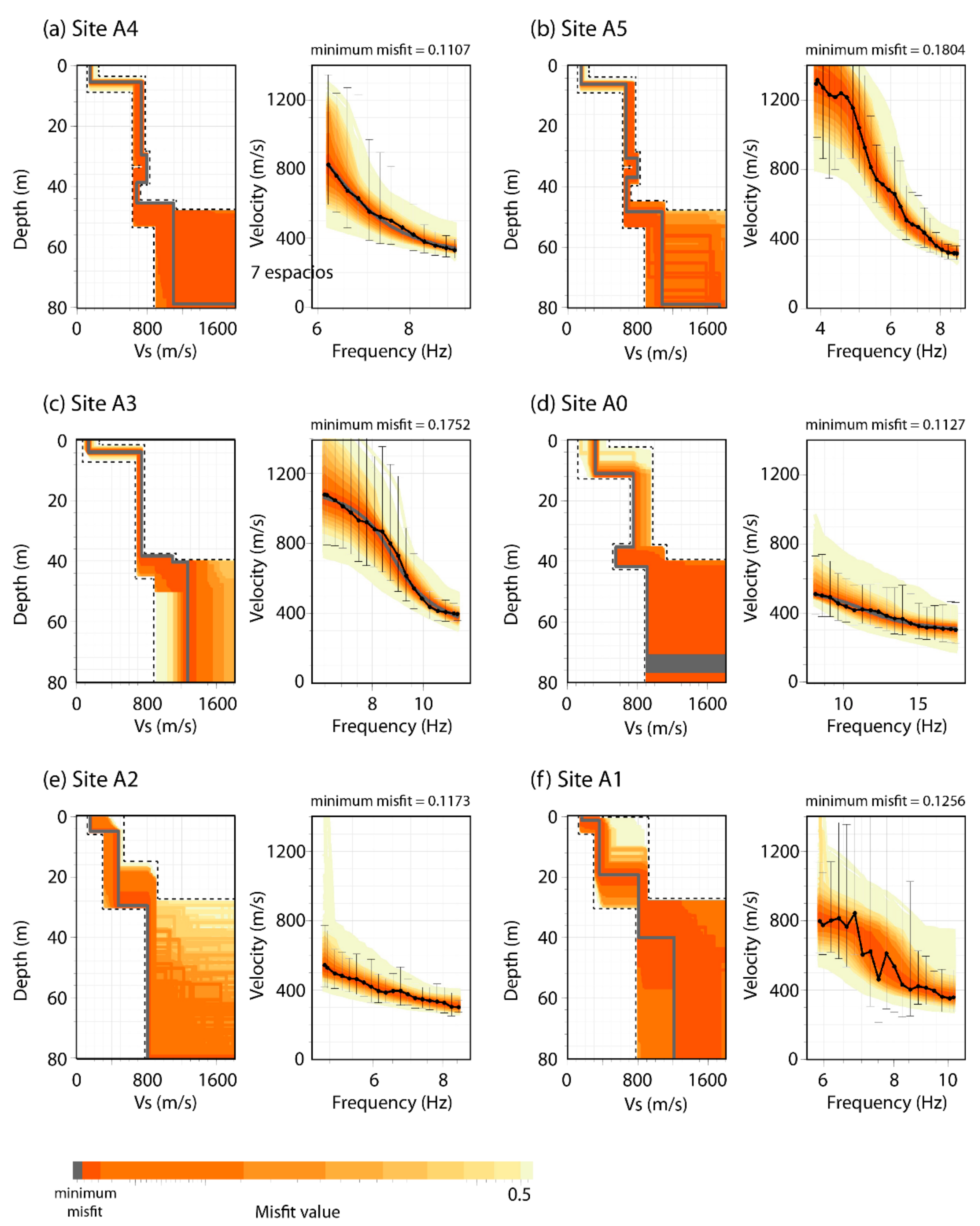
4.3. S-Wave Velocity Profiles

HVSR and dispersion curves have been inverted separately, as they were obtained at different sites within the landslide. The number and the thickness of layers, as well as the range of Vs values obtained from the downhole results (see Section 4.1), have been used to constrain the parameter space in the sites around the central area of the landslide. In the case of the thickness and Vs values, an additional margin around the value ranges deduced from the boreholes has been included because the measurement points do not match exactly at the borehole sites (see Figure 3). For the sites closest to the first borehole (S1), the following model has been used: a first layer with maximum thickness of 12 m and shear-wave velocity between 150 and 550 m/s; a second layer that reaches a maximum depth between 35 and 43 m and has a Vs value between 750 and 950 m/s; and a third layer whose maximum depth reaches 45–53 m, with a Vs value of 550–750 m/s. Below this, a hard layer is configured with a minimum depth of 48 m and velocities between 900 and 1100 m/s.

In the cases of the sites closest to the second borehole (S2), a four-layer model has been applied with the following characteristics: a first layer with maximum thickness of 8 m and shear-wave velocity between 150 and 550 m/s; a second layer whose maximum depth reaches 22–33 m, with Vs value of 650–750 m/s; a third layer with maximum depth and shear-wave velocity in the ranges 33–43 m. and 750–800 m/s, respectively; and a fourth layer that reaches a limit depth of 45–53 m., and a Vs of 650–700 m/s. Below, a hard layer is configured with a minimum depth of 48 m and velocities between 900 and 1000 m/s.

In all cases, an additional harder layer has been added to these models in order to take into account possible deeper velocity contrasts. The profiles obtained at these two sites are shown in Figure 4, showing a remarkable similarity with the results of the downhole tests.

For those sites closer to the expected border of the landslide, a simpler model has been used with two sedimentary layers over two harder layers, representing the in situ stable materials. The superficial layer is included to take into account the shallower materials, disturbed by agricultural activities. The inclusion of two harder layers allows also for adjusting the estimated model to the HVSR peaks found below 2 Hz, which might be associated with deeper contrasts.

The fitting carried out by the software is based on a multimode surface-wave modeling through a vertically heterogeneous, elastic and isotropic medium. The model generation process implies the computation of the theoretical ellipticity, or dispersion curves, of the fundamental mode Rayleigh wave (forward model), and a comparison with the respective experimental curves. The similarity between the theoretical and the empirical HVSR or dispersion curves is expressed quantitatively by a misfit value.

Figure 7 and Figure 8 depict some examples of the Vs profiles estimated using the HVSR curves, and the dispersion curves obtained by the f-k method, respectively. From the estimated profiles, we can observe how the obtained results with both techniques are coherent with each other.

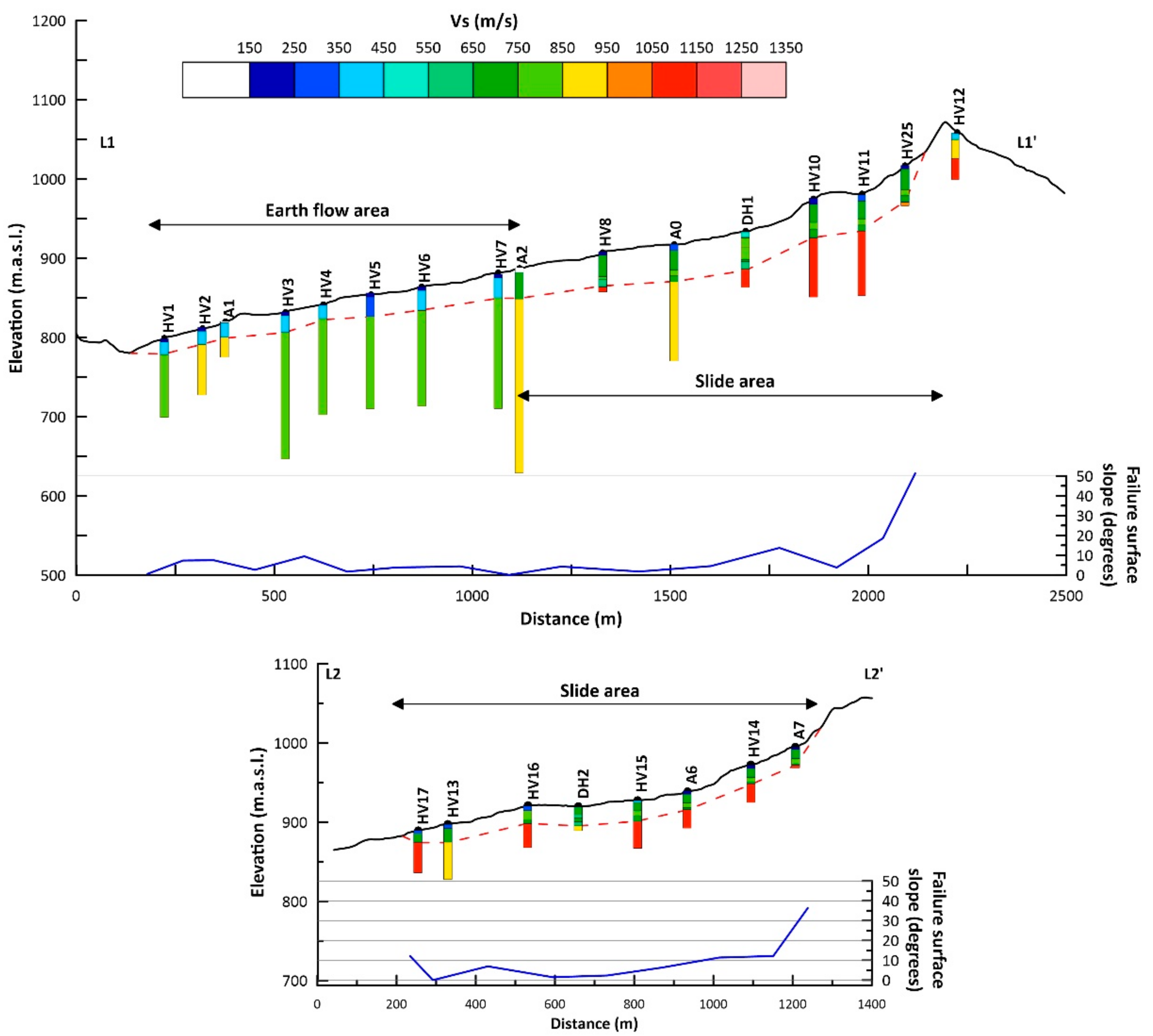
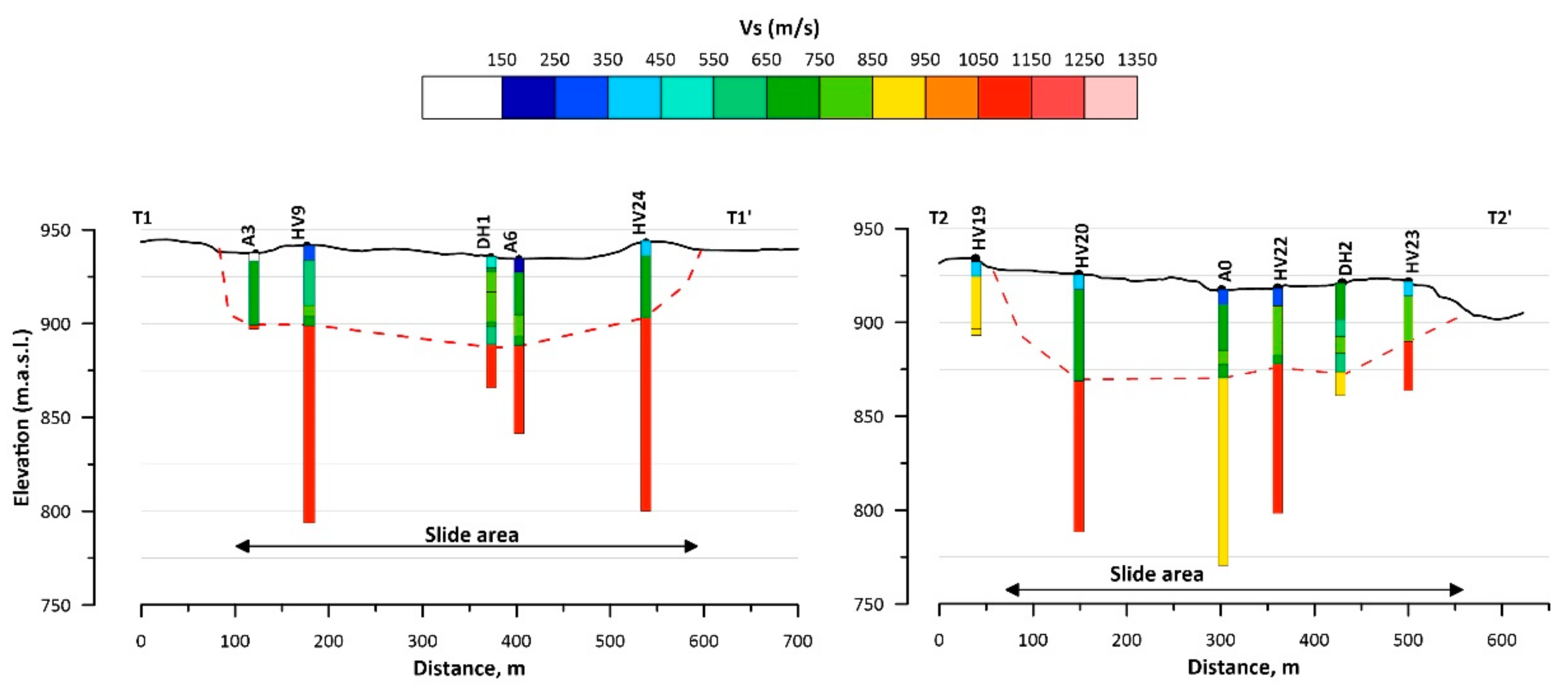
4.4. Landslide Geological Structure

The results obtained from the geophysical studies on the Güevéjar landslide are integrated and synthesized with ground surface geology in order to build, for the first time, a model of the whole unstable mass (Figure 9 and Figure 10). The landslide limits are based on data from boreholes and on the contrast in shear wave velocities found with depth. Superficial limits are based on field observations and on observations supplied by land owners.

The results show that the whole area is characterized by a shallow layer with very low Vs velocity (average value of 251 m/s, ranging from 139 to 422 m/s). Its thickness varies irregularly (6.6 m on average, ranging from 1.1 up to 11.9 m), although the greater values are found in the central part of the slide area (thickness > 5 m), where a gentle slope exists (Figure 9 and Figure 10). The obtained values are in agreement with those observed in the available borehole soil columns. This layer is found elsewhere, in both landslide and stable terrain areas. It is interpreted as a shallow layer of alteration due to several not exclusive possible causes (weathering, agricultural activities, fills or the deposition of debris in low areas).

In the landslide area, below the shallow layer, a second layer exists exhibiting a complex pattern of velocities, depending on whether it is found in the earth flow or in the slide deposits. At the lower parts of the slope, corresponding with the area where the earth flow is, a layer with moderate Vs exists, averaging 375 m/s (ranging from 340 to 427 m/s), with thicknesses varying in the range of 16–25 m (Figure 9). Such thicknesses reduce towards the flanks of the instability, as is seen in some ravines that have partially eroded landslide mass. The observed Vs velocities may be related to the degree of disturbance of the materials involved in the landslide. The materials involved in the earth flow are characterized by a high degree of disturbance, and they are altered to a soil state. A significant reduction in Vs is expected with respect to the same undisturbed materials.

In the zone occupied by slide deposits, this second layer may comprise several sublayers. Downhole tests show moderate Vs values (500–800 m/s; Figure 4) for these sublayers. Similar results are obtained at most of the sites where HVSR (Figure 7) or arrays (Figure 8) measurements were accomplished. The average Vs value of all sublayers is 710 m/s, markedly higher than the Vs of earth flow deposits. This may be explained by the lower degree of disturbance of the materials involved. Between all measurement sites, the sum of the thicknesses of all sublayers varies from 24 m up to 48 m (Figure 9 and Figure 10).

The lower limit of landslide, or failure surface, is attributed to a sudden increase in Vs with depth observed below the layer previously described, in accordance with results observed in the boreholes drilled and downhole tests. Below the earth flow area, Vs > 800 m/s, resulting in a high contrast with earth flow deposits (average increase in Vs > 100%). The resulting surface shows a gentle dip towards the base of the slope (Figure 9). Below the slide area, materials show an average Vs of 1060 m/s (ranging from 910 to 1100 m/s; average increase > 50%), and the failure surface is more irregular than in the earth flow area (Figure 9 and Figure 10), with changes in relation to the secondary failures recognizable in the field (Figure 2). It is interesting to note that, for the in situ materials, lower values of Vs coincide with the spatial distribution of marls of the MU unit, while higher Vs values were found in areas where RSU and MLU materials crop out (Figure 3, Figure 9 and Figure 10).

The resulting model of the landslide shows that its maximum thickness is approximately 56 m in the western part (site HV20; Figure 3 and Figure 10). This value results from the sum of thicknesses of surficial layer and that below it. This thickness decreases slowly to 45–50 m towards the crown area of the landslide (sites A5, HV10, HV14 and HV18). The thickness of earth flow ranges between 20 and 30 m at the center of the lobe, where the measurements were performed. Towards the flanks, thickness decreases progressively. The reconstructed geometry is consistent with the results obtained from the numerical modeling performed in previous studies [23], which justifies the main local resonance as related to the landslide thickness, while landslide mobility seems to be more strictly linked to its longitudinal dimension (length). This justifies the unexpected reactivation of the Güevéjar landslide in the past, such as when it was triggered by the 1755 Lisbon earthquake.

5. Conclusions

The high-resolution engineering–geological modeling and characterization of large landslides is complex when the application of standard geotechnical techniques is unfeasible. This is mainly due to the large number of required investigations and the difficulty of drilling in unstable slopes. As an alternative, seismic methods based on ambient noise measurements are used to characterize the geometry and the underground distribution of materials. Specifically, HVSR and array measurements (f-k analysis) have been combined properly along the studied landslide area. In such a large and complex geological structure, the data analysis is carried out from the central area of the landslide towards its lateral limits. In addition, geotechnical information, when available, has to be used to constrain the range of the expected Vs models estimated from the inversion of HVSR and/or dispersion curves. The combination of different techniques provides more robustness to the estimated Vs profiles.

Therefore, the results obtained here from the use of ambient noise and their interpretation with several geophysical techniques are useful for building a comprehensive model for the Güevéjar landslide based on the contrast in velocities between in situ materials and the landslide mass. This model allows for distinguishing two zones characterized by different landslide mechanisms: the first one, located at the upper slope, is related to a sliding slope failure, and the second one, located on the downslope, is related to an earth flow. It is also possible to highlight differences in Vs values within the landslide mass: minimum Vs values are found in the earth flow that exists at the toe of the landslide (average Vs = 375 m/s), while higher Vs values appear in the middle and upper parts of the landslide (average Vs = 710 m/s). These changes may be interpreted as a function of the degree of disturbance/alteration of the geological materials involved in the landslide: the earth flow implies the total loss of the internal structure of the materials, whereas the slide dislodges the materials into blocks that move as a whole, preserving most of their internal structure.

These results show the usefulness of the set of geophysical methods implemented in this study, based on the measurement and inversion of ambient noise data, for analyzing very large landslides at a reasonable cost. The relation between the degree of material damage and the resulting Vs values makes these techniques of special interest for studying multiple landslide mechanisms, such as sliding, or disorganized ones, such as flows.

References

1. Sassa, K. The ISDR-ICL Sendai Partnerships 2015–2025: Background and content. In Advance Culture of Living with Landslides, ISDR-ICL Sendai Pertnerships 2015–2025; Sassa, K., Mikos, M., Yin, Y., Eds.; Springer: Berlin/Heidelberg, Germany, 2017; Volume 1, pp. 3–21. [Google Scholar] [CrossRef] [Green Version]
2. Lari, S.; Frattini, P.; Crosta, G.B. A probabilistic approach for landslide hazard analysis. Eng. Geol. 2014, 182, 3–14. [Google Scholar] [CrossRef] [Green Version]
3. Pazzi, V.; Morelli, S.; Fanti, R. A review of the advantages and limitations of geophysical investigations in landslide studies. Int. J. Geophys. 2019, 27, 2983087. [Google Scholar] [CrossRef] [Green Version]
4. Jongmans, D.; Garambois, S. Geophysical investigation of landslides: A review. Bull. Soc. Géol. France 2007, 178, 101–112. [Google Scholar] [CrossRef] [Green Version]
5. D’Amico, S.; Panzera, F.; Martino, S.; Iannucci, R.; Paciello, A.; Lombardo, G.; Galea, P.; Farrugia, D. Chapter 12-Ambient noise techniques to study near-surface in particular geological conditions: A brief review. In Innovation in Near-Surface Geophysics; Persico, R., Piro, S., Linford, N., Eds.; Elsevier: Amsterdam, The Netherlands, 2019; pp. 419–460. [Google Scholar] [CrossRef]
6. Nakamura, Y. A method for dynamic characteristics estimation of subsurface using microtremors on the ground surface. Quart. Rep. Railw. Tech. Res. Inst. Jpn. 1989, 30, 25–33. [Google Scholar]
7. Aki, K. Space and time spectra of stationary stochastic waves, with special reference to microtremors. Bull. Earthq. Res. Inst. Tokyo Univ. 1957, 25, 415–457. [Google Scholar]
8. Capon, J. High-resolution frequency-wavenumber spectral analysis. Proc. IEEE 1969, 57, 1408–1419. [Google Scholar] [CrossRef] [Green Version]
9. Ling, S.; Okada, H. An extended use of the spatial autocorrelation method for the estimation of geological structure using microtremors. In Proceedings of the 89th SEGJ Conference, Nagoya, Japan, 12–14 October 1993; pp. 44–48. [Google Scholar]
10. Park, C.B.; Miller, R.D.; Xia, J.; Ivanov, J. Multichannel analysis of surface waves (MASW)-active and passive methods. Lead. Edge 2007, 26, 60–64. [Google Scholar] [CrossRef]
11. Bonnefoy-Claudet, S.; Cornou, C.; Bard, P.Y.; Cotton, F.; Moczo, P.; Kristek, J.; Fah, D. H/V ratio: A tool for site evaluation. Results from 1–D noise simulations. Geophys. J. Int. 2006, 67, 827–837. [Google Scholar] [CrossRef] [Green Version]
12. Picozzi, M.; Parolai, S.; Richwalski, S.M. Joint inversion of H/V ratios and dispersion curves from seismic noise: Estimating the S-wave velocity of bedrock. Geophys. Res. Lett. 2005, 32, L11308. [Google Scholar] [CrossRef]
13. Sambridge, M. Geophysical inversion with a neighbourhood algorithm I. Searching a parameter space. Geophys. J. Int. 1999, 138, 479–494. [Google Scholar] [CrossRef] [Green Version]
14. Wathelet, M. An improved neighborhood algorithm: Parameter conditions and dynamic scaling. Geophys. Res. Lett. 2008, 35. [Google Scholar] [CrossRef] [Green Version]
15. Yamanaka, H.; Ishida, H. Application of genetic algorithms to an inversion of surface wave dispersion data. Bull. Seismol. Soc. Am. 1996, 86, 436–444. [Google Scholar]
16. Delgado, J.; Peláez, J.A.; Tomás, R.; García-Tortosa, F.J.; Alfaro, P.; López Casado, C. Seismically-induced landslides in the Betic Cordillera (S Spain). Soil Dyn. Earthq. Eng. 2011, 31, 1203–1211. [Google Scholar] [CrossRef]
17. Martínez Solares, J.M.; López Arroyo, A. The great historical 1755 earthquake. Effects and damage in Spain. J. Seismol. 2004, 8, 275–294. [Google Scholar] [CrossRef]
18. Sanz, E. Le mouvement de versant de Güevejar (Grenade) au cours des tremblements de terre de Lisbonne (1755) et d’Andalousie (1884). Bull. Interintl. Assoc. Eng. Geol. 1997, 56, 83–87. [Google Scholar]
19. Instituto Geográfico Nacional. El Terremoto de Andalucía del 25 de Diciembre de 1884; Publicaciones IGN: Madrid, Spain, 1980; 139p. [Google Scholar]
20. Fernández Castro, M.; Lasala, J.P.; Cortázar, D.; Gonzalo Tarín, J. Terremoto de Andalucía: Informe de la Comisión nombrada para su estudio dando cuenta del estado de los trabajos en 7 de marzo de 1985. Boll. Com. Mapa Geol. Esp. 1885, 12, 1–105. [Google Scholar]
21. Jiménez-Pintor, J.; Azor, A. El Deslizamiento de Güevéjar (provincia de Granada): Un caso de inestabilidad de laderas inducida por sismos. Geogaceta 2006, 40, 287–290. [Google Scholar]
22. Rodríguez-Peces, M.J.; García-Mayordomo, J.; Azañón, J.M.; Insúa, J.M.; Jiménez Pintor, J. Constraining pre-instrumental earthquake parameters from slope stability back-analysis: Palaeoseismic reconstruction of the Güevéjar landslide during the 1st November 1755 Lisbon and 25th December 1884 Arenas del Rey earthquakes. Q. Intern. 2011, 242, 76–89. [Google Scholar] [CrossRef]
23. Martino, S.; Lenti, L.; Delgado, J.; Garrido, J.; López-Casado, C. Application of a Characteristic Periods-Based (CPB) approach to estimate earthquake-induced displacements of landslides through dynamic numerical modelling. Geophys. J. Int. 2016, 206, 85–102. [Google Scholar] [CrossRef] [Green Version]
24. Lacoss, R.T.; Kelly, E.J.; Toksöz, M.N. Estimation of seismic noise structure using array. Geophysics 1969, 29, 21–38. [Google Scholar] [CrossRef]
25. Ohrnberger, M.; Scherbaum, F.; Krüger, F.; Pelzing, R.; Reamer, S.K. How good are shear wave velocity models obtained from inversion of ambient vibrations in the lower Rhine embayment (N.W. Germany). Boll. Geofis. Teor. Appl. 2004, 45, 215–232. [Google Scholar]
26. Rodríguez-Fernández, J.; Sanz de Galdeano, C. Late orogenic intramontane basin development: The Granada basin, Betics (Southern Spain). Basin Res. 2006, 18, 85–102. [Google Scholar] [CrossRef] [Green Version]
27. Fernández, J.; Soria, J.M.; Viseras, C. Stratigraphic architecture of the Neogene basins in the central sector of the Betic Cordillera (Spain): Tectonic control and base level changes. In Tertiary Basins of Spain: The Stratigraphic Record of Crustal Kinematics; Friend, P.F., Dabrio, C.J., Eds.; Cambridge University Press: Cambridge, UK, 1996; pp. 353–365. [Google Scholar]
28. Dabrio, C.J.; Fernández, J.; Peña, J.A.; Ruiz-Bustos, A.; Sanz de Galdeano, C. Rasgos sedimentarios de los conglomerados miocenos del borde Noreste de la Depresión de Granada. Estud. Geol. 1978, 343, 89–97. [Google Scholar]
29. Dabrio, C.J.; Fernández, J.; Peña, J.A.; Ruiz-Bustos, A.; Sanz de Galdeano, C. Interpretation sedimentaire des materiaux néogènes du bord nord-est du Bassin Grenade (Espagne). C.R. Somm. Seanc. Soc. Geol. France 1978, 3, 121–123. [Google Scholar]
30. Cruden, D.M.; Varnes, D.J. Landslide type and processes. In Landslides. Investigation and Mitigation; Special Report 247; Turner, A.K., Schuster, R.L., Eds.; Transportation Research Board, National Academy Press: Washington, DC, USA, 1996; pp. 36–75. [Google Scholar]
31. Meléndez, B.; Fuster, J.M. Geología; Paraninfo: Madrid, Spain, 1966; p. 687. [Google Scholar]
32. Nogoshi, M.; Igarashi, T. On the propagation characteristics estimations of subsurface using microtremors on the ground surface. J. Seism. Soc. Japan 1971, 23, 264–280. [Google Scholar]
33. Lermo, J.; Chávez-García, F.J. Site effect evolution using spectral ratios with only one station. Bull. Seismol. Soc. Am. 1993, 83, 1574–1594. [Google Scholar]
34. Lachet, C.; Bard, P.Y. Numerical and theoretical investigations on the possibilities and limitations of the Nakamura’s technique. J. Phys. Earth. 1994, 42, 377–397. [Google Scholar] [CrossRef]
35. Field, E.H.; Jacob, K.H. A comparison and test of various site response estimation techniques, including three that are non reference–site dependent. Bull. Seismol. Soc. Am. 1995, 85, 1127–1143. [Google Scholar]
36. Gitterman, Y.; Zaslavsky, Y.; Shapira, A.; Shtivelman, V. Empirical site response evaluations: Case studies in Israel. Soil Dyn. Earthq. Eng. 1996, 15, 447–463. [Google Scholar] [CrossRef]
37. Seekins, L.C.; Wennerberg, L.; Marghereti, L.; Liu, H.P. Site amplification at five locations in San Fransico, California: A comparison of S waves, codas, and microtremors. Bull. Seismol. Soc. Am. 1996, 86, 627–635. [Google Scholar]
38. Albarello, D.; Lunedei, E. Alternative interpretations of horizontal to vertical spectral ratios of ambient vibrations: New insights from theoretical modeling. Bull. Earthq. Eng. 2010, 8, 519–534. [Google Scholar] [CrossRef]
39. Schwellenbach, I.; Hinzen, K.-G.; Petersen, G.M.; Bottari, C. Combined use of refraction seismic, MASW, and ambient noise array measurements to determine the near-surface velocity structure in the Selinunte Archaeological Park, SW Sicily. J. Seismol. 2020, 24, 753–776. [Google Scholar] [CrossRef] [Green Version]
40. D’Amico, V.; Picozzi, M.; Baliva, F.; Albarello, D. Ambient noise measurements for preliminary site effects characterization in the urban area of Florence, Italy. Bull. Seismol. Soc. Am. 2008, 98, 1373–1388. [Google Scholar] [CrossRef]
41. Mundepi, A.K.; Galiana-Merino, J.J.; Asthana, A.K.L.; Rosa-Cintas, S. Soil characteristics in Doon Valley (northwest Himalaya, India) by inversion of H/V spectral ratios from ambient noise measurements. Soil Dyn. Earthq. Eng. 2015, 77, 309–320. [Google Scholar] [CrossRef]
42. Issaadi, A.; Semmane, F.; Yelles-Chaouche, A.K.; Galiana-Merino, J.J.; Layadi, K. A shear-wave velocity model in the city of Oued-Fodda (Northern Algeria) from Rayleigh wave ellipticity inversion. Appl. Sci. 2020, 10, 1717. [Google Scholar] [CrossRef] [Green Version]
43. Panzera, F.; Lombardo, G.; Imposa, S.; Grassi, S.; Gresta, S.; Catalano, S.; Romagnoli, G.; Tortorici, G.; Patti, F.; Di Maio, E. Correlation between earthquake damage and seismic site effects: The study case of Lentini and Carlentini, Italy. Eng. Geol. 2018, 240, 149–162. [Google Scholar] [CrossRef]
44. Wathelet, M.; Chatelain, J.-L.; Cornou, C.; Di Giulio, G.; Guillier, B.; Ohrnberger, M.; Savvaidis, A. Geopsy: A User-Friendly Open-Source Tool Set for Ambient Vibration Processing. Seismol. Res. Lett. 2020, 91, 1878–1889. [Google Scholar] [CrossRef]
45. Wathelet, M. Array recordings of ambient vibrations: Surface-Wave Inversion. PhD. Thesis, Université de Liège, Liège, Belgium, 2005. [Google Scholar]
46. Konno, K.; Ohmachi, T. Ground motion characteristics estimated from spectral ratio between horizontal and vertical components of microtremors. Bull. Seismol. Soc. Am. 1998, 88, 228–241. [Google Scholar]
47. Scherbaum, F.; Hinzen, K.-G.; Ohrnberger, M. Determination of shallow shear wave velocity profiles in the Cologne/Germany area using ambient vibrations. Geophys. J. Int. 2003, 152, 597–612. [Google Scholar] [CrossRef] [Green Version]
48. Horike, M. Inversion of phase velocity of long period microtremors to the S-wave velocity structure down to the basement in urbanized areas. J. Phys. Earth 1985, 33, 59–96. [Google Scholar] [CrossRef] [Green Version]
49. Okada, H. The Microtremor Survey Method, Geophysical Monograph Series 12; Society of Exploration Geophysicists: Tulsa, OK, USA, 2003. [Google Scholar]
50. Asten, M.W.; Henstridge, J.D. Array estimators and use of microseisms for reconnaissance of sedimentary basins. Geophysics 1984, 49, 1828–1837. [Google Scholar] [CrossRef]
51. Arai, H.; Tokimatsu, K. S-wave velocity profiling by inversion of microtremor H/V spectrum. Bull. Seismol. Soc. Am. 2004, 94, 53–63. [Google Scholar] [CrossRef]
52. NEHRP. Recommended Seismic Provisions for New Buildings and Other Structures; FEMA P-750. 2009 Edition; NIST: Gaithersburg, MA, USA, 2009. [Google Scholar]
53. Galiana-Merino, J.J.; Mahajan, A.K.; Lindholm, C.; Rosa-Herranz, J.; Mundepi, A.K.; Rai, N. Seismic noise array measurements using broadband stations and vertical geophones: Preliminary outcomes for the suitability on f-k analysis. Bull. Earthq. Eng. 2011, 9, 1309–1325. [Google Scholar] [CrossRef]
54. Rosa-Cintas, S.; Galiana-Merino, J.J.; Rosa-Herranz, J.; Molina, S.; Giner-Caturla, J. Suitability of 10 Hz vertical geophones for seismic noise array measurements based on frequency-wavenumber and extended spatial autocorrelation analyses. Geophys. Prospect. 2012. [Google Scholar] [CrossRef]
55. Wathelet, M.; Jongmans, D.; Ohrnberger, M. Surface-wave inversion using a direct search algorithm and its application to ambient vibration measurements. Near Surf. Geophys. 2004, 2, 211–221. [Google Scholar] [CrossRef] [Green Version]
56. Panzera, F.; Tortorici, G.; Romagnoli, G.; Marletta, G.; Catalano, S. Empirical evidence of orthogonal relationship between directional site effects and fracture azimuths in an active fault zone: The case of the Mt. Etna lower eastern flank. Eng. Geol. 2020, 279, 105900. [Google Scholar] [CrossRef]
57. Panzera, F.; Romagnoli, G.; Tortorici, G.; D’Amico, S.; Rizza, M.; Catalano, S. Integrated use of ambient vibrations and geological methods for seismic microzonation. J. Appl. Geophys. 2019, 170, 103820. [Google Scholar] [CrossRef]
58. Fäh, D.; Kind, F.; Giardini, D. A theoretical investigation of average H/V ratios. Geophys. J. Int. 2001, 145, 535–549. [Google Scholar] [CrossRef] [Green Version]
59. Fäh, D.; Kind, F.; Giardini, D. Inversion of local S-wave velocity structures from average H/V ratios, and their use for the estimation of site-effects. J. Seismol. 2003, 7, 449–467. [Google Scholar] [CrossRef]
60. SESAME. Guidelines for the Implementation of the H/V Spectral Ration Technique on Ambient Vibrations Measurements, Processing and Interpretation; SESAME European research project WP12_ Deliverable D23.12; Euratom: Rome, Italy, 2004. [Google Scholar]
Figure 1. Location map of the study area. (1) Basin basement, (2) basin fill (Neogene sedimentary rocks), (3) urban areas and (4) location of the 1884 earthquake (Mw 6.5) that reactivated the landslide.
Applsci 11 01454 g001
Figure 2. Geological map of the landslide area. (1) Landslide scarps, (2) faults, (3) springs, (4) well points and depth to water table (in m), (5) marls unit (MU unit), (6) red silts unit (RSU unit), (7) marls of the Marl and Limestone unit (MLU unit), (8) limestone of the Marl and Limestone unit (MLU unit), (9) red clays of the Recent Red Deposits unit (RRD unit), (10) other landslides, (11) Güevéjar landslide, (12) earth-flow in the Güevéjar landslide, (13) urban areas and (14) strike and dip of bedding.
Applsci 11 01454 g002
Figure 3. Location of sites of measurement in the Guëvéjar landslide area. The colors and signatures are the same as in Figure 2.
Applsci 11 01454 g003
Figure 4. Soil columns and downhole results obtained at boreholes drilled in the landslide. The plot also depicts results obtained from the inversion of noise measurements at the same locations (see Figure 3 for location of the boreholes).
Applsci 11 01454 g004
Figure 5. (a) Array layout; (b) corresponding theoretical response. The k limits corresponding to the maximum resolution (kmin/2) and the aliasing limit (kmax) are also indicated.
Applsci 11 01454 g005
Figure 6. Examples of HVSR curves estimated in the central area of the landslide. Check Figure 3 for the location of the sites.
Applsci 11 01454 g006
Figure 7. HVSR inversion for six sites (see Figure 3 for location of sites). The best ellipticity and velocity models (dark grey lines), together with models lying inside the minimum misfit + 10% (dark orange) and all the tested models, are shown. The black curve and bars in the ellipticity plots are the average and standard deviation, respectively, of the experimental HVSR curve. The dashed lines in the velocity profiles indicate the search bounds.
Applsci 11 01454 g007
Figure 8. Dispersion curve inversion for six different sites (see Figure 3 for location of sites). The best dispersion and velocity models (dark gray lines), together with models lying inside the minimum misfit + 10% (dark orange) and all the tested models, are shown. The black curve and bars in the velocity-frequency plots are the average and standard deviation, respectively, of the experimental dispersion curve. The dashed lines in the velocity profiles indicate the search bounds.
Applsci 11 01454 g008
Figure 9. Longitudinal cross sections of the landslide. See Figure 3 for location of sections. The dashed red line shows the location of the failure surface.
Applsci 11 01454 g009
Figure 10. Transversal cross sections of the landslide. See Figure 3 for location of sections.
Applsci 11 01454 g010
Publisher’s Note: MDPI stays neutral with regard to jurisdictional claims in published maps and institutional affiliations.