A Data-Driven Approach to Forecasting Heating and Cooling Energy Demand in an Office Building as an Alternative to Multi-Zone Dynamic Simulation

Abstract

Nowadays, as more data is now available from an increasing number of installed sensors, load forecasting applied to buildings is being increasingly explored. The amount and quality of resulting information can provide inputs for smarter decisions when managing and operating office buildings. In this article, the authors use two data-driven methods (artificial neural networks and support vector machines) to predict the heating and cooling energy demand in an office building located in Lisbon, Portugal. In the present case-study, these methods prove to be an accurate and appealing alternative to the use of accurate but time-consuming multi-zone dynamic simulation tools, which strongly depend on several parameters to be inserted and user expertise to calibrate the model. Artificial neural networks and support vector machines were developed and parametrized using historical data and different sets of exogenous variables to encounter the best performance combinations for both the heating and cooling periods of a year. In the case of support vector regression, a variation introduced simulated annealing to guide the search for different combinations of hyperparameters. After a feature selection stage for each individual method, the results for the different methods were compared, based on error metrics and distributions. The outputs of the study include the most suitable methodology for each season, and also the features (historical load records, but also exogenous features such as outdoor temperature, relative humidity or occupancy profile) that led to the most accurate models. Results clearly show there is a potential for faster, yet accurate machine-learning based forecasting methods to replace well-established, very accurate but time-consuming multi-zone dynamic simulation tools to forecast building energy consumption.

1. Introduction

Energy management plays an important role in buildings nowadays, and its interest is still rising [1,2,3,4,5], as more and different types of sensors are being installed in existent buildings, or form part of projects when designing new buildings. Automatic meter readings are now installed in key locations of many new and retrofitted buildings, collecting information for intelligent decision making, providing different types of energy disaggregation in different building areas, and enabling access to high resolution data (half-hourly, quarter-hourly, or possibly even smaller periods).

In order to take advantage of available consumption data being continuously accessed through the Building Management Systems (BMS), new strategies should be designed to better analyze the incoming data [6]. These types of analyses could be providential to better accompany consumptions trends, to project the effect of demand-side actions and even to rapidly identify untypical consumption patterns (operation alarmistic purposes) [1,5]. The accomplishment of the targets and requirements towards the implementation of neutral or positive energy buildings will also benefit from the analysis of data gathered from existing buildings to improve their design and operation [7].

The ambition of achieving energy neutrality of a building goes beyond the improvements of energy efficient use. Energy neutrality requires that the efforts towards a better use of energy resources are complemented with the possibility of in situ renewable primary energy conversion [8]. Feasibility studies concerning the optimized operation of renewable energy generation and efficient use of resources, including economic constraints, are needed for adequate design of nearly zero energy buildings. Often, this type of analysis requires significant computation resources, which could consequently led to long computation times, thus data-driven approaches play an important role in predicting buildings’ energy performance [9,10].

Mathematical models have been proposed for different applications, such as load forecasting, load profiling, load disaggregation, and anomalous consumption detection. Regarding forecasting purposes, the models can be divided into more conventional statistical approaches (linear, polynomial, and autoregressive integrated moving average (ARIMA) methods) or the latest and popular approaches based on machine learning (such as artificial neural networks and support vector regression) [4,5,11,12]. It is widely recognized that the use of building energy performance simulation software (such as EnergyPlus) is widely disseminated [2,4], mainly to obtain an estimate of the consumption when buildings are being designed. With accurate parametrization, it is then possible to infer the influence of different passive elements (walls, glazing, insulation materials, natural ventilation…) and their features in the building’s energy consumptions. Furthermore, it is also quite relevant to evaluate the impact of the choice of technology for active elements (cooling and heating systems, water heating systems, lighting systems, etc.) in energy vector consumptions, as well. Building energy simulation tools can also be used when the buildings are being operated, in order to enable building benchmark comparisons to other, similar buildings, or to compare adopted parameter setups and setpoints (e.g., temperature), to support energy certification processes, or even to evaluate energy savings and environmental benefits to be obtained through demand-side actions for projected scenarios [1]. One of the main constraints when applying these simulation tools to existent buildings is the calibration process, which mainly consists of suitable parametrization of the simulation inputs. These could be both static information, such as the building location and orientation, building envelope and adopted technology (façades, windows, thermal insulation, heating and cooling systems, lighting systems), and dynamic information, dependent on the use of the building (occupancy profile, lighting profile or heating, ventilation and air conditioning (HVAC) temperature setups). All these types of parameters must be carefully introduced, in order to get a suitable calibration that becomes validated when the simulated consumption strongly matches the actual, measured consumption. A considerable training of the user to deal with the specificities of each simulation software is an additional requirement, often pointed out as a non-negligible challenge. When incorporating exogenous variables, such as weather conditions, a careful sensitivity analysis of the influence of these variables in the energy consumptions must be undertaken, as the simulation takes into account several characteristics that can interfere in these interconnections (as the heat transmission coefficient for different surfaces, or even the effects of shadings or infiltrations that can distort the expected behavior). These relationships are expected to be easily and quickly obtained through the use of data-driven methods anchored on large historical databases, and also online or periodic training could help to follow subtle variations along the building use.

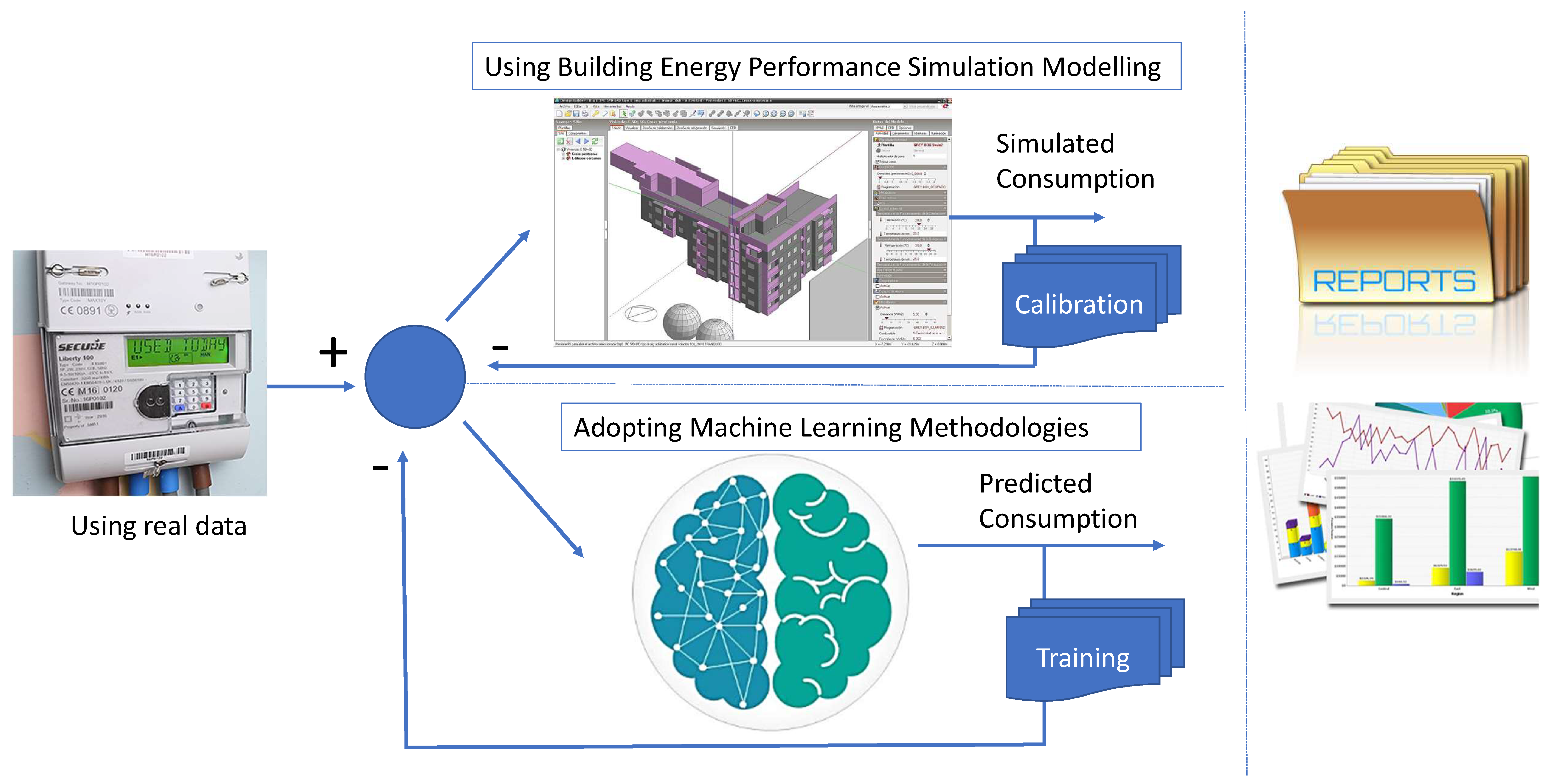
With the recent paradigm of accessing high amounts of data in buildings (energy consumptions records and also exogenous variables such as indoor/outdoor temperatures, relative humidity, or solar radiation), it becomes possible to take into account available data to predict future consumptions. In fact, it is the authors’ admitted research interest to assess whether machine learning prediction methods to estimate future load demand in buildings may provide an alternative of using common building energy simulation tools. This change in paradigm is illustrated in Figure 1.

Machine learning approaches, often called data-driven models, require a training stage comparable to the calibration stage in traditional simulation processes, mainly to determine the relative importance of different features used to estimate future load demand. The feature selection stage will be further explored in Section 3. While the training stage occurs, it is expected that estimated consumptions will be closer to real consumptions.

When using building energy dynamic simulation tools, sometimes the estimation of energy consumption is far from being coincident with reality when comparing simulations with measured data. The difference between these values is usually designated energy gap [13]. Reducing energy gap is an important issue to be taken into account when designing neutral energy buildings, since small differences in assumptions may result in higher energy performance gaps. Therefore, the use of data-driven approaches appears to be an important alternative to conventional building energy performance simulation tools in reducing the energy performance gap, since they do not rely on assumptions, but on historical data coming from buildings under operation conditions [14].

This study will focus on applying machine learning approaches to forecast thermal energy demand. Different researchers used forecasting models to predict building electricity demand [4,5,11,15]. It becomes clear that, in most cases, it is easier to obtain electrical energy as data with higher resolution, and also that quite often weather conditions can strongly influence these electricity consumptions (mainly during the summer periods, when air conditioning systems are used). Nevertheless, as the building analyzed in this article has its heating and cooling needs provided by district heating (further addressed in Section 2.1), electricity consumptions are quite more stable and easier to predict. For similar reasons, a considerable number of researchers are tackling the challenge of estimating building heating and cooling needs [3,5,15,16,17,18,19].

A number of studies can be found in the literature that address the forecast of energy demand of non-domestic buildings (both thermal and electrical) using machine learning strategies. In [20], artificial neural networks (ANN) are compared to a physical principle-based model (EnergyPlus) when forecasting the amount of energy consumed by an administrative building in São Paulo, Brazil. In [16], a load forecasting method using wavelet transform, SVM and partial least squares regression is applied to an office building in Tianjin, China. In [21], a linear regression model on air temperature data is compared to decision trees, SVM and ANN as they attempt to forecast the total heating energy demand of a set of 52 residential buildings. In [22], the effect of considering a single artificial intelligence based method or combining multiple single artificial intelligence based prediction models (ensemble approach) is also analyzed, trying to capture the benefits and avoid drawbacks associated with different strategies.

The article is organized as follows: Section 2 describes the dataset used for this study and presents some background related to the used methods and the strategies adopted when applying them in this study. Additionally, the adopted error metrics and the list of features considered to predict heating and cooling energy demands are also introduced. In Section 3 the main results are presented, with a feature selection stage followed by a detailed comparison among the proposed methods, for both seasons. Section 4 is dedicated to the discussion, revealing the potential amongst the forecasting models tested and highlighting a comparative analysis of these selected models. Finally, in Section 5, the main conclusions are drawn and some topics for further research are proposed.

2. Materials and Methods

In this section, the dataset information used for computing the models is presented, along with a brief overview of ANN, SVM and simulated annealing (SA) as a metaheuristic used to enhance SVM model. The work presented in this paper follows on from a previously published work by the same authors. [23].

2.1. Dataset, Model Characterisation, and Inputs

The case-study building for this paper is an office building on the riverside of a recently modernized district in Lisbon, Portugal. Built in 2007, it has a net floor area just under 12,000 m², with 7000 m² over eight floors (above ground) occupied by offices and open workspace area, and 5000 m² over three (underground) floors dedicated to parking. All building façades are mostly glazed and exposed to the elements, with partial shading installed on the south-facing façade only. The roof consists of a polystyrene insulated concrete slab covered by an outer layer of pebbles. The building is equipped with an advanced BMS, including a building automation and control system (BACS). A nearby trigeneration plant provides hot and cold fluids used to heat and/or cool the building, which are transferred through heat exchangers installed on a thermal substation located on the underground floors.

A significant amount of data was collected, including weather-related data (outdoor dry-bulb temperature, relative humidity, wind speed, direct normal solar radiation, diffuse horizontal radiation, occupation (hourly profile), and enthalpic counts of (hot and cold) fluid consumed from a complete year, obtained through simulation of a calibrated building energy performance model. In this area, the cooling period is usually April to September, while the rest of the year is the heating period. Around 4/5 of the data thus obtained was used in model training, while the remaining 1/5 was used for testing (heating and cooling) demand forecast. Both historical data (namely 7-days and 14-days prior) and exogenous variables were considered in the models. Variable normalization was performed, using training dataset maxima and minima for each variable as scaling factors.

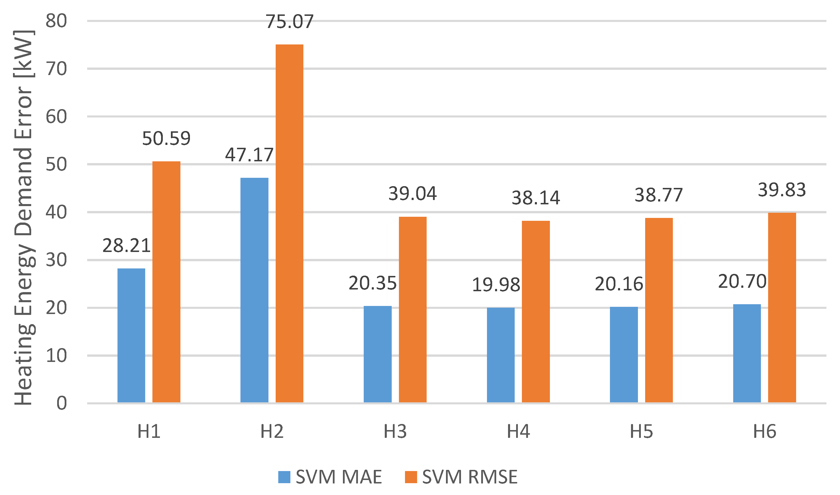
Different combinations of inputs were tested in this study and their respective error metrics (mean absolute error, MAE, and root-mean-square error, RMSE) were compared to evaluate the most effective set of inputs to forecast heating and cooling energy demand. In

Table 1. Sets of features tested for cooling energy demand forecast.

Feature	C1	C2	C3	C4	C5	C6
Historical cooling load from 1 week before [kW]	X		X	X	X	X
Historical cooling load from 2 weeks before [kW]	X		X	X	X	X
Outdoor air temperature [°C]		X	X	X	X	X
Relative humidity [%]		X			X	X
Estimated occupancy profile		X		X	X

and

Table 2. Sets of features tested for heating energy demand forecast.

Feature	H1	H2	H3	H4	H5	H6
Historical heating load from 1 week before [kW]	X		X	X	X	X
Historical heating load from 2 weeks before [kW]	X		X	X	X	X
Outdoor air temperature [°C]		X	X	X	X	X
Wind speed [m/s]		X
Direct normal solar radiation [kW]				X
Diffuse horizontal radiation [kW]					X
Relative humidity [%]		X				X

, the combinations of features tested for the cooling (Cx) and heating (Hx) energy demand, respectively, are presented.

2.2. Artificial Neural Networks

ANN are a well-known strategy to predict consumptions [24]. ANN are inspired by the way biological neurons of the human brain process information and are composed by several single and highly interconnected processors. An input node receives the contribution of adopted features and the last layer (the output layer) provides the information derived from the network (predicted values as the main goals of ANN for regression purposes). Between the input and output layer, one or more intermediate layers (hidden layers) are considered, and in these different number of neurons can be adopted, according to the real time series complexity. For each connection between elements, weights links are responsible to pass information signals from each unit to the next (respecting a feed-forward typology). A training stage is needed to provide the effectiveness of the model when comparing predicted values with the real ones. To do that, an error metric is used as an objective function that must be minimized in each iteration, sending the error to precedent layers and enabling a weights’ update (backpropagation).

Their ability to deal with non-linear relationships between inputs and outputs (possible when nonlinear transfer functions are adopted) and the option to predict different load records simultaneously (when adopting a single model multivariate forecasting) make ANN very suitable to forecast a daily load profile. For that reason, they are being adopted by several researchers to predict building energy consumptions [3,15,21]. Some drawbacks that are often pointed out are the inherent empirical process (based on trial-error experiments, mostly depending on random ANN parameters’ initialization), considerable risk of reaching local minima, and high dependence on a proper structure selection or even on a feature selection/extraction stage.

In this study, ANN were parameterized as follows:

• Hidden layer activation function: hyperbolic tangent;
• Weight optimization solver: “Adam”;
• Number of hidden layers: 1;
• Number of neurons: 40;
• Data training/validation ratio: 80%/20%.

The Adam optimization algorithm, which is an alternative to classical stochastic gradient descent, was used to update network weights since it is particularly efficient when handling large datasets, with a reasonable trade-off between training times and prediction accuracy. A single hidden layer was used as that is the most widely recommended choice to represent any type of function, with the approximation ability dependent on both the choice of activation functions and the number of neurons. The number of neurons was selected after ten-time ANN training trials using ten, twenty, thirty, forty and fifty neurons, following the best results (i.e., lowest error metrics); simulations with fewer neurons led to underfitting (lower ability to estimate heating/cooling), while higher number of neurons led to overfitting (generalization loss, lower ability to estimate new values). 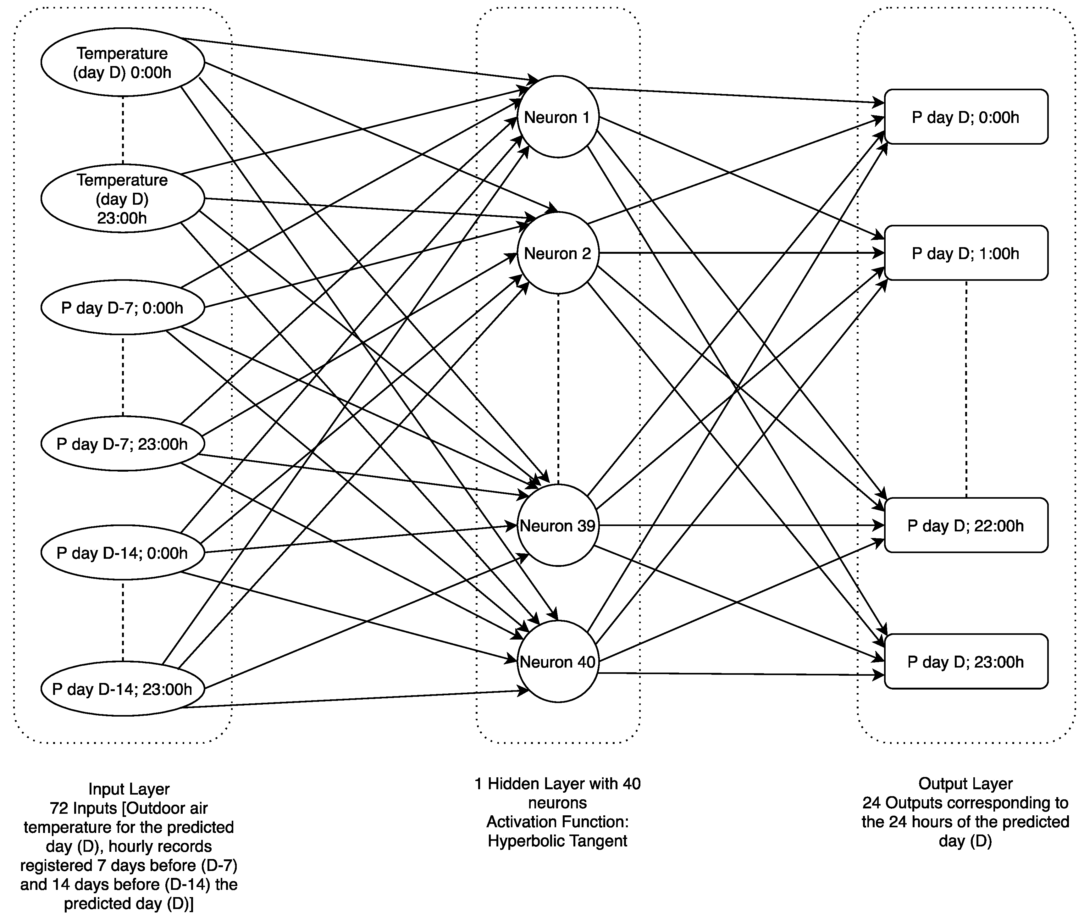Figure 2 presents an example of an ANN model’s structure based only on historical records (in this case, congenerous days, one week and two weeks before) and exogenous variables (in the example, temperature).

2.3. Support Vector Machines

While SVM have been widely used for classification purposes, the metaheuristic may also be applied to regression based on the same principles. It is consensual in the research community that this approach relies more on a structural risk minimization principle rather than an empirical risk minimization principle [16,25,26], quite common, for example, in ANN. Other particularity is that its training derives from quadratic programming, resulting in a global optimal solution. As it addresses a regression problem, SVM attempt to find an optimal hyperplane such that distance to data is minimized. The original input space is usually nonlinearly related to the predictor variable. Therefore, it is mapped onto a higher dimensional feature space through a nonlinear mapping function (kernel function) to deal with these nonlinearities. The kernel transformation allows the handling of nonlinear relationships in the data as a higher dimensional space is obtained, in which a linear regression model can be built.

An SVM model may be optimized by tuning the kernel function, the kernel parameter (gamma), the cost parameter, and the error margin (epsilon). The Radial Basis Function (RBF), which is commonly used in energy demand problems, is the kernel function best fit to deal with non-linearities. The level of non-linearity of an SVM model is defined, according to the width of the ensuing bell-shaped function (RBF). The cost parameter (C), used to apply a penalty on individual errors, is also important to avoid model overfitting.

The selection of the three non-negative parameters (epsilon, C, and gamma) is determinant to forecasting accuracy. The use of a combinatorial method is often suggested to optimize the parameter selection procedure [18,25,26,27,28]. The authors selected simulated annealing (SA) to approach the parameter selection stage.

A number of combinations were tested in an attempt to find the best-performing combination for the given dataset. The lowest values for error metrics MAE and RMSE were obtained for C = 500, gamma = 0.5 and epsilon = 0.5.

2.4. Simulated Annealing as a Metaheuristic Used to Enhance SVM Model Accuracy

SA is one of the oldest metaheuristics with an explicit strategy to avoid the problem of the local minima [26]. The subjacent idea is to allow the acceptance of some solutions that can eventually deteriorate the objective function, in order to keep away from local minima. The current solution is replaced by a new solution in a random neighborhood, and the extent of the search is based on a probability distribution with a scale that is proportional to the “temperature”. An annealing schedule is used to decrease the temperature as the algorithm proceeds. As the temperature decreases, the extent of its search is reduced to enable an approximation to a minimum. However, it is difficult to conclude whether this is the global minimum or an undesired local minimum. Thus, a reannealing process is often required. This reannealing process can be viewed as a supplementary strategy to a global search because the temperature in each dimension (for each variable) is raised, depending on temperature sensitivity, giving a wider opportunity to accept solutions that are distant from the aforementioned ones.

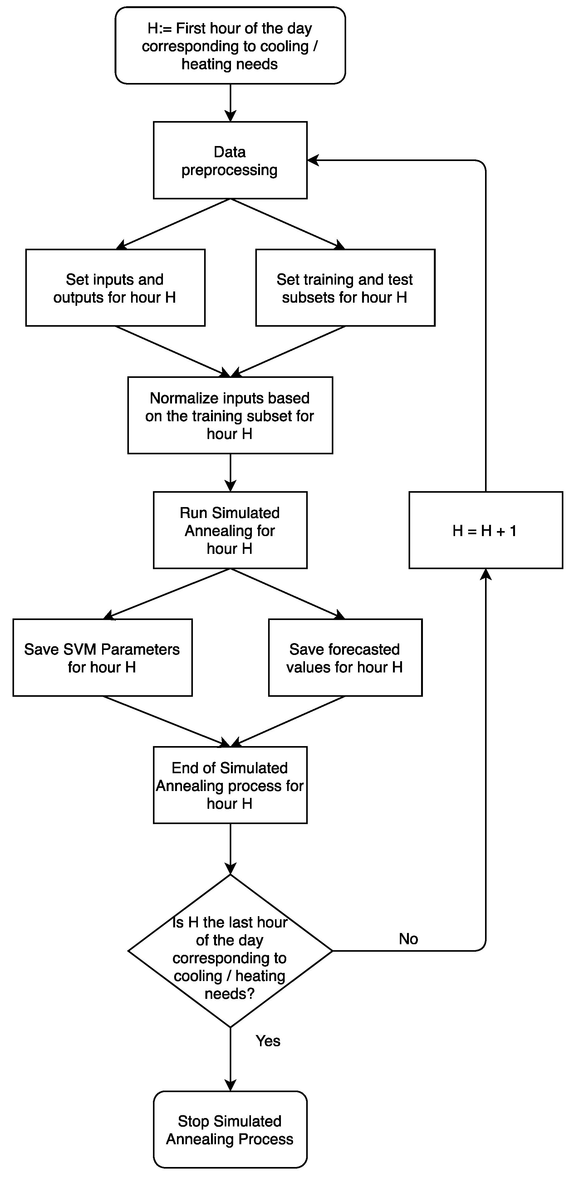
For this study, the SA approach to improve SVM models had some variations compared to the SVM models. Firstly, in order to be able to properly normalize the training and test subsets, only the hours in which heating and cooling systems were actually working were considered for the predictions; secondly, instead of a single combination of SVM parameters for all hours being predicted, each individual hour had its own combination, in order to allow SVM models to adapt to the time of the day at which prediction were made; and thirdly, also associated with the previous assumption, each hour being predicted is normalized using the minimum and maximum values registered in the training subset (unlike SVM, based on overall maximum and minimum).

Figure 3 shows the flowchart followed in this study when using SA to forecast hourly heating and cooling energy demand.

For the SA technique, thirty cycles (iterations) were used for each hour. In each cycle, fifteen trials, i.e., fifteen random initial combinations of SVM parameters were tested, and at the end of each cycle, the temperature would drop to narrow the range of options of each SVM parameter. The cost parameter C was tested in a range between 0 and 700, epsilon was tested between 0.0001 and 3, and gamma was tested between 0.0001 and 10. Other Simulated Annealing parameters were set as:

• Probability to accept a worst solution in the beginning (p₁) = 0.5;
• Probability to accept a worst solution in the last cycle (p₃₀) = 0.001;
• Initial temperature (t₁) = −1.0/log (p₁);
• Final temperature (t₃₀) = −1.0/log (p₃₀);
• Temperature for a new cycle (t_n) = (t₃₀/t₁)^[(1/(n−1)]·t_n−1, n being the number of the cycle.

The assumed objective function was based on the Root Mean Square Error (described in Section 2.5) verified in the validation subset (20% of the data, similar to the approach followed for ANN). An example of the optimization model being evaluated during thirty iterations is shown in Figure 4, where the objective function being minimized can be evaluated, while the acceptance of worse solutions and the exploitation of different parameters’ combination can also be appreciated.

2.5. Error Metrics

This section describes the error metrics used to evaluate the performance of the models. In this work, two error metrics were used to score and compare forecast values to reference values [29,30].

The mean absolute error (MAE) is obtained by computing the average absolute error between the reference values (y) and the predicted values (ŷ) through n observations (1):

$$\mathrm{MAE}=\frac{1}{n}.{\displaystyle \sum }_{i=1}^n\left|y_i-{\mathsf{ŷ}}_{\mathrm{i}}\right|.$$

(1)

The root mean squared error (RMSE) represents the mean standard deviation of the predicted values when compared to the reference values (2):

$$\mathrm{RMSE}=\sqrt{\frac{{{\displaystyle \sum }}_{i=1}^n{(y_i-{\mathsf{ŷ}}_{\mathrm{i}})}^2}{n}}.$$

(2)

3. Results

In this section, the results obtained using ANN, SVM, and SVM+SA to forecast cooling and heating energy demand are presented in three stages:

-

Feature selection, where the different sets of inputs characterized in Table 1 and Table 2 are tested and compared to select the best performing one according to their error metrics;

-

Models’ accuracy evaluation, in which the load profile that results of the best performing model selected in the previous stage is compared to the reference in a complete day of the test subset;

-

Error distribution analysis, where the error range of the best performing models’ forecasted values of the test subset is assessed for every hour in which the systems are working.

3.1. ANN Model

3.1.1. Feature Selection

In Figure 5, the error metrics for the models described in Table 1, using ANN, are presented.

By analyzing Figure 5, only based on MAE, C3 is the most accurate in forecasting cooling energy demand. However, as RMSE is more sensitive to highest errors, this was the main criteria in the selection of the best set of inputs. Therefore, based on this latter error metric, C2 (only based on exogenous variables) provided the most accurate predictions for cooling energy demand, closely followed by C3 and C6.

In Figure 6, error metrics for the sets of inputs tested for ANN models on forecasting heating energy demand are presented.

In the heating period, as in the cooling period, different assumptions can be taken by analyzing both MAE and RMSE. Considering MAE, H3 is the most accurate in forecasting heating energy demand but keep following the criteria considered in the cooling period, by analyzing RMSE, H4 provided the most accurate predictions for heating energy demand, with models H3, H5, and H6 also being very accurate in forecasting energy demand. The importance of using historical load data and outdoor air temperature can also be concluded, while direct normal solar radiation is a recommendable feature in this case. Another detail that stands out is that, by comparing Figure 5 (cooling period) with Figure 6 (heating period), both error metrics tend to be lower in the latter, meaning that it is easier for ANN models to predict energy demand in the heating season.

3.1.2. Models’ Accuracy Evaluation

Having selected the best set of input features for both the heating and the cooling periods, the following step is to evaluate ANN models’ accuracy by comparing their resulting forecasted values with heating and cooling energy data obtained from the case study building’s dynamic simulation model, used as reference. Figure 7 depicts a load profile comparison between ANN model C2 and the reference values, for a complete working day, for the test subset in the cooling period.

As it was depicted in Figure 7, ANN models are very accurate in forecasting cooling energy demand throughout the day, with the trend of predicted values being located below the reference.

Figure 8 presents a comparison between the load profile for ANN model H4 and the reference values, for a complete working day of the test subset, during the heating period.

Comparing forecasted values from the ANN model to the reference ones for the same day in the test subset, it is patent that the ANN model provides a fair approximation to the reference data.

3.1.3. Error Distribution

After evaluating the accuracy of the ANN models when compared to reference data, it is time to assess the error distribution for every hour heating or cooling systems are working.

Concerning to the cooling energy demand error distribution, Figure 9 presents the range of errors from 8:00 to 17:00, corresponding to the working hours of the cooling systems.

Analyzing the boxplot for cooling energy demand error (Figure 9), the highest deviations occur between 10:00 and 14:00, corresponding to the higher outside temperatures verified in that period. The median is located near 0 for every hour, with a higher percentage of the error above the median, meaning that the reference values tend to be higher than the values forecasted by the ANN models.

The boxplot with the error distribution for heating energy demand, for the working hours of the heating systems, is presented in Figure 10.

The error range for the heating energy demand, presented in Figure 10, is much lower than that for the cooling period. The highest deviations occur early in the morning and during the afternoon. As in Figure 9, the median is also located near 0 for every hour in which systems are working. From 07:00 to 18:00, the higher percentage error is located above the median, meaning that ANN models tend to underpredict heating energy demand. Towards the end of the day, the opposite happens, as the forecasted values tend to be higher than the reference values.

3.2. SVM Model

The same procedure previously followed when using ANN models was now applied to SVM models, starting with the feature selection stage, followed by the models’ accuracy evaluation and finally by the error distribution analysis.

3.2.1. Feature Selection

In Figure 11, the error metrics for the models described in Table 1 are presented for cooling demand forecast, using SVM.

Using SVM models for the cooling period, the most accurate set of inputs tested was C5, closely followed by C6.

In Figure 12, the error metrics for the models described in Table 2 are presented for heating energy demand forecast, using SVM.

By analyzing Figure 12, all combinations tested for the heating period using SVM presented similar results, except H1 (only based on historical records), and H2 (only based on exogenous variables), with model H4 slightly more accurate than the others. Overall, the exogenous variables’ influence in the heating period is more balanced, as models H3 to H6 had similar error metrics, whereas for the cooling period, relative humidity and estimated occupancy profile are more influent when predicting cooling energy demand.

3.2.2. Models’ Accuracy Evaluation

At this stage, SVM models’ forecast is confronted with reference values registered for a complete working day from the test subset. Figure 13 presents the load profile based on SVM forecasted values for the cooling period and the reference for that same day. Figure 13 shows that SVM models are quite effective in forecasting cooling energy demand.

The comparison between the values forecasted by SVM and the reference values, for the heating period, is presented in Figure 14.

For the heating period, Figure 14 shows that the load profile based on SVM forecasted values is close to the reference values, with some deviations mainly towards the later hours of the day.

3.2.3. Error Distribution

The error distribution for SVM predictions was also assessed. The cooling energy demand error distribution for SVM models is presented in Figure 15.

The boxplot for the cooling energy demand error distribution, represented in Figure 15, shows that most of the errors are located above 0 from 8:00 to 10:00, meaning that the reference values tend to be higher than those forecasted by SVM model C6 for those hours. For the remaining hours, forecasted values tend to be higher than the reference, as the error distribution is mostly negative.

A boxplot to evaluate the error distribution for forecasting heating energy demand using SVM models is presented in Figure 16.

The boxplot for the error distribution confirms the trend of the SVM models, which tend to underpredict heating energy demand, since most errors are located above 0. However, in the later working hours, this trend is reversed.

3.3. SVM+SA Model

In order to improve SVM models predictions, SA was used to optimize SVM parameters for the six models studied, both in the cooling and the heating periods.

3.3.1. Feature Selection Stage

In what concerns to the feature selection stage for the cooling period, Figure 17 presents the error metrics for models C1 to C6 using SVM models with the improvement of SA.

Comparing all six models tested for the cooling period, the error metrics regarding SVM+SA showed the same trend as those presented in Figure 11 (SVM without SA), with model C5 being again the most accurate model, followed by C6 and C4. The effect of SA in the error metrics is also noticeable when comparing Figure 17 to Figure 11, with considerable improvement in all models tested.

In Figure 18, the error metrics using SVM+SA models are presented for heating energy demand forecast.

In the heating period, the models show results similar to those obtained using only SVM (Figure 12), and so the same trend was evidenced using SVM+SA (Figure 18). As observed in the non-optimized SVM models (Figure 12), when using simulated annealing, model H4 also registered the most accurate predictions for heating load demand.

3.3.2. Models’ Accuracy Evaluation

In this stage, SVM models’ predictions with SA improvement are compared to reference values both for cooling and heating energy demand. Starting with the cooling period, the load profile for SVM models with SA for a complete working day from the test subset is presented in Figure 19.

Figure 19 shows that SVM models with SA are very accurate in forecasting cooling energy demand, as the projected load profile is very similar to the reference. Moreover, as stated in the feature selection stage, the improvement in the load profile matching in Figure 19, when compared to the load profile without SA, in Figure 13, is also noticeable.

In Figure 20, the load profile of forecasted values based on SVM models with SA for the heating period is presented and compared to the reference values.

Just as it had in the cooling period (Figure 19), SA proved to be a major improvement to SVM models in the heating period, with the load profile for the predicted values almost identical to the reference with only one major variation occurring at 7:00.

3.3.3. Error Distribution

The error distribution for SVM models with SA optimization was analyzed using boxplot charts, starting with the cooling period presented in Figure 21.

The boxplot with the error distribution for the cooling period based on SVM models with SA shows that the range of errors for every hour is much lower than that in Figure 15 (based on SVM without SA). Most of the errors are located above 0, except at 8:00 and 17:00, meaning that SVM models tend to underpredict cooling energy demand, as they had in Figure 15.

The boxplot with the error distribution for the forecasted values regarding heating energy demand, based on SVM models with SA, is presented in Figure 22.

Figure 22 shows that the error range is, once again, much smaller than in Figure 16, due to the use of SA, and the trend of SVM models to underpredict heating energy demand is kept.

4. Discussion

After scrutinizing the results for the developed models in both cooling and heating periods, it is now convenient to evaluate which are the most accurate models overall in forecasting cooling and heating energy demand, respectively.

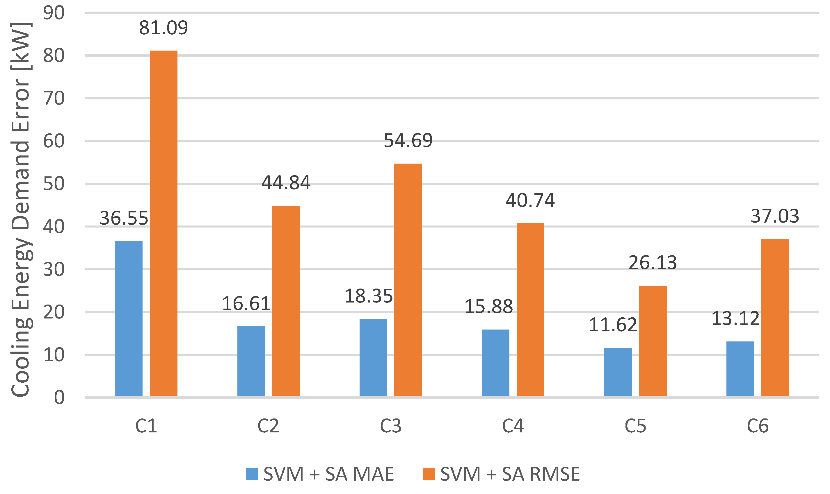
Concerning cooling energy demand, from the six models tested (represented in Table 1 using ANN, SVM and SVM with SA, the most accurate model, i.e., the one with the lowest MAE and RMSE, was C6 using SVM with SA. This means that the set of features that included historical cooling load, outdoor air temperature, relative humidity and estimated occupancy profile was the most effective in forecasting cooling energy demand.

4.1. Comparative Analysis

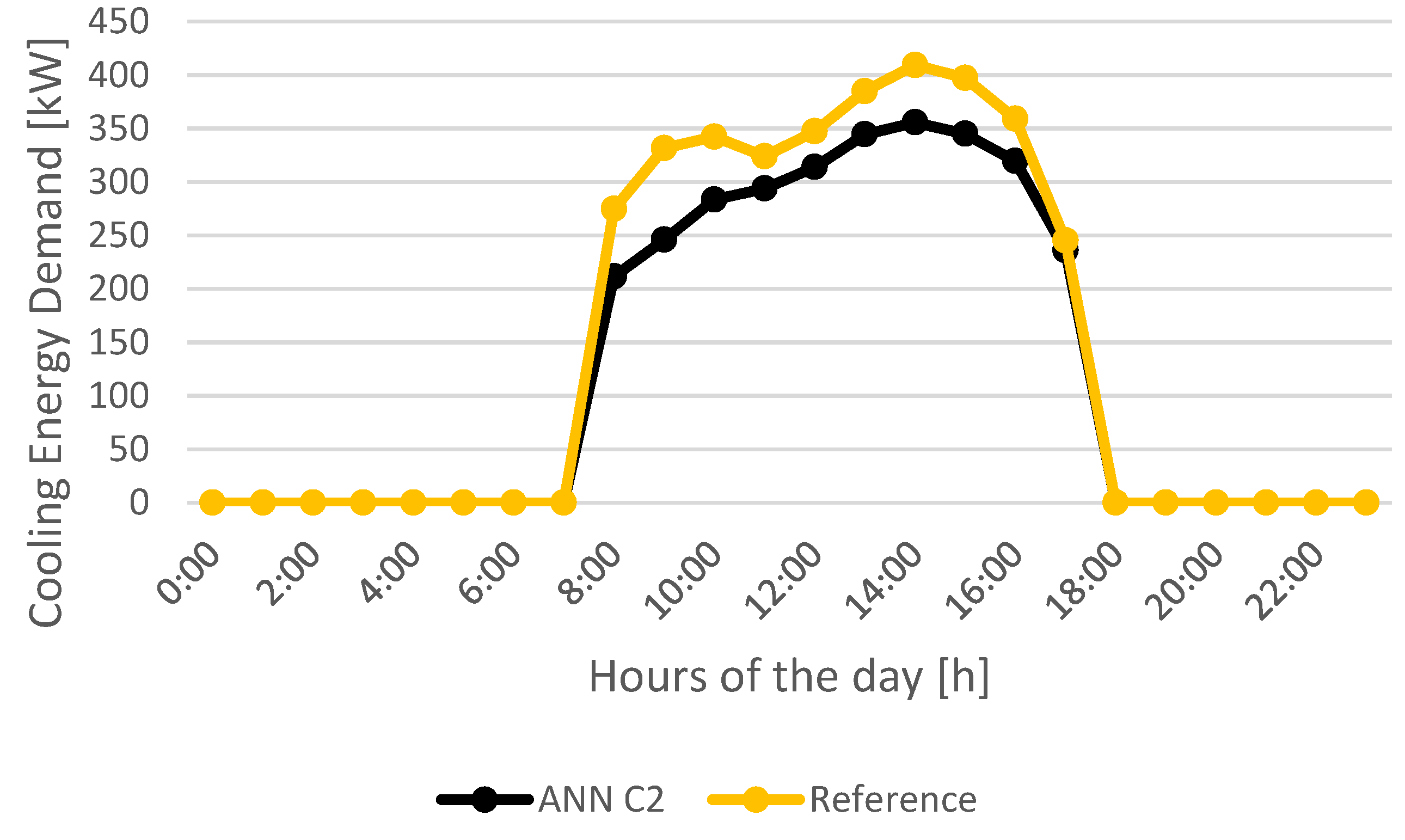
To compare the best performing models retrieved from each of the three different techniques studied (ANN, SVM and SVM+SA) in forecasting cooling and heating energy demand, a weekly load profile corresponding to the test subset was created in order to evaluate the aptitude of those models in fulfilling their goal.

Figure 23 presents weekly load profiles for ANN_C2, SVM_C5, and SVM+SA_C5 and reference for the cooling period.

By analyzing Figure 23, model SVM+SA_C5 provides the most accurate of the load profiles when compared to the reference.

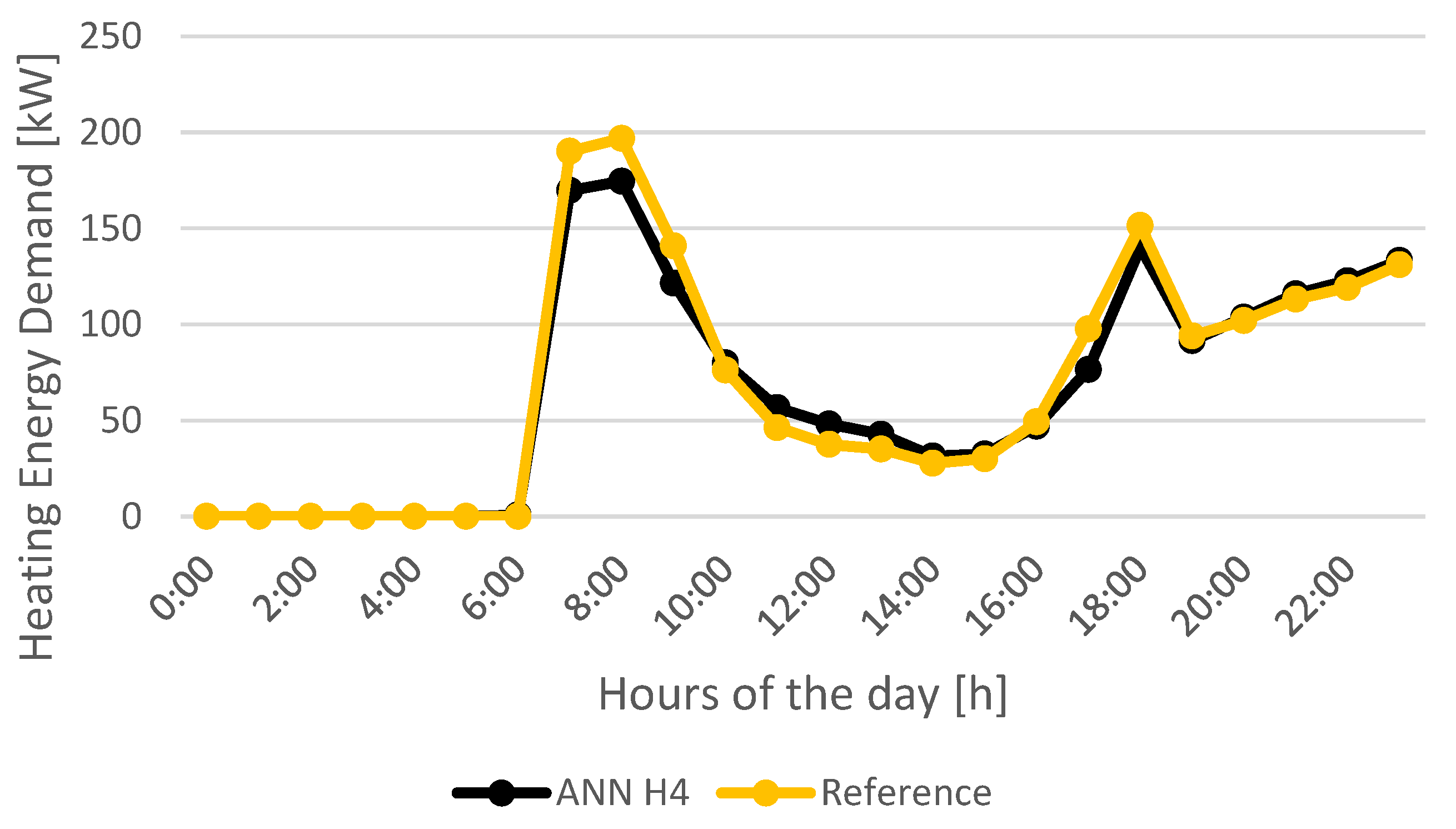
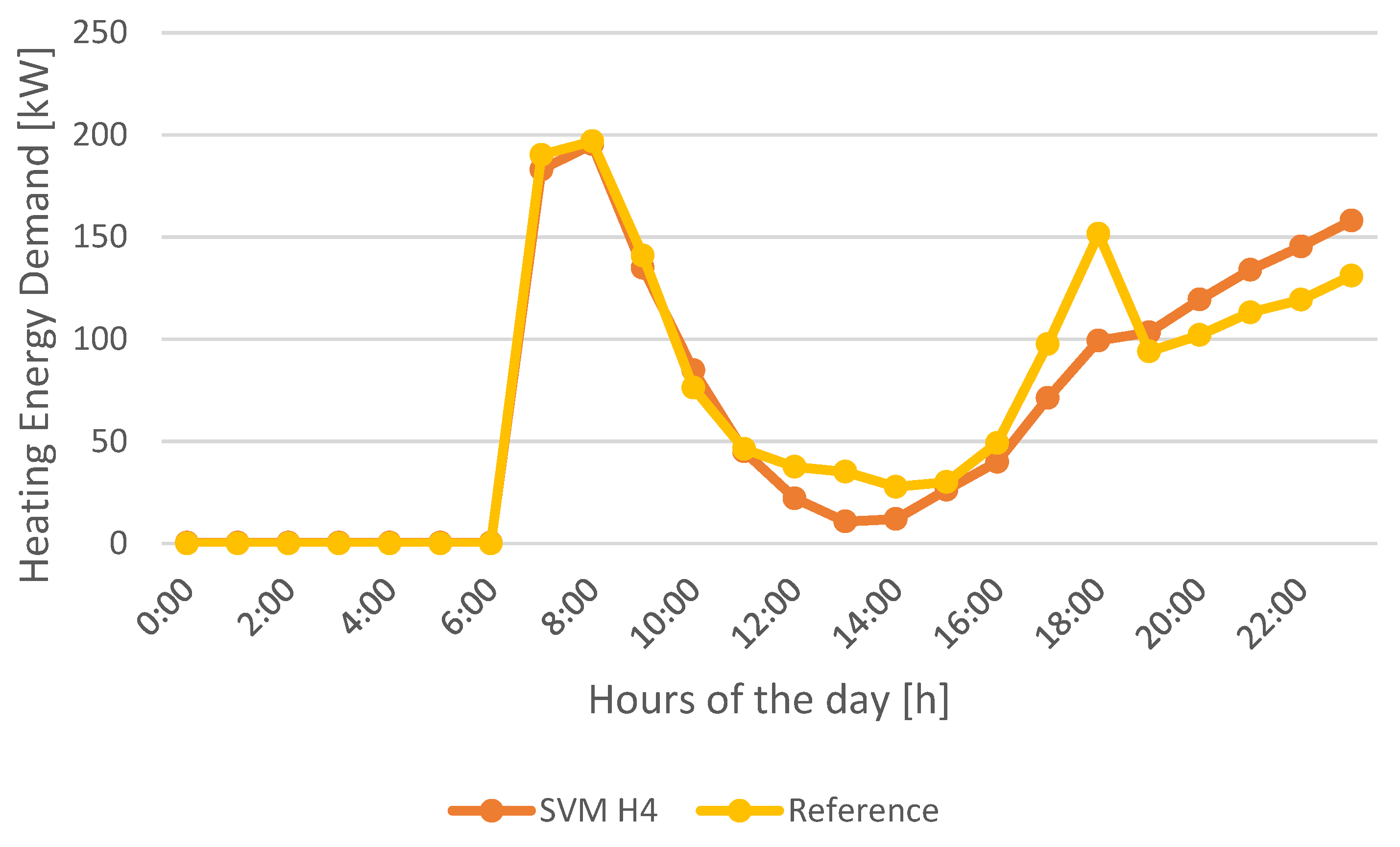
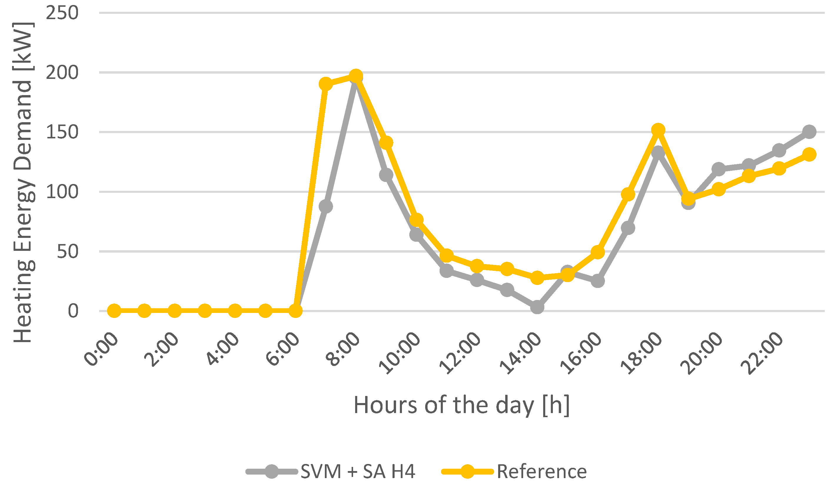
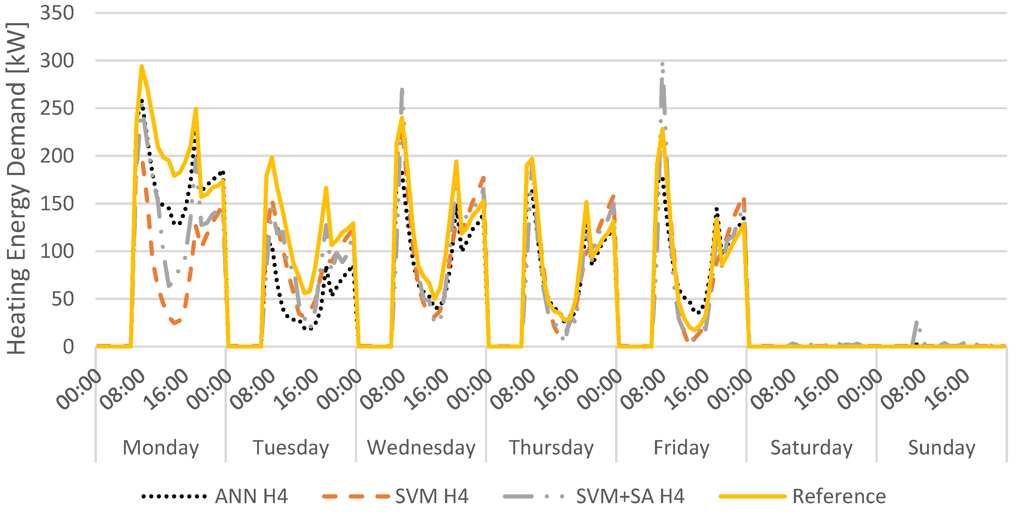
The weekly load profiles regarding heating energy demand for the best performing models in each machine learning technique studied are presented in Figure 24.

Analyzing the weekly load profiles for heating energy demand forecast (Figure 24), the most precise model is ANN_H4. Especially when analyzing the peaks registered in the morning and afternoon from Monday to Friday, model ANN_H4 is the model that best fits the reference profile.

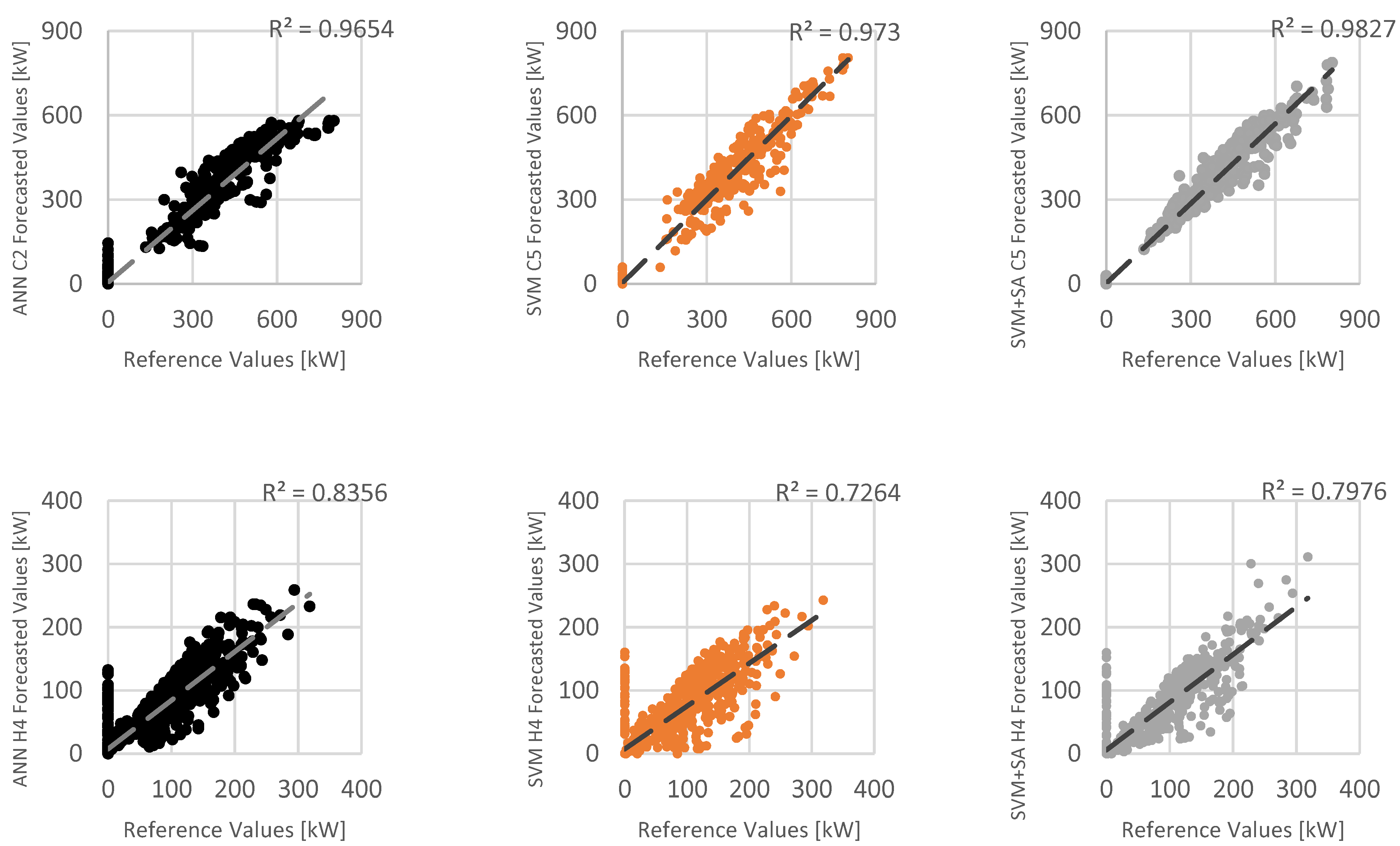
4.2. Forecast vs. Reference

In this section, a detailed comparison, for the full testing subset, between the forecasted values for all three models and the respective reference values is presented, using a dispersion chart. Figure 25 presents the dispersion chart for the cooling energy demand (ANN_C2, SVM_C5 and SVM+SA_C5) and the heating energy demand (ANN_H4, SVM_H4 and SVM+SA_H4) and the corresponding correlation factors (R²).

For the cooling period (the top three charts), all models have a very high correlation between the forecasted values and the reference values. The dispersion is slightly higher for ANN_C2, while SVM+SA_C5 presents a very high concentration of the points around the trendline with a R² of 0.9879.

For the heating period, the correlation factors are lower than in the cooling period. This may be partly due to the fact that the Christmas season is part of the testing subset and the models are not configured to detect holidays, considering them as normal working days. The highest correlation factor is obtained for the ANN_H4 model, which confirms it as the most effective model in forecasting heating energy demand. Moreover, the trendlines for the three bottom models are considerably below the bisector of the chart, meaning that, in all these models, most of the forecasted values for heating energy demand are lower than the respective reference values.

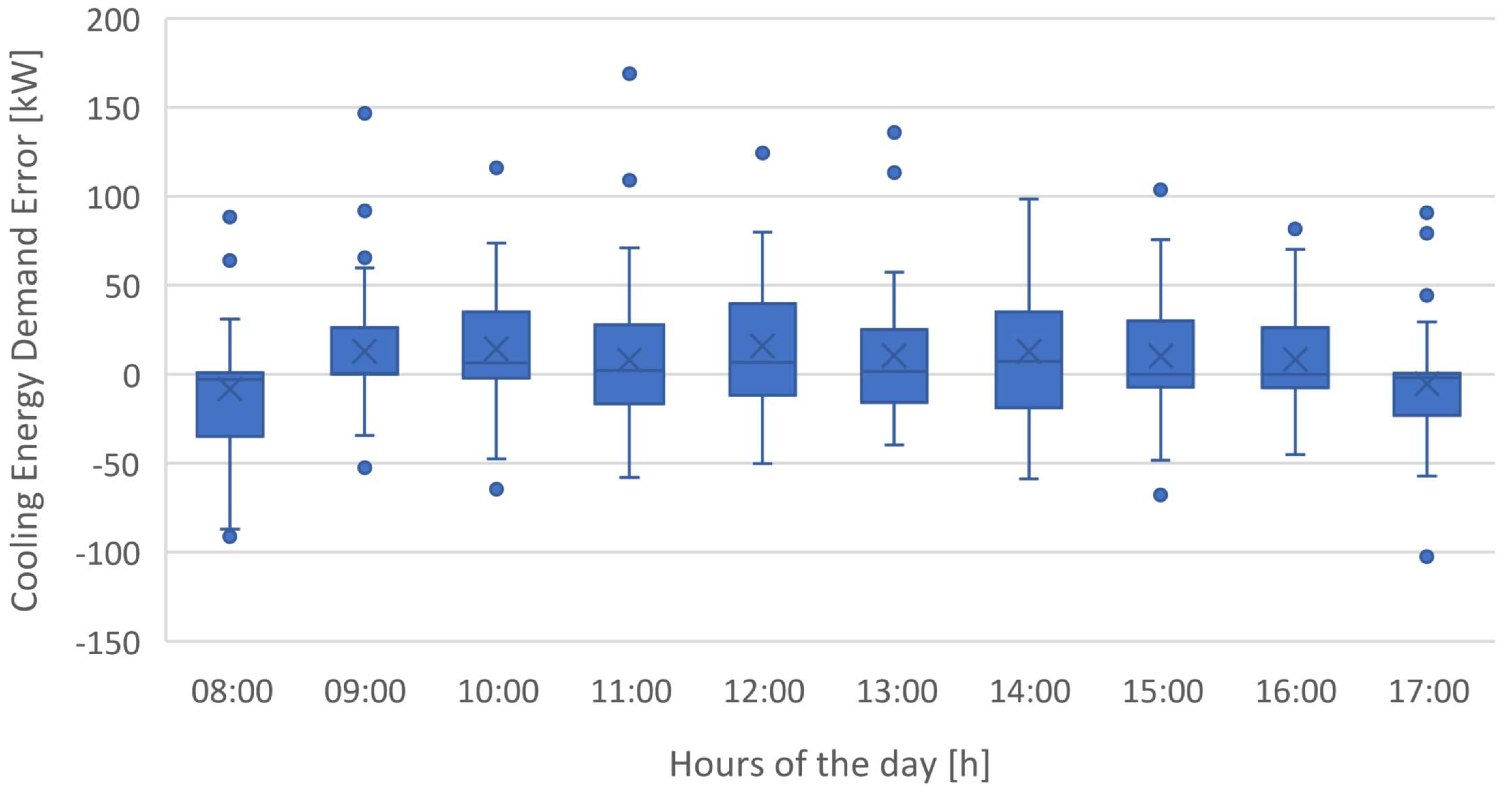
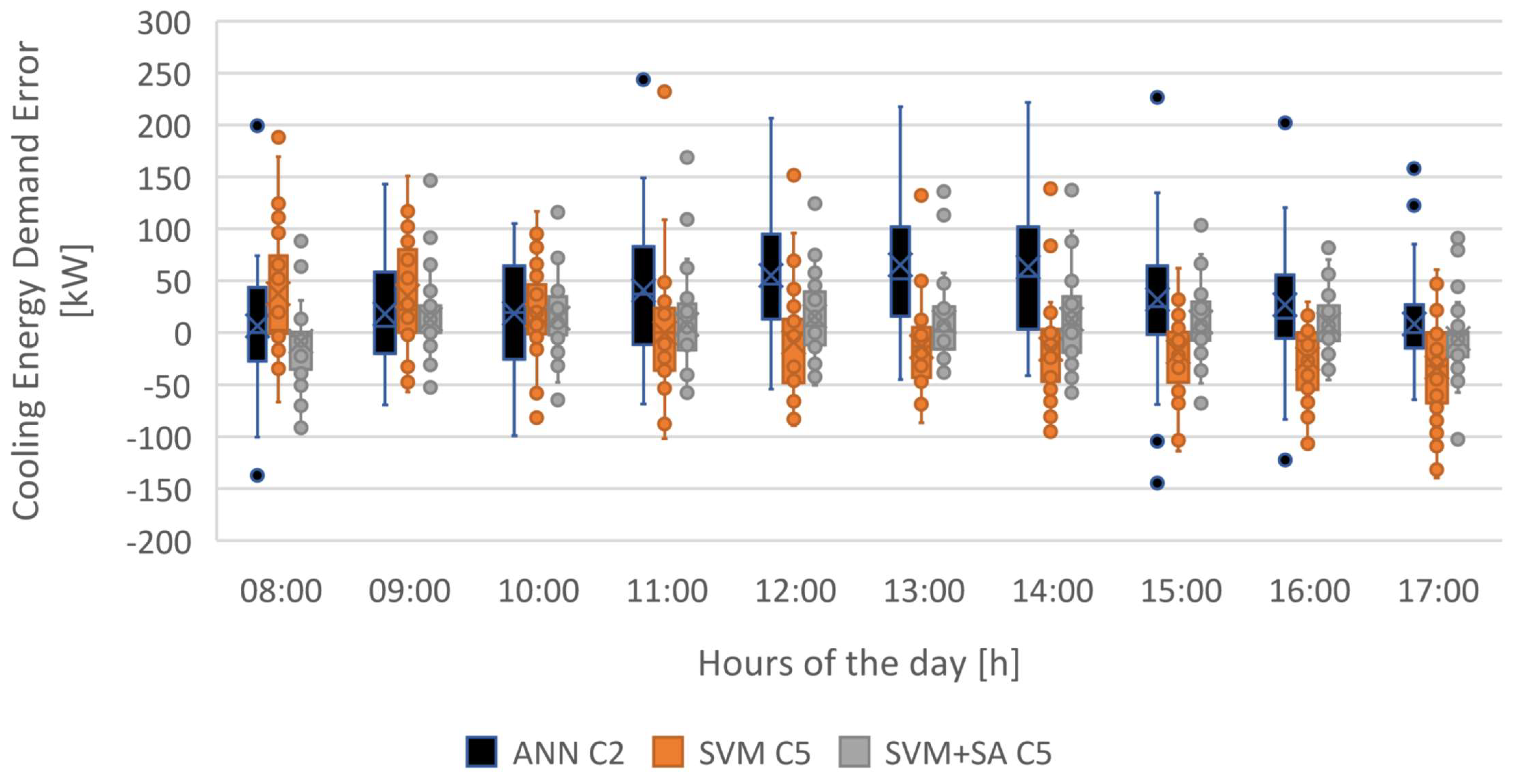
4.3. Boxplot Analysis

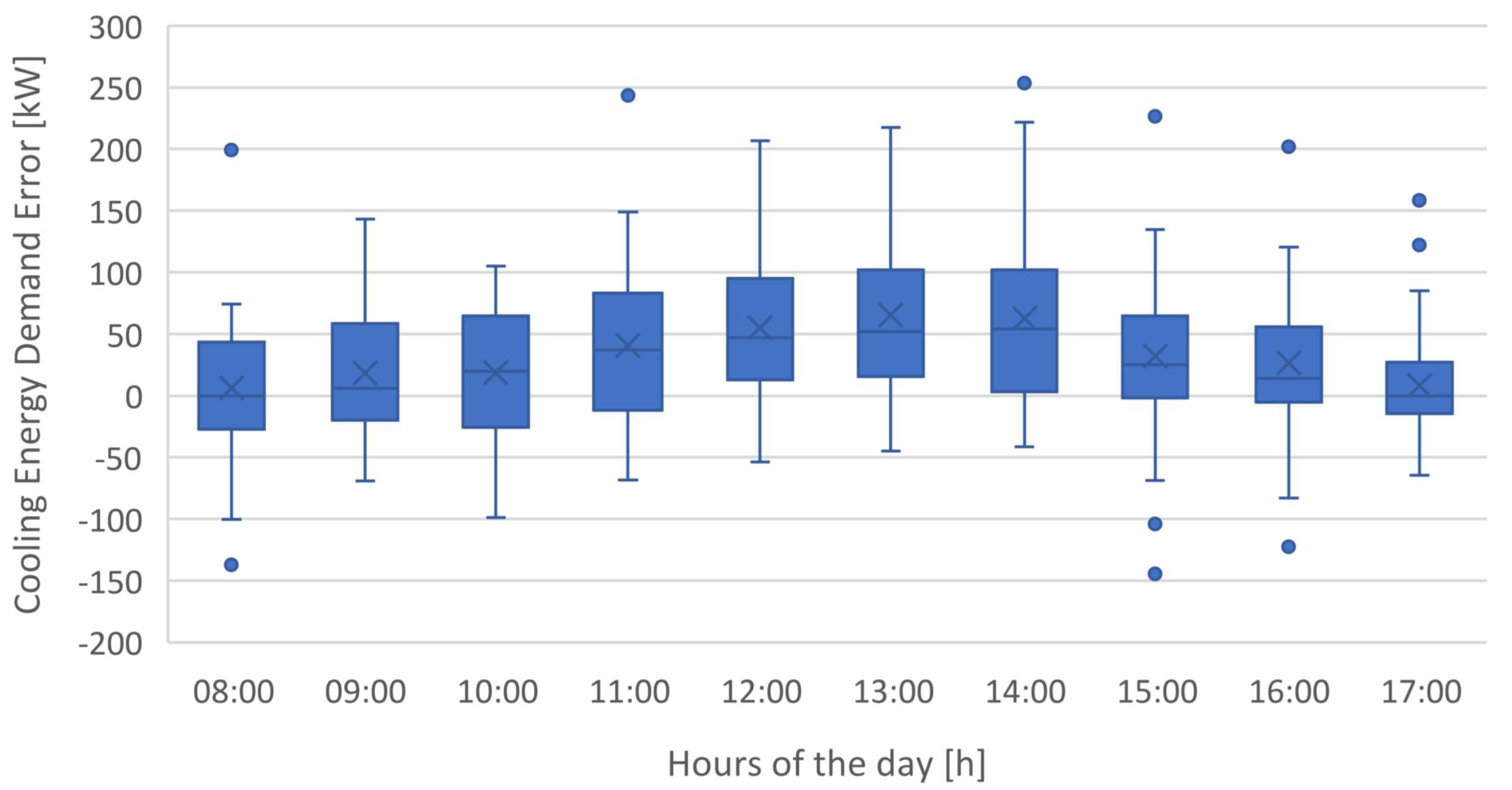
In this section, the error distributions for the best performing models of each machine learning strategy studied are presented and compared.

Figure 26 presents the boxplot chart containing the error distributions for models ANN_C2, SVM_C5 and SVM+SA_C5 in forecasting cooling energy demand, while

Table 3. Statistical parameters for cooling energy demand error.

Statistical Parameter [kW]		ANN_C2				SVM_C5				SVM+SA_C5
		8 a.m.	12 p.m.	8 p.m.		8 a.m.	12 p.m.	8 p.m.		8 a.m.	12 p.m.	8 p.m.
Mean		6.35	55.08	26.73		37.68	−9.22	−24.96		−8.36	15.84	8.48
Std. deviation		44.03	48.82	50.36		49.82	39.25	31.22		30.55	31.97	23.80
Minimum		−136.91	−53.89	−122.37		−66.41	−89.04	−110.99		−91.29	−50.14	−45.15
1st Quartile		−26.56	16.47	−3.95		−0.69	−43.78	−50.29		−30.73	−10.78	−5.71
Median		0.00	46.76	14.10		2.54	-0.61	−7.57		−3.05	6.73	0.00
3rd Quartile		43.22	90.88	52.95		72.58	11.31	0.00		0.07	36.13	25.06
Maximum		199.07	206.50	207.00		188.11	151.70	29.55		92.94	126.39	81.62

highlights some statistical parameters for particular hours of the day.

Once again, and confirming the information given by Figure 23 and Figure 25, the error distribution shows that the most effective model in forecasting cooling energy demand is model C5, using SVM+SA.

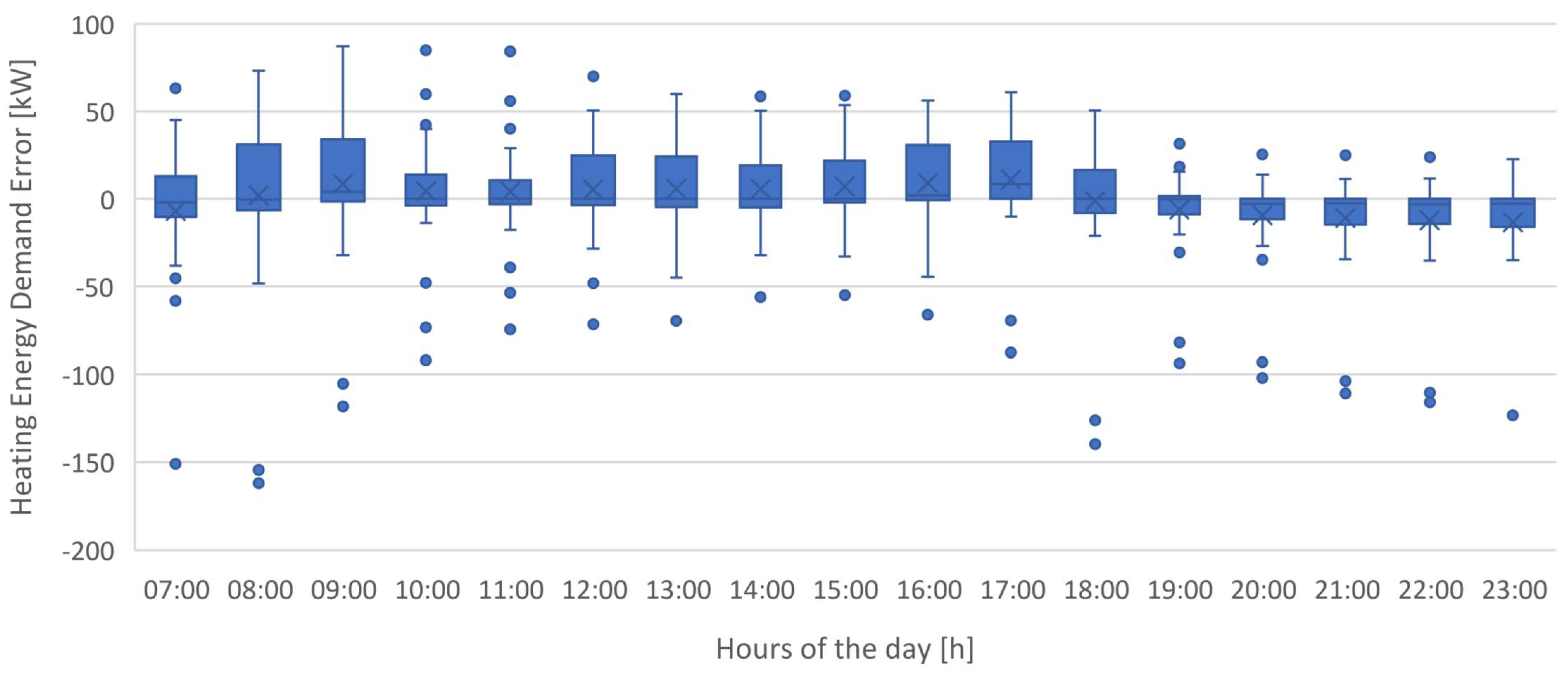
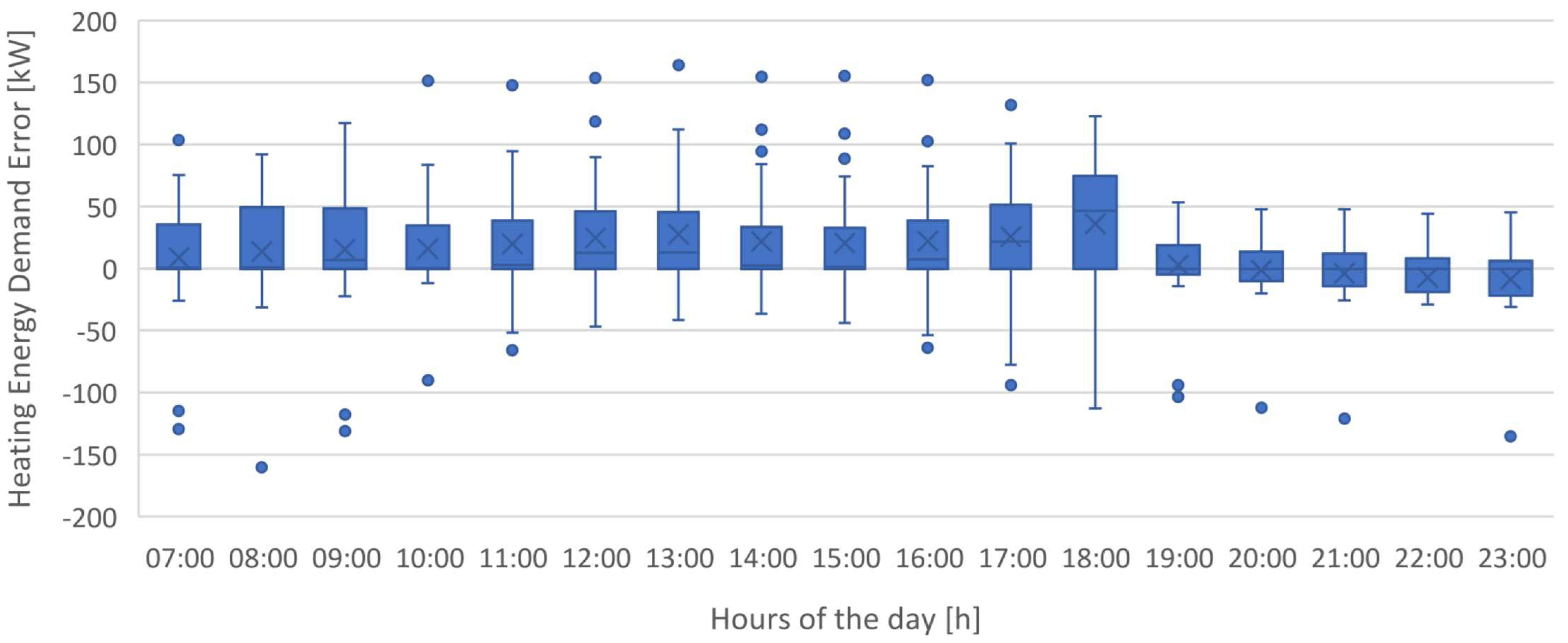
Figure 27 presents the error distribution for models ANN_H4, SVM_H4 and SVM+SA_H4 in forecasting heating energy demand, while

Table 4. Statistical parameters for heating energy demand error.

Statistical Parameter [kW]		ANN_H4				SVM_H4				SVM+SA_H4
		8 a.m.	12 p.m.	8 p.m.		8 a.m.	12 p.m.	8 p.m.		8 a.m.	12 p.m.	8 p.m.
Mean		2.03	5.41	−9.30		13.44	24.72	−1.49		0.24	13.99	−1.22
Std. deviation		29.96	18.57	15.21		36.52	31.78	18.48		29.57	23.24	17.93
Minimum		−162.04	−71.67	−102.12		−160.18	−46.90	−112.25		−159.73	−60.42	−108.59
1st Quartile		−5.42	−3.26	−11.38		−0.51	−0.50	−9.68		−4.71	−3.47	−5.81
Median		−0.35	0.00	−2.71		0.99	12.48	−0.49		−1.00	7.04	−2.97
3rd Quartile		29.80	22.58	0.00		46.25	42.99	12.84		17.69	23.71	16.87
Maximum		73.07	69.95	25.50		92.05	153.69	47.58		84.50	104.52	46.77

highlights some statistical parameters for particular hours of the day.

Figure 27 and Table 4 show that model ANN_H4 has an overall more satisfactory error distribution than models SVM_H4 and SVM+SA_H4, confirming the information given by Figure 24 and Figure 25.

It must also be pointed out that a generalized improvement in prediction accuracy occurs when SA is adopted in SVM models.

5. Conclusions

This article presents the application of different machine learning methodologies to estimate thermal energy demands in an office building. The proposed methodology was tested using a real office building located in Lisbon, Portugal, as a case study.

The demand forecast obtained from these methods proved to be an interesting alternative to the use of dynamic simulation tools, since it is certainly a quicker and more straightforward approach (less dependent on calibration processes and on expertise level of the user). Based on these results, there is a potential for faster, yet accurate machine-learning based forecasting methods to actually replace well-established, very accurate but time-consuming multi-zone dynamic simulation tools, allowing new possibilities of obtaining quick building energy consumption forecasts.

One of the contributions to the research field is related to the integration of SA as a strategy to support the fine-tuning of SVM’ parameters. In the previous sections, this addition proved to be quite effective, as it contributes to reduce prediction errors when compared to the SVM model (for both cooling and heating periods). Another relevant contribution is the evaluation on the impact of different sets of features, contributing to infer the most relevant ones for each season.

Future work may include the adoption of pre-processing techniques (e.g., the wavelet transform) in an attempt to improve model accuracy, particularly concerning the cooling period.

References

1. Fallah, S.; Deo, R.; Shojafar, M.; Conti, M.; Shamshirband, S. Computational Intelligence Approaches for Energy Load Forecasting in Smart Energy Management Grids: State of the Art, Future Challenges, and Research Directions. Energies 2018, 11, 596. [Google Scholar] [CrossRef] [Green Version]
2. Oliveira, F.; Bernardo, H. Energy Management Tools for Sustainability. In Encyclopedia of Sustainability in Higher Education; Filho, W.L., Ed.; Springer Nature: Berlin/Heidelberg, Germany, 2019. [Google Scholar]
3. Jang, J.; Lee, J.; Son, E.; Park, K.; Kim, G.; Lee, J.H.; Leigh, S.-B. Development of an Improved Model to Predict Building Thermal Energy Consumption by Utilizing Feature Selection. Energies 2019, 12, 4187. [Google Scholar] [CrossRef] [Green Version]
4. de Wilde, P.; Martinez-Ortiz, C.; Pearson, D.; Beynon, I.; Beck, M.; Barlow, N. Building simulation approaches for the training of automated data analysis tools in building energy management. Adv. Eng. Inform. 2013, 27, 457–465. [Google Scholar] [CrossRef]
5. Bourdeau, M.; Zhai, X.Q.; Nefzaoui, E.; Guo, X.; Chatellier, P. Modeling and forecasting building energy consumption: A review of data-driven techniques. Sustain. Cities Soc. 2019, 48, 101533. [Google Scholar] [CrossRef]
6. Schibuola, L.; Scarpa, M.; Tambani, C. Performance optimization of a demand controlled ventilation system by long term monitoring. Energy Build. 2018, 169, 48–57. [Google Scholar] [CrossRef]
7. Saheb, Y.; Shnapp, S.; Paci, D. From Nearly-Zero Energy Buildings to Net-Zero Energy Districts—Lessons Learned from Existing EU Projects; Publications Office of the European Union: Luxembourg, 2019. [Google Scholar]
8. Bernardo, H.; Martins, A.G. Resource-efficient nondomestic buildings: Intertwining behaviour and technology. In Energy and Behaviour: Towards a Low Carbon Future; Lopes, M., Antunes, C.H., Janda, K.B., Eds.; Academic Press: Cambridge, MA, USA; Elsevier: Amsterdam, The Netherlands, 2019; pp. 109–127. ISBN 9780128185674. [Google Scholar]
9. Kneifel, J.; Webb, D. Predicting energy performance of a net-zero energy building: A statistical approach. Appl. Energy 2016, 178, 468–483. [Google Scholar] [CrossRef]
10. Kalogirou, S.A.; Bojic, M. Artificial neural networks for the prediction of the energy consumption of a passive solar building. Energy 2000, 25, 479–491. [Google Scholar] [CrossRef]
11. Fathi, S.; Srinivasan, R.; Fenner, A.; Fathi, S. Machine learning applications in urban building energy performance forecasting: A systematic review. Renew. Sustain. Energy Rev. 2020, 133, 110287. [Google Scholar] [CrossRef]
12. Ahmad, T.; Chen, H.; Guo, Y.; Wang, J. A comprehensive overview on the data driven and large scale based approaches for forecasting of building energy demand: A review. Energy Build. 2018, 165, 301–320. [Google Scholar] [CrossRef]
13. Paone, A.; Bacher, J.-P. The Impact of Building Occupant Behavior on Energy Efficiency and Methods to Influence It: A Review of the State of the Art. Energies 2018, 11, 953. [Google Scholar] [CrossRef] [Green Version]
14. De Wilde, P. The gap between predicted and measured energy performance of buildings: A framework for investigation. Autom. Constr. 2014, 41, 40–49. [Google Scholar] [CrossRef]
15. Seyedzadeh, S.; Rahimian, F.P.; Glesk, I.; Roper, M. Machine learning for estimation of building energy consumption and performance: A review. Vis. Eng. 2018, 6, 5. [Google Scholar] [CrossRef]
16. Zhao, J.; Liu, X. A hybrid method of dynamic cooling and heating load forecasting for office buildings based on artificial intelligence and regression analysis. Energy Build. 2018, 174, 293–308. [Google Scholar] [CrossRef]
17. Deb, C.; Eang, L.S.; Yang, J.; Santamouris, M. Forecasting Energy Consumption of Institutional Buildings in Singapore. Procedia Eng. 2015, 121, 1734–1740. [Google Scholar] [CrossRef] [Green Version]
18. Xuemei, L.; Lixing, D.; Lanlan, L. A novel building cooling load prediction based on SVR and SAPSO. In Proceedings of the 2010 International Symposium on Computer, Communication, Control and Automation (3CA), Tainam, Taiwan, 5–7 May 2010; Volume 1, pp. 528–532. [Google Scholar] [CrossRef]
19. Powell, K.M.; Sriprasad, A.; Cole, W.J.; Edgar, T.F. Heating, cooling, and electrical load forecasting for a large-scale district energy system. Energy 2014, 74, 877–885. [Google Scholar] [CrossRef]
20. Neto, A.H.; Fiorelli, F.A.S. Comparison between Detailed Model Simulation and Artificial Neural Network for Forecasting Building Energy Consumption. Elsevier 2008, 40, 2169–2176. [Google Scholar] [CrossRef]
21. Saloux, E.; Candanedo, J.A. Forecasting District Heating Demand using Machine Learning Algorithms. Energy Procedia 2018, 149, 59–68. [Google Scholar] [CrossRef]
22. Wang, Z.; Srinivasan, R.S. A review of artificial intelligence based building energy use prediction: Contrasting the capabilities of single and ensemble prediction models. Renew. Sustain. Energy Rev. 2017, 75, 796–808. [Google Scholar] [CrossRef]
23. Godinho, X.; Bernardo, H.; Oliveira, F.; Sousa, J.C. de Forecasting Heating and Cooling Energy Demand in an Office Building using Machine Learning Methods. In Proceedings of the 2020 International Young Engineers Forum (YEF-ECE), Caparica, Portugal, 3 July 2020; pp. 1–6. [Google Scholar]
24. Runge, J.; Zmeureanu, R. Forecasting Energy Use in Buildings Using Artificial Neural Networks: A Review. Energies 2019, 12, 3254. [Google Scholar] [CrossRef] [Green Version]
25. Pai, P.-F.; Hong, W.-C. Support vector machines with simulated annealing algorithms in electricity load forecasting. Energy Convers. Manag. 2005, 46, 2669–2688. [Google Scholar] [CrossRef]
26. Sousa, J.C.; Jorge, H.M.; Neves, L.P. Short-term load forecasting based on support vector regression and load profiling. Int. J. Energy Res. 2014, 38, 350–362. [Google Scholar] [CrossRef]
27. Abbas, S.M.; Arif, M. Electric Load Forecasting Using Support Vector Machines Optimized by Genetic Algorithm. In Proceedings of the 2006 IEEE International Multitopic Conference, Islamabad, Pakistan, 23–24 December 2006; pp. 395–399. [Google Scholar]
28. Lin, S.-W.; Lee, Z.-J.; Chen, S.-C.; Tseng, T.-Y. Parameter determination of support vector machine and feature selection using simulated annealing approach. Appl. Soft Comput. 2008, 8, 1505–1512. [Google Scholar] [CrossRef]
29. Hippert, H.S.; Pedreira, C.E.; Souza, R.C. Neural networks for short-term load forecasting: A review and evaluation. IEEE Trans. Power Syst. 2001, 16, 44–55. [Google Scholar] [CrossRef]
30. Zuniga-Garcia, M.A.; Santamaría-Bonfil, G.; Arroyo-Figueroa, G.; Batres, R. Prediction interval adjustment for load-forecasting using machine learning. Appl. Sci. 2019, 9, 5269. [Google Scholar] [CrossRef] [Green Version]
Figure 1. Comparing paradigms related to building energy performance simulation tools and machine learning adoption.
Applsci 11 01356 g001
Figure 2. Representation of the multivariable artificial neural network adopted.
Applsci 11 01356 g002
Figure 3. Simulated annealing (SA) flowchart depicting approach used to enhance support vector machines (SVM) models.
Applsci 11 01356 g003
Figure 4. SVM parameters’ optimization during the SA process.
Applsci 11 01356 g004
Figure 5. Error metrics for cooling energy demand using artificial neural networks (ANN).
Applsci 11 01356 g005
Figure 6. Error metrics for heating energy demand using ANN.
Applsci 11 01356 g006
Figure 7. Daily load profile (13 September) comparison between ANN model C2 and reference for the cooling period.
Applsci 11 01356 g007
Figure 8. Daily load profile (19 December) comparison between ANN model H4 and reference for the heating period.
Applsci 11 01356 g008
Figure 9. Cooling energy demand error distribution during the test period using ANN.
Applsci 11 01356 g009
Figure 10. Heating energy demand error distribution during the test period using ANN.
Applsci 11 01356 g010
Figure 11. Error metrics for cooling energy demand using SVM.
Applsci 11 01356 g011
Figure 12. Error metrics for heating energy demand using SVM.
Applsci 11 01356 g012
Figure 13. Daily load profile (13 September) comparison between SVM model C5 and reference for the cooling period.
Applsci 11 01356 g013
Figure 14. Daily load profile (19 December) comparison between SVM model H4 and reference for the heating period.
Applsci 11 01356 g014
Figure 15. Cooling energy demand error distribution during the test period using SVM.
Applsci 11 01356 g015
Figure 16. Heating energy demand error distribution during the test period using an SVM model.
Applsci 11 01356 g016
Figure 17. Error metrics for cooling energy demand using SVM+SA.
Applsci 11 01356 g017
Figure 18. Error metrics for heating energy demand using SVM+SA.
Applsci 11 01356 g018
Figure 19. Load profile comparison between SVM+SA model C5 and reference for the cooling period.
Applsci 11 01356 g019
Figure 20. Load profile comparison between SVM+SA model H4 and reference for the heating period.
Applsci 11 01356 g020
Figure 21. Cooling energy demand error distribution for the test period using SVM+SA.
Applsci 11 01356 g021
Figure 22. Heating energy demand error distribution for the test period using SVM+SA.
Applsci 11 01356 g022
Figure 23. Cooling energy demand load profile for the best performing models, for a full week, from the test subset.
Applsci 11 01356 g023
Figure 24. Heating energy demand load profile for the best performing models, for a full week, from the test subset.
Applsci 11 01356 g024
Figure 25. Dispersion chart of forecasted values vs. reference for cooling period (top) and heating period (bottom).
Applsci 11 01356 g025
Figure 26. Error distribution for the best performing models in the cooling period.
Applsci 11 01356 g026
Figure 27. Error distribution for the best performing models in the heating period.
Applsci 11 01356 g027