DeepFogSim: A Toolbox for Execution and Performance Evaluation of the Inference Phase of Conditional Deep Neural Networks with Early Exits Atop Distributed Fog Platforms

Abstract

The recent introduction of the so-called Conditional Neural Networks (CDNNs) with multiple early exits, executed atop virtualized multi-tier Fog platforms, makes feasible the real-time and energy-efficient execution of analytics required by future Internet applications. However, until now, toolkits for the evaluation of energy-vs.-delay performance of the inference phase of CDNNs executed on such platforms, have not been available. Motivated by these considerations, in this contribution, we present DeepFogSim. It is a MATLAB-supported software toolbox aiming at testing the performance of virtualized technological platforms for the real-time distributed execution of the inference phase of CDNNs with early exits under IoT realms. The main peculiar features of the proposed DeepFogSim toolbox are that: (i) it allows the joint dynamic energy-aware optimization of the Fog-hosted computing-networking resources under hard constraints on the tolerated inference delays; (ii) it allows the repeatable and customizable simulation of the resulting energy-delay performance of the overall Fog execution platform; (iii) it allows the dynamic tracking of the performed resource allocation under time-varying operating conditions and/or failure events; and (iv) it is equipped with a user-friendly Graphic User Interface (GUI) that supports a number of graphic formats for data rendering. Some numerical results give evidence for about the actual capabilities of the proposed DeepFogSim toolbox.

1. Introduction

In the incoming era of 5G communication, there is a huge amount of data to be transmitted from IoT (Internet of Things) devices to computational data centers in order to make analytics on it. In this regard, Cisco has recently argued that, at the end of the next year (2021), more than 50 billion IoT devices will be connected to the Internet, which are estimated to consume about 850 Zettabytes of data per year [1]. This aspect will be further stressed and taken to extremes by the future 6G communication technology [2]. However, the global intra-data center traffic will remain limited up to 21 Zettabytes. This implies, in turn, that producers/consumers of big data will progressively move from large-scale centralized cloud-hosted data centers to a wide range of spatially distributed ones [3], also induced by the limited bandwidth still offered by multi-hop cellular Wide Area Networks (WANs) [4].

In order to efficiently mine the huge Big Data streams generated by IoT devices, the technological platforms supporting these analytics and the related algorithms should be: (i) powerful enough to take into account the heterogeneous and possibly noisy sensing data generated by resource-limited IoT devices; (ii) fast enough, in order to cope with the stream nature of the IoT data; and (iii) suitable for a distributed execution, in order to be compliant with the spatially distributed nature of the IoT devices.

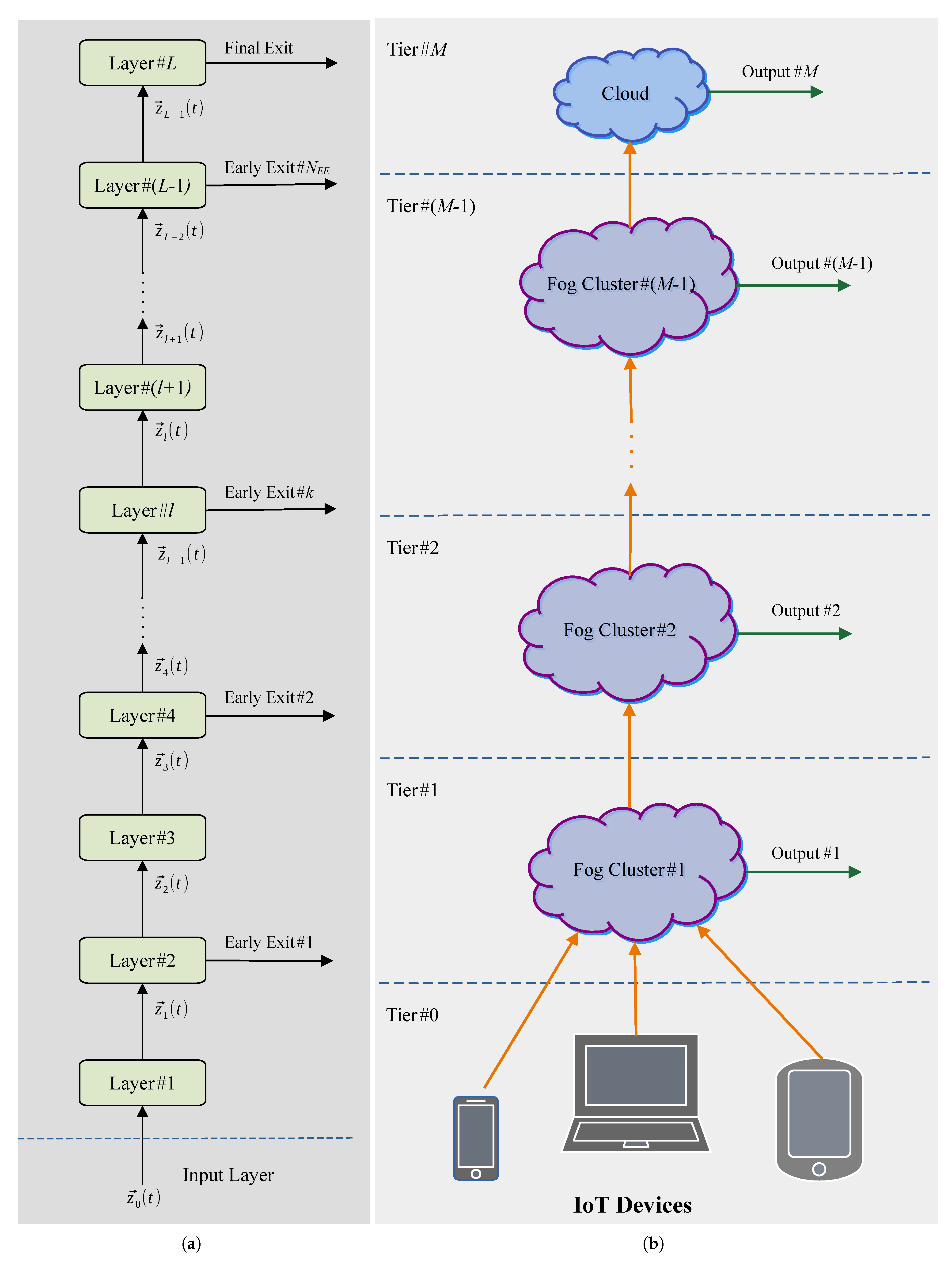
The emerging Deep Learning (DL) paradigm of the so-called Conditional Deep Neural Networks (CDNNs) with early exits [5,6,7], also known as BranchyNets [8,9], meets the first two requirements and provides an effective means of performing real-time analytics on structured/unstructured IoT data. As sketched in Figure 1a, a CDNN with early exits is obtained by augmenting the stack topology of a baseline feedforward Deep Neural Network (DNN) [10] with a number of local classifiers connected to associated intermediate output branches, called the early exits. The introduction of these auxiliary classifiers allows a fast prediction if there is enough confidence, i.e., the input data is sufficiently simple to be classified in the first layers, while more complicated data will use more or even all the CDNN layers, in order to provide reliable decisions. Both the reliability and associated delay of the local classifiers’ decisions increase, while moving from the bottom to the top of the CDNN stack. Hence, CDNNs with early exits may be capable of self-tuning the right reliability-vs.-delay tradeoff, so as to reduce both computing effort and inference delay, providing distributed local exit points to the running application.

In order to guarantee such a distributed implementation, the technological platform supporting the execution of a CDNN with early exits cannot rely only on a standing-alone remote and centralized cloud data center. It should be composed, indeed, of the networked interconnection of a number of hierarchically-organized computing nodes, which are spatially scattered and operate nearby the IoT devices. This is the native layout of the emerging paradigm of Fog Computing (FC) [11]. An FC technological platform (sketched in Figure 1b) enables pervasive local access to a set of $(M-1)$ clusters of virtualized small-size pools of computing resources, hierarchically-organized into tiers, which can be quickly provisioned, dynamically scaled up/down and released on an on-demand basis. Nearby resource-limited mobile devices may access these resources by establishing single-hop WiFi-supported communication links. The Fog paradigm exploits resource virtualization for supporting a set of virtualized services by distributing computing-plus-communication virtualized resources along the full path from the IoT realm to the remote Cloud data center [11] and offers a powerful paradigm for developing DL applications [12,13,14].

Interestingly enough, the IoT-CDNN-FC convergence can allow the exploitation of both the local exits of the implemented CDNNs and the per-tier aggregation of the local processing performed by the supporting FC platforms. In addition, this convergence may also allow the acquisition and joint mining of data generated by spatially scattered IoT device and may also enable energy and bandwidth-efficient data analytics by exploiting the scalable nature of the CDNNs and supporting FC platforms [11].

According to these facts, to enable an energy-efficient and real-time exploitation of the FC technological platform, we need a flexible evaluation environment for the dynamic test of different distribution strategies of CDNNs under programmable (i.e., settable by the user) models for the energy-delay profiles of the virtualized computing and network blocks composing the considered FC platform of Figure 1b.

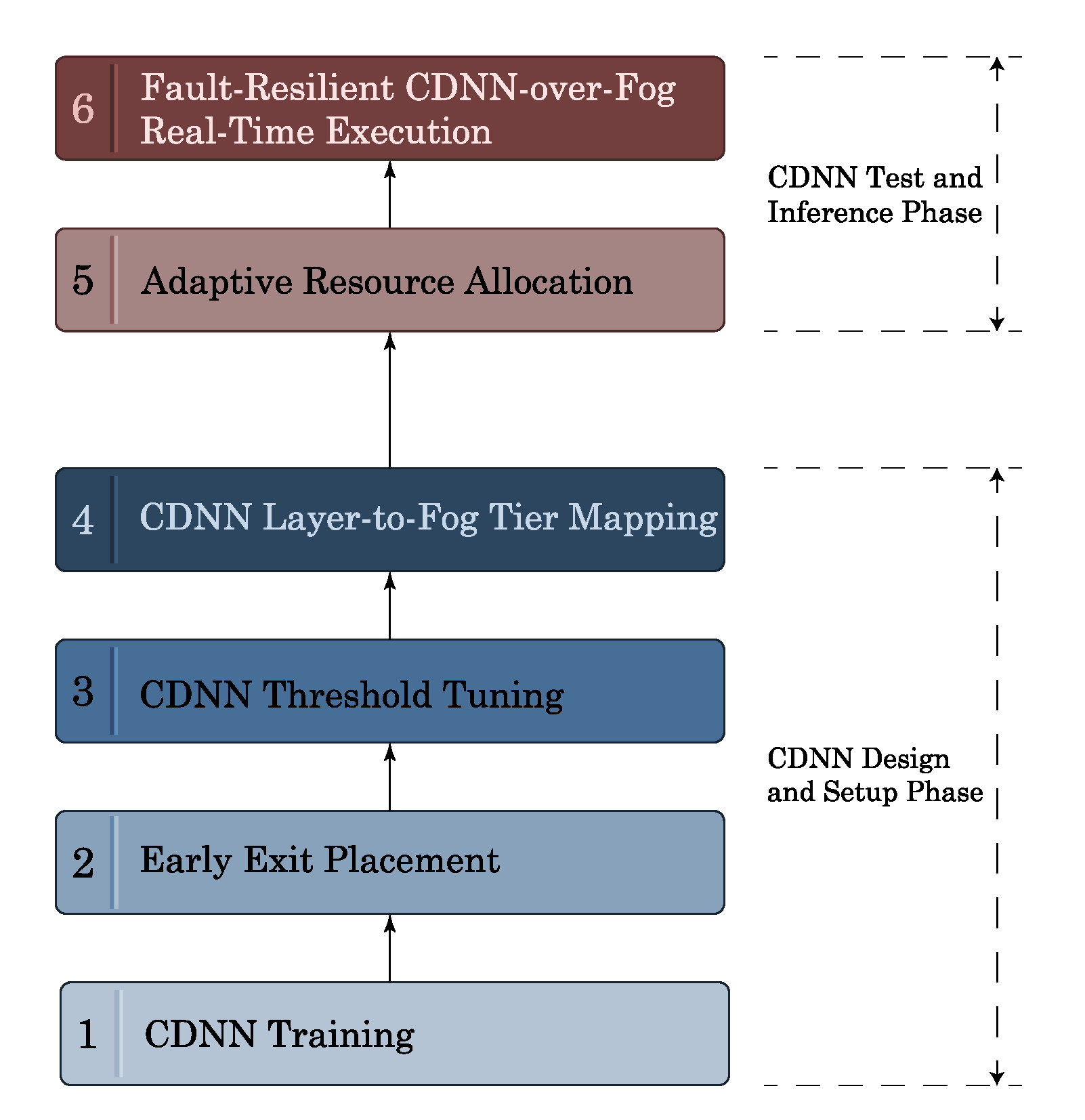
The steps to be taken for the design, training, and execution of the CDNN with early exits of Figure 1a over the distributed Fog technological platform of Figure 1b are sketched in Figure 2. The first four steps of Figure 2 concern the training/setup of the considered CDNN with early exits. All these steps have been the focus of our previous contributions in Reference [7,15], and will not be further considered in this paper. The last two steps of Figure 2 concern the inference phase of the CDNN’s life-cycle and will be the explicit focus of this contribution.

Motivated by these considerations, in this paper, we propose DeepFogSim, a toolkit supporting virtualized technological platforms for the real-time distributed execution of the inference phase of CDNNs with early exits under IoT realms.

In this perspective, DeepFogSim is a new software toolbox that allows:

• the simulation atop a standard PC;
• the dynamic optimization;
• the dynamic tracking;
• the comparison; and
• the graphic rendering through an ad-hoc designed Graphic Use Interface (GUI),

of the energy-vs.-delay performance of the underlying Fog-based technological platform supporting the execution of CDNNs with early exits. In particular, DeepFogSim tackles the joint CDNN inference and dynamic resource allocation problems, under hard real-time constraints on the overall (i.e., computing-plus-communication) execution time. Specifically, DeepFogSim allows the users to:

• test their desired network topologies by customizing the simulation environment through the setting of the 34 input parameters of the simulator package (see

  Table A2. Input parameters of the DeepFogSim simulator and their simulated settings of Section 7.

  Parameter	Meaning/Role	Measuring Units	Simulated Settings
  L	Number of the CDNN layers	Dimensionless	$L=9$
  $\overrightarrow{cm}$	Vector of per-layer compression	Dimensionless	$0<cm\left(m\right)\le 1$
  $T_S$	Duration of an inter-sensing period	(s)	$T_S=1$
  M	Number of tiers of the considered Fog platform	Dimensionless	$3\le M\le 6$
  ${\overrightarrow{pertier}}_{nodes}$	Vector collecting per-tier numbers of Fog nodes	Dimensionless	$1\le pertie{r}_{nodes}\left(m\right)\le 32$
  Q	Total number of Fog nodes	Dimensionless	$7\le Q\le 63$
  ${\overrightarrow{R}}^{\left(MAX\right)}$	Vector of maximum transport rate of each directed UDP/IP transport connection	(Mbit/s)	$8\le R^{\left(MAX\right)}\left(m\right)\le 9$
  ${\overrightarrow{v}}_0$	Vector of volumes of input data	(Mbit)	$1.5\le v_0\left(m\right)\le 1.5$
  $\left(A\right)$	Matrix describing the topology of the simulated multi-tier Fog platform	Dimensionless	Matrix entries in set $\left\{0,1\right\}$
  $\overrightarrow{\epsilon }$	Vector of per-node processing densities of convolutional processor	(CPU cycles/bit)	${10}^3\le \epsilon \left(m\right)\le 5\times {10}^3$
  $\overrightarrow{\beta }$	Vector of per-node processing densities of classifiers	(CPU cycles/bit)	$0.5\times {10}^3\le \beta \left(m\right)\le 2.5\times {10}^3$
  ${\overrightarrow{L2T}}_{map}$	Vector collecting the number of the CDNN layers that are mapped onto the m-th Fog tier, $m=1,\dots ,M$	Dimensionless	$1\le L2T_{map}\left(m\right)\le 4$
  ${\overrightarrow{T}}_{EXIT}$	Vector of the maximum tolerated delays for the per-tier local exits	(s)	$0.5\le T_{EXIT}\left(m\right)\le T_S$
  ${\overrightarrow{K}}_{CON}$	Vector of the scaling coefficients of the dynamic power consumed by the convolutional processors	(Watt/(CPU cycles/s)${}^{{\gamma }_{CON}}$)	$0\le K_{CON}\le 5\times {10}^{-36}$
  ${\overrightarrow{K}}_{CLA}$	Vector of the scaling coefficients of the dynamic power consumed by the classifier processors	(Watt/(CPU cycles/s)${}^{{\gamma }_{CLA}}$)	$0\le K_{CLA}\le 5\times {10}^{-36}$
  ${\overrightarrow{\gamma }}_{CON}$	Vector of the exponents of the dynamic power consumed by the convolutional processors	Dimensionless	$3\le {\gamma }_{CON}\left(m\right)\le 3.2$
  ${\overrightarrow{\gamma }}_{CLA}$	Vector of the exponents of the dynamic power consumed by the classifier processors	Dimensionless	$3\le {\gamma }_{CLA}\left(m\right)\le 3.2$
  ${\overrightarrow{P}}_{CON}^{\left(IDLE\right)}$	Vector of the idle power consumed by the convolutional processors	(Watt)	$P_{CON}^{\left(IDLE\right)}\left(m\right)={10}^{-7}$
  ${\overrightarrow{P}}_{CLA}^{\left(IDLE\right)}$	Vector of the idle power consumed by the classifier processors	(Watt)	$P_{CLA}^{\left(IDLE\right)}\left(m\right)={10}^{-7}$
  ${\overrightarrow{P}}_{NET}^{(IDLE;Rx)}$	Vector of the idle power consumed by each receive port	(Watt)	${10}^{-8}\le P_{NET}^{(IDLE;Rx)}\left(m\right)\le {10}^{-7}$
  ${\overrightarrow{P}}_{NET}^{(IDLE;Tx)}$	Vector of the idle power consumed by each transmit port	(Watt)	${10}^{-8}\le P_{NET}^{(IDLE;Tx)}\left(m\right)\le {10}^{-7}$
  $\overrightarrow{\psi }$	Vector of the dimensionless Transport-to-Physical protocol overheads at m-th tier	Dimensionless	$\psi \left(m\right)=1.105$
  ${\overrightarrow{\Omega }}_{NET}^{\left(Rx\right)}$	Vector of the scaling coefficients of the dynamic power consumed by each transmit port	(Watt/(bit/s)${}^{{\zeta }_{NET}^{\left(Tx\right)}}$)	$0\le {\Omega }_{NET}^{RX}\left(m\right)\le {10}^{-14}$
  ${\overrightarrow{\zeta }}_{NET}^{\left(Rx\right)}$	Vector of the exponents of the dynamic power consumed by each receive port	Dimensionless	$2.1\le {\zeta }_{NET}^{\left(Rx\right)}\left(m\right)\le 2.3$
  ${\overrightarrow{\Omega }}_{NET}^{\left(Tx\right)}$	Vector of the scaling coefficients of the dynamic power consumed by each transmit port	(Watt/(bit/s)${}^{{\zeta }_{NET}^{\left(Rx\right)}}$)	$0\le {\Omega }_{NET}^{RX}\left(m\right)\le {10}^{-14}$
  ${\overrightarrow{\zeta }}_{NET}^{\left(Tx\right)}$	Vector of the exponents of the dynamic power consumed by each transmit port	Dimensionless	$2.4\le {\zeta }_{NET}^{\left(Rx\right)}\left(m\right)\le 2.5$
  ${\overrightarrow{f}}^{\left(MAX\right)}$	Vector of the maximum processing frequencies of the convolutional processors	(Mbit/s)	$f^{\left(MAX\right)}\left(m\right)=9$
  ${\overrightarrow{\tilde{f}}}^{\left(MAX\right)}$	Vector of the maximum processing frequencies of the classifier processors	(Mbit/s)	${\tilde{f}}^{\left(MAX\right)}\left(m\right)=8$
  $I_{MAX}$	The maximum number of primal-dual iterations	Dimensionless	$I_{MAX}=450$
  $a_{MAX}$	Clipping factor of the step-sizes of the implemented primal-dual iterations	Dimensionless	$a_{MAX}=1.3\times {10}^{-5}$
  $iter\_number$	Total number of primal-dual iterations performed by each run of DynDeFog_TRACKER	Dimensionless	$iter\_number=450$
  ${\overrightarrow{a}}_{FogT}^{\left(MAX\right)}$	Vector of the clipping factors tested by each run of DynDeFog_TRACKER	Dimensionless	${10}^{-6}\le a_{FogT}^{\left(MAX\right)}\left(m\right)\le 7\times {10}^{-6}$
  ${\overrightarrow{jump}}_1$	Vector of the up/down multiplicative scaling factors applied to the scalar components of the input vectors of DynDeFog_TRACKER	Dimensionless	$0\le jum{p}_1\left(m\right)\le 1$
  ${\overrightarrow{jump}}_2$	Vector of the up/down multiplicative scaling factors applied to the scalar components of the input vectors of DynDeFog_TRACKER	Dimensionless	$0\le jum{p}_2\left(m\right)\le 1$

  );
• dynamically track the energy-delay network performance in the presence of abrupt (possibly, unpredictable) changes of the simulated environment, like mobility-induced changes of the available communication bandwidths; and
• optimize the obtained performance against a number of metrics, like total consumed energy, network consumed energy, network bandwidth, computing processing speeds, execution delays, just to name a few.

The major peculiar features of the proposed DeepFogSim toolbox are the following:

• it allows the numerical performance evaluation arising from the delay-constrained minimization of the overall computing-plus-network energy consumed by the execution of the CDNN with early exits. For this purpose, the DeepFogSim toolbox relies on a gradient-based primal-dual iterative procedure that implements a set of ad-hoc designed adaptive (i.e., time-varying) step-sizes;
• the resource allocation is performed by explicitly accounting for the virtualized nature of the utilized Fog platform;
• it allows the user to compare the energy-delay performance under a number of user-defined optimization strategies;
• it allows the display of the dynamic time-behavior of the performed resource allocation under the time-varying simulation environment set by the user; and
• it allows the rendering of the data output by the simulator in tabular, bar plot, and colored graph formats.

In this respect, we remark that the proposed DeepFogSim extends and complements our previous simulator VirtFogSim. Both these toolkits allow the dynamic joint optimization and tracking of the energy and delay performance of Mobile-Fog-Cloud systems. However, the VirtFogSim is designed for the execution of applications described by general Directed Application Graphs (DAGs), while the DeepFogSim aims at simulating the performance of CDNNs with early exits on a customizable networked Fog topology.

The rest of the paper is organized as follows. Section 2 overviews the literature about other simulation toolkits on Fog environment. Section 3 introduces the architecture of the main simulated building blocks, and, then, Section 4 describes the underlying optimization problem. Section 5 illustrates the general software architecture of the DeepFogSim toolkit, while Section 6 shows the supported formats for the rendered data. Section 7 presents several numerical results, and Section 8 concludes the work and provides some hints for future developments. Finally, the DeepFogSim user interface and the full list of all the parameters used by the simulator are described in Appendix A and Appendix B, respectively.

2. Related Work

Although the FC paradigm is a relatively recent field of research, there are already several tools for its software simulation [16,17,18]. This is because the most part of the current contributions constitute the follow-up of some toolkits designed for the simulation of the (more conventional) Cloud environment.

An overview of the current literature points out that the research on the development of simulation tools for Cloud-Fog computing platforms proceeded along three main research lines, i.e.,

• software for simulation of networked large-scale Cloud data centers;
• toolkits that explicitly account for the specific features of Fog platforms for the support of IoT-based sensor applications; and
• software toolkits for the simulation and performance evaluation of general multi-tier Cloud-Fog computing platforms.

Starting to overview the first more traditional research line, we point out that CloudSim [19] is a general-purpose simulation toolkit that allows modeling and simulation of applications atop remote Cloud platforms according to the Infrastructure-as-a-Service provisioning model. It allows the user to setup a customized modeling of the major building blocks of conventional Cloud infrastructures. However, it shows some deficiencies when applied to FC scenarios. Specifically, it does not allow the customized setup of network-related parameters (like the per-link wireless access bandwidths and the round-trip-times of Transport-layer TCP/IP connections), it relies only on Virtual Machine (VM)-based virtualization and does not allow the modeling of emerging Container (CNT)-based virtualization, the implemented resource allocation policies are of static-type and no support for dynamic resource tracking is provided. Similarly, the main focus of GreenCloud [20] is on the modeling and simulation of the energy profiles of some main computing and network components of the Cloud ecosystem. GreenCloud allows the customized setting and simulation of the full TCP/IP protocol stacks equipping the switches of the intra-cloud network, but it does not account for the Device-to-Cloud wireless links. Stemming from an extension of the traditional OMNeT++ platform, the iCanCloud [21] focuses on the simulation of Cloud-supported large ecosystems with thousands of served devices. Hence, being scalability the main concern of this toolkit, it does not support dynamic resource tracking and per-device performance optimization. Although based on the virtualization, these works, differently from the proposed one, do not explicitly consider Fog platforms.

About the second and more recent research line, we cite the SimIOT [22], which extends the (previously developed) SimIC [23] simulator by including a bottom IoT layer, in order to allow the user to model the request of Cloud resources by a settable number of sensor/actuator devices. Similarly, IOTSim [24] is implemented as an extension of the (aforementioned) CloudSim. Its goal is the simulation of FC environments in which sensor-acquired big data streams have to be quickly processed. For this purpose, the IOTSim platform is MapReduce-compliant, so that it implements batch processing models for the support of delay-tolerant big-data applications. iFogSim [25] is another JAVA-based toolbox in which implementation is an extension of CloudSim. It aims at simulating IoT-based Fog platforms by providing a set of suitable primitives for modeling the energy-delay performances of sensors, actuators, Fog and Cloud nodes, two service models and two heuristic task allocation policies. More recently, MyiFogSim [26] has extended the iFogSim simulator to support virtual machine migration policies for mobile users. Moreover, MobFogSim [27] has currently improved MyiFogSim by taking into account for the modeling of device mobility and service migration in FC. A different philosophy has been pursued by the EmuFog toolkit [28], which, instead of performing the simulation of large-scale topologies, generates networks that can be easily emulated by specific software designed for SDN (like MaxiNet, which extends the seminal Mininet emulation environment). Based on the OMNeT++ framework, the FogNetSim++ toolkit [29] allows simulation of a large Fog network with several user configurations. It also enables users to incorporate customized mobility models and FN scheduling algorithms so as to manage handover mechanisms. The goal of the Edge-Fog toolkit [30] is to distribute different processing tasks on the available Cloud resources. The assignment of the processing tasks to different cloud nodes is pursued by a customized cost function that jointly optimizes the processing time and networking costs. The Python-based simulator YAFS (Yet Another Fog Simulator) [31] aims at designing discrete-event Fog applications. It also allows the users to incorporate strategies for placement, scheduling and routing. The software toolkit EdgeCloudSim [32] is designed for the simulation and performance evaluation of general multi-tier Cloud-FC platforms. It provides the user with a software environment for the setting and dynamic simulation of the profiles of WLAN/WAN networks, wireless network traffic, device mobility, Fog nodes and Cloud nodes. A comprehensive comparative analysis between iFogSim, MyiFogSim, EdgeCloudSim, and YAFS simulators is provided in Reference [33]. In a similar manner, PureEdgeSim [34] allows the evaluation of the performance related to Cloud, Edge, and Mist computing environments by taking account of a number of resource management strategies. It shows a high scalability, since it is suitable for thousands of devices and it supports the devices heterogeneity. The toolkits of this second group consider distributed FC environments and resource management techniques. However, unlike the proposed work, they do not allow the dynamic tracking of the performed resource allocation under time-varying operating conditions and/or failure events affecting the underlying Fog execution platform.

Regarding the third research line, we start with the FogTorch toolkit [35]. It is a Java-based software simulator that allows the development of network models supporting the Quality of Service (QoS)-aware deployment of multicomponent IoT applications atop Fog infrastructures. The FogBus simulator [36] offers a platform independent interface to IoT applications. It also allows users to run multiple applications at a time and to manage network resources. In addition, FogBus takes care of security of sensitive data by applying Blockchain, authentication and encryption techniques. FogDirSim simulator [37] allows the user to analyze and compare different application management policies according to a set of user-defined performance indexes (like delay time, energy consumption, resource usage, etc.). It also allows us to model random resource fluctuations and infrastructure failures. FogWorkFlowSim [38] is a general-purpose toolkit that is developed to model and simulate the workflow scheduling in IoT, Edge, and FC environments. After the execution of the user submitted workflow, FogWorkFlowSim is capable of automatically evaluating and comparing the performance of different computation offloading and task scheduling strategies with respect to time delay, energy and cost performance. Our previous simulator, VirtFogSim [39], is a MATLAB-supported software toolbox that allows the dynamic joint optimization and tracking of the energy and delay performance of Mobile-Fog-Cloud systems for the execution of applications described by general Directed Application Graphs (DAGs). Specifically, it allows the joint dynamic energy-aware optimization of the placement of the application tasks and the allocation of the needed computing-networking resources under hard constraints on the allowed overall execution times, and it also allows the dynamic tracking of the performed resource allocation under time-varying operational environments. Although this group of toolkits tackles the joint optimization of energy and delay performance of IoT-Fog-Cloud environments, differently from DeepFogSim, they do not support the execution of CDNNs.

A summary of the mentioned simulators and their main targets is reported in

Table 1. Available toolkits for the simulation of Fog-based ecosystems.

Simulator	Main Target	Available at
CloudSim [19]	Allows the modeling and simulation of applications atop remote Cloud platform according to the IaaS model.	https://github.com/cloudslab/cloudsim
GreenCloud [20]	Offers a detailed fine-grained modeling of the energy consumed by data centers for Cloud applications.	https://greencloud.gforge.uni.lu/
iCanCloud [21]	Aims at modeling and simulating Cloud systems, in order to predict the trade-offs between cost and performance.	https://www.arcos.inf.uc3m.es/old/icancloud/Home.html
SimIOT [22]	Aims at modeling an inter-cloud facility wherein multiple clouds collaborate with each other for distributing service requests.	—
IOTSim [24]	Supports and enables simulation of IoT big data processing using MapReduce model in Cloud environments.	https://github.com/kalwasel/IoTSim-Osmosis
iFogSim [25]	Provides modeling and simulation tools for resource management techniques under IoT, Edge, and FC environments.	https://github.com/Cloudslab/iFogSim
MyiFogSim [26]	Extends the iFogSim simulator to support virtual machine migration policies for mobile users.	https://github.com/marciocomp/myifogsim
MobFogSim [27]	Extends iFogSim to enable modeling of device mobility and service migration in FC.	https://github.com/diogomg/MobFogSim
EmuFog [28]	Helps to generate networks that can be emulated by the MaxiNet software, a distributed version of the popular Mininet.	https://github.com/emufog/emufog
FogNetSim++ [29]	Simulates distributed FC environments by providing built-in modules to support the required communication protocols.	https://github.com/rtqayyum/fognetsimpp
Edge-Fog [30]	Generates a network of resources, supports task allocation, and configuration parameters.	https://github.com/nitindermohan/EdgeFogSimulator
YAFS [31]	Is a Python-based software to analyze FC ecosystems regarding the placement of resources, cost deployment, network design.	https://github.com/acsicuib/YAFS
EdgeCloudSim [32]	Provides a simulation environment for Edge Computing scenarios to experiment with both computational and networking resources.	https://github.com/CagataySonmez/EdgeCloudSim
PureEdgeSim [34]	Allows to evaluate the performance of resources management strategies in terms of network usage, latency, resources utilization, energy consumption.	https://github.com/CharafeddineMechalikh/PureEdgeSim
FogTorch [35]	Allows to develop models supporting the QoS-aware deployment of multicomponent IoT applications atop Fog infrastructures.	https://github.com/di-unipi-socc/FogTorch
FogBus [36]	Implements an end-to-end Edge-Cloud integrated environment for supporting users in running multiple applications at a time and service providers to manage their resources.	https://github.com/Cloudslab/FogBus
FogDirSim [37]	Permits to compare different application management policies and to consider random variations and failures of the underlying infrastructure.	https://github.com/di-unipi-socc/FogDirSim
FogWorkFlowSim [38]	Allows the performance evaluation of resource and task management strategies in FC under simulated user-defined workflow applications.	https://github.com/ISEC-AHU/FogWorkflowSim
VirtFogSim [39]	Allows the dynamic joint optimization and tracking of the energy and delay performance of Mobile-Fog-Cloud systems for the execution of applications described by DAGs.	https://github.com/mscarpiniti/VirtFogSim
DeepFogSim [Proposed]	Is the first tool for the simulation of the performance of the minimum-energy optimized execution of CDNNs with early exits over multi-tier networked distributed Fog platform under hard constraints on the allowed per-exit inference delays.	https://github.com/mscarpiniti/DeepFogSim

.

Overall, on the basis of the carried out review summarized in Table 1, the main new features of the proposed DeepFogSim toolkit are the following:

• DeepFogSim provides a software platform for the simulation of the energy-vs.-delay performance featuring the execution of CDNNs with early exits atop multi-tier distributed networked virtualized Fog technological platforms;
• DeepFogSim allows the user to explicitly model the joint effects on the resulting performance of the underlying Fog execution platform of both the fraction of the input data that undergoes early exits and the user-dictated constraints on the per-exit maximum tolerated inference delays; and
• DeepFogSim allows the dynamic tracking of the performed resource allocation under time-varying operating conditions and/or failure events affecting the underlying Fog execution platform.

This leads, indeed, to two main conclusions. First, the main pro of the proposed DeepFogSim toolkit is that it allows us to properly account for the impact of the multiple per-exit inference delays on the resulting minimum-energy allocation of the computing-plus-networking resources over the multi-tier Fog execution platform of Figure 1b. In this regard, we note that, to the best of our knowledge, up to date, there is no competing simulation toolbox which natively retains this feature, and the synoptic overview of the related work of Table 1 supports, indeed, this conclusion. Second, a possible limitation of the current version of the DeepFogSim toolkit may arise from the fact that the implemented optimization engine inherently exploits the hierarchically-organized stack topology featuring the overall family of the here considered feedforward DNNs (see Figure 1a). This precludes, indeed, the application of the proposed toolkit for the simulation of the inference phase of neural networks which do not retain stacked-type topologies, such as, for example, the family of the so-called Recurrent Neural Networks (RNNs) [10].

We finally remark that, by design, the DeepFogSim toolkit refers to the simulation of the inference phase of the CDNN with early exits of Figure 1a over the multi-tier Fog execution platform of Figure 1b. Hence, topics related to: (i) the optimized design and placement of the CDNN early exits; (ii) the CDNN training; and (iii) the optimized mapping of the CDNN layers of Figure 3 onto the Fog tiers of Figure 1b are not the focus of this paper. All these topics have been afforded in our previous contribution in Reference [15].

3. The Envisioned Fog Computing Architecture Supporting the CDNN Execution

In order to describe more in depth the FC platform and the application that should run atop it, we assume that a data vector ${\overrightarrow{z}}_0\left(t\right)$, arriving at the input of the CDNN of Figure 1a at time t, is processed in a layer-wise way, moving from $layer\#1$, in order to generate a local class label (i.e., a local decision). If the confidence level computed by the local classifier at $layer\#l$, $1\le l\le L-1$, is high enough, the processing is stopped and a decision is output from the l-th branch of Figure 1a. In the opposite case, the feature vector ${\overrightarrow{z}}_l\left(t\right)$ extracted by $layer\#l$ is passed to the next $layer\#(l+1)$ for further processing. Only when an input data is so challenging to classify to require the processing by the full CDNN stack that the corresponding decision is generated by the last L-th layer, irrespective of its actual confidence level.

3.1. On the Hierarchical Organization of the FC Technological Platform

As stated in Section 1, the FC platform is suitable to execute CDNNs with early exits. The resulting FC technological platform is typically composed of a set of $(M-1)$ clusters of medium-size virtualized data centers (i.e., Fog Nodes (FNs)), which are hierarchically-organized into tiers and exploit (typically wireless) transport links for enabling inter-tier communication. Doing so, a communication path is implemented from the lowermost IoT realm at $tier\#0$ to the uppermost Cloud Node (CN) at $tier\#M$. At each intermediate $tier\#m$, with $1\le m\le M-1$, an intra-tier local network allows an AGgregator (AG) node to provide an early exit by suitably merging the outputs of the corresponding FNs into a local output (see the per-tier side branches in Figure 1b). Doing so, it is expected that only a small fraction of the volume $v_0\left(t\right)$ of data generated by the IoT devices at time t needs to be transported up to the remote CN for analytics, while a (hopefully) large part of $v_0\left(t\right)$ early exits through the available intermediate per-tier local outputs. Figure 3 shows a sketch of the envisioned multi-tier networked technological platform for the distributed execution of the inference phase of an (already designed and trained) CDNN with early exits.

Basically, the Fog platform of Figure 3 is composed of the hierarchically organized cascade of three main segments, namely:

• the lowermost segment (i.e., $tier\#0$), where a set of spatially distributed resource-poor IoT sensors operate. Since current IoT devices (for example, smartphone, tablets and personal assistants, just to name a few) are natively equipped with built-in sensors, IoT devices at $tier\#0$ are assumed to be co-located with Fog nodes at $tier\#1$ (see the dark blue triangles at the bottom of Figure 3);
• the middle segment, where a number of spatially distributed and networked Fog nodes operates. According to Figure 3, this segment is hierarchically organized into $(M-1)$ stacked tiers numbered from $tier\#1$ to $tier\#(M-1)$. At $tier\#m$, with $1\le m\le M-1$, a cluster: $\{\mathrm{Fog}(j,m),1\le j\le m_m\}$, with $m_m\ge 1$, of Fog nodes operates by exchanging data with a local aggregator $AG\left(m\right)$ over an intra-tier LAN. From time to time, the local $Detector\#m$ generates a local decision ${\widehat{c}}_m$ (i.e., a class label) on the current input data generated by the sensors at $tier\#0$ when the confidence level of the per-tier aggregated data ${\overrightarrow{\widehat{Y}}}_m$ delivered by $AG\left(m\right)$ is high enough (see the dotted red lines in Figure 3). In the opposite case (i.e., when the confidence level of ${\overrightarrow{\widehat{Y}}}_m$ is estimated to not be high enough), the local output is the empty set: ∅, that is, no data is generated by the m-th local output;
• the uppermost segment (i.e., $tier\#M$), where a (single) remote Cloud node (labeled as Fog$(1,M)$ in Figure 3) operates. Its task is to perform complex analytics on the most hard-to-classify input instances, so as to provide a final decision ${\widehat{c}}_M$ on the class label of the currently sensed input data, regardless of its actual confidence level.

From time to time, the sensors at the bottom of the technological platform of Figure 3 sense the local surrounding environment and then pass the sensed data in upstream for its tier-by-tier hierarchical mining. At each intermediate $tier\#m$, with $1\le m\le (M-1)$, an (average) fraction ${\rho }_m$ of the input data is passed to the next $tier\#(m+1)$ for further processing, while the remaining fraction $(1-{\rho }_m)$ undergoes local exit, in order to produce the corresponding decision ${\widehat{c}}_m$. Due to the real-time nature of the considered IoT application scenario, the inference-delay, at which the decision ${\widehat{c}}_m$ exits at each $tier\#m$, $1\le m\le M$, is assumed to be limited up to a per-tier upper bound $T_{EXIT}^{\left(m\right)}$ (s), $1\le m\le M$, in which the actual value is set on the basis of the Quality of Service (QoS) requirements of the supported application.

In order to support real-time inference, the time axis, over which the platform of Figure 3 operates, is partitioned into time-slots which are labeled by a discrete-time slot-index $t\ge 0$. In the case of periodic sensing, the slot duration is fixed at $T_S$, so that the t-th slot spans the half-open time-interval: $(t{T}_S,(t+1)T_S)$. In the more general case of event-driven sensing, the duration ${\Delta }_S\left(t\right)$ of the t-th slot depends on the slot-index t, so that the t-th slot covers the half-open interval: $(\xi \left(t\right),\xi \left(t\right)+{\Delta }_S\left(t\right))$, where: $\xi \left(t\right)\triangleq {\sum }_{i=0}^{t-1}{\Delta }_S\left(i\right)$ is the starting time of the t-th slot. We expect that all the results presented in the following hold verbatim in both cases of periodic and event-driven sensing, provided that, in the second case, the minimum slot duration is lower bounded by $T_S$, that is, ${\Delta }_S\left(t\right)\ge T_S$, $\forall t$.

The envisioned technological platform of Figure 3 is assumed to be equipped with both networking and computing capabilities. Specifically, the required inter-node message passing is implemented by a number of inter-tier and intra-tier transport connections (see the arrows of Figure 3). Up-link communication between FNs falling in adjacent tiers is supported by a number of TCP/IP one-way reliable connections, which are sustained by wireless (possibly, single-hop and WiFi-based) communication links (see the continuous purple arrows in Figure 3 between adjacent tiers). Since load balancing is assumed to be performed at the outputs of each tier, all the transport connections going from Fog nodes at $tier\#m$ to Fog nodes at $tier\#(m+1)$ are assumed to operate at a same bit-rate of $R_m$ (bit/s). Horizontal communication between the Fog nodes and the Aggregator falling into the same tier is assured by an intra-tier (wired or wireless) LAN which relies on UDP/IP two-way transport connections (see the continuous blue arrows in Figure 3). Being of local-type and used only for (sporadic) aggregation operations, these intra-tier connections are assumed to operate at low bit-rates, so that the impact of their energy consumption is expected not to be so substantial.

Finally, the protocol stack implemented by the envisioned architecture of Figure 3 is detailed in Figure 4. Specifically, the three-layered architecture of the simulated protocol stack of Figure 4 reflects the corresponding partition of the technological platform of Figure 3 into three hierarchically-organized main segments, namely: (i) the lower-most segment, at which the IoT devices operate; (ii) the middle segment, which embraces the clusters of Fog nodes; and (iii) the upper-most segment, where the remote Cloud works.

Remark—On the optimality of the considered multi-tier hierarchically-organized Fog topology. A final remark concerns the generality and optimality of the considered hierarchically-organized and multi-tier Fog topology of Figure 1b and Figure 3. In this regard, four main considerations are in order. First, due to its feedforward nature, the topology in Figure 1a of the CDNN to be executed is, by design, of stack-type. This forces, in turn, to select a hierarchically-organized companion topology for the corresponding execution platform of Figure 1b, in order to allow the ordered execution of the layers of the supported CDNN. Second, the multi-tier feature of the considered Fog platform of Figure 1b and Figure 3 is dictated by the requirement that the execution of the inference phase of the CDNN of Figure 1a can be of distributed-type. Third, the Fog execution platform sketched in Figure 3 allows, by design, that: (i) the number M of the Fog tiers; (ii) the number $m_m$ of the Fog nodes equipping the m-th tier; (iii) the topologies of the inter-tier networks of Figure 3; and (iv) the number and placement of the output local branches of Figure 3 are freely set and customized by the designer on the basis of the actually considered application scenarios. Overall, these considerations support the conclusion that the considered networked Fog topology of Figure 3 suitably matches the main requirements demanded for the distributed execution of the inference phase of the overall family of the feedforward CDNNs with early exits of Figure 1a.

3.2. On the Optimized Layer-to-Tier Mapping

A factor impacting on the energy consumed by the execution of the inference phase of the CDNN of Figure 1a on the distributed multi-tier networked computing platform of Figure 1b is the adopted strategy for mapping the CDNN layers onto the available Fog/Cloud tiers. This problem has been afforded in deep in our recent contribution in Reference [15]. Hence, here we only recap the main results.

Therefore, according to Reference [15], let us consider a partition ${\mathcal{T}}_m\subseteq \left\{1,2,\dots ,L\right\}$, $m=1,\dots ,M$, of the set of the layers of the CDNN of Figure 1a into M subsets, which is characterized by the following three defining properties:

• the first (respectively, last) layer of the CDNN of Figure 1a is mapped onto an element of the set ${\mathcal{T}}_1$ (respectively, ${\mathcal{T}}_M$) of the considered partition;
• the $\left|{\mathcal{T}}_m\right|$ elements of ${\mathcal{T}}_m$ are the indexes of consecutive (that is, adjacent) CDNN layers;
• the cluster of computing nodes at $tier\#m$, $1\le m\le M$, exhibits sufficient computing power and communication bandwidth to host all the layers of the m-th partition set ${\mathcal{T}}_m$.

In Reference [15], it was formally proved that, at least in the case in which all the involved computing nodes exhibit the same power-consumption profile, such a kind of partition individuates a feasible Layer-to-Tier mapping ${\mathcal{T}}_m$, which minimizes the average energy wasted by the multi-tier platform of Figure 1b for the execution of the CDNN of Figure 1a. Motivated by this formal result, we assume that the mapping of the layers of the CDNN of Figure 1a onto the tiers of the execution platform of Figure 1b has been already performed according to this minimum-energy criterion.

4. DeepFogSim: The Considered System Model

In this section, we introduce the basic definitions and formal assumptions about the constrained resource optimization problem tackled by the DeepFogSim.

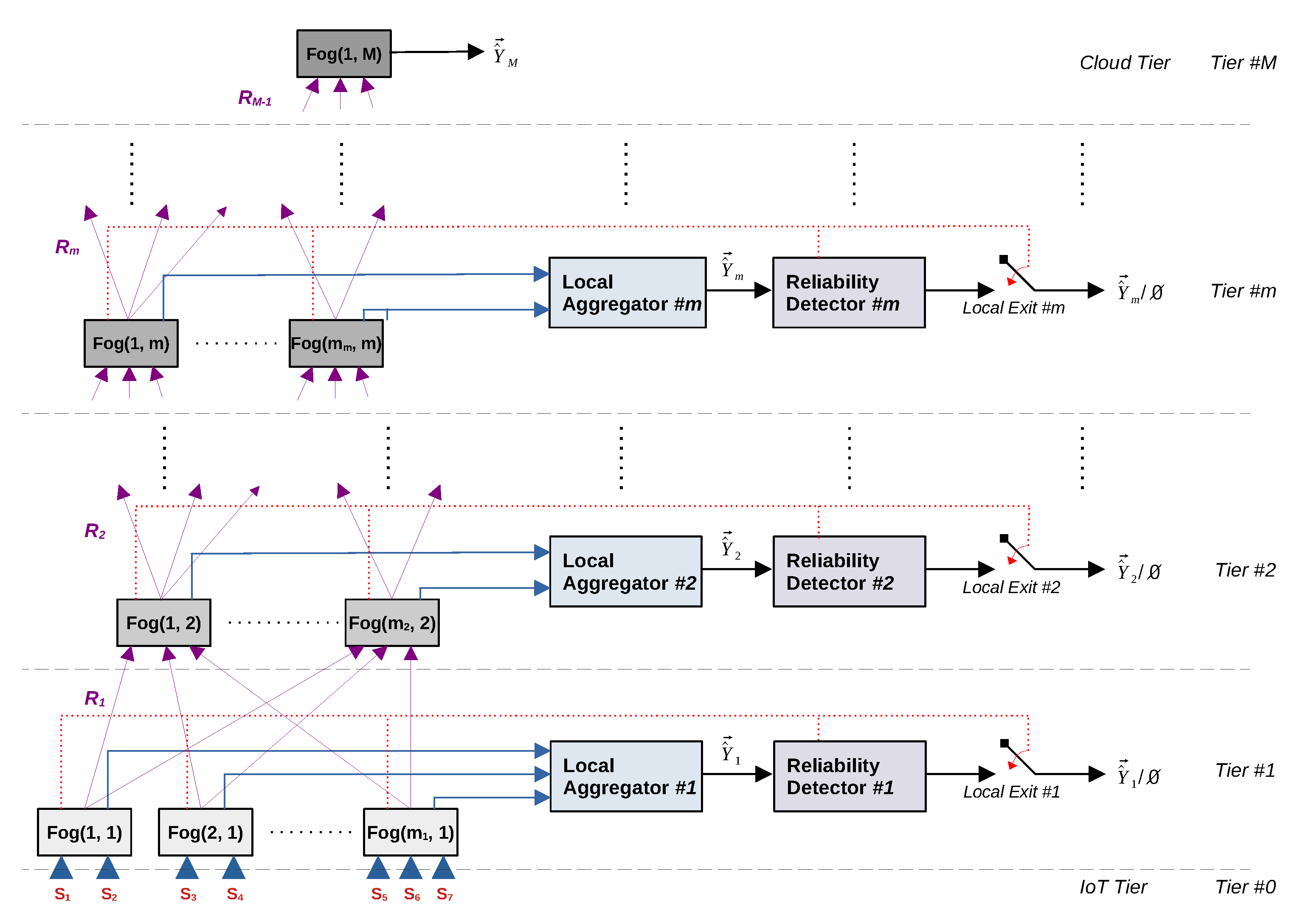
For this purpose, let us denote by Fog$(j,m)$ the j-th FN located at $tier\#m$, with $j=1,\dots ,m_m$ and $m=1,\dots ,M$, where $m_m$ is the total number of FNs present in the m-th tier, while M is the total number of tiers. By definition, the last M-th tier is the Cloud one. Moreover, let us denote by ${\overrightarrow{z}}_0\left(t\right)$ the data vector arriving at the input of the CDNN of Figure 3 at time t that will be processed in a layer-wise way, moving from $layer\#1$. In a similar way, we denote by ${\overrightarrow{z}}_l\left(t\right)$ the feature vector extracted by $layer\#l$ and passed to the next $layer\#(l+1)$ for further processing.

4.1. Container-Based Virtualized Fog Node Architecture

In principle, the technological platform of Figure 3 may run, in parallel, multiple CDNNs which carry out different analytics on the same set of sensed data by resorting to the virtualization of the full spectrum of available physical resources [40].

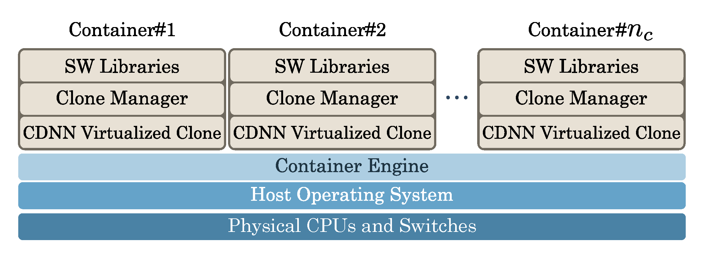
Hence, according to this consideration, we assume that all Fog/Cloud nodes of Figure 3 are equipped with software clones of the run CDNNs. The number of clones simultaneously hosted by each FN equates to the number of (possibly, multiple) CDNNs which are running in parallel over the technological platform of Figure 3. Doing so, each clone is fully dedicated to the execution of a single associated CDNN, and then it acts as a virtual “server” by providing resource augmentation to the tied “client” CDNN. For this purpose, each clone is executed by a container (CNT) that is instantiated atop the hosting FN. The container is capable of using (through resource multiplexing) a slice of the physical computing and networking resources of the hosting FN. The logical view of the resulting virtualized container-based FN is detailed in Figure 5.

All containers hosted by Fog$(j,m)$ in Figure 5 share: (i) a same Host Operating System (HOS); and (ii) the pool of computing (i.e., CPU cycles) and networking (i.e., bandwidth and I/O Network Interface Cards (NICs) and switches) physical resources available on the hosting FN. The task of the Container Engine of Figure 5 is to allocate these physical resources to the requiring containers by performing dynamical multiplexing.

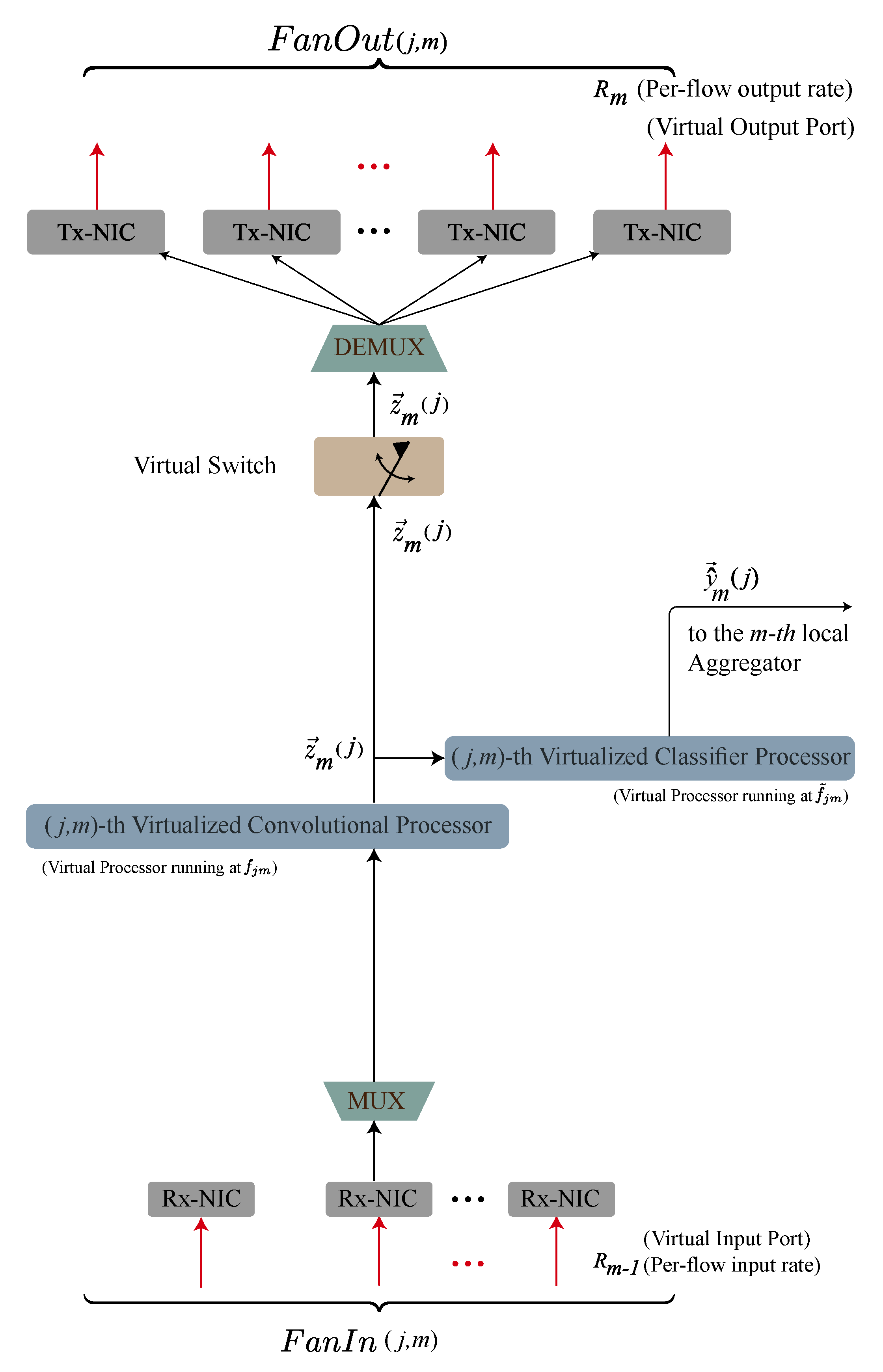
The resulting virtualized architecture of Fog$(j,m)$ is sketched in Figure 6. Specifically, in Figure 6 we have that:

• the $(j,m)$-th Virtualized Convolutional Processor, running at frequency $f_{jm}$, provides the computing support for the execution of the set of $\left|{\mathcal{T}}_m\right|$ consecutive convolutional and pooling layers of the supported CDNN to be executed on $tier\#m$. In the envisioned architecture, the input data ${\overrightarrow{z}}_{m-1}\left(j\right)$ at the Virtualized Convolutional Processor is a feature vector received from the FNs working at the previous $tier\#(m-1)$, while the corresponding output data ${\overrightarrow{z}}_m\left(j\right)$ is provided to the associated Virtualized Classifier Processor, as well as forwarded to the FNs operating at the next $tier\#(m+1)$;
• the $(j,m)$-th Virtualized Classifier Processor, running at frequency ${\tilde{f}}_{jm}$, provides the computing support for the execution of the local classifier of the CDNN. Its task is to process the feature vector generated by the corresponding Virtualized Convolutional Processor, so as to produce the output vector ${\overrightarrow{\widehat{y}}}_m\left(j\right)$ to be delivered to the corresponding m-th Local Aggregator of Figure 3 for the (possible) generation of an early-exit;
• Fog$(j,m)$ is also equipped with a number $FanIn(j,m)\ge 1$ of virtualized input ports. Hence, the task of the MUltipleXer (MUX) at the bottom of Figure 6 is to merge the corresponding information flows received by the FNs operating at the previous $tier\#(m-1)$, so as to generate a (single) aggregate feature vector ${\overrightarrow{z}}_{m-1}\left(j\right)$. All input flows at the bottom of Figure 6 are assumed to operate at a same bit-rate $R_{m-1}$ (bit/s);
• the main task of the De-MUltipleXer (DEMUX) at the top of Figure 6 is to replicate the received feature vector ${\overrightarrow{z}}_m\left(j\right)$ over the $FanOut(j,m)\ge 1$ virtualized output ports equipping Fog$(j,m)$. Each output flow is forwarded to the FNs at the next $tier\#(m+1)$ at a bit-rate $R_m$ (bit/s); and
• the task of the Virtual Switch (VS) of Figure 6 is to enable the transmission of the output feature ${\overrightarrow{z}}_m\left(j\right)$ to the FNs at the next $tier\#(m+1)$ only when early-exit does not occur at $tier\#m$.

4.2. Featuring the Average Traffic and Workload

Since all FNs of a same tier of Figure 3 cooperate, by definition, in performing the same type of processing, all flows output by FNs of $tier\#m$ have the same throughput $R_m$ (bit/s), with $1\le m\le M-1$.

In the case that $\left|{\mathcal{T}}_m\right|$ consecutive layers of the supported CDNN collapse into a single component layer at the m-th tier, the corresponding layer interior architecture becomes composed of the cascade of $\left|{\mathcal{T}}_m\right|$ convolutional blocks followed by a single nonlinearity and a single soft-decisor that sits atop the last convolutional blocks. As a consequence of these architecture features, we have that:

• the processing density of each $(j,m)$-th Fog convolutional processor passes from ${\epsilon }_m$ to $\left|{\mathcal{T}}_m\right|{\epsilon }_m$;
• the processing density of each $(j,m)$-th Fog classifier processor is ${\beta }_m$, regardless of the number $\left|{\mathcal{T}}_m\right|$ of CDNN layers, which are executed by the FNs at $tier\#m$;
• the average volume of data $v_I(j,m)$ (bit) received in input by Fog$(j,m)$ during each sensing period is:

  $$v_I(j,m)\triangleq E\left\{dim\left({\overrightarrow{z}}_{m-1}\left(j\right)\right)\right\}=v_0\times \left(\prod _{k=1}^{{\sum }_{j=1}^{m-1}\left|{\mathcal{T}}_j\right|}c{m}_k\right)\times \frac{FanIn(j,m)}{{\sum }_{\tau =1}^{m_m}FanIn(\tau ,m)},$$

  (1)

  where $E\left\{·\right\}$ denotes the expectation and $dim\left(\overrightarrow{z}\right)$ is the size (in bit) of the vector $\overrightarrow{z}$;
• the average volume of data $v_O(j,m)$ (bit) output by Fog$(j,m)$ is:

  $$v_O(j,m)\triangleq E\left\{dim\left({\overrightarrow{z}}_m\left(j\right)\right)\right\}=v_0\times \left(\prod _{k=1}^{{\sum }_{j=1}^m\left|{\mathcal{T}}_j\right|}c{m}_k\right)\times \frac{FanIn(j,m)}{{\sum }_{\tau =1}^{m_m}FanIn(\tau ,m)}.$$

  (2)

4.3. Per-Node Execution Times

Since we assume that the transmit Network Interface Cards (NICs) of Fog$(j,m)$, at the top of Figure 6, may operate in parallel, the per-node execution time $T_{EXE}(j,m)$ can be expressed as the summation of three terms, i.e., the computation time $T_{CON}(j,m)$, the classification time $T_{CLA}(j,m)$ and the network transmission time $T_{NET}(j,m)$. Hence, it equates:

$$T_{EXE}(j,m)\triangleq T_{CON}(j,m)+T_{CLA}(j,m)+T_{NET}(j,m)\equiv \frac{v_I(j,m)}{f_{j,m}}+\frac{v_O(j,m)}{{\tilde{f}}_{j,m}}+\frac{v_I(j,m)}{R_m},$$

(3)

where $f_{jm}$ (respectively, ${\tilde{f}}_{jm}$) is the processing speed (in (bit/s)) of the convolutional processor (respectively, the classifier processor) equipping Fog$(j,m)$ (see Figure 6).

Furthermore, since the Cloud does not perform transmission but only convolutional and classify tasks, its execution time comprises only the first two terms of the above expression, that is:

$$T_{EXE}(1,M)\triangleq T_{EXE}^{\left(Cloud\right)}\equiv \frac{v_I(1,M)}{f_{1,M}}+\frac{v_O(1,M)}{{\tilde{f}}_{1,M}}.$$

(4)

4.4. Per-Tier Execution Times

Since the m-th local aggregator in Figure 3 must receive all the $\left|\mathcal{Q}\right|$-dimensional vectors $\left\{{\overrightarrow{y}}_j\left(m\right)\in {[0,1]}^{\left|\mathcal{Q}\right|},1\le j\le m_m\right\}$ before performing its final operation, the (per-tier) execution time $T_{EXE}\left(m\right)$ at $tier\#m$ equates to the execution time of the slowest FN, so that we have:

$$T_{EXE}\left(m\right)\equiv \underset{1\le j\le m_m}{max}\left\{T_{EXE}(j,m)\right\}.$$

(5)

By definition, the multi-tier Fog architecture of Figure 3 processes the data generated by IoT devices of Figure 3 in a sequential way. Hence, the aggregate execution time $T_{EXE}^{(1,m)}$ needed to generate the local exit at $tier\#m$ equates to:

$$T_{EXE}^{(1,m)}=\sum _{k=1}^m{T}_{EXE}\left(k\right)\equiv \sum _{k=1}^m\underset{1\le j\le m_k}{max}\left\{T_{EXE}(j,k)\right\},1\le m\le M,$$

(6)

so that the resulting time constraint on the allowed local decision at $tier\#m$ reads as follows:

$$T_{EXE}^{(1,m)}\le T_{EXIT}^{\left(m\right)},1\le m\le M,$$

(7)

where $T_{EXIT}^{\left(m\right)}$ is the tolerated upper bound on the time needed for the generation of the local decision at $tier\#m$.

4.5. Models of the Per-Node Computing Power and Energy

In this subsection, we provide the formal relationships modeling the power and energy consumption of each FN. Specifically, we analyze separately the contributions of the convolutional and classifier processors equipping each FN in Figure 6.

4.5.1. Power and Energy Wasted by the Convolutional Processor

The power wasted by the convolutional processor of Fog$(j,m)$ in Figure 6 is composed of a static part ${\mathcal{P}}_{CON}^{\left(IDLE\right)}(j,m)$ (Watt), with $1\le j\le m_m$ and $1\le m\le M$, and a dynamic one:

$${\mathcal{P}}_{CON}^{\left(DYN\right)}(j,m)=K_{CON}^{(j,m)}{\left(\left|{\mathcal{T}}_m\right|{\epsilon }_{jm}{f}_{ij}\right)}^{{\gamma }_{CON}^{(j,m)}},1\le j\le m_m,1\le m\le M,$$

(8)

where [41]:

• ${\gamma }_{CON}^{(j,m)}$ is a dimensionless power exponent that depends on the power profile of the underlying CPU;
• ${\epsilon }_{jm}$ (CPU cycle/bit) is the so called processing density of the computation operations performed by the underlying CPU when a single layer of the CDNN must be executed. It depends on the number of convolutional neurons that compose a single layer of the considered CDNN and the average number of summations/multiplications performed by each neuron [15];
• $f_{jm}$ (bit/s) is the processing frequency of the $(j,m)$-th convolutional processor;
• $\left|{\mathcal{T}}_m\right|$ is the number of layers of the underlying CDNN to be executed by Fog$(j,m)$. This term accounts for the fact that the workload to be processed by the $(j,m)$-th convolutional processor scales (more or less) linearly with the number $\left|{\mathcal{T}}_m\right|$ of convolutional layers of CDNN to be executed by the Fog$(j,m)$ [15]; and
• $K_{CON}^{(j,m)}$, measured in (Watt/(CPU cycle/s)${}^{{\gamma }_{CON}^{(j,m)}}$), is a power scaling factor that depends on the power profile of the CPU supporting the $(j,m)$-th convolutional processor.

In order to compute the (average) energy ${\mathcal{E}}_{CON}^{(j,m)}$ (Joule) consumed by the $(j,m)$-th convoultional processor during each sensing interval, we note that: (i) the $(j,m)$-th convolutional processor must remain turned ON for a time $T_{EXE}^{(1,M)}$ equal to the execution time required by the Cloud node of Figure 3, i.e., the maximum time needed for the processing of the data generated by the server in a sensing period; and (ii) since the $(j,m)$-th convolutional processor works at the processing speed $f_{jm}$ (bit/s) and the workload to be executed is $v_I(j,m)$ in (1), the resulting processing time is $T_{CON}(j,m)$ in (3). Hence, we have the following relationship for ${\mathcal{E}}_{CON}(j,m)$:

$$\begin{array}{cc}\hfill {\mathcal{E}}_{CON}(j,m)& \triangleq {\mathcal{E}}_{CON}^{\left(IDLE\right)}(j,m)+{\mathcal{E}}_{CON}^{\left(DYN\right)}(j,m)\equiv {\mathcal{P}}_{CON}^{\left(IDLE\right)}(j,m)\times T_{EXE}^{(1,M)}+{\mathcal{P}}_{CON}^{\left(DYN\right)}(j,m)\times T_{CON}(j,m)\hfill \\ \hfill & ={\mathcal{P}}_{CON}^{\left(IDLE\right)}(j,m)\times T_{EXE}^{(1,M)}+v_I(j,m)K_{CON}^{(j,m)}{\left(\left|{\mathcal{T}}_m\right|{\epsilon }_{jm}\right)}^{{\gamma }_{CON}^{(j,m)}}\times f_{ij}^{{\gamma }_{CON}^{(j,m)}-1},\hfill \end{array}$$

(9)

where $T_{EXE}^{(1,M)}\equiv {\sum }_{k=1}^M{max}_{1\le j\le m_k}\left\{T_{EXE}(j,k)\right\}$ is the full (i.e, worst case) execution time of the supported CDNN of Figure 1a.

4.5.2. Power and Energy Wasted by the Classifying Processor

Let ${\mathcal{P}}_{CLA}^{\left(IDLE\right)}(j,m)$ (Watt) be the idle power consumed by the CPU of the $(j,m)$-th classifying processor in Figure 6. Then, the corresponding dynamic power component may be modeled as [41]:

$${\mathcal{P}}_{CLA}^{\left(DYN\right)}(j,m)=K_{CLA}^{(j,m)}{\left({\beta }_{jm}{\tilde{f}}_{jm}\right)}^{{\gamma }_{CLA}^{(j,m)}},1\le j\le m_m,1\le m\le M,$$

(10)

where:

• ${\gamma }_{CLA}^{(j,m)}$ is a dimensionless power exponent that depend on the power profile of the underlying CPU;
• ${\tilde{f}}_{jm}$ (bit/s) is the processing frequency of the $(j,m)$-th classifying processor;
• ${\beta }_{jm}$ (CPU cycle/bit) is the processing density of the computation operations performed by the underlying CPU [15]; and
• $K_{CLA}^{(j,m)}$, measured in (Watt/(CPU cycle/s)${}^{{\gamma }_{CLA}^{(j,m)}}$), is a positive scaling factor that depends on the power consumption of the CPU that supports the $(j,m)$-th classifier.

Hence, the energy ${\mathcal{E}}_{CLA}(j,m)$ (Joule) consumed by the $(j,m)$-th classifier during a sensing interval equates to:

$$\begin{array}{cc}\hfill {\mathcal{E}}_{CLA}(j,m)& \triangleq {\mathcal{E}}_{CLA}^{\left(IDLE\right)}(j,m)+{\mathcal{E}}_{CLA}^{\left(DYN\right)}(j,m)\equiv {\mathcal{P}}_{CLA}^{\left(IDLE\right)}(j,m)\times T_{EXE}^{(1,M)}+{\mathcal{P}}_{CLA}^{\left(DYN\right)}(j,m)\times T_{CLA}(j,m)\hfill \\ \hfill & ={\mathcal{P}}_{CLA}^{\left(IDLE\right)}(j,m)\times T_{EXE}^{(1,M)}+v_O(j,m)K_{CLA}^{(j,m)}\times {\left({\beta }_{jm}\right)}^{{\gamma }_{CLA}^{(j,m)}}\times {\left(f_{ij}\right)}^{{\gamma }_{CLA}^{(j,m)}-1},\hfill \end{array}$$

(11)

with $T_{EXE}^{(1,M)}$ being still the full (i.e, worst case) execution time.

4.6. Models of the Per-Flow Networking Power and Energy

Before developing the power/energy network models, some remarks about the network aspects of the Fog platform of Figure 3 are in order.

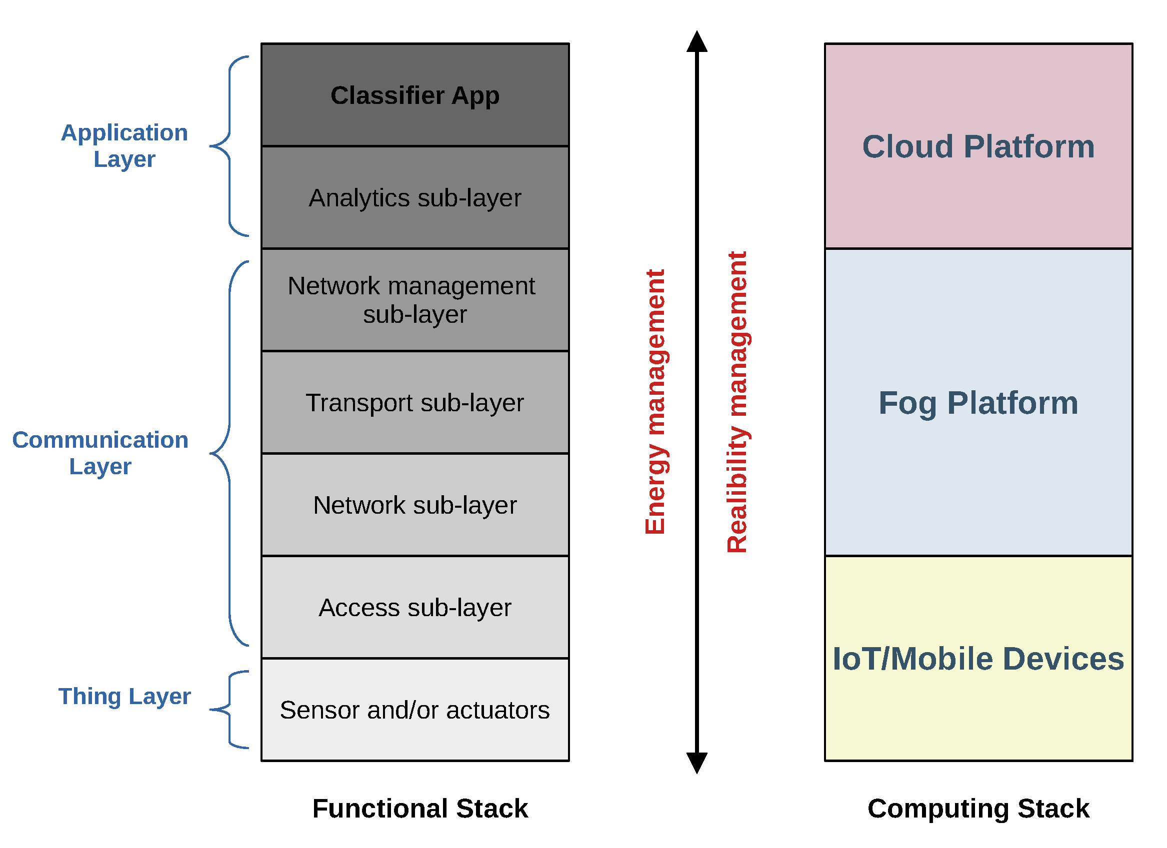
First, we assume that the m-th bit-rate $R_m$ (bit/s), $1\le m\le M-1$ in Figure 3 is a per-flow transport-layer throughput. However, both the consumed network power and energy depend on the corresponding bit-rate ${\widehat{R}}_m$ measured at the physical layer of the protocol stack of Figure 4. In general, the (average values of the) above communication rates may be related as:

$${\widehat{R}}_m={\psi }_m{R}_m,1\le m\le M-1,$$

(12)

where ${\psi }_m$ is a dimensionless coefficient that accounts for the communication overhead incurred by passing from the Transport layer to the Physical one of the underlying protocol stack of Figure 4. Typical values of ${\psi }_m$ are in the range: $1.45\le {\psi }_m\le 1.70$ [40].

Second, each FN Fog$(j,m)$ must act as both a computing and a (wireless) network switch. Furthermore, depending on the actual network topology, in general, its fan-in and fan-out may be different, i.e., $FanIn(j,m)⋚FanOut(j,m)$. According to this consideration, Fog$(j,m)$ in Figure 6 is equipped with two distinct sets of input and output NICs.

Third, since all FNs that compose the same tier cooperate in the execution of the same set of CDNN layers, it is reasonable to retain that the total volume of data $v_I(j,m)$ received in input by Fog$(j,m)$ is balanced over its $FanIn(j,m)$ input ports.

The mentioned features of the networking infrastructure of the envisioned Fog execution platform of Figure 3 will be exploited in the sequel for developing the corresponding network power and energy models.

4.6.1. Power Wasted for Receiving Network Operations

Let ${\mathcal{P}}_{NET}^{(IDLE;Rx)}(j,m)$ (Watt) be the idle power consumed by each receive port of Fog$(j,m)$ in Figure 6. Hence, the corresponding receive dynamic power can be modeled as [41]:

$${\mathcal{P}}_{NET}^{(DYN;Rx)}(j,m)={\Omega }_{NET}^{\left(Rx\right)}(j,m){\left({\psi }_m{R}_m\right)}^{{\zeta }^{\left(Rx\right)}(j,m)},2\le m\le M.$$

(13)

Now, the idle time is still $T_{EXE}^{(1,M)}$. However, the receive time is:

$$T_{NET}^{\left(Rx\right)}(j,m)=\frac{v_I(j,m)}{R_{m-1}\times FanIn(j,m)},2\le m\le M$$

(14)

because the overall workload $v_I(j,m)$ received by Fog$(j,m)$ is evenly split over its $FanIn(j,m)$ input ports, each one working at $R_{m-1}$. Hence, the total network energy ${\mathcal{E}}_{NET}^{\left(Rx\right)}(j,m)$ consumed by Fog$(j,m)$ for receiving operations over a sensing interval equates to:

$$\begin{array}{cc}\hfill {\mathcal{E}}_{NET}^{\left(Rx\right)}(j,m)& \triangleq {\mathcal{E}}_{NET}^{(IDLE;Rx)}(j,m)+{\mathcal{E}}_{NET}^{(DYN;Rx)}(j,m)\hfill \\ \hfill & \equiv FanIn(j,m)\times \left\{{\mathcal{P}}_{NET}^{(IDLE;Rx)}(j,m)\times T_{EXE}^{(1,M)}\right.\hfill \\ \hfill & \phantom{=}+\left.{\Omega }_{NET}^{\left(Rx\right)}(j,m){\left({\psi }_{m-1}{R}_{m-1}\right)}^{{\zeta }^{\left(Rx\right)}(j,m)}{T}_{NET}^{\left(Rx\right)}(j,m)\right\}\hfill \\ \hfill & =FanIn(j,m)\times {\mathcal{P}}_{NET}^{(IDLE;Rx)}(j,m)\times T_{EXE}^{(1,M)}+v_I(j,m)\times {\Omega }_{NET}^{\left(Rx\right)}(j,m)\hfill \\ \hfill & \phantom{=}\times {\left({\psi }_{m-1}\right)}^{{\zeta }^{\left(Rx\right)}(j,m)}\times {\left(R_{m-1}\right)}^{{\zeta }^{\left(Rx\right)}(j,m)-1}.\hfill \end{array}$$

(15)

The above expression holds for $m\ge 2$ because, in our framework, sensors are co-located with FNs at $tier\#1$ (see Figure 3). ${\Omega }_{NET}^{\left(Rx\right)}(j,m)$ and ${\zeta }^{\left(Rx\right)}(j,m)$ in (15) depend on the communication technology employed at the Physical layer and can be modeled as follows [41]:

• ${\zeta }^{\left(Rx\right)}(j,m)\ge 2$ is a positive dimension-less exponent, in which the actual value depends on the transmission technology actually implemented at the Access sub-layer of the functional stack of Figure 4 [42,43];
• ${\Omega }_{NET}^{\left(Rx\right)}(j,m)$ is a positive coefficient (measured in Watt/((bit/s)${}^{\zeta }\times {\left(\mathrm{s}\right)}^{\eta }$)), which accounts for the effect of the round-trip-time $RT{T}_{m-1}$ of the received flows. Specifically, in the case of single-hop connections, it can be formally modeled as in the following [41,44]:

  $${\Omega }_{NET}^{\left(Rx\right)}(j,m)=\frac{{\left(RT{T}_{m-1}\right)}^{\eta }\chi {(j,m)}^{\left(Rx\right)}}{1+{\left(l_{m-1}\right)}^{\alpha }},$$

  (16)

  where: (i) $\eta \approx 0.6$ is a dimension-less positive exponent; (ii) $l_{m-1}$ is the length (i.e., coverage, measured in meter (m)) of the wireless connections in Figure 3 going from $tier\#(m-1)$ to $tier\#m$; (iii) $\alpha \ge 2$ is a fading-induced path-loss exponent; and (iv) the positive coefficient $\chi {(j,m)}^{\left(Rx\right)}$ accounts for the power profile of the receive ports.

4.6.2. Power Wasted by Fog$(j,m)$ in the Transmit Mode

Let ${\mathcal{P}}_{NET}^{(IDLE;Tx)}(j,m)$ (Watt) be the idle power consumed by a single transmit port of Fog$(j,m)$. Hence, the corresponding per-port dynamic transmit power can be modeled as [41]:

$${\mathcal{P}}_{NET}^{(DYN;Tx)}(j,m)={\Omega }_{NET}^{\left(Tx\right)}(j,m){\left({\psi }_m{R}_m\right)}^{{\zeta }^{\left(Tx\right)}(j,m)},1\le m\le M-1.$$

(17)

Now, the idle time is still $T_{EXE}^{(1,M)}$. However, since the overall data $v_0(j,m)$ generated by Fog$(j,m)$ is entirely replicated over each output port (see Figure 6), the corresponding transmit time equates to:

$$T_{NET}^{\left(Tx\right)}(j,m)=\frac{v_0(j,m)}{R_m}.$$

(18)

Hence, the total energy ${\mathcal{E}}_{NET}^{\left(Tx\right)}(j,m)$ wasted by Fog$(j,m)$ over a sensing interval for transmission purpose can be modeled as follows:

$$\begin{array}{cc}\hfill {\mathcal{E}}_{NET}^{\left(Tx\right)}(j,m)& \triangleq {\mathcal{E}}_{NET}^{(IDLE;Tx)}(j,m)+{\mathcal{E}}_{NET}^{(DYN;Tx)}(j,m)\hfill \\ \hfill & \equiv FanOut(j,m)\times \left\{{\mathcal{P}}_{NET}^{(IDLE;Tx)}(j,m)\times T_{EXE}^{(1,M)}\right.\hfill \\ \hfill & \phantom{=}+\left.{\Omega }_{NET}^{\left(Tx\right)}(j,m){\left({\psi }_m{R}_m\right)}^{{\zeta }^{\left(Tx\right)}(j,m)}\times T_{NET}^{\left(Tx\right)}(j,m)\right\}\hfill \\ \hfill & =FanOut(j,m)\times \left\{{\mathcal{P}}_{NET}^{(IDLE;Tx)}(j,m)\times T_{EXE}^{(1,M)}+v_O(j,m)\times {\Omega }_{NET}^{\left(Tx\right)}(j,m)\right.\hfill \\ \hfill & \phantom{=}\times \left.{\left({\psi }_m\right)}^{{\zeta }^{\left(Tx\right)}(j,m)}\times {\left(R_m\right)}^{{\zeta }^{\left(Tx\right)}(j,m)-1}\right\}.\hfill \end{array}$$

(19)

The above expression holds for $1\le m\le M-1$ because, by design, the last node (i.e., the Cloud) in Figure 3 does not transmit. The parameters ${\zeta }^{\left(Tx\right)}(j,m)$ and ${\Omega }_{NET}^{\left(Tx\right)}(j,m)$ in Equation (19) play the same roles and then assume the same formal expressions to the receive counterparts in Equations (15) and (16).

4.7. Total Energy Wasted by the Overall Networked Virtualized Fog Computing Platform

Let ${\mathcal{E}}_{TOT}$ (Joule) be the (average) overall energy wasted by the virtualized networked computing platform of Figure 3 over a (single) sensing period for both network and computing operations. Hence, by definition, we have that:

$${\mathcal{E}}_{TOT}\equiv {\mathcal{E}}_{COP}+{\mathcal{E}}_{NET},$$

(20)

where the overall computing energy ${\mathcal{E}}_{COP}$ equates to (see Figure 6):

$${\mathcal{E}}_{COP}=\sum _{m=1}^M\sum _{j=1}^{m_m}\left({\mathcal{E}}_{CON}(j,m)+{\mathcal{E}}_{CLA}(j,m)\right),$$

(21)

while the overall network energy ${\mathcal{E}}_{NET}$ is given by:

$${\mathcal{E}}_{NET}=\sum _{j=1}^{m_1}{\mathcal{E}}_{NET}^{Tx}(j,1)+\sum _{m=2}^{M-2}\sum _{j=1}^{m_m}\left({\mathcal{E}}_{NET}^{\left(Rx\right)}(j,m)+{\mathcal{E}}_{NET}^{\left(Tx\right)}(j,m)\right)+{\mathcal{E}}_{NET}^{\left(Rx\right)}(1,M).$$

(22)

Equation (22) is the summations of three terms, i.e., (i) the energy wasted by $tier\#1$ for transmission; (ii) the energy consumed by all intermediate tiers for receive and network operations; and (iii) the energy consumed by the uppermost Cloud node for receiving purposes.

Before proceeding, a remark about the formal meaning of ${\mathcal{E}}_{TOT}$ is in order. Specifically, according to the virtualized nature of the proposed DeepFog technological platform of Figure 5, ${\mathcal{E}}_{TOT}$ in (20) is the total (i.e., computing-plus-communication) energy wasted over a (single) sensing period by all and only Fog clones that actually support the execution of the considered CDNN. Hence, ${\mathcal{E}}_{TOT}$ considers only the energy consumed for the execution of the supported CDNN of Figure 1a and does not represent the total energy wasted by the full hardware infrastructure of Figure 1b, which can be used for the simultaneous support of multiple jobs and/or CDNNs. This meaning of ${\mathcal{E}}_{TOT}$ is in agreement with the virtualized architecture of each FN that has been previously detailed in Figure 5 and Figure 6.

4.8. The Underlying Resource Allocation Problem

From a formal point of view, the proposed DeepFogSim toolkit numerically computes the solution and evaluates the resulting performance of an optimization problem that is concerned with the joint allocation of the available computing-plus-networking resources to the FNs of the virtualized execution platform of Figure 3 under per-exit constraints on the tolerated inference delays.

In order to introduce this problem, let $Q={\sum }_{m=1}^M{m}_m$ be the number of FNs of the platform of Figure 3. Let: $\overrightarrow{f}\triangleq {\left[f_{11},\dots ,f_{M1}\right]}^T\in {\mathbb{R}}_{+}^Q$, $\overrightarrow{\tilde{f}}\triangleq {\left[{\tilde{f}}_{11},\dots ,{\tilde{f}}_{M1}\right]}^T\in {\mathbb{R}}_{+}^Q$ and $\overrightarrow{R}\triangleq {\left[R_1,\dots ,R_{M-1}\right]}^T\in {\mathbb{R}}_{+}^{M-1}$ be the vectors of the convolutional and classifier processing frequencies and the vector of the inter-tier network throughputs, respectively. Finally, let $\overrightarrow{x}\triangleq {\left[\overrightarrow{f},\overrightarrow{\tilde{f}},\overrightarrow{R}\right]}^T\in {\mathbb{R}}_{+}^{2Q+M-1}$ be the resulting compound vector. Hence, the tackled constrained resource allocation problem is formally defined as follows:

$$\begin{array}{cc}\hfill & \underset{\overrightarrow{x}}{min}{\mathcal{E}}_{TOT},\hfill \\ \hfill & \mathrm{s}.\mathrm{t}.:\hfill \end{array}$$

(23a)

$$\begin{array}{cc}\hfill & 0\le T_{EXE}^{(1,m)}\le T_{EXIT}^{\left(m\right)},m=1,\dots ,M,\hfill \end{array}$$

(23b)

$$\begin{array}{cc}\hfill & 0\le f_{jm}\le f_{jm}^{\left(MAX\right)},j=1,\dots ,m_m,m=1,\dots ,M,\hfill \end{array}$$

(23c)

$$\begin{array}{cc}\hfill & 0\le {\tilde{f}}_{jm}\le {\tilde{f}}_{jm}^{\left(MAX\right)},j=1,\dots ,m_m,m=1,\dots ,M,\hfill \end{array}$$

(23d)

$$\begin{array}{cc}\hfill & 0\le R_m\le R_m^{\left(MAX\right)},m=1,\dots ,M,\hfill \end{array}$$

(23e)

where: $\left\{T_{EXIT}^{\left(m\right)},m=1,\dots ,M\right\}$ (s), $\left\{f_{jm}^{\left(MAX\right)},j=1,\dots ,m_m,m=1,\dots ,M\right\}$ (bit/s), $\left\{{\tilde{f}}_{jm}^{\left(MAX\right)},j=1,\dots ,m_m,m=1,\dots ,M\right\}$ (bit/s) and $\left\{R_m,m=1,\dots ,M-1\right\}$ (bit/s) are the set of the $M+2Q+M-1=2(M+Q)-1$ assigned constraints on the maximum allowed resources and tolerated per-exit inference delays.

The box constraints in (23c)–(23e) upper bound the computing frequencies at the FN and the inter-tier network throughput, respectively. The M constraints in (23b) guarantee that each local exit is generated within a maximum inference delay. In the case in which no delay constraint is enforced to the m-th local exit, we set $T_{EXIT}^{\left(m\right)}=+\infty$.

The problem in (23) is a continuous-valued optimization problem that embraces $(2Q+M-1)$ non-negative continuous optimization variables and $2(M+Q)-1$ constraints. The $(2Q+M-1)$ constraints in (23c)–(23e) are of box-type, while the M delay constraints in (23b) are nonlinear constraints involving the optimization vector $\overrightarrow{x}$.

After indicating by $\mathcal{L}$ the Lagrangian function of the problem in Equation (23), and by $\{{\lambda }_m,m=1,\dots ,M\}$ the Lagrange multipliers associated to the delay constraints in (23b), let: $\{{\overrightarrow{x}}^{*},{\overrightarrow{\lambda }}^{*}\}$ be a solution of the optimization problem. In order to compute it, we implement the iteration-based primal-dual approach recently customized in Reference [45] for broadband networked application scenarios. The primal-dual algorithm is an iterative procedure that updates on per-step basis both the primal $\overrightarrow{x}$ and the dual $\overrightarrow{\lambda }$ variables, in order to throttle the corresponding Lagrangian function $\mathcal{L}$ towards its saddle point. Hence, after introducing the dummy position ${\left[z\right]}_a^b\triangleq max\left\{a,min\left\{z,b\right\}\right\}$, the $(k+1)$-th update of the i-th scalar component $x_i$, $i=1,\dots ,(2Q+M-1)$ of the resource vector $\overrightarrow{x}$ reads as:

$$x_i^{(k+1)}={\left[x_i^{\left(k\right)}-{\alpha }_i^{\left(k\right)}\frac{\partial \mathcal{L}\left({\overrightarrow{x}}^{\left(k\right)},{\overrightarrow{\lambda }}^{\left(k\right)}\right)}{\partial x_i}\right]}_0^{x_i},k\ge 0,i=1,\dots ,2Q+M-1,$$

(24)

while the $(k+1)$-th update of the m-th scalar component of the Lagrange multiplier vector $\overrightarrow{\lambda }$ is:

$${\lambda }_m^{(k+1)}={\left[{\lambda }_m^{\left(k\right)}-{\xi }_m^{\left(k\right)}\frac{\partial \mathcal{L}\left({\overrightarrow{x}}^{\left(k\right)},{\overrightarrow{\lambda }}^{\left(k\right)}\right)}{\partial {\lambda }_m}\right]}_0^{+\infty },k\ge 0,m=1,\dots ,M.$$

(25)

In order to guarantee fast responses to abrupt (and possibly unpredictable) changes of the operating conditions, as well as (asymptotic) convergence to the steady state of the iterations in (24) and (25), we implemented the following “clipped” relationships for updating the step sizes in (24) and (25):

$${\alpha }_i^{\left(k\right)}=max\left\{a_{MAX};min\left\{a_{MAX}\times {\left(x_i^{\left(MAX\right)}\right)}^2;{\left(x_i^{\left(k\right)}\right)}^2\right\}\right\},i=1,\dots ,2Q+M-1,$$

(26)

and

$${\xi }_i^{\left(k\right)}=max\left\{a_{MAX};min\left\{a_{MAX}\times \underset{i}{max}\left\{{\left(x_i^{\left(MAX\right)}\right)}^2\right\};{\left({\lambda }_m^{\left(k\right)}\right)}^2\right\}\right\},m=1,\dots ,M.$$

(27)

The goal of the clipping factor $a_{MAX}$ is to avoid both too small and too large values of the step-size in (24) and (25), in order to guarantee a quick self-response to operative changes and small oscillations in the steady state.

Remark—On the generality of the considered resource allocation problem and coverage area of the related DeepFogSim toolbox. Regarding the generality of the resource allocation problem in Equation (23), and then the related coverage area of the implementing DeepFogSim toolbox, we stress that the proposed toolkit is flexible enough to be applied for the calculation of the optimized resource allocation and simulation of the inference phase of the overall family of the conventional (that is, early exit-free) family of the feedforward (convolutional or dense) DNNs [10]. In fact, a direct examination of the tackled optimization problem of Equation (23) leads to the conclusion that it suffices to set:

• the per-classifier maximum processing frequencies: $\{{\tilde{f}}_{jm}^{\left(MAX\right)},j=1,\dots ,m_m;m=1,\dots ,M\}$ in Equation (23d) to zero; and
• the per-exit maximum tolerated inference delays: $\{T_{EXIT}^{\left(m\right)},m=1,\dots ,M-1\}$ in Equation (23b) to infinite,

in order to turn out the afforded resource allocation problem over the CDNN with early exits of Figure 1a into the corresponding resource allocation problem over a conventional early-exit-free DNN equipped with L (convolutional or dense) layers. Furthermore, by setting the constraint: $T_{EXIT}^{\left(M\right)}$ on the tolerated inference delay of the uppermost M-th tier in Figure 1b to infinite, then all the delay constraints in Equation (23b) are relaxed. As a consequence, the solutions of the afforded resource allocation problems returned by the DeepFogSim toolbox under this setting are capable of featuring delay-tolerant application scenarios.

Overall, the above considerations lead to the conclusion that the proposed DeepFogSim toolbox is capable of properly covering a broad spectrum of delay-sensitive and delay-tolerant resource allocation problems involving both feedforward CDNNs with early exits and conventional early-exit-free DNNs.

5. The DeepFogSim Toolkit: Software Architecture and Supported Resource Allocation Strategies

The core of the DeepFogSim simulator is built up by three software routines that implement a number of strategies (i.e., optimization policies), in order to numerically solve the constrained optimization problem in (23). MATLAB is the native environment under which the optimization routines are developed and run. Differently from our previous simulator [39], the problem solved here is intrinsically sequential; hence, the current version of DeepFogSim does not exploit the parallel programming on multi-core hardware platforms supported by the Parallel Tool Box of MATLAB, which is utilized by the VirtFogSim package.

5.1. The General SW Architecture of DeepFogSim

The main functionalities of DeepFogSim are implemented by the functions listed in

Table 2. Main functions implemented by DeepFogSim.

Function	Description
$\mathrm{DynDeF}\_\mathrm{RAS}\left({\overrightarrow{f}}_0,{\overrightarrow{\tilde{f}}}_0,{\overrightarrow{R}}_0,{\overrightarrow{\lambda }}_0\right)$	Implements the Resource Allocation Strategy to solve the optimization problem in Equation (23).
$\mathrm{DynDeFog\_TRACKER}\left({\overrightarrow{f}}_0,{\overrightarrow{\tilde{f}}}_0,{\overrightarrow{R}}_0,{\overrightarrow{\lambda }}_0\right)$	Tests the convergence rate at the steady state and the steady-state stability of the primal-dual iterations performed by the RAS function when abrupt changes happen.
$\mathrm{Static}\_\mathrm{Allpcation}\left(\right)$	Runs the Static Allocation strategy.

. In the following of the paper, these functions are briefly described. A detailed explanation about the usage of such functions is found in the DeepFogSim User Guide, which can be downloaded along with the software package (see Section 9). The main functions in Table 2 use some auxiliary functionalities implemented by the set of additional routines listed in

Table 3. Auxiliary functions implemented by DeepFogSim.

Function	Description
$\mathrm{Check\_convexity}\left(\right)$	Checks the strict convexity of the underlying optimization problem in Equation (23).
$\mathrm{Check\_feasibility}\left(\right)$	Checks the feasibility of the underlying optimization problem in Equation (23).
$\mathrm{Check\_input}\left(\right)$	Checks the correct value ranges of the input parameters.
$\left[{\overrightarrow{f}}_0,{\overrightarrow{\tilde{f}}}_0,{\overrightarrow{R}}_0,{\overrightarrow{\lambda }}_0\right]=\mathrm{init\_other\_global()}$	Initializes all the remaining variables.
$\left[tier,column\right]=\mathrm{oneDtotwoD}\left(oneDindex\right)$	Converts the 1D indexing of a Fog node to the corresponding 2D row/column one.
$oneDindex=\mathrm{twoDtooneD}\left(tier,column\right)$	Evaluates the 1D equivalent index of the 2D indexing of a Fog node.

.

To describe the general software architecture of the simulator, we note that DeepFogSim acts as the main program that:

• allows the user to setup 34 input parameters (refer to Table A2), which characterize the scenario to be simulated by the user (see Figure 3);
• optionally calls the Static_Allocation function to simulate the same scenario where all the resources are set to their maximum values $\left\{{\overrightarrow{f}}^{\left(MAX\right)},{\overrightarrow{\tilde{f}}}^{\left(MAX\right)},{\overrightarrow{R}}^{\left(MAX\right)}\right\}$ (bit/s);
• optionally, calls the DynDeFog_TRACKER function. It returns the time plots over the interval: $\left[1,iteration\_number\right]$ of the:

  (a)

  total energy ${\mathcal{E}}_{TOT}$ consumed by the overall proposed platform of Figure 3;

  (b)

  the corresponding energy ${\mathcal{E}}_{COM}$ consumed by the convolutional and classifier processors of Figure 3;

  (c)

  the corresponding energy ${\mathcal{E}}_{NET}$ consumed by the network connections of Figure 3; and

  (d)

  the behavior of the first and last (M-th) lambda multipliers in (25) associated to the constraints in Equation (23),

  when unpredicted and abrupt changes in the operating conditions of the simulated Fog platform of Figure 3 occur. The user may set the magnitude of these changes, in order to test various time-fluctuations of the simulated environment of Figure 3 (see Section 5.4 for a deeper description of the DynDeFog_TRACKER function and its supported options).

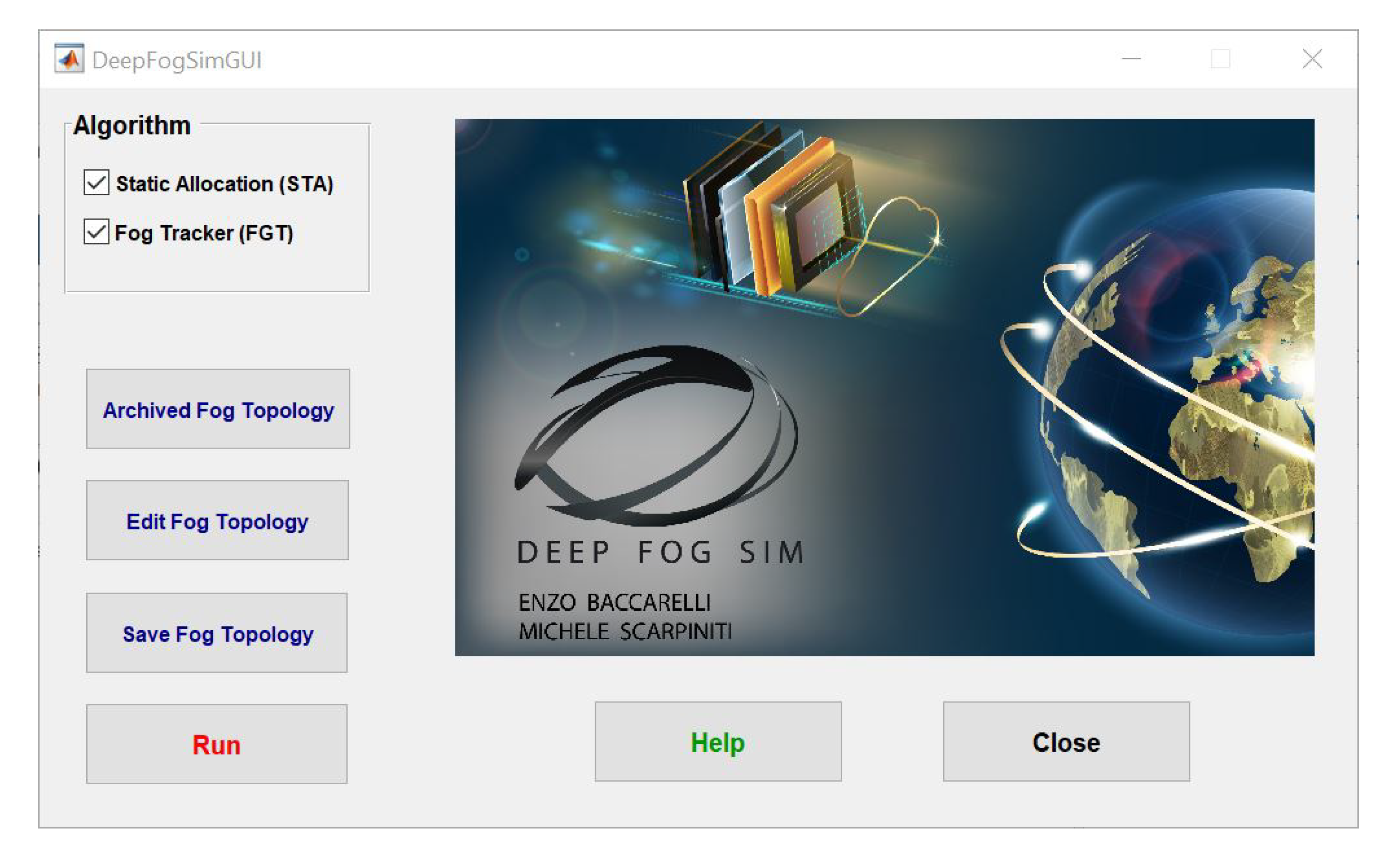
The current version of the DeepFogSim simulator is equipped with a (rich) Graphical User Interface (GUI) that displays:

• the numerical values of the best optimized frequencies for the convolutional and classifier processors and the network throughputs; and
• the numerical values of the optimal energy consumption, which are returned by the DynDeF_RAS function.

5.2. Supported Resource Allocation Strategies

In this subsection, we describe the supported resource allocation strategies provided by the DeepFogSim toolkit and listed in Table 2.

(a) The RAS function

The DynDeF_RAS function implements the primal-dual adaptive iterations in (25) and (27) for the numerical evaluation of the solution of the optimization problem in (23). The goal is to perform the optimized constrained allocation of the computing and networking resources needed by the simulated hierarchical Fog platform of Figure 3 for sustaining the inference phase of the CDNN of Figure 1a running atop it. The input parameters of this function are the following four vectors: $\left\{\overrightarrow{f_0},{\overrightarrow{\tilde{f}}}_0,{\overrightarrow{R}}_0,{\overrightarrow{\lambda }}_0\right\}$, which are needed for the initialization of the primal-dual iterations in (24) and (25). The values of these vectors are set by calling the main script of the DeepFogSim simulator.

The DynDeF_RAS function returns, by saving the values to the corresponding global variables, the following output variables:

• $\left[f_{mtx}\right]\in {\mathbb{R}}^{Q\times I_{MAX}}$ (bit/s): the matrix collecting the frequencies of the convolutional processors on a per-iteration basis;
• $\left[{\tilde{f}}_{mtx}\right]\in {\mathbb{R}}^{Q\times I_{MAX}}$ (bit/s): the matrix collecting the frequencies of the classifier processors on a per-iteration basis;
• $\left[R_{mtx}\right]\in {\mathbb{R}}^{(M-1)\times I_{MAX}}$ (bit/s): the matrix collecting the frequencies of the network throughputs on a per-iteration basis;
• $\left[{\lambda }_{mtx}\right]\in {\mathbb{R}}^{M\times I_{MAX}}$ (Joule): the matrix collecting the lambda multipliers on a per-iteration basis;
• $\overrightarrow{{\mathcal{E}}_{TOT}}\in {\mathbb{R}}^{1\times I_{MAX}}$ (Joule): the vector collecting the total energy in (20) on a per-iteration basis;
• $\overrightarrow{{\mathcal{E}}_{COP}}\in {\mathbb{R}}^{1\times I_{MAX}}$ (Joule): the vector collecting the computing energy in (21) on a per-iteration basis; and
• $\overrightarrow{{\mathcal{E}}_{NET}}\in {\mathbb{R}}^{1\times I_{MAX}}$ (Joule): the vector collecting the network energy in (22) on a per-iteration basis,

where the $I_{MAX}$ parameter fixes the maximum number of the allowed primal-dual iterations.

The last column of the previous matrices and vectors are the optimized (best) values of the allocated resources and consumed energy, respectively: ${\overrightarrow{f}}^{\left(best\right)}$, ${\overrightarrow{\tilde{f}}}^{\left(best\right)}$, ${\overrightarrow{R}}^{\left(best\right)}$, ${\overrightarrow{R}}^{\left(best\right)}$, ${\mathcal{E}}_{TOT}^{\left(best\right)}$, ${\mathcal{E}}_{COP}^{\left(best\right)}$, and ${\mathcal{E}}_{NET}^{\left(best\right)}$, which represent the final output of the DynDeF_RAS function.

Algorithm 1 presents a pseudo-code of the DynDeF_RAS function. An examination of this code points out that the asymptotic computational complexity of the DynDeF_RAS function scales linearly with $I_{MAX}$.

Algorithm 1DynDeF_RAS function

function: $DynDeF\_RAS\left(\overrightarrow{f_0},{\overrightarrow{\tilde{f}}}_0,{\overrightarrow{R}}_0,{\stackrel{\lambda }{R}}_0\right)$. Input: The initialized values: ${\overrightarrow{f}}_0,{\overrightarrow{\tilde{f}}}_0,{\overrightarrow{R}}_0,{\overrightarrow{R}}_0$. Output: ${\overrightarrow{f}}^{\left(best\right)}$, ${\overrightarrow{\tilde{f}}}^{\left(best\right)}$, and ${\overrightarrow{R}}^{\left(best\right)}$ vectors of the best resource allocation; scalar total energy ${\mathcal{E}}_{TOT}^{\left(MAX\right)}$ (Joule), scalar computing energy ${\mathcal{E}}_{COP}^{\left(MAX\right)}$ (Joule), and network energy ${\mathcal{E}}_{NET}^{\left(MAX\right)}$ (Joule) consumed under the optimized allocation vectors.

▹ Begin DynDeF_RAS function

1: for$m=1:M$do 2:     for $j=1:m_m$ do 3:          Compute $v_I(j,m)$ with Equation (1) 4:          Compute $v_O(j,m)$ with Equation (2) 5:     end for 6: end for 7: for$t=1:I_{MAX}$do                                               ▹RAS iterations 8:     for $m=1:M$ do 9:         for $j=1:m_m$ do 10:             Compute the $T_{EXE}(j,m)$ with Equations (3) and (4) 11:         end for 12:          Compute $T_{EXE}\left(m\right)$ with Equation (5) 13:     end for 14:      Compute $T_{EXE}^{(1,m)}$ with Equation (6) 15:      Compute ${\mathcal{E}}_{COP}$ with Equations (9), (11), and (21) 16:      Compute ${\mathcal{E}}_{NET}$ with Equation (22) 17:      Compute ${\mathcal{E}}_{TOT}$ with Equation (20) 18:      Compute all the derivatives of the Lagrangian function 19:      Update $\overrightarrow{f}$, $\overrightarrow{\tilde{f}}$, and $\overrightarrow{R}$ with Equations (24) and (25) 20:      Update $\overrightarrow{\lambda }$, $\overrightarrow{\alpha }$, and $\overrightarrow{\xi }$ with Equations (26) and (27) 21: end for 22: Obtain ${\overrightarrow{f}}^{\left(best\right)}$, ${\overrightarrow{\tilde{f}}}^{\left(best\right)}$, and ${\overrightarrow{R}}^{\left(best\right)}$ 23: Compute ${\mathcal{E}}_{COP}^{\left(best\right)}$ with Equations (9), (11), and (21) 24: Compute ${\mathcal{E}}_{NET}^{\left(MAX\right)}$ with Equation (22) 25: Compute ${\mathcal{E}}_{TOT}^{\left(MAX\right)}$ with Equation (20) 26: return$\left[{\overrightarrow{f}}^{\left(best\right)},{\overrightarrow{\tilde{f}}}^{\left(best\right)},{\overrightarrow{R}}^{\left(best\right)},{\mathcal{E}}_{TOT}^{\left(best\right)},{\mathcal{E}}_{COP}^{\left(best\right)},{\mathcal{E}}_{NET}^{\left(best\right)}\right]$.                ▹End DynDeF_RAS function

(b) The Static Allocation strategy

The Static Allocation strategy, implemented by the Static_Allocation function, calculates the computing, networking, and total energy consumed by the simulated Fog platform of Figure 3 for sustaining the delay-constrained inference phase of the considered CDNN under the (static) maximal allocation vectors: $\left\{{\overrightarrow{f}}^{\left(MAX\right)},{\overrightarrow{\tilde{f}}}^{\left(MAX\right)},{\overrightarrow{R}}^{\left(MAX\right)}\right\}$.

Hence, the Static_Allocation function returns:

• ${\mathcal{E}}_{TOT}^{\left(MAX\right)}$: the maximum total energy consumed by the the simulated Fog platform of Figure 3 under the maximal resource vectors;
• ${\mathcal{E}}_{COP}^{\left(MAX\right)}$: the maximum computing energy consumed by the the simulated Fog platform of Figure 3 under the maximal resource vectors; and
• ${\mathcal{E}}_{NET}^{\left(MAX\right)}$: the maximum network energy consumed by the the simulated Fog platform of Figure 3 under the maximal resource vectors.

Algorithm 2 presents a pseudo-code of the implemented Static_Allocation function. An examination of this code points out that the asymptotic computational complexity of the Static_Allocation function scales linearly with the sum of M of tiers and the total number Q of Fog nodes, i.e., $M+Q$.

Algorithm 2Static_Allocation function

function: $Static\_Allocation$. Input: $FanIn(j,m)$, $FanOut(j,m)$, ${\overrightarrow{f}}^{\left(MAX\right)}$, ${\overrightarrow{\tilde{f}}}^{\left(MAX\right)}$, and ${\overrightarrow{R}}^{\left(MAX\right)}$. Output: scalar total energy ${\mathcal{E}}_{TOT}^{\left(MAX\right)}$ (Joule), scalar computing energy ${\mathcal{E}}_{COP}^{\left(MAX\right)}$ (Joule), and network energy ${\mathcal{E}}_{NET}^{\left(MAX\right)}$ (Joule) consumed under the maximal allocation vectors.

▹Begin Static_Allocation function

1: for$m=1:M$do 2:     for $j=1:m_m$ do 3:          Compute $v_I(j,m)$ with Equation (1) 4:          Compute $v_O(j,m)$ with Equation (2) 5:          Compute the $T_{EXE}(j,m)$ with Equations (3) and (4) 6:     end for 7:      Compute $T_{EXE}\left(m\right)$ with Equation (5) 8: end for 9: Compute $T_{EXE}^{(1,m)}$ with Equation (6) 10: Compute ${\mathcal{E}}_{COP}^{\left(MAX\right)}$ with Equations (9), (11), and (21) 11: Compute ${\mathcal{E}}_{NET}^{\left(MAX\right)}$ with Equation (22) 12: Compute ${\mathcal{E}}_{TOT}^{\left(MAX\right)}$ with Equation (20) 13: return$\left[{\mathcal{E}}_{TOT}^{\left(MAX\right)},{\mathcal{E}}_{COP}^{\left(MAX\right)},{\mathcal{E}}_{NET}^{\left(MAX\right)}\right]$.       ▹End Static_Allocation function

5.3. Auxiliary Functions of DeepFogSim

In this subsection, we provide the description of some auxiliary functions called from the previous main routines. These auxiliary functions are listed in Table 3.

The Check_convexity function checks for the (strict) convexity of the optimization problem in (23). If the problem is not strictly convex, the function returns an error message and then exits the program.

The Check_feasibility function tests the (strict) feasibility of the underlying constrained optimization problem in (23) by checking M delay-induced constraints in (23b). If at least one of these M constraints fails, the function generates an error message indicating the failed delay constraint and then stops the overall program.

In a similar way, the Check_input function checks for the formal validity of the input data set by the user. If any input variable is not formally valid, the function returns an error message and then exits the program.

The init_other_global function initializes all the output and dummy (global) variables that have not been directly set by the user in the configuration script.

Finally, the oneDtotwoD and twoDtooneD functions allow transformation of the mono-dimensional (i.e., string type) representation of the network topology of Figure 3 to the corresponding bi-dimensional one. Specifically, these functions are used to map the bi-dimensional index of the i-th Fog node lying in the j-th tier into a sequential scalar number falling in the range $1,\dots ,Q$. In more detail:

• The function [tier, column] = oneDtotwoD(oneDindex) converts the 1D indexing of a Fog node to the corresponding 2D row/column one. The input parameter $oneDindex$ must be an integer and fall in the range: $1,\dots ,Q$. The returned $tier$ parameter is an integer and falls in the range: $1,\dots ,M$. The returned corresponding $column$ parameter is an integer and falls in the range: $1,\dots ,m_m$.
• The function oneDindex = twoDtooneD(tier, column) evaluates the 1D equivalent index of the 2D indexing of a Fog node. The returned $oneDindex$ is integer-valued and falls in the range: $1,\dots ,Q$. The value of the tier parameter must be an integer and fall in the range: $1,\dots ,M$. The value of the column parameter must be an integer and fall in the interval: $1,\dots ,m_m$.

5.4. DynDeFog_TRACKER: The Dynamic Performance Tracking Function

The goal of the DynDeFog_TRACKER function is to test the convergence rate to the steady state and the steady-state stability of the primal-dual iterations performed by the DynDeF_RAS function when unpredicted and abrupt changes in the operating conditions of the simulated Fog platform of Figure 3 happen. These changes are formally dictated by the scaling vectors: ${\overrightarrow{jump}}_1$ and ${\overrightarrow{jump}}_2$ (see Table A2), which multiply the scalar components of the input maximal resource allocation vector: $\left[{\overrightarrow{v}}_0,{\overrightarrow{f}}^{\left(MAX\right)},{\overrightarrow{\tilde{f}}}^{\left(MAX\right)},{\overrightarrow{R}}^{\left(MAX\right)}\right]$. Specifically, at the time indexes multiple of $\left((k/5)\times iter\_number\right)+1$, with $k=1,\dots ,5$, the initial values of the sliced resource vector: $\left[{\overrightarrow{v}}_0,{\overrightarrow{f}}^{\left(MAX\right)},{\overrightarrow{\tilde{f}}}^{\left(MAX\right)},{\overrightarrow{R}}^{\left(MAX\right)}\right]$, undergo changes. These changes are obtained by multiplying (on a per scalar entry-basis) the components of the sliced vector $\left[{\overrightarrow{v}}_0,{\overrightarrow{f}}^{\left(MAX\right)},{\overrightarrow{\tilde{f}}}^{\left(MAX\right)},{\overrightarrow{R}}^{\left(MAX\right)}\right]$ by: ${\overrightarrow{jump}}_1$ and ${\overrightarrow{jump}}_2$.

The input parameters of the DynDeFog_TRACKER function are the same ones of the DynDeF_RAS function, namely $\overrightarrow{f_0}$, ${\overrightarrow{\tilde{f}}}_0$, ${\overrightarrow{R}}_0$, and ${\overrightarrow{\lambda }}_0$. The outputs of the DynDeFog_TRACKER function are the resulting time-traces of the computing energy, network energy, total energy, ${\lambda }_1$ multiplier and ${\lambda }_M$ multiplier over the time interval $(1,iter\_number)$, evaluated for three values of the speed-up factor $a_{MAX}$ (stored into the $(1\times 3)$ input vector ${\overrightarrow{a}}_{MAX}$).

The feasibility of the operating conditions induced by ${\overrightarrow{jump}}_1$ and ${\overrightarrow{jump}}_2$ are explicitly tested by the DynDeFog_TRACKER function, and suitable terminating error messages are generated if infeasible operating conditions occur.

Graphic plots of the time traces of the returned output matrices are displayed at the end of the DynDeFog_TRACKER run. A detailed description of each of the steps performed by the DynDeFog_TRACKER can be found in the User Guide of the DeepFogSim package. From the previous description, it follows that the asymptotic complexity of the DynDeFog_TRACKER function scales up as in: $\mathcal{O}\left(\left(2(Q+M)-1\right)\times iteration\_number\times 3\right)$.

Overall,

Table 4. A synoptic overview of the computational complexities of the main functions supported by the DeepFogSim toolkit.

Function	Asymptotic Computational Complexity
DynDeF_RAS	$\mathcal{O}\left(I_{MAX}\left(2(Q+M)-1\right)\right)$
Static_Allocation	$\mathcal{O}\left(2(Q+M)-1\right)$
DynDeFog_TRACKER	$\mathcal{O}\left(\left(2(Q+M)-1\right)\times iter\_number\times 3\right)$

presents a synoptic view of the asymptotic computational complexities of the described DynDeF_RAS, Static_Allocation, and DynDeFog_TRACKER functions.

6. DeepFogSim: Supported Formats of the Rendered Data

Under the current version of the simulator, both the DeepFogSim and DeepFogSimGUI interfaces (see Appendix A) support four main formats, in order to render the results output by the three main routines of Table 4. The functions, used to obtain these formats, are listed in

Table 5. Rendering functions for the supported formats implemented in DeepFogSim.

Function	Description
plot_Topology()	Implements the Fog topology format.
$\mathrm{print\_solution}\left(strategy\right)$	Implements the tabular format.
$fignumber=\mathrm{plot\_solution}\left(fignumber,options\right)$	Implements the colored graphic plot format.
$fignumber=\mathrm{plot\_FogTracker}\left(fignumber\right)$	Implements the colored time-tracker plot format.

and are described in depth in the DeepFogSim User Guide (see Section 9). These rendering formats are:

• the Tabular format, which is enabled by the print_solution graphic function;
• the Colored Graphic Plot format, which is enabled by the plot_solution graphic function;
• the Colored Time-tracker Plot format, which is enabled by the plot_FogTracker graphic function; and
• the Fog Topology format, which is enabled by the plot_Topology graphic function.

Specifically, the print_solution function prints on the MATLAB prompt the result obtained by running the tested strategies under the selected topology and given input parameters (see Table A2). This function has an optional input parameter that allows the print of the results obtained by the DynDeF_RAS function and the Static_Allocation function, respectively. The function prints, in a numerical form, the results related to the optimized frequencies of the convolutional and classifier processors, the optimized energies ${\mathcal{E}}_{TOT}^{\left(best\right)}$, ${\mathcal{E}}_{COP}^{\left(best\right)}$, and ${\mathcal{E}}_{NET}^{\left(best\right)}$, and the ratio ${\mathcal{E}}_{NET}^{\left(best\right)}/{\mathcal{E}}_{TOT}^{\left(best\right)}$. If the Static_Allocation is selected in the main script, it also prints the maximum energies ${\mathcal{E}}_{TOT}^{\left(MAX\right)}$, ${\mathcal{E}}_{COP}^{\left(MAX\right)}$, and ${\mathcal{E}}_{NET}^{\left(MAX\right)}$ consumed by the maximal resource allocation strategy and the ratio ${\mathcal{E}}_{NET}^{\left(MAX\right)}/{\mathcal{E}}_{TOT}^{\left(MAX\right)}$. In addition, the print_solution function prints on the MATLAB prompt the total computing time needed for running all the selected strategies.

The plot_solution function opens a number of figure windows, which graphically display the numerical results obtained by the DeepFogSim simulator. This function accepts two optional input parameters, i.e., (i) the number of figure from which to start and (ii) a flag used to choose whether the results returned by the Static_Allocation function must be also plotted. A maximum of eleven different figures may be opened. Specifically, this function displays the traces of the resources allocated by the DynDeF_RAS function (and eventually by the Static_Allocation one) and the related consumed total, computing and networking energy. A figure showing a bar plot of the per-exit actual-vs.-maximum tolerated delay ratio is also provided.

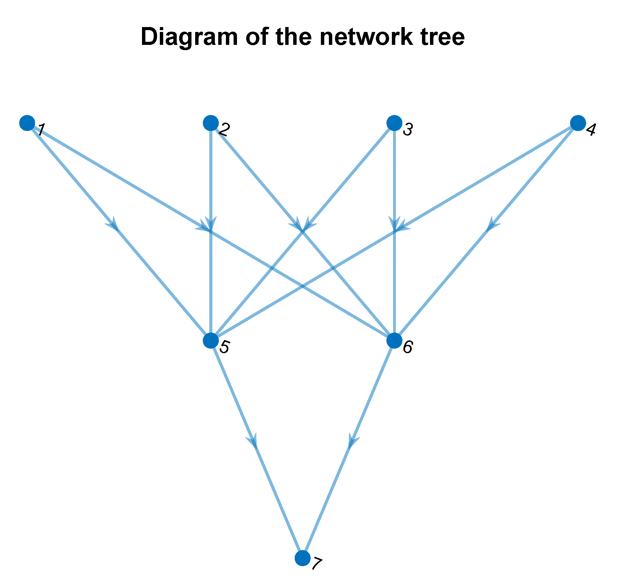
The plot_Topology function returns a graphic representation of the Fog topology set in the input configuration for the Fog platform to be simulated. This function reads the global matrix variable $\left(A\right)$, which represents the adjacency matrix of the tree. An illustrative screenshot of the network tree plot by this function is shown in Figure 7.

Finally, the plot_FogTracker function provides the graphic capabilities needed for a proper plot of the time-traces of the total energy, computing energy and networking energy, and the first and last lambda multipliers generated by the DynDeFog_TRACKER function under the three values of step-size that are stored by the input vector ${\overrightarrow{a}}_{FogT}^{\left(MAX\right)}$ (see

Table A1. A synoptic overview of the functionalities offered to the user by the DeepFogSimGUI interface.

Available GUI Functions	Associated Actions
Help	Allows to access the User Guide of the simulator by opening a dedicated PDF file.
Algorithm	Allows to select any subset of the natively supported optimization algorithms by clicking the corresponding labels.
Archived Fog Topology	Allows to retrieve an already archived Fog topology with the corresponding simulation setup, in order to run it.
Edit Fog Topology	Allows to edit a new Fog topology and/or a new simulation setup by compiling the list of input parameters of Table A1.
Save Fog Topology	Allows to save the lastly edited Fog topology and assigns it an identification label.
Run	Allows to run the selected optimization algorithm under the retrieved/edit Fog topology and associated simulation setup.
Close	Shuts down the current working session of the DeepFogSim simulator and closes all the figure windows.

). Its input parameter is the number of figure from which to start, to be sequential from the last plotted figure. Specifically, the function renders five figures that orderly report: the total (computing-plus-networking), computing, and networking energy, and the first and last lambda multiplier. All curves have been evaluated under the three step-size values stored by the input ${\overrightarrow{a}}_{FogT}^{\left(MAX\right)}$ vector. Some illustrative screenshots of the dynamic plots rendered by the FogTracker function are shown in Figures 15 and 16 of Section 7.3.

In the current version of the DeepFogSim package, it is available an archive that stores several test setups, together with the related sets of (suitably tuned) input parameters. These Fog topologies are ready-for-the-use, i.e., they may be retrieved by the user and then run under both the (previously described) interfaces of the simulator. The archived set-ups cover several topologies, with different number of tiers and per-tier nodes. Specifically, the number of Fog nodes ranges from $Q=7$, to $Q=63$, the number of tiers ranges from $M=3$ to $M=6$, while the number of links varies in the range $(10,682)$.

7. Performance Evaluation

This section aims at showing the actual capabilities of the developed DeepFogSim toolkit by numerically testing and comparing the energy-delay-tracking performance of its natively supported optimization tools of Section 5 under some use cases of practical interest.

The peculiar features of the considered CDNN with early exits is the presence of a number of hierarchically organized delay-constraints (see Equation (23b)) on the allowed per-exit maximum tolerated inference times. To the best of authors’ knowledge, neither resource allocation algorithms nor related simulation packages are currently present in the open literature, which explicitly consider these multiple inference delays featuring the considered operating framework. Hence, motivated by this consideration, the proposed DeepFogSim simulator natively supports, as a benchmark for performance comparison, the so-called Maximal Resource Allocation strategy of Algorithm 2. This is a not adaptive resource allocation strategy that takes fixed at their allowed maximum values all the components of the resource allocation vectors $\left\{{\overrightarrow{f}}^{\left(MAX\right)},{\overrightarrow{\tilde{f}}}^{\left(MAX\right)},{\overrightarrow{R}}^{\left(MAX\right)}\right\}$. The performance comparisons against this benchmark allow us to appreciate, indeed, the actual resources savings arising from the implementation of the adaptive resource allocation engine of Algorithm 1 which is the core of the proposed DeepFogSim simulator.

A joint examination of the volumes of the input and output workloads in Equations (1) and (2) processed by the $(j,m)$-th FN, and the related model for the dynamic power profile ${\mathcal{P}}_{CON}^{\left(DYN\right)}(j,m)$ of the $(j,m)$-th convolutional processor in Equation (8), points out that the information about the CDNN with early exits, needed for running the DeepFogSim simulator are [15]: (i) the vector of the per-layer compression factors $\overrightarrow{cm}\triangleq {\left[c{m}_1,\dots ,c{m}_{L-1}\right]}^T\in {\mathbb{R}}_{+}^{L-1}$, where $c{m}_l$, $1\le l\le L-1$, is the ratio between the size (in bit) of the workload at the output from $layer\#l$ with respect to that at its input (i.e., $0\le c{m}_l\le 1$ takes account of the fraction of the workload that does not undergo early exit); and (ii) the vector of the Layer-to-Tier mappings featured by the actually performed partition ${\overrightarrow{L2T}}_{map}\triangleq {\left[\left|{\mathcal{T}}_1\right|,\dots ,\left|{\mathcal{T}}_M\right|\right]}^T\in {\mathbb{N}}_{+}^M$, where $\left|{\mathcal{T}}_m\right|$, $1\le m\le M$, is the number of (adjacent) CDNN layers in Figure 1a mapped onto the m-the tier in Figure 1b.

An in-depth analysis and evaluation of the overall topic of the optimized design of CDNNs with early exits is presented in Reference [15], together with numerical examples of the vectors $\overrightarrow{cm}$ and ${\overrightarrow{L2T}}_{map}$ for some CDNNs of practical interest (see, in particular, Tables 4–6 of Reference [15] and the related texts). As already detailed in Reference [15], we note that, in practice, the actual values of these vectors depend on a number of design factors, like the topology of the considered CDNN, the number and placement of the corresponding early exits, the sets of examples used to train and validate the CDNN, just to name a few.

All the simulations have been carried out by exploiting an hardware execution platform equipped with: (i) an Intel 10-core i9-7900X processor; (ii) 32 GB of RAM DDR 4; (iii) an SSD with 512 GB plus an HDD with 2TB; and (iv) a GPU ZOTAC GeForce GTX 1070. The release R2020a of MATLAB provided the underlying software execution platform.

We remark that, unless otherwise stated, all the simulations have been carried out under the parameter setting reported in the last column of the final Table A2 in Appendix B.

7.1. Use Cases and Simulated Fog Topologies

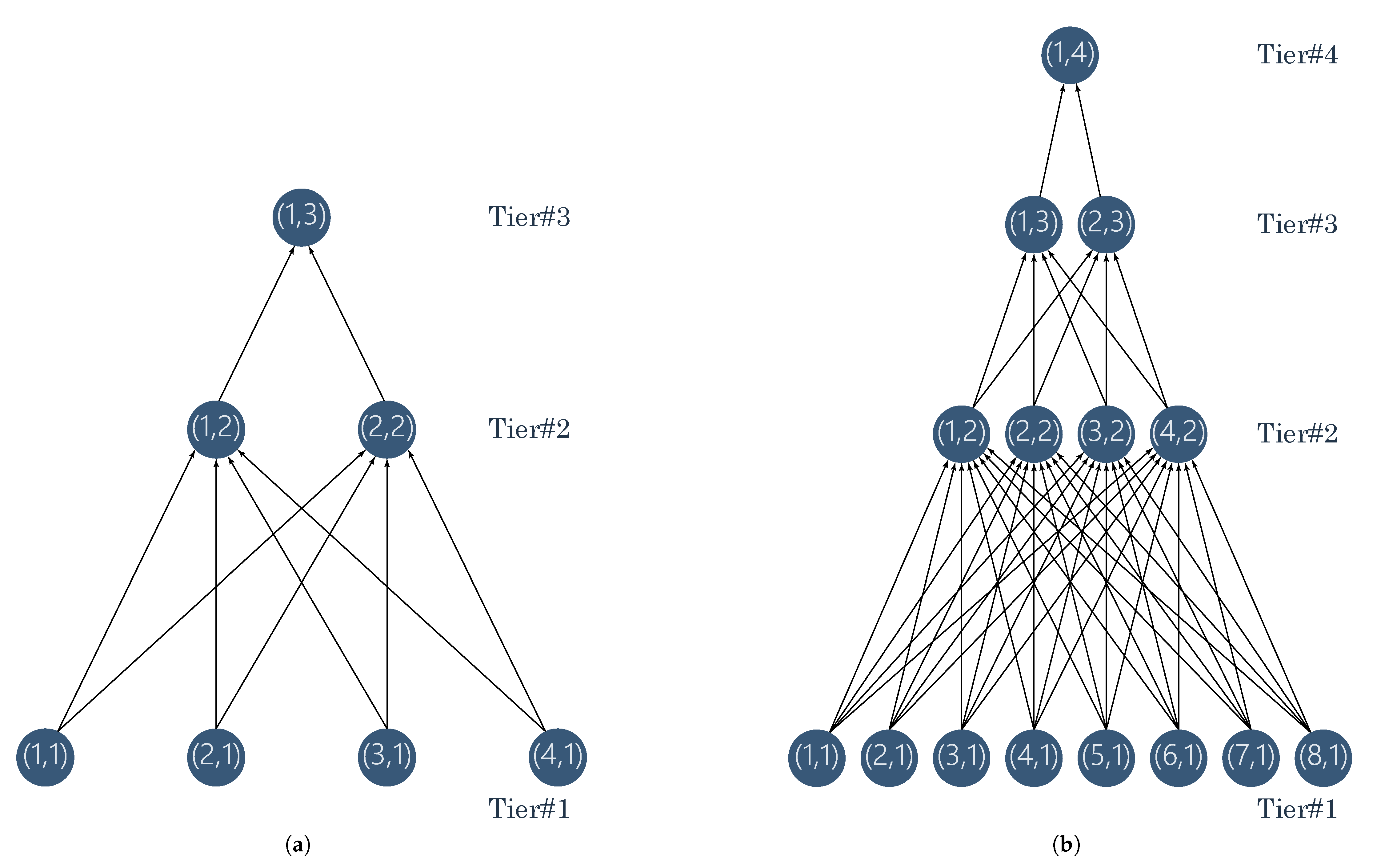
The reported tests of the DeepFogSim package refer to the Fog topologies sketched in Figure 8, hereinafter referred to as $T1$ and $T2$, respectively. Specifically:

• topology $T1$ is composed of $Q=9$ nodes, which are arranged onto $M=3$ tiers. Each node at $tier\#m$ is connected to every node at $tier\#(m+1)$; hence, the $T1$ topology embraces 10 transmission links;
• topology $T2$ is composed of $Q=15$ nodes, which are arranged onto $M=4$ tiers. Each node at $tier\#m$ is connected to every node at $tier\#(m+1)$; hence, the resulting $T2$ topology embraces 42 transmission links.

Due to space constraints, we have decided to limit to report the performance results under $T1$ and $T2$ topologies. However, the archived set-ups in the DeepFogSim package cover several topologies, with different number of tiers and per-tier nodes.

In the carried out simulations, we refer to a CDNN with $L=9$ layers to be suitably scattered over the available M tiers of the Fog platform of Figure 1b. In particular, we assume the following default numerical settings:

• ${\overrightarrow{cm}}^{\left(0\right)}={\left[0.045,0.1,0.3,0.5,0.71,0.7,0.7,0.9,0.9\right]}^T$ for the compression vector;
• ${\overrightarrow{L2T}}_{map}^{\left(0\right)}={\left[4,2,1\right]}^T$ and ${\overrightarrow{cm}}_{map}^{\left(0\right)}={\left[2,2,2,2\right]}^T$ for the mapping vectors under the two considered Fog topologies $T1$ and $T2$, respectively; and
• ${\overrightarrow{T}}_{EXIT}^{\left(0\right)}={\left[T_S,T_S,0.4T_S\right]}^T$ (s) and ${\overrightarrow{T}}_{EXIT}^{\left(0\right)}={\left[T_S,T_S,T_S,0.4T_S\right]}^T$ (s) for the per-tier maximum allowed inference times under the two considered topologies in Figure 8.

In addition, in the carried out simulations, we set the maximum allowable resources to: $f_{jm}^{\left(MAX\right)}=9$ (Mbit/s), ${\tilde{f}}_{jm}^{\left(MAX\right)}=8$ (Mbit/s), $R_1^{\left(MAX\right)}=8$ (Mbit/s), and $R_2^{\left(MAX\right)}=9$ (Mbit/s) under topology $T1$ and to: $f_{jm}^{\left(MAX\right)}=4.2$ (Mbit/s), ${\tilde{f}}_{jm}^{\left(MAX\right)}=3.73$ (Mbit/s), and $R_m^{\left(MAX\right)}=1.95$ (Mbit/s) under topology $T2$. These values are the same for every node, i.e., for all $j=1,\dots ,M$ and $m=1,\dots ,m_m$.

7.2. Resource and Energy Distribution Returned by DeepFogSim

In this subsection, we provide results obtained by the DynDeF_RAS function in terms of both resource allocation and energy performance.

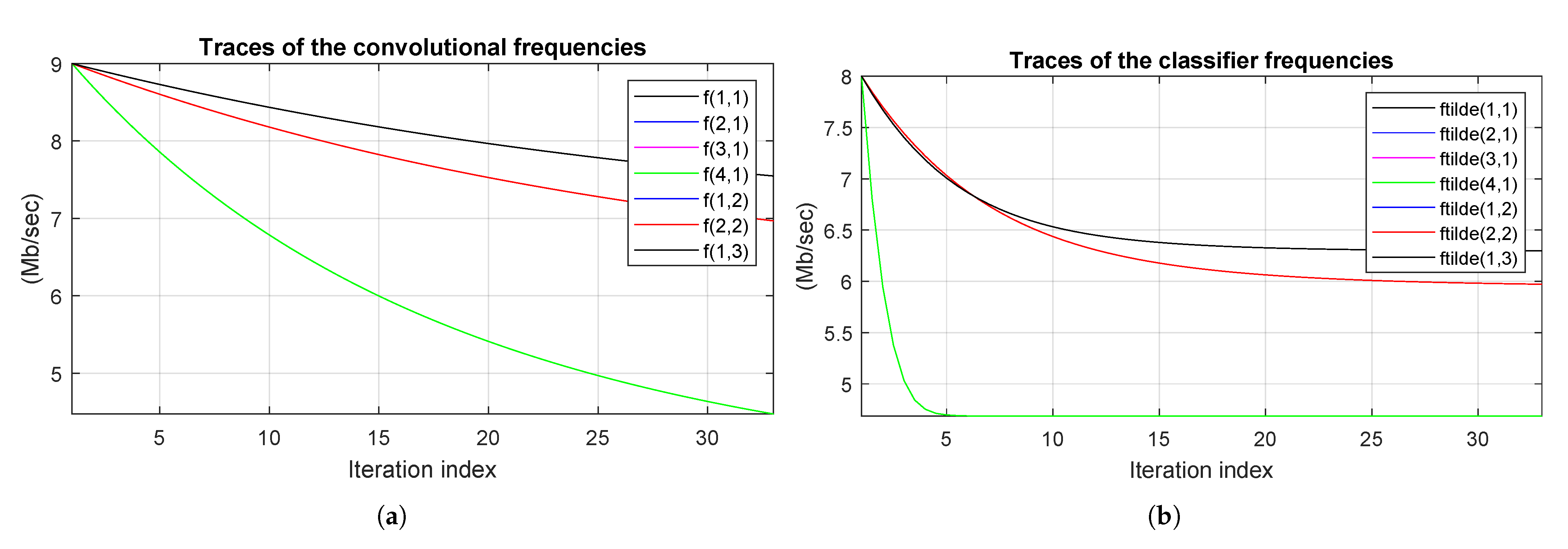
To begin with, the DeepFogSim has been tested under topology $T1$ and the obtained plots are shown in Figure 9. Specifically, Figure 9a,b illustrate the traces of the optimized frequencies of the convolutional and the classifier processors, respectively. Although the total number of iteration $I_{MAX}$ of the DynDeF_RAS function in Algorithm 1 is set to 450, these figures clearly show that the DeepFogSim simulator stops Algorithm 1 after only 33 iteration. An examination of the traces and legends shown in Figure 9a,b also suggests that all the involved frequencies (both for the convolutional and classifier processors) are clustered into three groups, which correspond to the FNs allocated over each of the three tiers of the considered Fog topology. This behavior is justified by the fact that, at each tier, each FN has to process the same volume of the input workload.

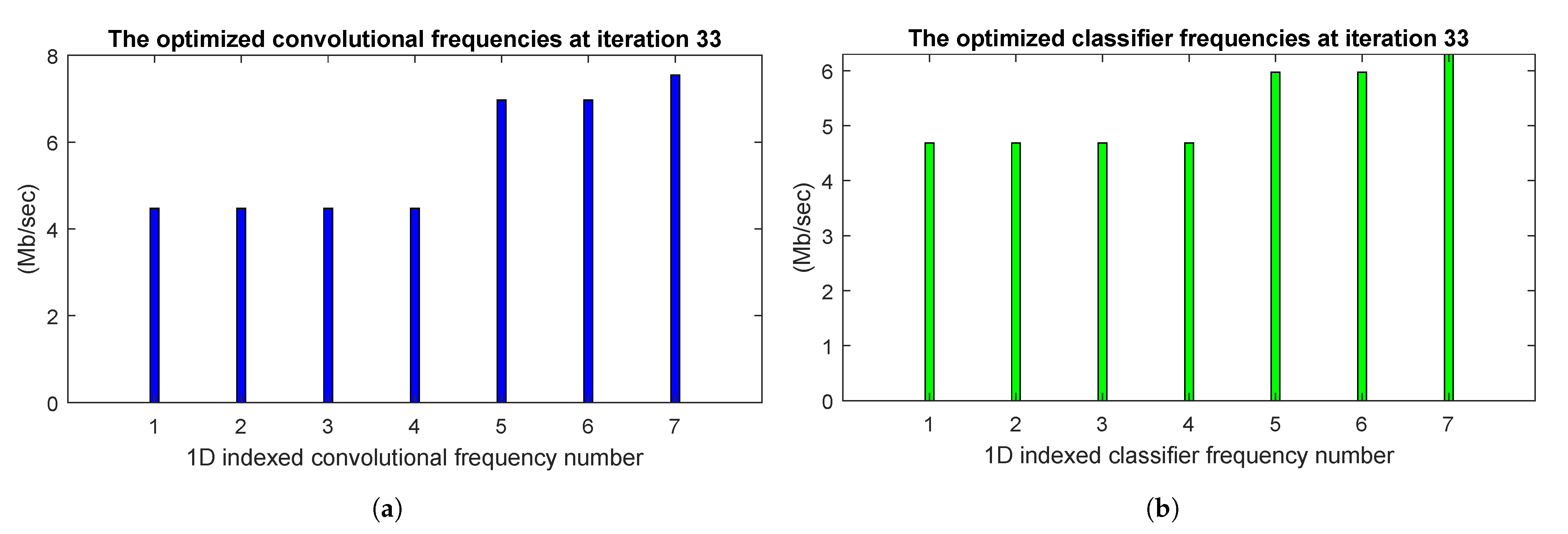
The last values of the traces in Figure 9a,b, i.e., the optimized frequencies of the convolutional and the classifier processors returned by the Algorithm 1, are shown in the bar plots of Figure 10a,b, respectively. These plots confirm the clusterization of the optimized frequencies of both the convolutional and the classifier processors: the four frequencies of the first tier converge to the same value, and a similar behavior holds for the two frequencies of the second tier.

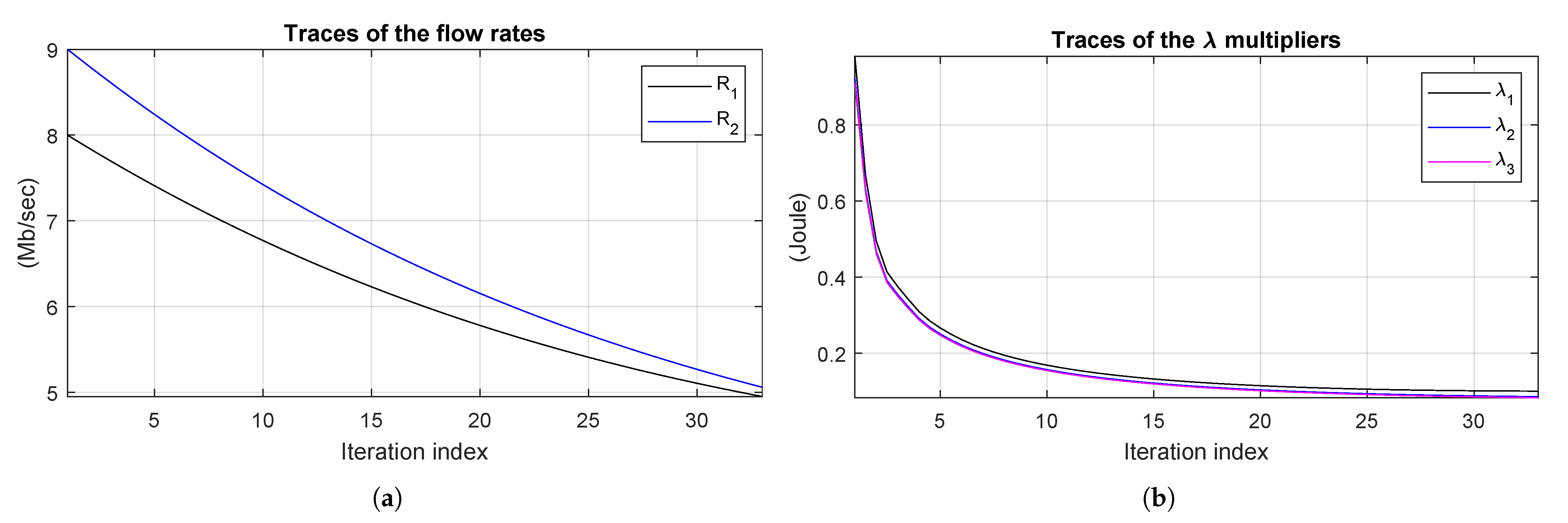
In a similar way, Figure 11a shows the traces of the optimized flow rates $R_1$ and $R_2$ between $tier\#1$ and $tier\#2$, and between $tier\#2$ and $tier\#3$, respectively. This figure shows that, although the rates start from different values, they converge to similar values at the steady state. Figure 11b illustrates the convergence of the lambda multipliers in (25) and supports the conclusion that a very limited number of iterations is sufficient to converge to a feasible solution.

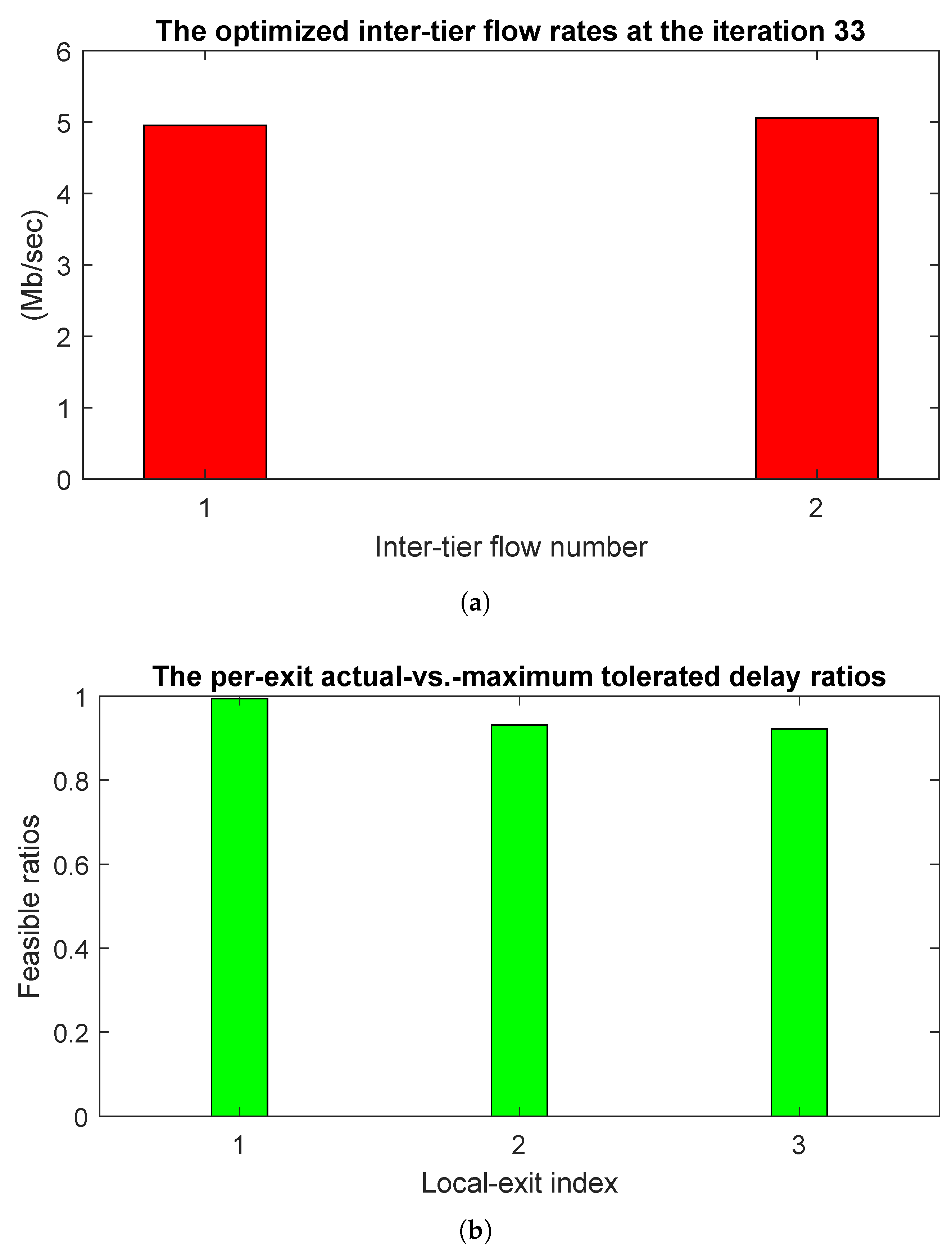
The values of the optimized values of the flow rates $R_1$ and $R_2$ are presented in Figure 12a, once again highlighting the similar optimized values. Figure 12b, instead, shows the ratio between the actual delay needed to perform the computation-plus-communi cation task at each tier in (6) and the maximum tolerated delays $T_{EXIT}$. By definition, the returned optimized solution is feasible if all these rates are not greater than the unit. Figure 12b clearly shows that this constraint is met in all the three cases; hence, the presented steady-state resource allocations are, indeed, feasible.

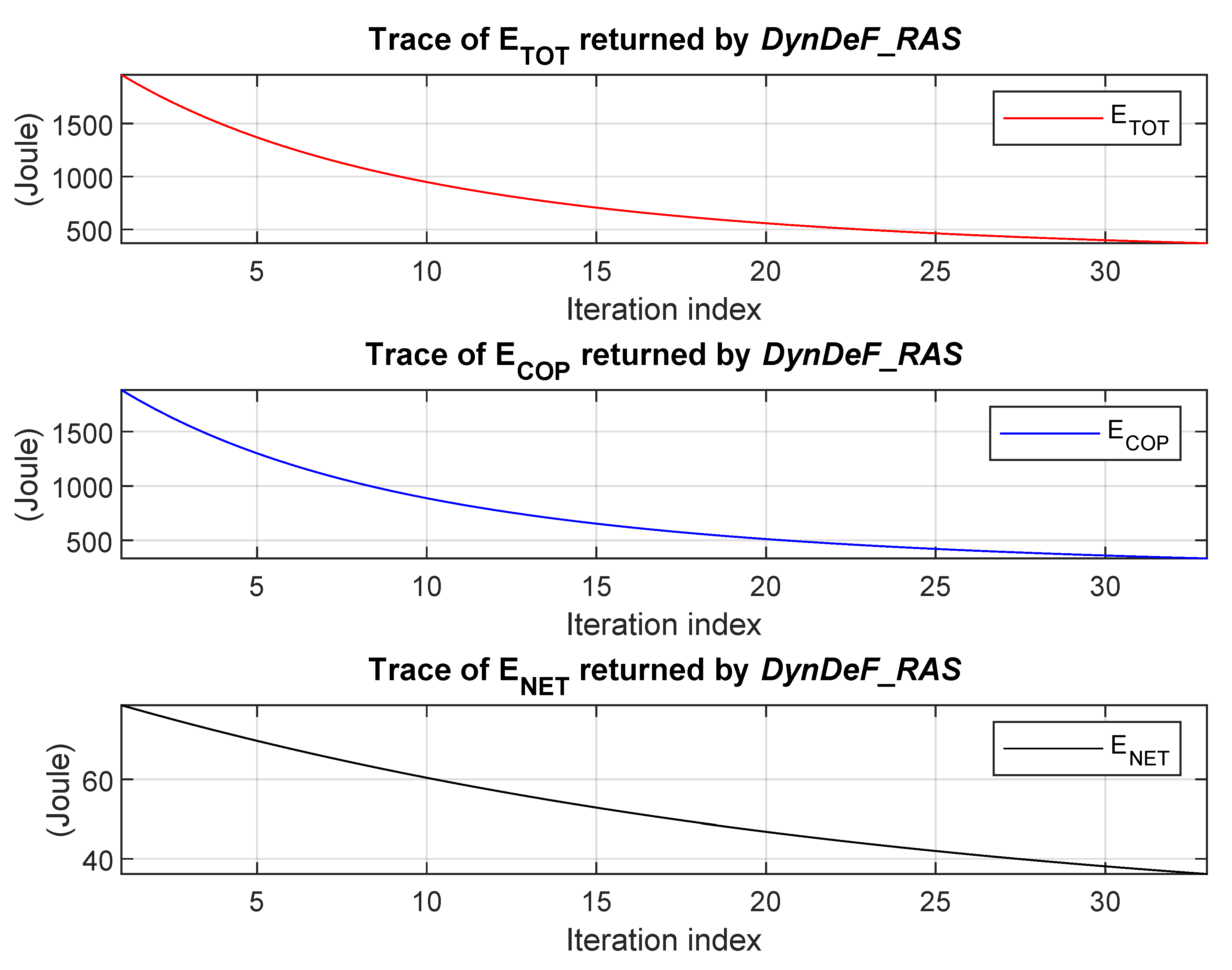
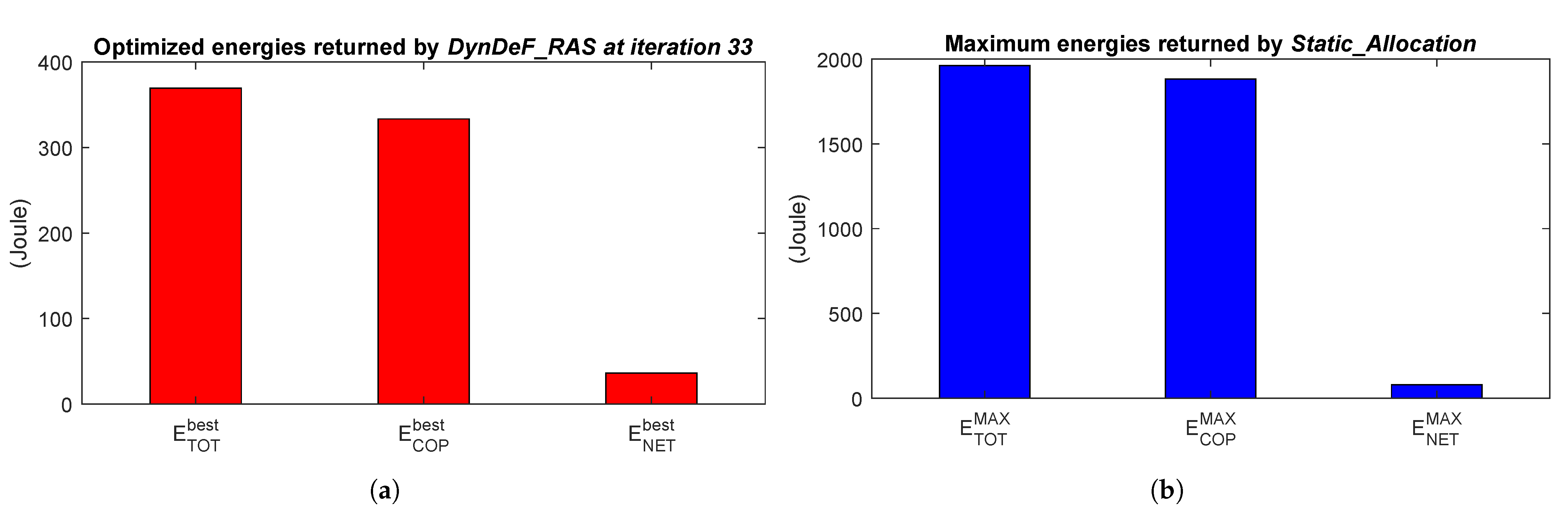
In order to describe the energy plots returned by the DeepFogSim toolkit, Figure 13 presents the returned traces of the total energy ${\mathcal{E}}_{TOT}^{\left(best\right)}$ (top plot), computing energy ${\mathcal{E}}_{COP}^{\left(best\right)}$ (middle plot), and network energy ${\mathcal{E}}_{NET}^{\left(best\right)}$ (bottom plot). In addition, for the energy consumption, it is evident that DeepFogSim allows a considerable saving after only 33 iteration of Algorithm 1. The final optimized values for these energies are shown by the bar plots of Figure 14a, which explicitly illustrate that the main fraction of the total consumed energy is due to the computing part, while the network one is limited up to about 10%.

In order to provide fair comparisons, Figure 14b presents the bar plots of the total energy ${\mathcal{E}}_{TOT}^{\left(MAX\right)}$, computation energy ${\mathcal{E}}_{COP}^{\left(MAX\right)}$, and network energy ${\mathcal{E}}_{NET}^{\left(MAX\right)}$ consumed in the case that all the available resources are set to their maximum values: $f_{ij}^{\left(MAX\right)}$, ${\tilde{f}}_{jm}^{\left(MAX\right)}$, and $R_m^{\left(MAX\right)}$. These energies are evaluated by the Static_Allocation function described in Section 5.2 and presented in Algorithm 2. A comparison of plots in Figure 14a,b demonstrates the noticeable energy saving offered by the adaptive Algorithm 1 implemented by the DeepFogSim toolkit.

A synoptic view of the energy consumption under topology $T1$, compared to the static allocation solution and the ratios between these two solutions, is analytically presented in the first row of

Table 6. Energy comparison under the test $T1$ and $T2$ Fog topologies.

Topology	${\mathcal{E}}_{\mathit{T}\mathit{O}\mathit{T}}^{\left(\mathit{M}\mathit{A}\mathit{X}\right)}$ (J)	${\mathcal{E}}_{\mathit{T}\mathit{O}\mathit{T}}^{\left(\mathit{b}\mathit{e}\mathit{s}\mathit{t}\right)}$ (J)	${\mathcal{E}}_{\mathit{C}\mathit{O}\mathit{P}}^{\left(\mathit{b}\mathit{e}\mathit{s}\mathit{t}\right)}$ (J)	${\mathcal{E}}_{\mathit{N}\mathit{E}\mathit{T}}^{\left(\mathit{b}\mathit{e}\mathit{s}\mathit{t}\right)}$ (J)	$\frac{{\mathcal{E}}_{\mathit{N}\mathit{E}\mathit{T}}^{\left(\mathit{b}\mathit{e}\mathit{s}\mathit{t}\right)}}{{\mathcal{E}}_{\mathit{T}\mathit{O}\mathit{T}}^{\left(\mathit{b}\mathit{e}\mathit{s}\mathit{t}\right)}}$ (%)	$\frac{{\mathcal{E}}_{\mathit{T}\mathit{O}\mathit{T}}^{\left(\mathit{M}\mathit{A}\mathit{X}\right)}}{{\mathcal{E}}_{\mathit{T}\mathit{O}\mathit{T}}^{\left(\mathit{M}\mathit{A}\mathit{X}\right)}}$ (%)
T1	1960.9	369.6	333.5	36.2	9.8 %	18.8 %
T2	1140.0	144.3	114.1	30.3	21.0 %	12.7 %
T1a	12148.7	1192.1	1017.2	174.9	14.7 %	9.8 %
T2a	12486.7	552.9	477.8	75.1	13.6 %	4.4 %

. This table also shows the ratio between the optimized network energy and the total one: ${\mathcal{E}}_{NET}^{\left(best\right)}/{\mathcal{E}}_{TOT}^{\left(best\right)}$.

Regarding the network topology $T2$, we have numerically ascertained that traces similar to those of the previous Figure 9, Figure 10, Figure 11, Figure 12, Figure 13 and Figure 14 are obtained; hence, we do not show them here. However under topology $T2$, Algorithm 1 converges within only 23 iterations. Once again, the number of needed iterations is very small.

The energy performance under the network topology $T2$ is also summarized in Table 6 (see the second row). Moreover, this table also presents the energy performance under topologies $T1$ and $T2$ by using a different Layer-to-Tier mapping vector ${\overrightarrow{L2T}}_{map}^{\left(0\right)}$ and different maximum allowable resources. We named this new tested settings as $T1a$ and $T2a$, respectively (see the 3rd and 4th rows in Table 6). The new sets of values are: ${\overrightarrow{L2T}}_{map}^{\left(0\right)}=[3,3,3]$, $f_{im}^{\left(MAX\right)}=9$ (Mbit/s), ${\tilde{f}}_{im}^{\left(MAX\right)}=8$ (Mbit/s), and $R_m^{\left(MAX\right)}=8.2$ (Mbit/s) under topology $T1a$; and ${\overrightarrow{L2T}}_{map}^{\left(0\right)}=[3,3,2,1]$, $f_{im}^{\left(MAX\right)}=9$ (Mbit/s), ${\tilde{f}}_{im}^{\left(MAX\right)}=8$ (Mbit/s), and $R_m^{\left(MAX\right)}=9$ (Mbit/s) under topology $T2a$.

An examination of the related rows of Table 6 shows that the adaptive Algorithm 1, in all tested cases, allows a considerable energy saving with respect to the benchmark static one of Algorithm 2. In addition, Table 6 suggests that Fog topologies with higher numbers of tiers generally allow greater savings with respect to topologies with fewer numbers of tiers. This is justified by the fact that better distributions of the workload may be attained over a greater number of nodes at the first tier and greater fractions of the workload undergo to early exit for increasing number of the topology tiers.

The energy sensitivity of the resource allocation returned by DeepFogSim is measured at different values of the vector ${\overrightarrow{T}}_{EXIT}$ (s) of the maximum allowed inference times under topology $T2$ and the results are comparatively presented in

Table 7. Energy sensitivity on the vector ${\overrightarrow{T}}_{EXIT}$ (s) of the maximum allowed inference times under the simulated topology $T2$.

${\overrightarrow{\mathit{T}}}_{\mathit{E}\mathit{X}\mathit{I}\mathit{T}}$ (s)	${\mathcal{E}}_{\mathit{T}\mathit{O}\mathit{T}}^{\left(\mathit{M}\mathit{A}\mathit{X}\right)}$ (J)	${\mathcal{E}}_{\mathit{T}\mathit{O}\mathit{T}}^{\left(\mathit{b}\mathit{e}\mathit{s}\mathit{t}\right)}$ (J)	${\mathcal{E}}_{\mathit{C}\mathit{O}\mathit{P}}^{\left(\mathit{b}\mathit{e}\mathit{s}\mathit{t}\right)}$ (J)	${\mathcal{E}}_{\mathit{N}\mathit{E}\mathit{T}}^{\left(\mathit{b}\mathit{e}\mathit{s}\mathit{t}\right)}$ (J)	$\frac{{\mathcal{E}}_{\mathit{N}\mathit{E}\mathit{T}}^{\left(\mathit{b}\mathit{e}\mathit{s}\mathit{t}\right)}}{{\mathcal{E}}_{\mathit{T}\mathit{O}\mathit{T}}^{\left(\mathit{b}\mathit{e}\mathit{s}\mathit{t}\right)}}$ (%)	$\frac{{\mathcal{E}}_{\mathit{T}\mathit{O}\mathit{T}}^{\left(\mathit{M}\mathit{A}\mathit{X}\right)}}{{\mathcal{E}}_{\mathit{T}\mathit{O}\mathit{T}}^{\left(\mathit{M}\mathit{A}\mathit{X}\right)}}$ (%)
$\mathbf{2.5}\times {\overrightarrow{\mathit{T}}}_{\mathit{E}\mathit{X}\mathit{I}\mathit{T}}^{\left(\mathbf{0}\right)}$	1140.0	5.3	1.2	4.1	77.4 %	0.5 %
$\mathbf{1.2}\times {\overrightarrow{\mathit{T}}}_{\mathit{E}\mathit{X}\mathit{I}\mathit{T}}^{\left(\mathbf{0}\right)}$	1140.0	73.4	66.1	7.3	9.9 %	6.4 %
$\mathbf{1.0}\times {\overrightarrow{\mathit{T}}}_{\mathit{E}\mathit{X}\mathit{I}\mathit{T}}^{\left(\mathbf{0}\right)}$	1140.0	144.3	114.1	30.3	21.0 %	12.7 %
$\mathbf{0.7}\times {\overrightarrow{\mathit{T}}}_{\mathit{E}\mathit{X}\mathit{I}\mathit{T}}^{\left(\mathbf{0}\right)}$	1140.0	403.4	358.6	44.8	11.1 %	35.4 %
$\mathbf{0.5}\times {\overrightarrow{\mathit{T}}}_{\mathit{E}\mathit{X}\mathit{I}\mathit{T}}^{\left(\mathbf{0}\right)}$	1140.0	1097.7	1045.2	52.5	4.8 %	96.3 %

. We consider values of the vector ${\overrightarrow{T}}_{EXIT}$ in the range of $0.5\times {\overrightarrow{T}}_{EXIT}^{\left(0\right)}$ — $2.5\times {\overrightarrow{T}}_{EXIT}^{\left(0\right)}$.

An examination of Table 7 confirms that, since, by design, the static allocation strategy fixes at their maxima all the available resources regardless of the actually enforced constraints, then, the corresponding consumed total energy ${\mathcal{E}}_{TOT}^{\left(MAX\right)}$ does not depend, indeed, on the allowed maximum inference times. Table 7 also shows that the total energy ${\mathcal{E}}_{TOT}^{\left(best\right)}$ of the optimized resource allocation returned by Algorithm 1 increases when the constraints on the inference times become more stressed (see the 3rd column of Table 7). Finally, the 7th column of the Table 7 shows that the total energy ${\mathcal{E}}_{TOT}^{\left(best\right)}$ consumed by the optimized solution returned by Algorithm 1 is a small fraction of the corresponding energy ${\mathcal{E}}_{TOT}^{\left(MAX\right)}$ consumed by the static allocation strategy when the constraints on the inference times are very broad, but it converges to higher fractions if these constraints become stricter.

7.3. Comparative Tracking Performance Returned by DeepFogSim

The goal of this subsection is to test the convergence speed to the steady state and the steady-state stability of the primal-dual iterations implemented by the DynDeF_RAS function of Section 5.4 when abrupt changes in the operating conditions of the Fog platform of Figure 3 occur. For this purpose, we ran the DynDeFog_TRACKER function of Section 5.4 under the (previously described) Fog topology of Figure 8b. The obtained dynamic behaviors of the total consumed energy ${\mathcal{E}}_{TOT}^{\left(best\right)}$, network energy ${\mathcal{E}}_{NET}^{\left(best\right)}$, and first and last (i.e., the M-th) lambda multipliers are presented in Figure 15 and Figure 16. The plots of these figures refer to three values of the clipping factor $a_{MAX}$ in Equations (26) and (27).

Specifically, we have simulated a failure-affected scenario in which some nodes of the considered topology sequentially fail and then resume at the iteration indexes $k=1$, 90, 180, 270, and 360 according to the following pattern: (i) at $k=1$, all nodes and links are ON; (ii) at $k=90$, a FN fails, i.e., both the operating frequencies of its convolutional and classifier processors vanish; (iii) at $k=180$, the failed FN resumes its normal operating conditions; (iv) at $k=270$, the convolutional and classifier processors of a second FN fail; and, finally, (v) at $k=360$, the failed FN turns to be operative. After each change in the operating conditions, Algorithm 1 self-reacts by re-computing the components of the resource vector, in order to suitably reconfigure the underlying technological platform of Figure 3, so as to attempt to still meet the constraints in (23b) on the inference times.

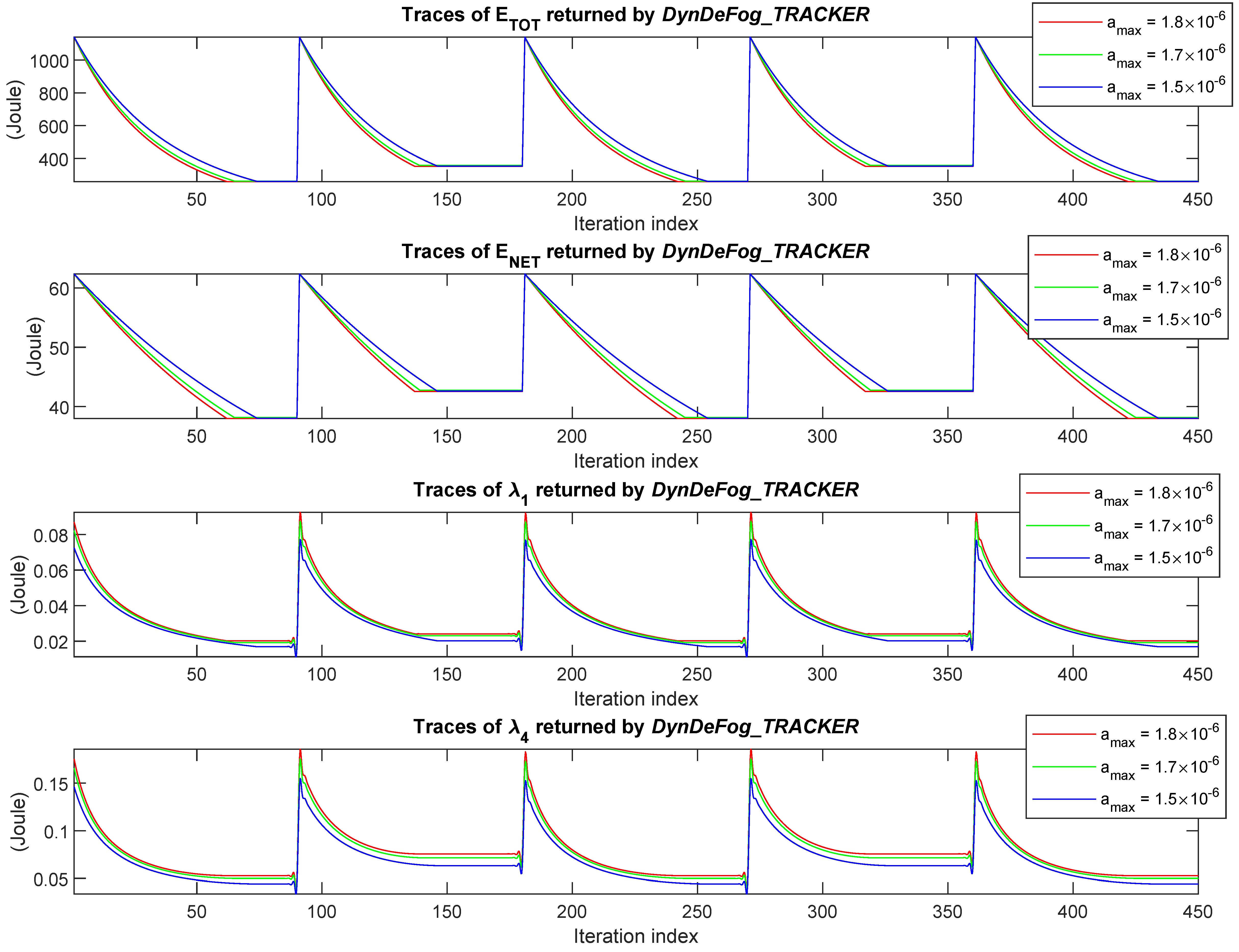
The first scenario, presented in Figure 15, refer to the case in which Fog$(1,3)$ and Fog$(2,3)$ nodes sequentially fail under $T2$ topology. This figure illustrates the obtained dynamic behaviors of the total and networking energy ${\mathcal{E}}_{TOT}^{\left(best\right)}$ and ${\mathcal{E}}_{NET}^{\left(best\right)}$, as well as the Lagrange multipliers ${\lambda }_1$ and ${\lambda }_4$ associated to the first and last constraints on the inference times in (23b). Figure 15 shows that increasing values of the $a_{MAX}$ clipping factor speed-up the convergence of Algorithm 1 and the Fog platform of Figure 3 self-adapts its resources in within 70 iterations (see the third and fourth plots in Figure 15). In addition, we can argue that the tracking behavior is robust to the settings of the $a_{MAX}$ parameter, so that the resulting technological platform of Figure 3 is capable of self-react and promptly adapt to abrupt failures of some of FNs composing the execution platform within a broad range of values of the $a_{MAX}$ clipping factor. A careful examination of the second and fourth tracts of the curves of Figure 15 (i.e., the index intervals 90–180 and 270–360) shows that the energy assumes the same steady-state values. This behavior is justified by the symmetry of the considered topology after failure events. In fact, in both the segments, the failure event involves one of the two FNs located at $tier\#3$ of $T2$ in Figure 8 that share the same values of the underlying resources. In both cases, after the failure, $tier\#3$ remains with a single active FN, and then it consumes the same energy.

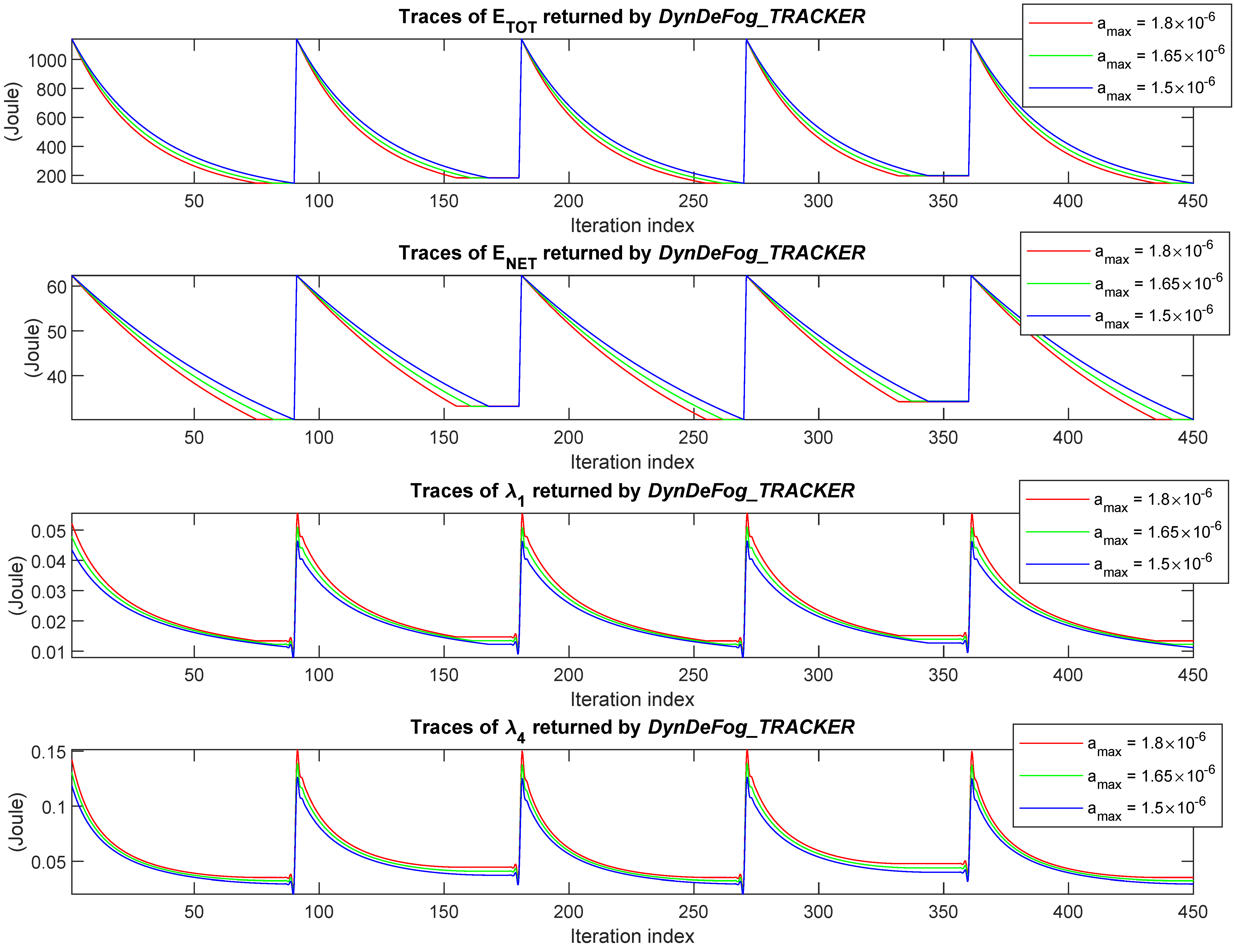
Finally, the second scenario featured by Figure 16 refers to the case in which Fog$(1,3)$ and Fog$(4,2)$ nodes of the topology $T2$ sequentially fail. This figure suggests a convergence behavior similar to the previous scenario, and once again the platform is capable of automatically and promptly adapting its resource allocation for coping with the experienced failure event. However, in this case, differently from the first scenario, the failures involve nodes located at different tiers of the $T2$ topology, and this gives rise to asymmetric steady-state behaviors. In fact, a careful examination of the curves in Figure 16, specifically in the second and fourth tracts (i.e., over the index intervals 90–180 and 270–360), shows that the steady-state energy assumes different values. Specifically, the total energy ${\mathcal{E}}_{TOT}^{\left(best\right)}$ after the failure of Fog$(4,2)$ is about 17 (Joule) greater than the corresponding one after the failure of Fog$(1,3)$. This behavior is justified by both the convexity of the energy model introduced in Section 4 and the fact that the workload to be processed at each tier reduces going up in the topology, towards the Cloud node, since a considerable fraction of the workload undergone early exits. This observation implies, in turn, that the failure of FNs at lower tiers (such as Fog$(4,2)$) causes a greater energy consumption than the failure of FNs at higher tiers (such as Fog$(1,3)$).

To summarize, the proposed DeepFogSim toolkit can be considered as an effective software tool for simulating and testing the energy-vs.-delay performance of the technological Fog platform supporting the distributed execution of the inference phase of CDNNs with early exits.

8. Conclusions and Hints for Future Research

It is expected that the convergence of Conditional Deep Neural Networks, Fog Computing and IoT allows the energy-efficient and real-time distributed mining of big volumes of data generated by resource-limited sensing devices, possibly scattered over large geographically areas. Motivated by this expectation, in this paper, we present DeepFogSim, a MATLAB-supported software toolbox aiming at simulating and testing the performance of Fog-based technological platforms supporting the real-time execution of the inference phase of CDNNs with early exits. The DeepFogSim toolkit provides a new software environment that accounts for the main system parameters featuring the computing and network aspects of the underlying Fog-Cloud execution platforms. The core engine of the DeepFogSim toolbox allows the optimized allocation, simulation, and tracking of the computing-plus-networking resources wasted by the dynamic execution of the inference phase of CDNNs with early exits under hard constraints on the allowed per-exit inference delays. The GUI equipping the DeepFogSim package allows a user-friendly rendering of the simulated data under a number of easy-to-understand graphic formats.

The current version of the DeepFogSim package could be extended along four main directions. First at all, the stack topology the considered CDNNs with early exits of Figure 1a could be augmented by inter-layer feedback connections, so as to give rise to recurrent-type CDNNs which are capable of exploiting the time correlations possibly present in some IoT input streams, such as those typically featuring video/audio sequences, as well as multi-view scenes, to name just a few. Second, the networking energy models of Section 4 can be extended by accounting of the effects of spatial coding and multiplexing [46,47] operating over Terahertz communication channels, in order to exploit a massive number of terminal antennas as envisioned by the future 6G communication paradigm [2]. Third, suitable algorithms for the forecast of the inter-tier network traffic and the automatic start/stop of the carried out iterations of Equations (24) and (25) could be introduced, in order to allow the simulated platform of Figure 3 to cope with failure events in a pro-active (instead of re-active) way. Finally, new functions could be introduced in the current version of the DeepFogSim toolkit, in order to simulate the effects of inter-thing social relationships, such as those featuring the emerging paradigm of the so-called Social IoT (SIoT) [48].

9. Availability of the DeepFogSim Package

The full software package of the DeepFogSim simulator and the corresponding User Guide are downloadable for free on the GitHub repository site at: https://github.com/mscarpiniti/DeepFogSim. In addition, access to the software package is provided on the authors’ academic web pages.