From Electricity and Water Consumption Data to Information on Office Occupancy: A Supervised and Unsupervised Data Mining Approach


1
Department of Mechanical Engineering, Aalto University, 02150 Espoo, Finland
2
Innovation and Development, Granlund Oy, 00701 Helsinki, Finland
3
College of Urban Construction, Nanjing Tech University, Nanjing 211800, China
*
Author to whom correspondence should be addressed.
Appl. Sci. 2020, 10(24), 9089; https://doi.org/10.3390/app10249089
Submission received: 4 November 2020
/
Revised: 2 December 2020
/
Accepted: 16 December 2020
/
Published: 18 December 2020
(This article belongs to the Special Issue High Performing Heating, Ventilation and Air Conditioning (HVAC) Systems to Provide Excellent Indoor Climate in Energy Efficient Manner)
Abstract
:Climate change and technological development are pushing buildings to become more sophisticated. The installation of modern building automation systems, smart meters, and IoT devices is increasing the amount of available building operational data. The common term for this kind of building is a smart building but producing large amounts of raw data does not automatically offer intelligence that would offer new insights to the building’s operation. Smart meters are mainly used only for tracking the energy or water consumption in the building. On the other hand, building occupancy is usually not monitored in the building at all, even though it is one of the main influencing factors of consumption and indoor climate parameters. This paper is bringing the true smart building closer to practice by using machine learning methods with sub-metered electricity and water consumptions to predict the building occupancy. In the first approach, the number of occupants was predicted in an office floor using a supervised data mining method Random Forest. The model performed the best with the use of all predictors available, while from individual predictors, the sub-metered electricity used for office equipment showed the best performance. Since the supervised approach requires the continuous long-term collection of ground truth reference data (between one to three months, by this study), an unsupervised data mining method k-means clustering was tested in the second approach. With the unsupervised method, this study was able to predict the level of occupancy in a day as zero, medium, or high in a case study office floor using the equipment electricity consumption.
1. Introduction
Buildings are responsible for approximately 36% of all CO2 emissions in the European Union and 28% on the global level. Therefore, the EU has set the goal of developing a sustainable, competitive, secure, and decarbonised energy system by the year 2050 [1,2]. One of the ways of achieving this goal is through the digitalisation of energy systems and buildings. The EU expects that smart-ready energy systems and buildings are going to offer new opportunities for energy savings. In order to promote smart ready technologies for the building sector, the EU has introduced a smart readiness indicator (SRI). The purpose of SRI is to determine the capability of buildings in using the information and communication technologies to adapt the building operation to the needs of the occupants and the grid while improving the overall performance of the building [1].
Efforts of increasing the building smartness will also increase the number of sensors in buildings, which will, as aresult, create massive amounts of building operational data. Processing and combining this data further can increase its value by providing new knowledge [3]. For instance, building operational data is reflecting the interaction between occupants [4,5], the building (with its systems) and the environment. The outdoor and indoor environment, the building’s energy consumption and the system operation are usually monitored with sensors and meters, but the occupancy pattern and behaviour are not. Collected data processed using data mining techniques can provide information about building occupancy. Understanding the occupancy dynamics of the building, with other previously mentioned building variables creates knowledge that can be used for tasks such as energy, space and facility management, or even as an aid to the organisation’s human resources department. For example, in the field of building simulation, occupant behaviour was recognised as a significant factor contributing to the high discrepancy between simulation prediction and real energy use [5,6,7,8]. Furthermore, Tianzhen et al. [9] have listed ten challenges of building simulations where information on occupancy schedule is directly affecting three of them (addressing the building performance gap, modelling human-building interactions and energy model calibration).
Data mining is defined as “the process of discovering insightful, interesting, and novel patterns, as well as descriptive, understandable, and predictive models from large-scale data” [10]. Data mining is a multi-disciplinary subject that combines methods from statistics, machine learning and artificial intelligence. It can be divided into two distinct groups: supervised and unsupervised analysis. The supervised analysis is the one that uses a training dataset in which both input and output variables are available. By using regression or classification algorithms, the supervised analysis describes quantitative or qualitative relationships between input and output variables. After the supervised model was developed (trained) on training data, it can be applied to a new dataset, containing only inputs while predicting the output data. On the other hand, unsupervised analysis is done on a dataset that includes only inputs, while the target is unknown. It focuses on exploring the correlations, associations, and patterns in the dataset, and in that way, unsupervised analysis can discover new knowledge [11].
Using building operational data with both supervised and unsupervised data mining methods to find more information on occupancy and its influence on building operation, has already been part of various studies, e.g., Kleiminger et al. [12], Mora et al. [13], Yang, L. et al. [14]. Building operational data used in those studies was typically electricity usage, measured occupancy or indoor climate measurements. Information being discovered in those studies was ranging from grouping buildings or consumers by their energy usage, finding occupancy and consumption patterns or detecting and predicting the occupancy in buildings.
In a study by Kleiminger et al. [12], supervised data mining methods were used to determine the occupancy presence on the smart meter data from five Swiss households during a period of eight months. The ground truth of the occupancy was acquired using the application on the tablet computer. Supervised methods used in this study were classification algorithms such as Support Vector Machines (SVM), K-nearest neighbour (KNN), thresholding (THR) and the Hidden Markov Model (HMM). Results from this work have shown that it is possible to achieve occupancy detection accuracies of over 80% from smart meters in households. Improving on this work, Kleiminger et al. [15] have managed to achieve average occupancy detection of up to 94% by introducing dimensionality reduction and extending the feature set and the set of classifiers. Yang, L. et al. [14] have worked on inferring occupancy in a university laboratory using smart meter data. Their work has tried to infer binary occupancy status (present, not present) and ranged occupancy (range of the number of present occupants). Since in the lab, the maximum occupancy is twelve persons, the authors have divided occupancy into four bins (0, 1–2, 3–5, 6–12). Authors have used the following classifiers: NaiveBayes, Random Forest, Decision Tree, Multilayer Perceptron and KNN. Results from this work have shown that it is possible to infer binary occupancy status and range with high accuracy and that the best classifiers have shown to be Multilayer Perceptron and Random Forest. Interestingly, the authors have experimented with the training set size and found that the best size was 8 days, while shorter or longer training set sizes increased the error.
Supervised data mining was also used for detecting the occupancy on a workstation level in the office. Akbar et al. [16] used different features from data collected by smart electricity meters, which were installed on four employees’ workstations. Classifiers analysed in the study were KNN and SVM. Overall, results from the study have shown that the KNN classifier performed the best, with the occupancy status detection accuracy of up to 94%. Studies that used supervised methods for occupancy detection from smart meter data were not only done on small scale. In a study by Razavi et al. [17], occupancy detection in residential buildings was performed on the dataset from 5000 buildings. Classification methods were Random Forest, SVM, KNN, neural network (NN) and gradient boosting. This work has shown that it is possible to detect occupancy in households with high accuracy even by using a big dataset. Furthermore, the authors have shown that classifiers could generalise very well across different households, which makes this technology highly scalable. Reviewed studies that used supervised data mining on smart meter data have all commonly been done with a goal to detect occupancy or at the best to determine the range of occupancy and most of them were targeting households. Furthermore, the dataset with high sampling frequency was used where electricity consumption was measured by every second.
In recent years, unsupervised data mining methods, such as clustering, have been applied to building operational data in various studies. These methods have shown some encouraging results even though their applications are still at an early stage [11]. Earlier studies in the field primarily using clustering were trying to find patterns in the energy consumption on a larger scale (district or even a country level) and/or to group the consumers. Such studies have used electricity usage data from a large number of Chinese, Irish or American households to create residential electricity profiles to which consumers have been grouped and classified by their social status [18,19,20]. In a study by Yang et al. [21], clustering was used on energy consumption from 10 institutional buildings to improve the building energy consumption forecasting.
Following the studies on the larger scale, clustering has been emerging on the building level, where the energy consumption from one or several buildings has been clustered for finding either occupancy energy usage patterns or the actual occupancy patterns. In a study by D’Oca and Hong [22], the k-means clustering algorithm has helped the authors to determine the number of typical occupancy patterns in a presence dataset from 16 single office rooms. While centroids of those clusters were used to create occupancy profiles, which could be used as an input to the building performance simulation. A similar study, but on a larger scale of the whole building, was done by Liang et al. [23] where k-means clustering was used to find the occupancy patterns, while profiles were created using the Decision Tree supervised method. Authors have managed to create the occupancy profiles and predict their occurrence using time of day, weekday and season. The highest uncertainty in the occupancy profiles prediction has shown to be at the start and end hours of the working day.
Another work, where the aim was creating inputs for building simulation was done by Causone et al. [24]. They have proposed a data-driven approach for modelling of occupancy and occupancy-related electric load profiles. They have used a two-step clustering approach with k-means and Self-Organising Map (SOM) to find patterns in electricity data from households, which k-NN algorithm used to create a yearlong profile. The occupancy presence profile was created from electricity consumption with the method from the previously mentioned work of Kleiminger et al. [12,15].
So far, the mentioned research has mostly tried to find patterns in a particular variable by clustering that same variable. The attempt to find the pattern of an unknown variable by clustering known and correlated variables could bring additional value to existing data in the building. This could be beneficial for finding occupancy patterns of buildings since occupancy is rarely measured in the buildings because it is difficult to measure. Mora et al. [13] have done this by applying the clustering on the variables which significantly correlate with the occupancy, such as CO2 concentration, electric power, room air temperature, humidity, air conditioning operation mode and window opening status. The authors have used these variables with hierarchical clustering to identify the occupancy patterns of a single person office. Clusters of measured variables by the time of day were then compared with the ground truth clusters. The analysis has shown that using electricity consumption was a good predictor for the occupancy state during morning and afternoon while CO2 was also a good predictor during lunchtime. They have shown that it is possible to use commonly measured variables such as CO2 concentration and electricity consumption to predict the occupancy patterns of a single person room. On the other hand, the proposed method requires much effort to be used for identifying the occupancy patterns of just a single room, which makes the scalability of the method difficult in practice.
The analysis of the literature highlights the potential that building operation data has with the data mining methods. Studies that used supervised data mining methods with smart metering data have proven that it is possible to detect occupancy presence or its range, mostly in residential and in some small-scale office environments. Other studies that used unsupervised methods managed to group the consumers by their consumption patterns, or they successfully created the occupancy or occupancy-related electric load profiles from the historical measurements of the same values. Mora et al. [13] have shown that it is possible to use the unsupervised method on a measured variable and find the information about the correlated but unknown variable.
This has all led to the development of this study, where the novelty is using a commonly measured variable such as sub-metered electricity or water consumptions to acquire the information on the occupancy from a larger area, such as office building floor. This is done with two different data mining approaches by using supervised and unsupervised methods. By using a supervised data mining method, the possibility of predicting the number of occupants on the office floor is assessed. For the training of the supervised methods, the long-term continuous and costly ground truth collection of the actual occupancy is needed. This has been detected as one of the challenges of occupancy prediction technologies by Dong et al. [25,26] as well. Following-on this, the unsupervised data mining method of consumption data to find daily occupancy level is evaluated. The additional novelty of this study is using the dataset with the sampling time of one-hour, which is more common in energy reporting tools than the high-frequency datasets used in many of the reviewed studies.
2. Methodology
2.1. Case Study
2.1.1. The Building
The building serving as a case study in this work was an office building of a consultancy company in Helsinki, Finland. The building with four floors above the ground was built in 1990. The total occupied floor area was 9672 m2. The focus of the study was the third floor, which had an area of 1900 m2 and can be seen in Figure 1. The layout of the third floor was a typical open-office layout with 16 meeting rooms. The selected floor was the company’s representative floor, and it regularly received visits from the company’s clients who attended meetings. The employees could work remotely, which meant that many of them were not in the office every day. All previous factors affected the floor occupancy significantly and made it difficult to predict.
2.1.2. Electricity Sub-Metering
An extensive network of electrical energy consumption sub-metering is installed in the building, where there are dedicated meters for different zones and also for different sub-systems of building service systems (cooling system, ventilation, etc.). The data used in this study were collected with meters measuring the power consumed by the lighting system and the equipment connected via sockets in the office. For these two categories of electricity consumption, occupants have a direct impact. Most of the lights on the floor are workstation-based and are occupant operated, so the assumption was that lighting electricity has a good correlation with occupancy. The same goes with the equipment electricity consumption, where most of the devices connected were personal computers; desktop and laptops. Both desktops and laptops were connected to either one or two computer screens.
The floor consisted of three wings which had their own sub-meters for lighting and equipment. The consumptions of each zone were combined into floor-level consumptions in order to be comparable with available ground truth occupancy.
2.1.3. Water Consumption
Water consumption was measured on an hourly basis by the central water meter for the building. For this study, the assumption was that water consumption in the office building was equally distributed on three floors since all floors were similar. By using this assumption, it was possible to estimate target floor water consumption on the studied floor.
2.1.4. Ground Truth
Assessing the accuracy of the machine learning algorithms requires information on the occupancy of the floor. For the supervised method, this so-called ground truth is not only crucial for the model assessment but also training of the model. Cameras installed on the four entrances to the floor were installed to measure ground truth in this study. These cameras were equipped with people counting software which reported the number of people entering and exiting the floor.
Commercial people counters, such as the ones used in this study, are not accurate enough to give absolute truth [27]. In some instances, it happens that counters undercount, especially when several persons pass under the camera at the same time. When calculating the occupancy from the people counts, this error was visible at the end of the day when it seemed that some persons had not left the floor. The error at late night hours was not crucial, since this study focused on the regular working hours. Additionally, occupancy calculation was reset to zero each day at midnight. An alternative would be manual people counting, which would be very difficult to perform hourly throughout every hour of seven months on four entrances. Therefore for this study, where the development of the method of high accuracy was not the goal, it was decided to accept this error.
2.2. Supervised Method—Random Forest
The supervised method applied in this work was the Random Forest, a popular machine learning algorithm. The Random Forest was chosen because it has been already successfully applied in some of the reviewed studies in the introduction section, where it has shown good performance, and it is easy to implement.
The Random Forest algorithm is based on a Decision Tree algorithm, where data is split into nodes forming a tree based on rules, such as if-then-else rules. A combination of many of these trees makes a Random Forest. The word random comes from the way the algorithm creates new nodes, by randomly selecting predictors. This is unlike the ordinary Decision Tree, where each node is split using the best split among all predictors. The new data is predicted by using the predictions made by all trees in the Random Forest, where a majority vote is used for classification, while the average prediction is used for regression [28]. In this work, the Random Forest regression algorithm was used, since the used variables are continuous.
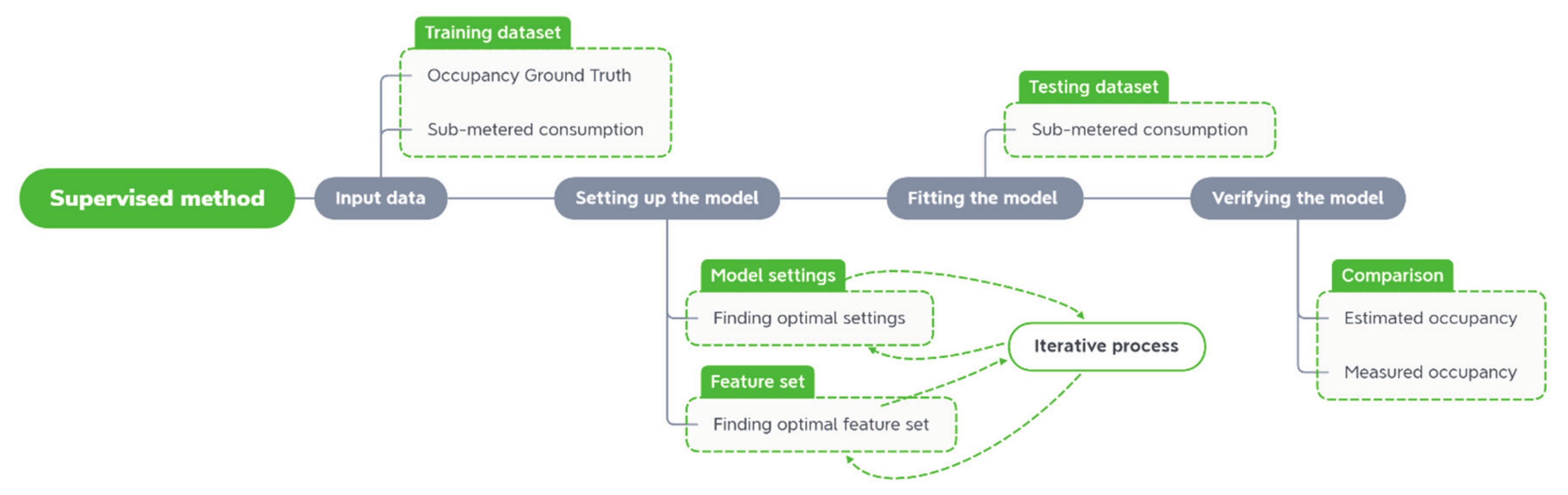
The Random Forest was applied with Python module Scikit-learn, which is a general-purpose, high-level programming language for machine learning [29]. A dataset with predictors and occupancy ground truth was split into training and testing periods and an iterative process of determining settings for the Random Forest algorithm was done. This iterative process was done by minimising the error between predicted and measured occupancy, while at the same time keeping the computational time low. The whole process of the supervised data mining approach for predicting the number of occupants in the office is presented in Figure 2. After the model was set up with the training dataset, the model was fitted on a testing dataset, giving the occupancy prediction. Finally, this prediction was assessed with the measured occupancy using the error metrics, which are described in the following section.
Error Metrics for the Supervised Method
The following error metrics were used for verifying the results of the supervised method: explained variation, root mean square error (RMSE) and mean biased error (MBE).
Explained variation (percentage of) is a variable that shows the relative goodness of prediction. Variance expresses how spread the values of a particular variable are, while explained variance shows how much of that variance is explainable by predictor variables. A model that would make perfect predictions would have an explained variation of 100%.
RMSE, on the other hand, is an absolute measure of the fit (expressed in units of predictions) that shows explicitly how much predictions deviate, on average, from the actual values in the dataset. Furthermore, RMSE additionally “punishes” more significant outliers, because of the square in the RMSE equation.
The third metric in the paper, MBE, is, together with the RMSE, the most commonly used error metric in the analysis of prediction models. MBE gives information about the average deviation from the mean of the testing dataset. Unlike RMSE, MBE keeps the sign of the error which means it gives information about over- and under- predictions. On the other hand, a series of variations higher or lower than the predicted values generates a small MBE, whereas the real competence of the model can be low. Since each metric has its own issues, in this work we used their combination to assess the different predictors.
2.3. Unsupervised Method—The k-Means Clustering
For the unsupervised part of this study, clustering was used, which is the task of organising a given set of unlabelled data objects to specific clusters (groups). Since clustering works with unlabelled data, ground truth data is not needed for training of the model, but in this work, measured occupancy was used for the verification of the results. The clustering method chosen for this work was k-means, which is one of the most popular clustering methods and it has been widely used for the clustering of raw datasets in the energy and built environment field and some of them have been reviewed in the introduction section.
The k-means algorithm requires a predefined number of clusters, k, in which data samples, or for this study day profiles, were placed. The algorithm uses the iterative scheme, where it first randomly selects the initial cluster centres around which it distributes the data samples. Then, cluster centres and the distribution of data samples are updated until the value of the objective function reaches a minimum [30]. To achieve the clustering process, the similarity of the data needs to be measured, which can be more difficult with the time-series data. In time-series, not only the magnitude of data points needs to be considered, but also the order of data points in the sequence. Traditionally with k-means, the Euclidean distance metric has been used as a similarity measure, but regarding time-series data, this measure is not accurate. A similarity measure that was developed explicitly for time-series is dynamic time warping (DTW) [31]. Given this similarity measure, clustering algorithms such as k-means also need an averaging method to be able to describe clusters that they form (cluster centres). The method used for averaging of time series in this work was dynamic time warping barycenter averaging (DBA) [32].
The k-means algorithm used in this work was tslearn, which is a Python package that provides machine learning tools for time-series analysis [33]. The main parameter which needs to be set for the k-means algorithm is k, the number of clusters. For this, the Elbow method was used, developed by Thorndike [34]. The idea of the Elbow method is to calculate the k-means algorithm with the range of values for the k. For each value of k, the distortion score was calculated, the sum of square distances from each point to its assigned centre. With a plotted distortion score for each of the k, it was possible to visually determine the best value for k. The best value was the one located at the “elbow” of the curve (the point of the inflection on the curve). Detecting the “elbow” curve was done using the elbow detection algorithm (the kneedle), which finds a point of maximum curvature. The algorithm was developed by Satopää et al. [35], and in this work was applied using the Python package Yellowbrick [36].
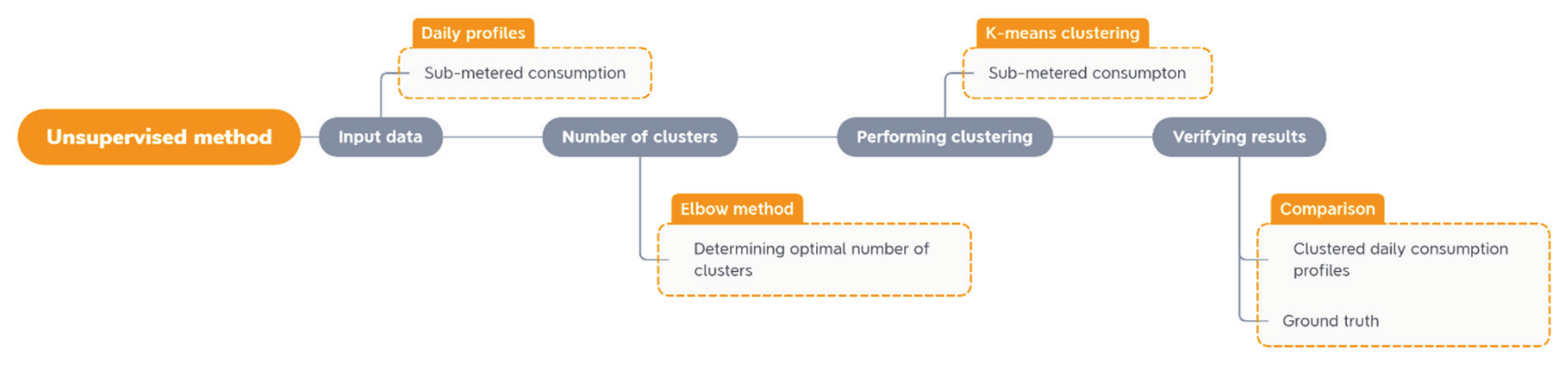
A summary of the unsupervised method is presented in Figure 3. It shows the selection of the optimal number of clusters as a step before the main clustering and finally, the verification of the whole process with the ground truth.
3. Results
3.1. Data Gathering and Processing
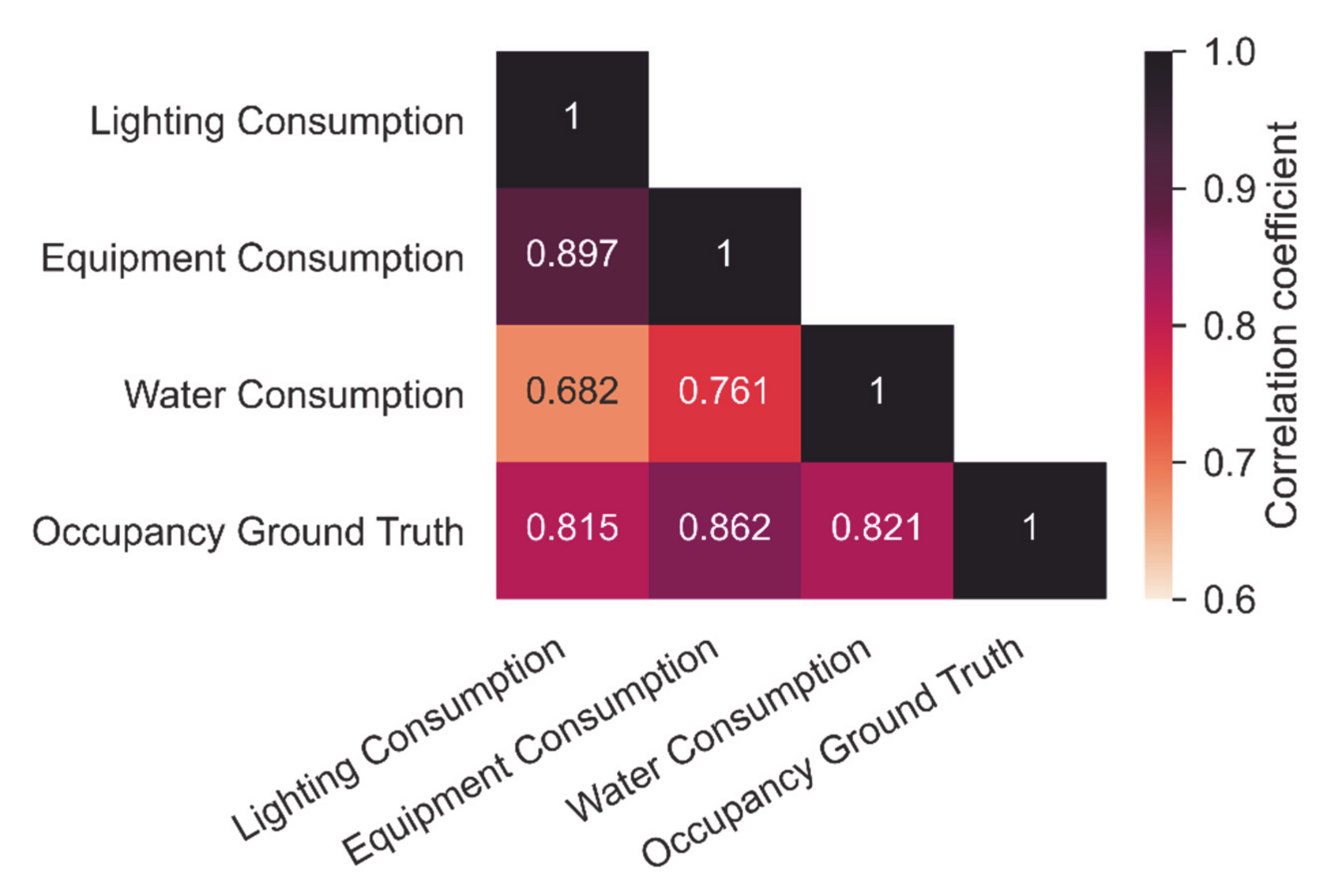
Data gathering of the electricity and water consumption data was done by using Granlund Manager [37], a facility management software to which smart metered data was stored. The facility management software obtained data from the building management system and the utility companies in the hourly interval. Electricity data was collected in kilowatt-hours consumed, and water in cubic meters consumed. For this work, measured electricity consumption for equipment and the lighting was used on the case study floor. Additionally, for the supervised study, a sum of both sub-metered electricity consumptions as a variable called total sub-metered electricity was used as well. Ground truth data on the occupancy was collected from the camera with people counting software in 30-min intervals, which was summed to hourly intervals so that it could be compared with the consumption dataset. In Figure 4, the correlation matrix shows that selected predictors had a very good correlation with the ground truth of which equipment electricity consumption had the highest.
The acquired dataset was for the period between the 1st of February and 31st of August 2017. Before analytics was performed, the dataset had to be cleaned. First, the weekends were taken out of the dataset, since the floor was very rarely occupied during weekends. This was decided since weekend occupancy is sporadic and occupant type was often different than during the week. It was more common that cleaning, maintenance or security personnel passed through the building than the regular company employees. Different occupant types used electricity and water in a different pattern than the regular occupant, which decreased the model performance. Second, since there were no occupants on the floor during night time, it was decided to use only the data between 06:00 and 21:00.
Additionally, the water meter had missing data during some days, and those days were removed from the dataset. Dataset processed in this way was used in both supervised and unsupervised methods of this paper.
3.2. Results of the Supervised Method
The supervised method based on the machine learning algorithm Random Forest was applied to the dataset processed as previously explained. The iterative procedure of setting up the model was performed, where the model slowly stopped improving when it had more than 500 predictors. Since this model on this dataset was not computationally expensive, it was decided that the calculation would be done with 1000 predictors.
3.2.1. Selection of Features
The dataset contained collected raw data, and extracting additional features from the data could improve the prediction model. Table 1 describes the extracted features used in this study. First and second-order difference (FD, SD) captured temporal variations, while the moving average (MA1, MA2) took into account the time delay between parameters.
Having these features available in the dataset did not necessarily improve the model, while it increased the computational time. Therefore, an iterative study to pick the right features for every set of predictors was performed. For every set of predictors, the Random Forest regression algorithm was applied with different combinations of features FD, SD, MA1, MA2, hour, weekday and month, including all of them, some or none. The combination which had the lowest error was chosen as the final. In Table 2, chosen combinations can be seen, where the letter in subscript notates from which parameter the feature was calculated (L—lighting, E—equipment, W—water, T—total).
3.2.2. Data Analysis and Results
In this section, the results of the supervised method for occupancy rate prediction for the test period (15th to 31st of August 2017) are presented. The last half of the month August was selected for testing as it was at the end of the available dataset, while the earlier period was used for model training. Weeks before the testing period was usually a period when employees took their summer vacation (from July to early August). Using the vacation weeks as a testing dataset for a model trained on more regular working periods would not give representative results. Another possibility was to shuffle the dataset and use other earlier periods, but using future data to predict history is questionable when dealing with time-series data [38]. However, data sufficiency and generalization analysis in Section 3.2.3. explore different training dataset lengths and testing periods.
Each set of predictors with the previously mentioned selected features is presented in Table 3 with error indices. Results show that All predictors have the best result, when looking at the RMSE and explained variation, with slight underprediction, which is shown with a negative MBE value. Light and equipment are showing the second-best results, but with higher underprediction. Total floor electricity consumption shows the lowest absolute MBE value, while the value being positive means that the model using this predictor usually overpredicts. Surprisingly, Water consumption was shown to be a better predictor than Lighting consumption, which was shown as the worst. This confirmed the predictor ranking seen from the correlation matrix (Figure 4). Regarding the explained variation, all results were above 90%, which meant that the models had a good prediction capability where even the model with the Lighting consumption predictor, still showed an average explained variation of 93%.
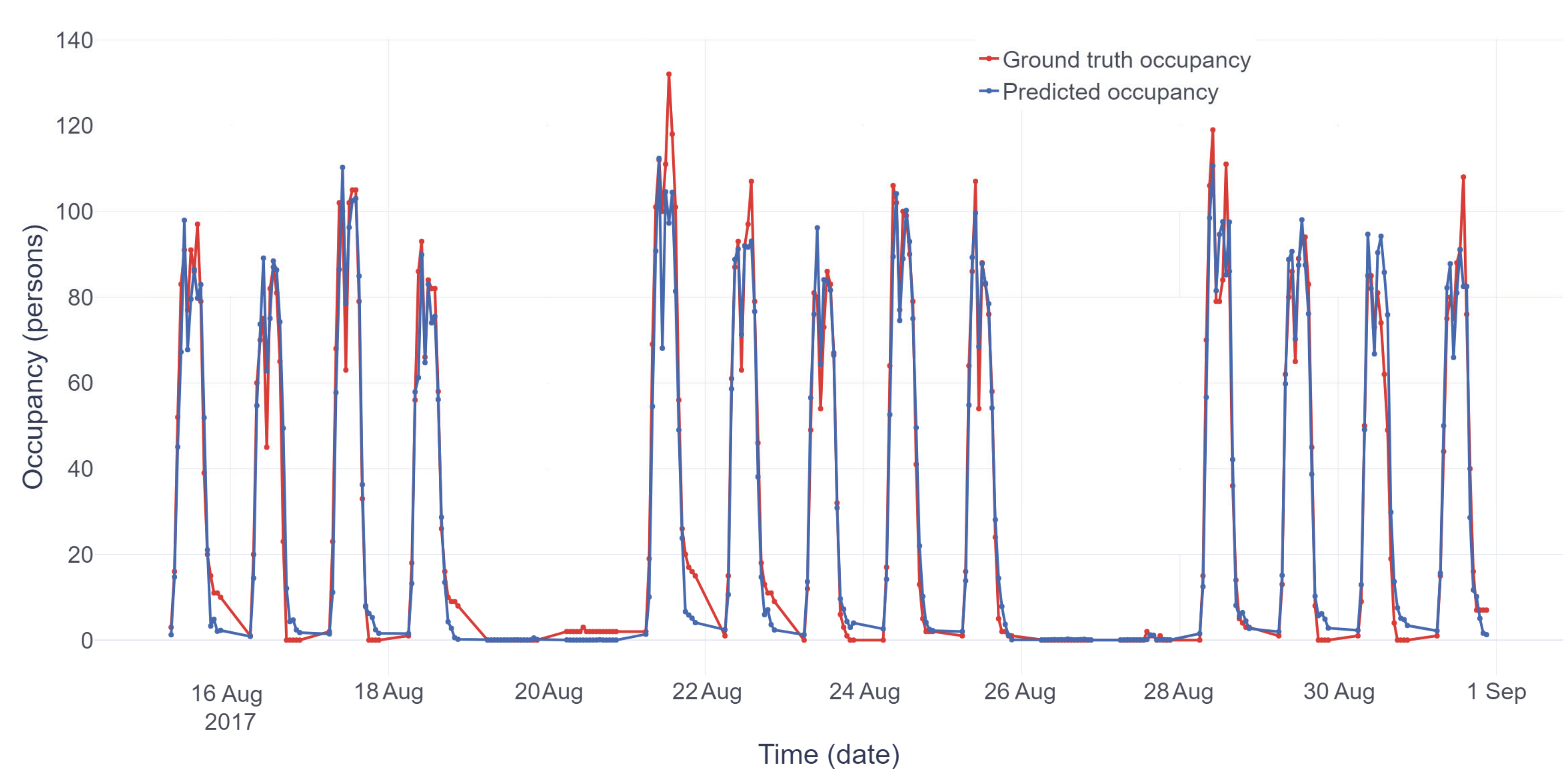
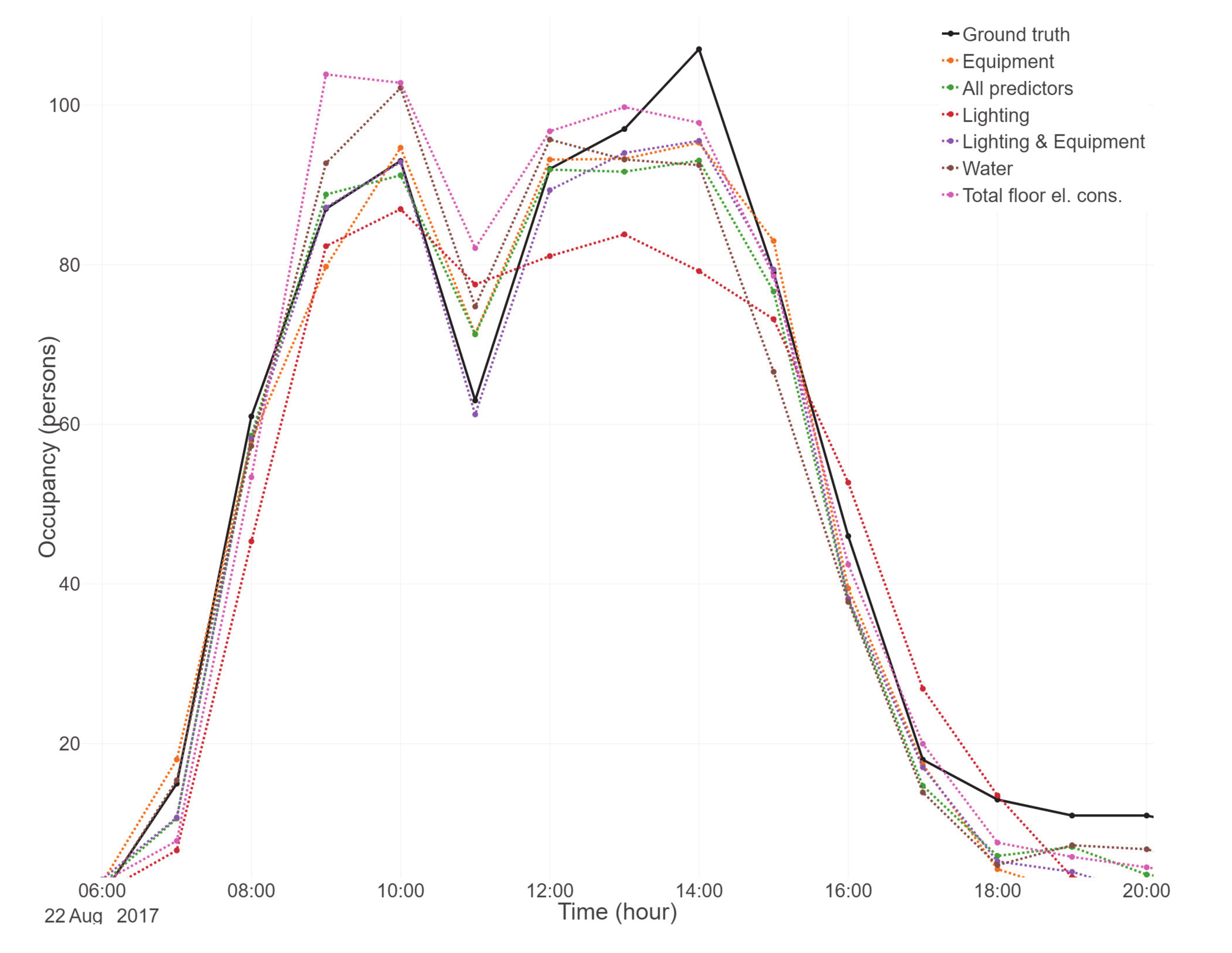
Comparison between ground truth occupancy and predicted occupancy using the best performing model (all predictors) is shown in Figure 5 for the test period. It is possible to see that predicted occupancy was following quite well with the ground truth occupancy and that the most considerable difference between the predicted and ground truth mostly happened during peak hours. During peak hours usually, there was a number of external visitors participating in meetings, which were less likely to consume additional energy for equipment or lighting.
The performance of the models with different predictors can be seen in more detail in Figure 6, where they can be closely compared with ground truth data for a randomly selected day from the testing period. For this day, the model which used lighting as its predictor showed significant underprediction during peak hours, while total floor electricity consumption showed overprediction, especially at 9 o’clock.
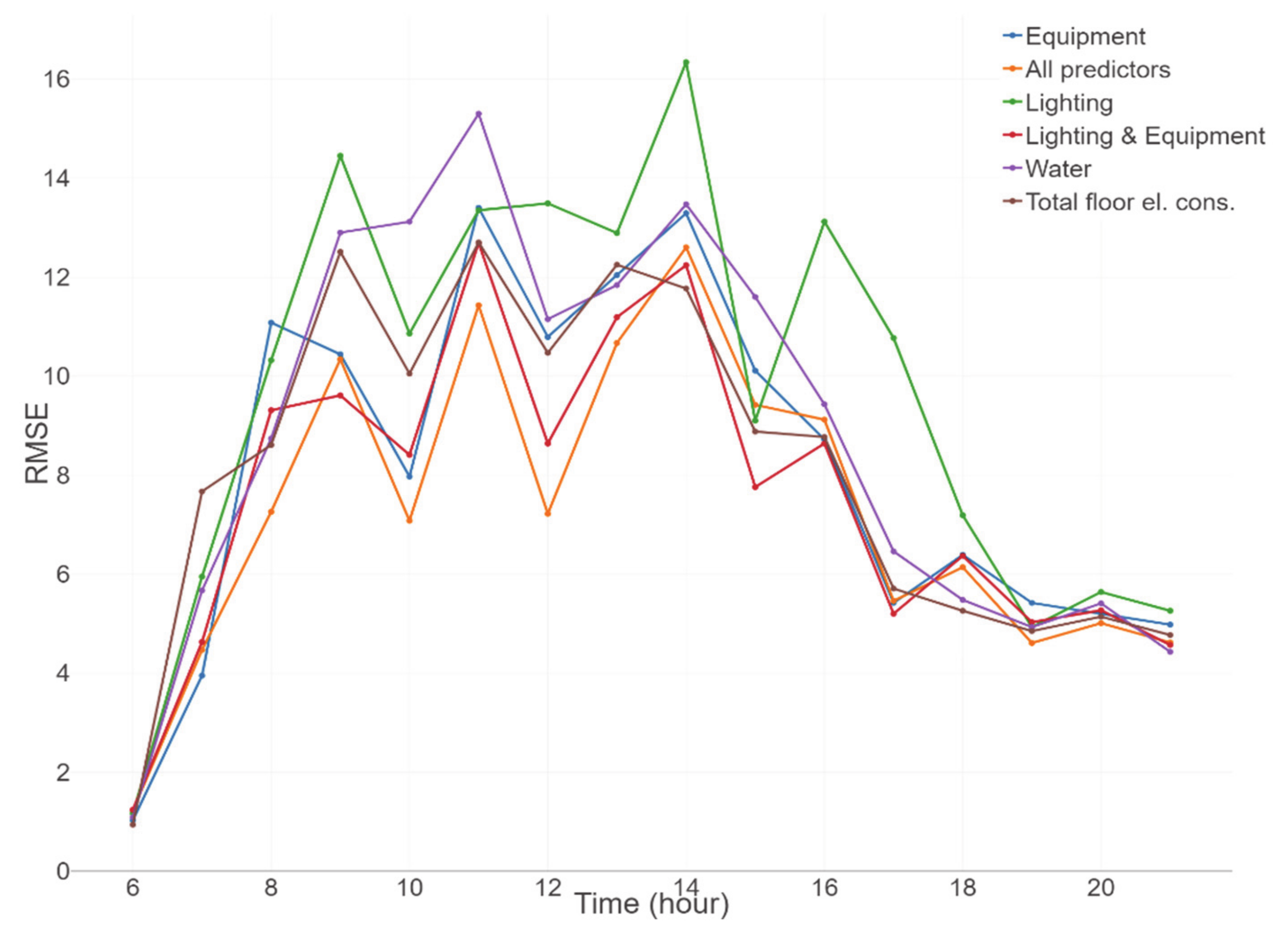
In Figure 7, RMSE is shown for every hour of the testing period. It can be seen that using lighting consumption as a predictor created a larger error in the second half of a workday. This could be explained by employees turning the lights on later in the day or forgetting to turn them off when leaving the office. At 18 o’clock, the error from the model with lighting consumption predictor decreased, most likely because of the scheduled corridor lights being shut down. On the other hand, the model which used water consumption as a predictor showed a significant performance gap, compared to other predictors, around 11 o’clock, which was the usual time for employees to visit the office canteen.
Interestingly, from 19 o’clock, the RMSE value showed a nearly constant and similar value between all predictors. The reason for this was the issue with the method of collecting ground truth data, which was explained in Section 2.1.4. This issue is also visible in Figure 5 and Figure 6, where the ground truth does not reach zero occupancies at the end of the day. Moreover, the assumption was that there was nobody in the office during those hours.
3.2.3. Data Sufficiency Analysis and Generalisation Analysis
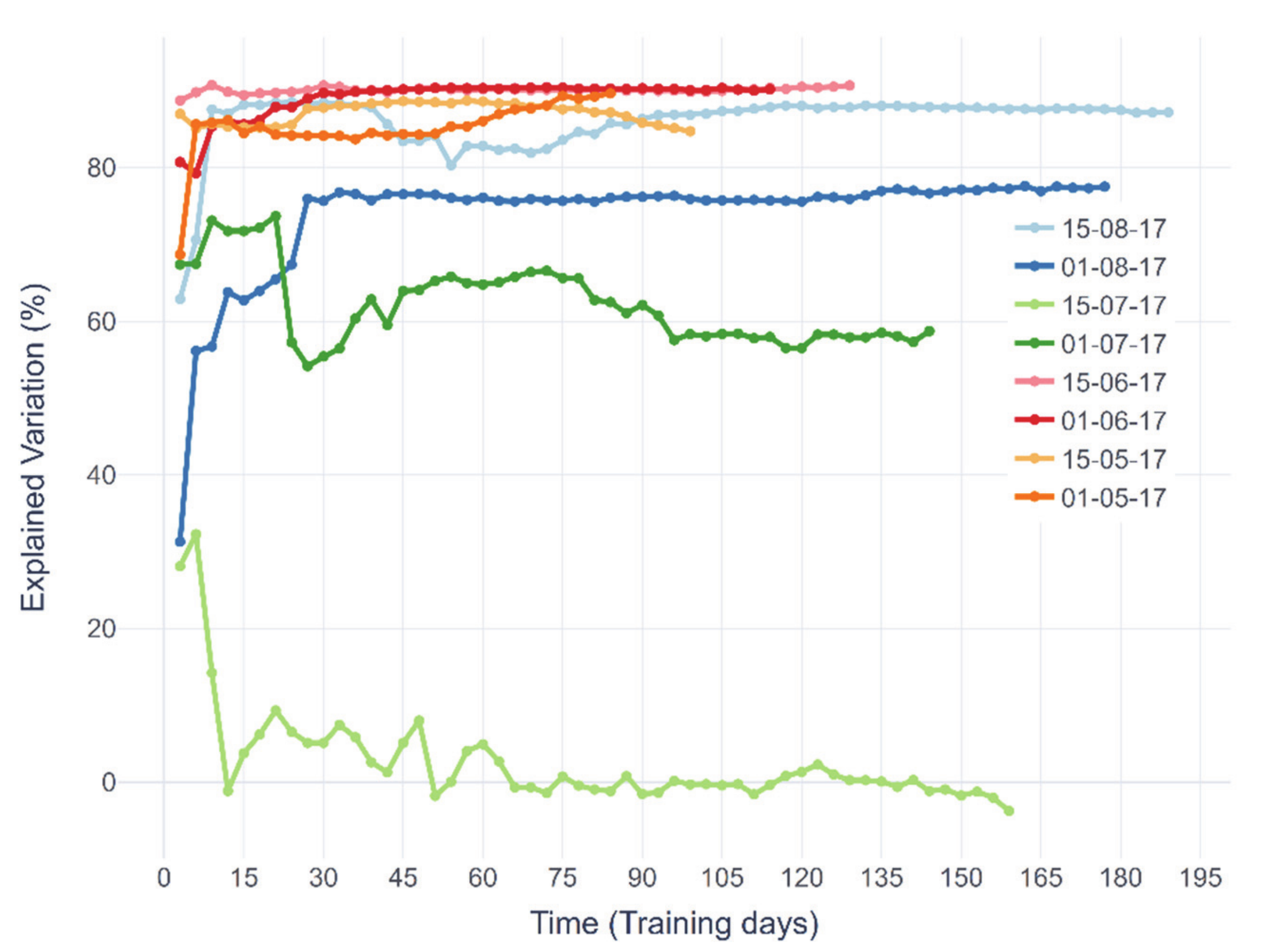
In the previous section, the results of predicting occupancy from consumption using the model based on the Random Forest algorithm have been shown. Since those results came from a single testing period, which was chosen to be the last half of the month in the dataset, additional verification was done by applying the algorithm during other periods from the dataset and with different training lengths. For this purpose, half a month of testing periods were selected, starting from the 1st of May until the 31st of August. Model training period length was varied from three days before the testing period until the beginning of the dataset by three-day steps.
Occupancy prediction errors were calculated, as RMSE and EV, for these eight testing periods and are presented in Figure 8 and Figure 9. In these figures, each line represents the occupancy prediction error for a single testing period dependent on the length of model training. First, it can be seen that during vacation time (two testing periods in July), the lowest EV values were shown, because of that period being untypical compared to its training dataset. On the other hand, the lowest RMSE value during the July period was because of the lower office occupancy overall. Similarly, this was valid for the first period in August, which used first the untypical period of July for training, while as the training set got longer, the model performance improved. The EV values for other more regular periods showed that they have more similar model performance. In general, this analysis showed that the prediction error decreased the longer the training period. The peak error happened when the model training time was 15 days or less, while the model stabilised somewhere between 30 and 90 days. This meant that the lowest training time should be somewhere between one to three months long to get an acceptable prediction error. On the other hand, a longer training dataset than three months did not necessarily improve accuracy.
3.2.4. Summary of the Supervised Method Results
The results from the supervised method depicted that with the Random Forest model it was possible to predict the number of people present in the office and to create an occupancy profile that followed the measured one with reasonable accuracy. Generally, the higher number of occupancy correlated predictors used, the greater the occupancy prediction capability the model would have. Although, a model based on the highly correlated predictor such as office equipment consumption was in itself, giving a good result. The worst performance was seen with lighting consumption as a predictor, one reason could be its seasonality. During the summer period, office lighting was slightly less used. Nevertheless, many workstations and meeting rooms were located deeper in the building where occupants still operated lighting. Therefore, lighting as the predictor could be used if the training period covered both winter and summer seasons, as in this work.
3.3. Results of the Unsupervised Method
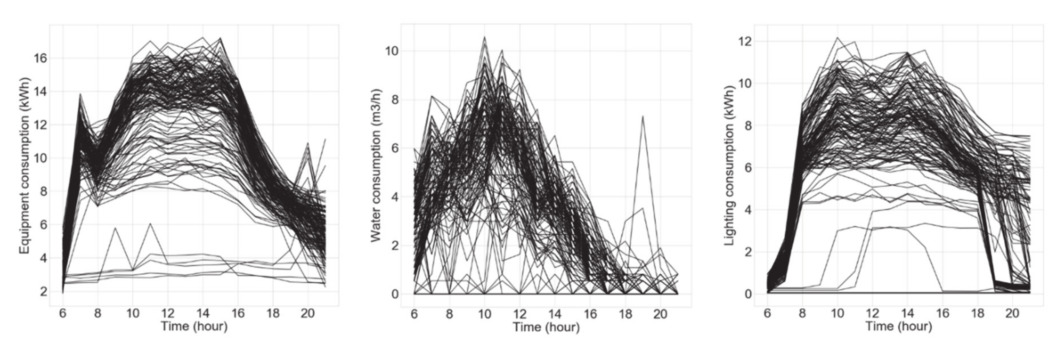
The unsupervised clustering method k-means was used on the same dataset as presented in Section 3.1. The dataset was split into day profiles so that the days could be clustered. The time between 06:00 and 21:00 was used for the profile, which made the day profile size of 16 values. In Figure 10, the three graphs presented contain day profiles with one of the variables, where lines represent the consumption of every weekday in the dataset. The data in each graph serves as an input for the k-means algorithm. From these graphs, it can be seen that equipment electricity consumption has two parts, where some days had significantly lower consumption and the rest with higher. Furthermore, higher consumption days could be divided into additional two parts: the lower part with fewer days (less dense part of the graph) and the higher part (dense part). It should be noted that it was more difficult to divide the graphs with lighting and especially with water consumption. The method used for selecting which variables (consumptions) could be used in the clustering algorithm and in how many (k) clusters should the dataset be divided, is discussed in the following section.
3.3.1. Choosing a Suitable Number of Clusters
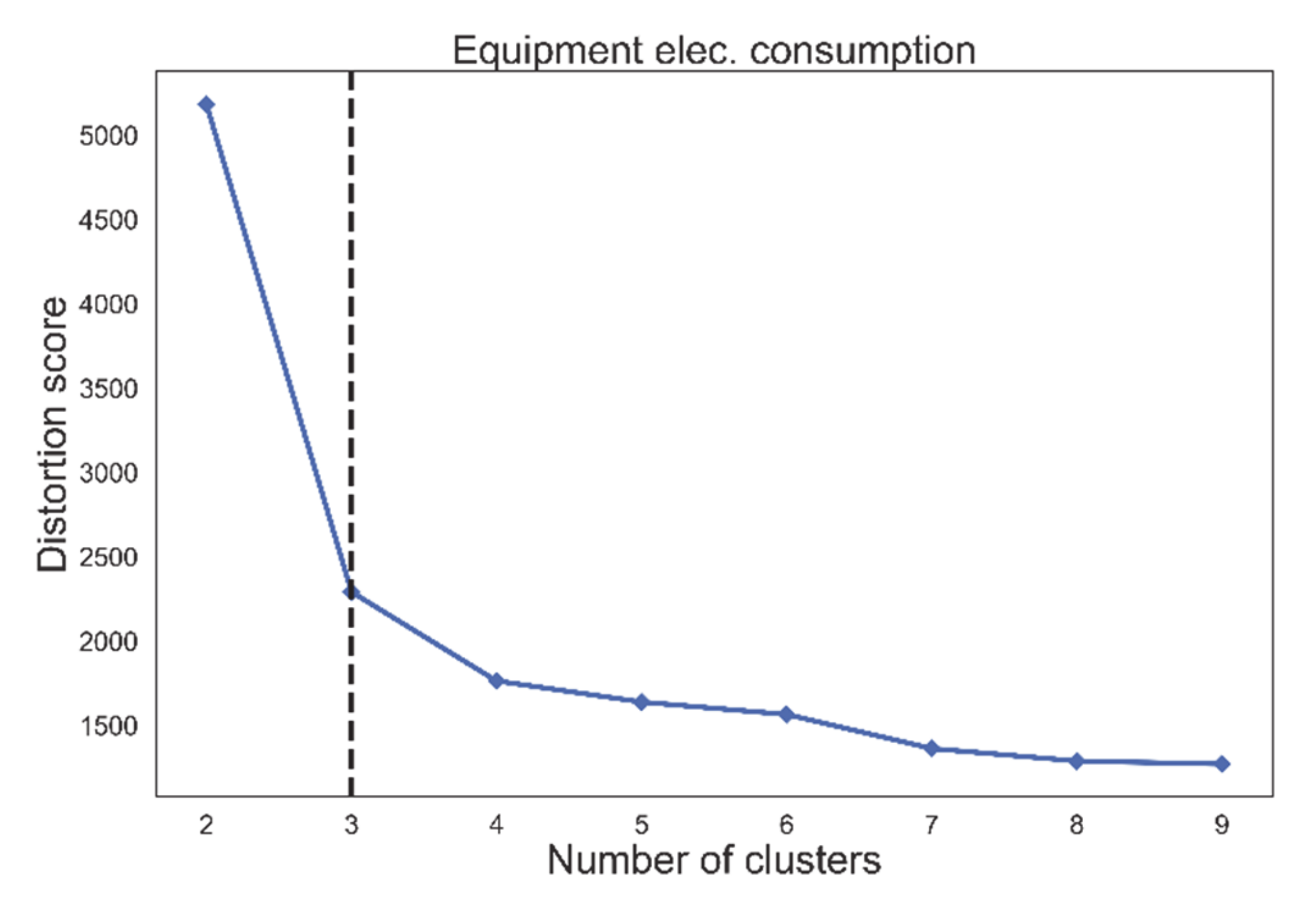
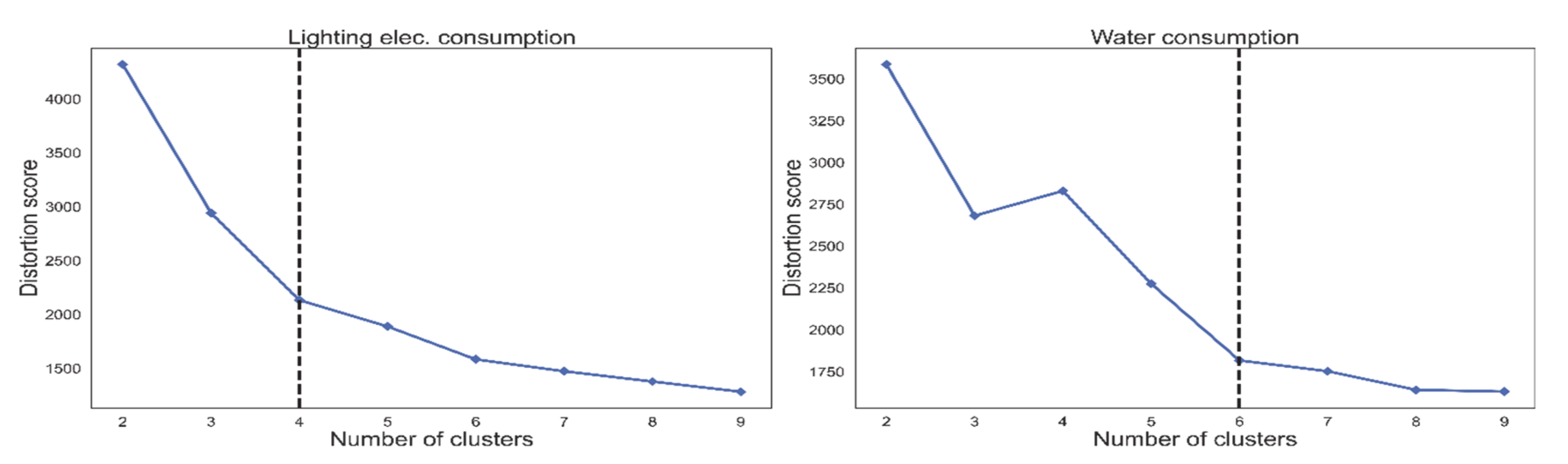
In Section 2.3, the method of choosing a suitable number of clusters, k, was explained. The Elbow method was applied by calculating k-means with the range of values for the k from two to nine. In Figure 11, the plotted line with distortion score for equipment electricity consumption over a different number of clusters, k, can be seen. The dotted line is showing the “elbow” of the curve which represents the selected value for k using the Elbow method. In the case of equipment consumption, the optimal number of clusters was three. A similar analysis was done for lighting electricity consumption and water consumption, which can be seen in Figure 12, where the optimal number of clusters was chosen to be four and six, respectively.
3.3.2. Clustering Results
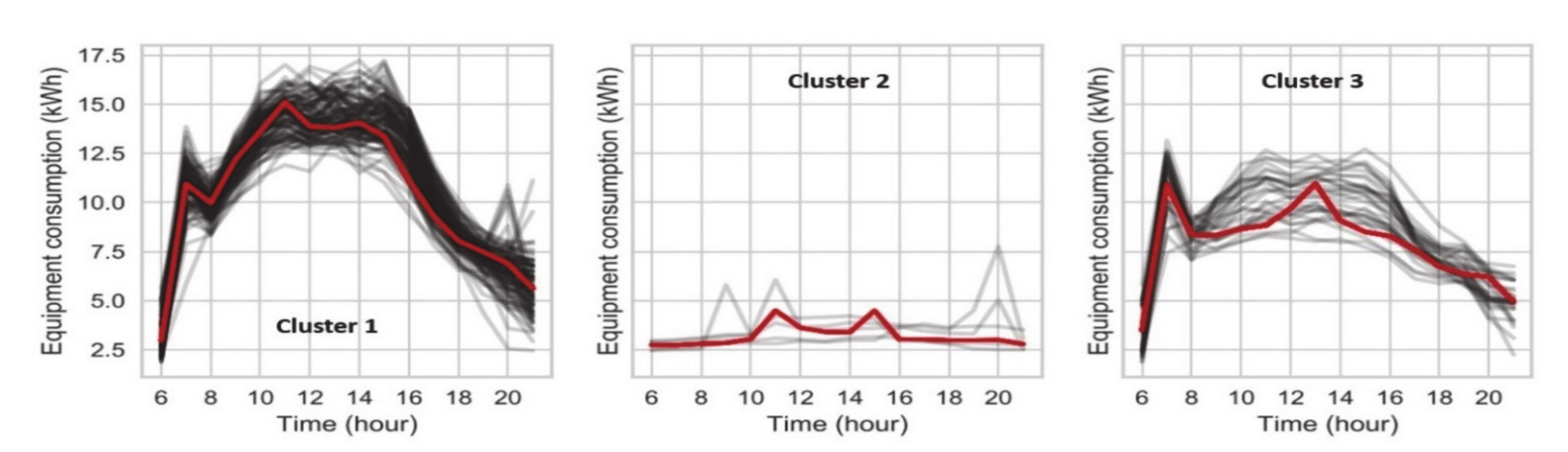
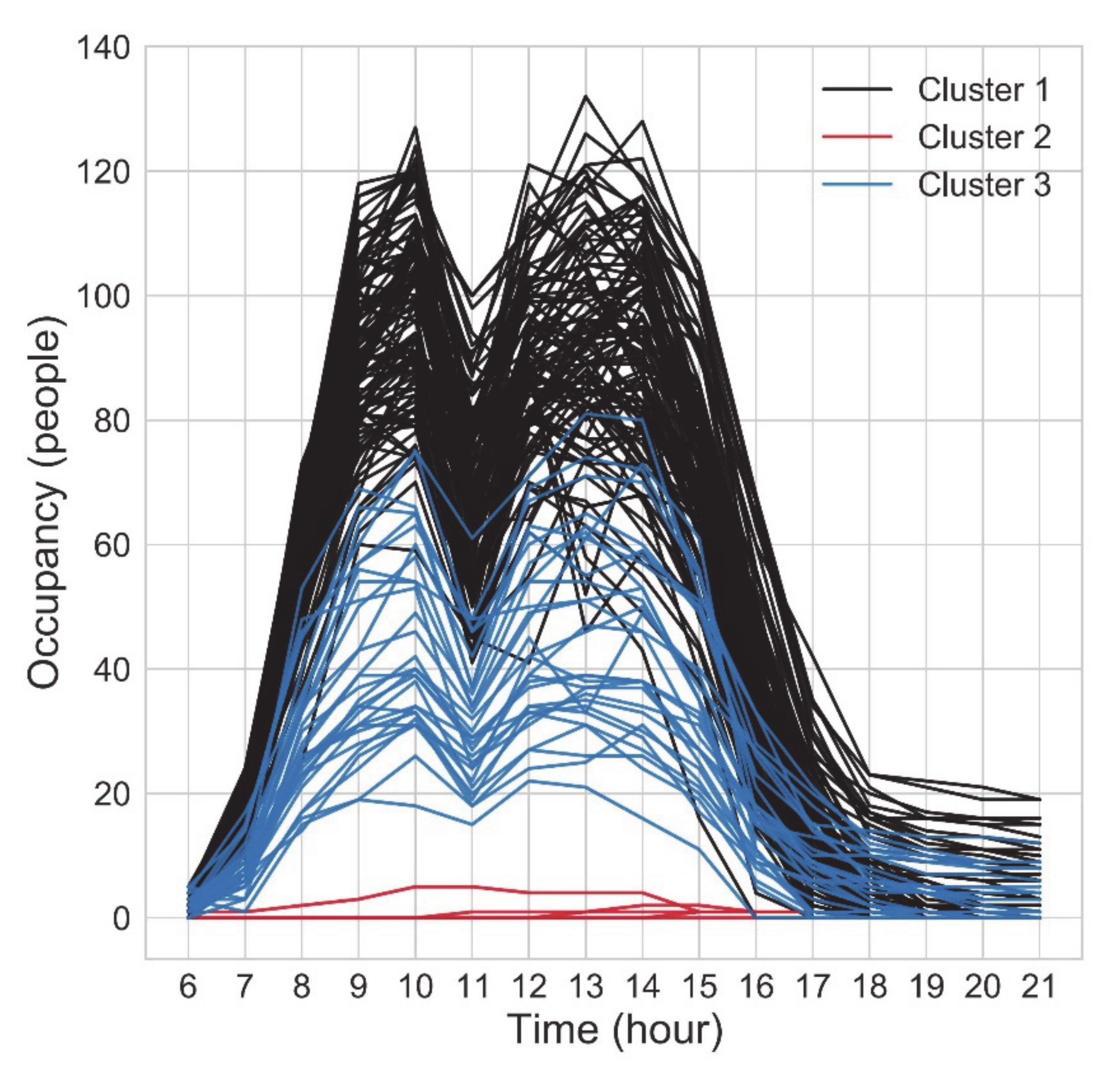
In Figure 13, three clusters of equipment electricity consumption are presented, together with day profiles of consumption belonging to each cluster (black lines) and with the cluster centre (red line). Each of these clusters represents a typical equipment electricity consumption pattern for the case floor. Since the office equipment consumption was mostly influenced by occupancy (e.g., computers), the assumption was that by clustering this consumption, the occupancy patterns could be found. In Figure 14, the occupancy measured by people counting cameras is presented with each day profile coloured by the belonging cluster. The highest occupancy belonged to the first cluster (black) and the days with the lowest occupancy to the second cluster (red), while the days with occupancy in between belonged to the third cluster (blue). This figure shows that there was a good correlation between measured equipment consumption and office occupancy. Correlation was most visible in the second cluster, where occupancy was nearly zero and consumption was low, compared to the other days. The first and third clusters were not clearly divided since they contained some border cases, which meant that certain days could potentially belong to either of those clusters. This was not the case with the second cluster, where belonging days with their consumption (and occupancy) had a clear membership.
Another way to analyse was when people had their summer vacation. Furthermore, in the same cluster, there were “bridge” days or days between the public holiday and a weekend, which some people took as a day off. These, a total of 29 days, were for the sake of simplicity called “semi-holidays” in this study. The largest group of the results was by looking at the date of the days in each cluster. In Cluster 2, all belonging days were public holidays in Finland, such as Labour Day (1st of May), Easter Friday and Monday, Ascension Day and Midsummer Day. The days in Cluster 3, with its medium level of consumption and occupancy were days when many days were regular working days which were clustered to Cluster 1, with a total of 107 days. Based on this analysis, it could be said that Cluster 1 could be called a high occupancy level, Cluster 2 as a low occupancy level and Cluster 3 as a medium occupancy level.
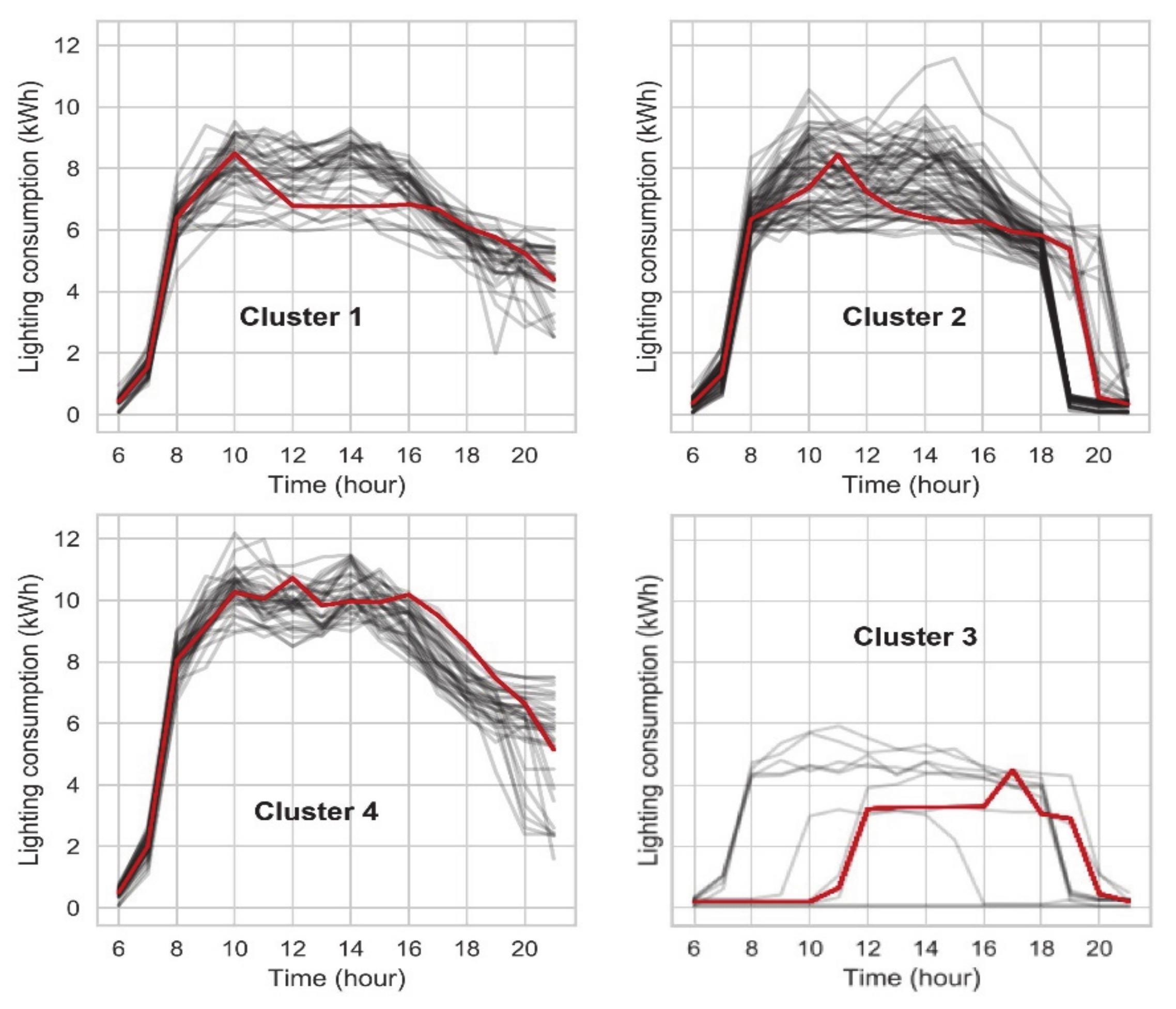
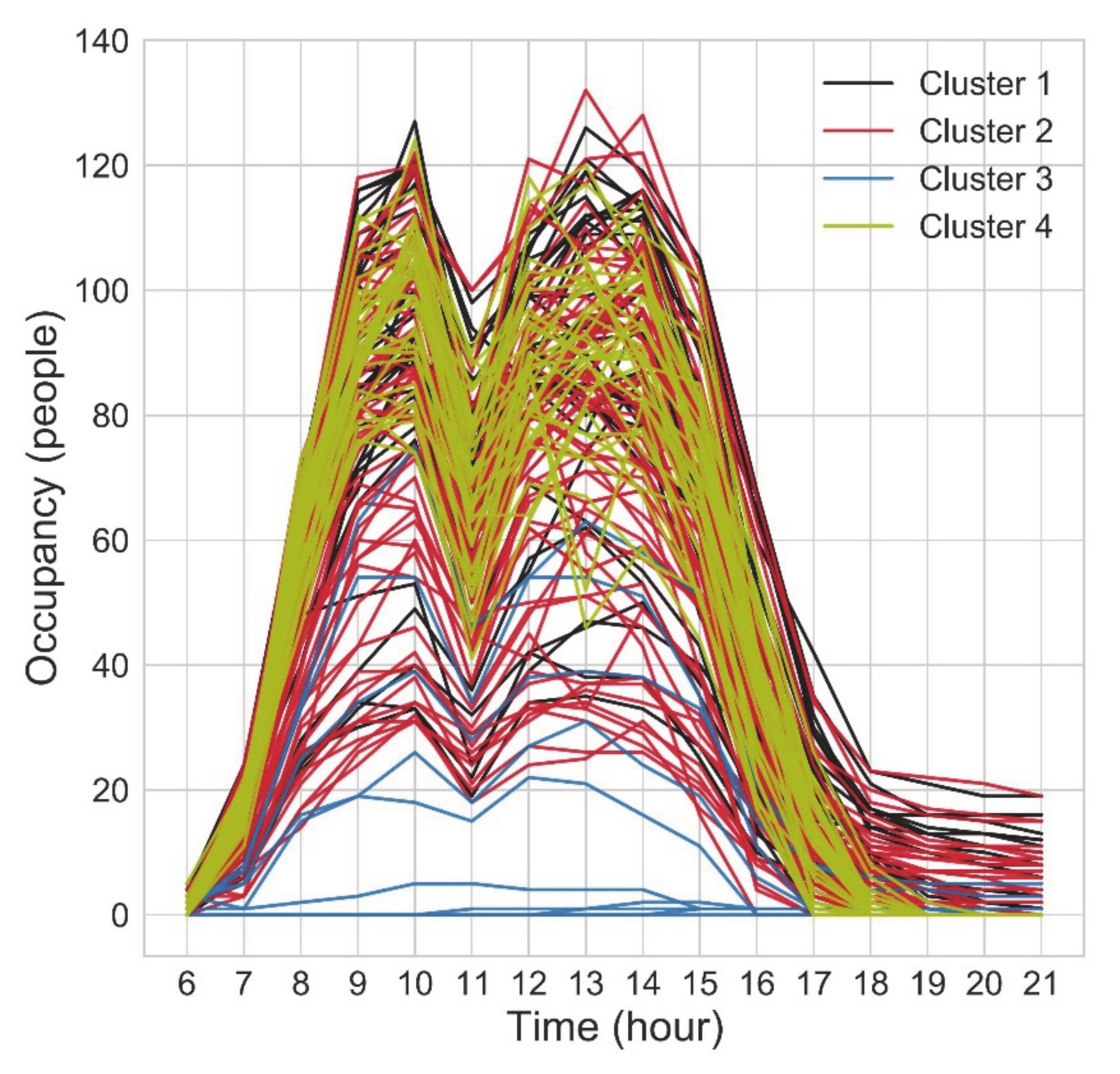
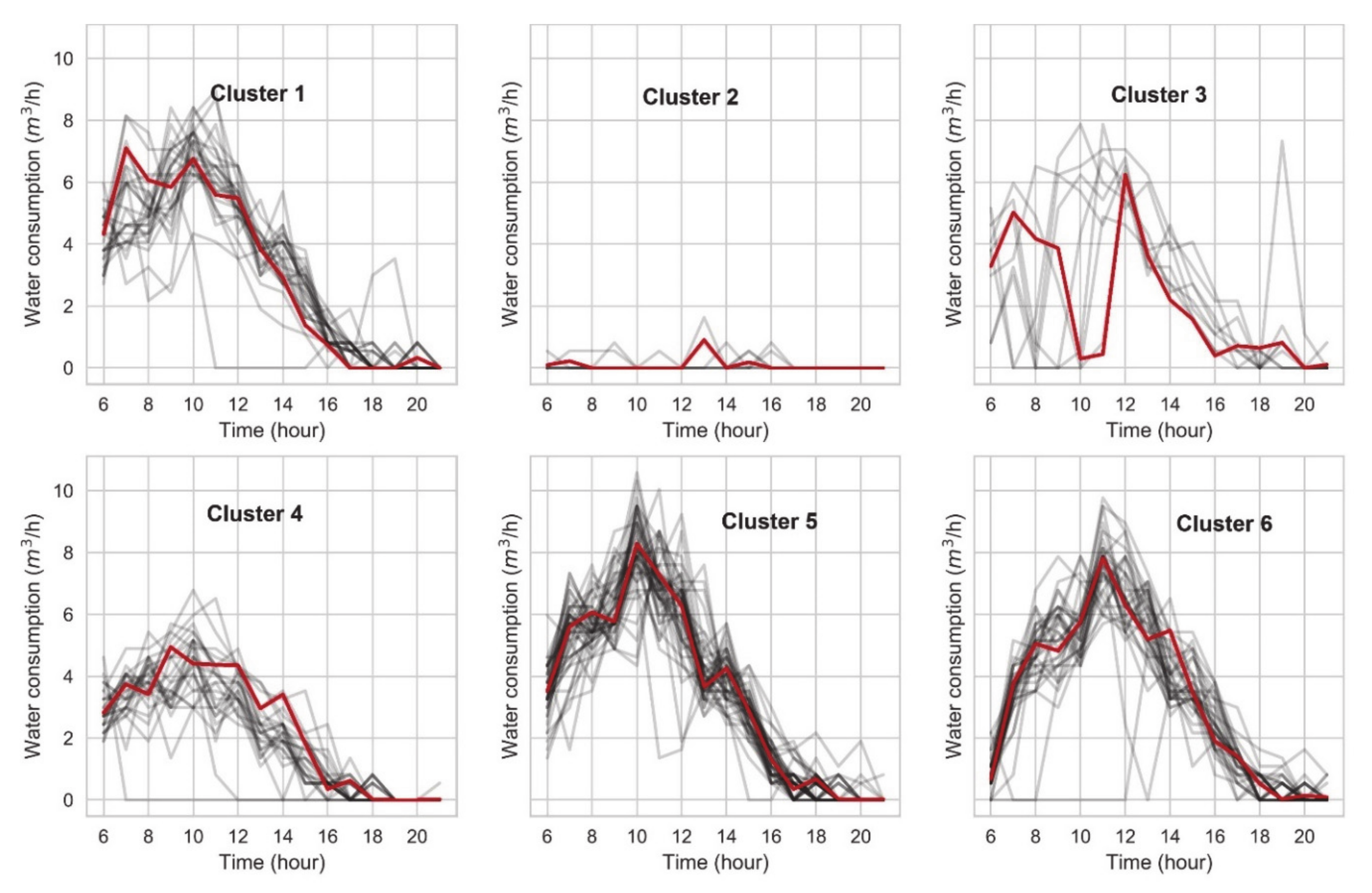
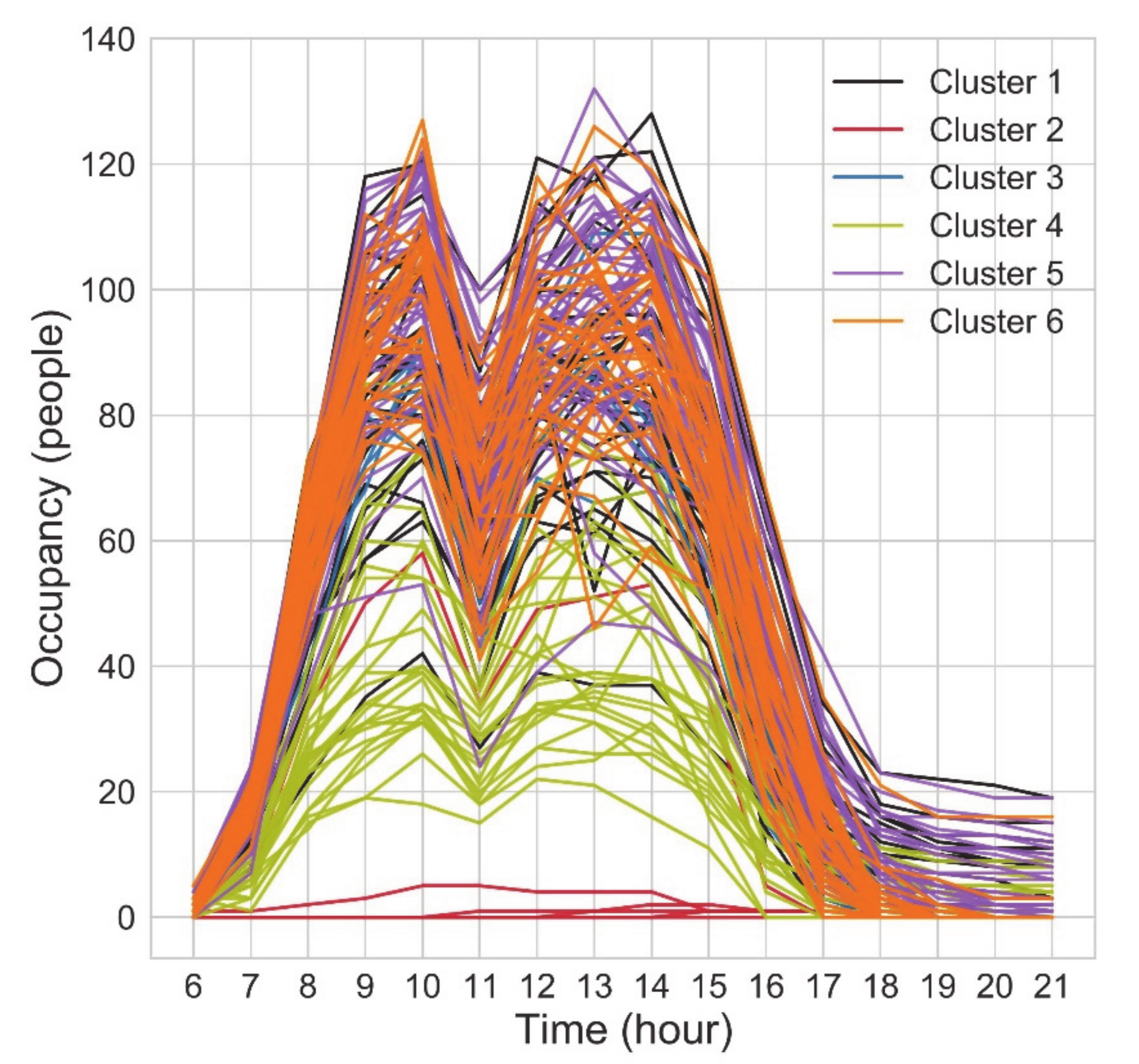
Following the equipment electricity consumption, the same method was performed on electricity consumption for office lighting and water consumption. Based on the findings from the Elbow method from Section 3.3.1, lighting consumption was clustered into four clusters, while water into six. Four clusters of lighting consumption are presented in Figure 15. In Cluster 3, days with zero and medium consumption were clustered together. In Figure 16, occupancy day profiles are coloured into four colours to represent the four clusters of lighting consumption. The lines representing lighting consumption day profiles were interlaced between different clusters, which meant that clustering the lighting consumption did not group the occupancy days into a logical order. The same conclusion can be seen from six clusters of water consumption (Figure 17 and Figure 18).
3.3.3. Summary of the Unsupervised Method Results
With the unsupervised method, this study was able to cluster the days by the level of the office occupancy using sub-metered office equipment electricity consumption. In the case study office, the three levels of occupancy were found:
- Zero (or nearly zero) occupancy level, occurring during the holidays,
- Medium occupancy level, occurring mostly during the “semi-holidays” (vacation and holiday bridge days),
- High occupancy level, occurring during regular working days.
Clustering the lighting electricity consumption or water consumption was not successful in finding the occupancy level of the office.
4. Discussion
This study and its results have tried to make several contributions. First, was to find information on building occupancy, which is usually not available, by using the data which is more common in buildings. Secondly, to increase the value of energy and water consumption sub-metering in commercial buildings. Last, is to promote the smart building concept where one data stream can be used for multiple purposes. Further research is needed to reinforce these contributions, especially regarding scaling the methods to real-world applications.
Foremost is to mention the limitations of this study, which are concerning the data collection of ground truth and water consumption. Ground truth was collected with people counting software, which reported that more people arrive at the office than leave it. This limitation is concerning the supervised method while giving another motive for the exploration of unsupervised methods. Despite this limitation, other possible methods for continuous long-term occupancy were not possible in our case study and are probably of even lower accuracy. Furthermore, the goal of this study was not the development of the method of high accuracy, but a method that will give more insight than usually available. Regarding water consumption, the issue is that it is not sub-metered for the floor, which might decrease its correlation with measured occupancy. This limitation could be one of the reasons why water consumption showed lower results with the unsupervised method, while with the supervised method, it was combined with other predictors. Additionally, to note is that sub-metering of water consumption is very rare in Finland.
Two methods of data mining studied in this work have been successful in discovering information about the office occupancy from the sub-metering. With the supervised method, this study proved that it is possible to predict the number of occupants in a larger office facility by using metered equipment, lighting electricity consumption or using water consumption. Earlier studies have mostly worked on detecting the occupancy or the occupancy level on a smaller scale. On the other hand, to use the supervised method, a long-term continuous collection campaign of ground truth is necessary. One way to do it is by installing the cameras with people counting software above all entrances to the target building area for a long enough period (30 to 90 days by the results of this work). In our experience, the biggest challenge was the installation permission of cameras, since that brings privacy and security issues. Permission was needed from the building owner, tenant and the IT department. Scaling this solution to a broader group of buildings could be problematic if the privacy issue is not possible to solve. Therefore, other methods, e.g., unsupervised methods, are appreciated where ground truth data is not required.
The unsupervised method developed in this work was able to cluster the days by the level of the office occupancy using equipment electricity consumption. In the case study office, the three levels of occupancy were found: zero (low), medium and high. Regular working days belonged mostly to the high occupancy level and were not divided into more than one level. A reason for this could be that even though individuals can work remotely, the overall office occupancy pattern does not have clear dividable groups. The medium level contains mostly days that have occupancy between a normal working day and a public holiday. These days are usually between holidays and weekends or during vacation periods. Although it is important to note that medium and high occupancy levels do not have a clear boundary, which means that some of the days could belong to either of the clusters.
The way of working could change radically in the future and remote work will become more common. This means that there could be fewer regular working days and more irregular days. Having insight into which days and how many in a year are irregular can help to better manage buildings from the technical and the real-estate perspective.
Methods proposed in this study could help with the EU’s goal of developing a sustainable energy system by increasing the ability of building systems to adapt to their occupancy. The prediction of occupancy number and level could be used as an input to the building performance simulations. Comparing the overall building energy consumption with predicted occupancy could enable tracking the energy consumed per person, which could be used for optimising HVAC system operation. Occupancy information is vital for the demand response in buildings, where knowing the occupancy patterns can help with predicting the energy need and further optimise the performance with a smart energy system.
Furthermore, the real-estate field can benefit greatly by having continuous insight into building occupancy, which can be used for office space management. Managing office space and its usage is becoming more critical because of the rise in popularity of remote work and high real-estate costs. Remote work has been growing for a while, and recently during the COVID-19 pandemic, it has become the new norm. Its popularity is expected to continue even after the end of the pandemic. Employees will want to continue enjoying the convenience of remote work; at the same time, the fear of potential new virus outbreaks could demand a need for a reasonable distance of workers in the office. Consequently, office space will have a lower occupancy rate, which could make them a target of cost-saving measures for companies, because of the resulting economic recession after the pandemics.
Scope for future work is to assess the scalability of the proposed methods, on an area with a different size than the case study floor and in other buildings. Especially the unsupervised method, since it does not require continuous ground truth data collection, which makes it easier for commercial applications. Although, lighter methods for verifying an unsupervised method should be studied, which could include even manual building walkthroughs. Enriching the proposed unsupervised method by using multiple predictors or even including other widely available signals in building such as Wi-Fi, should be investigated. The unsupervised method should be tested in smaller areas, such as different floor wings, or office departments, which could increase the granularity and the value of insight. Furthermore, the novel concept in machine learning called transfer learning should be investigated. With the transfer learning concept, a supervised model trained on one building could be transferred to a similar building and therefore reduce the need for a good ground truth dataset for every building.
5. Conclusions
The current study aimed to examine the possibility of utilising sub-metered electricity and water consumption with data mining methods to determine the occupancy of the office. Two approaches were tested: supervised and unsupervised data mining methods. The supervised method was done using a Random Forest algorithm, while the unsupervised method used the clustering k-means algorithm.
The results of this study have shown that it is possible to predict the number of people on a larger office floor with the explained variance at 96% using sub-metered electricity and water consumption with the supervised method. Best results came with using all available predictors, followed by electricity consumption used for lighting and sockets and then by water consumption. The lowest-performing result was by using lighting electricity as the main predictor, but still it had a decent explained variance of 93%. Furthermore, with the help of data sufficiency and generalisation analysis, the performance of the method was tested during different periods and with different training lengths. This analysis showed that performance is at a similar level as with the main testing period during the regular working weeks, while the lower performance of the model was for irregular weeks, such as during vacations. The analysis has also shown that the minimum recommended length of the training dataset should be between one and three months. Since the continuous collection of occupancy ground truth in a building, has its earlier mentioned problems, this study has also explored the way of using the unsupervised method with consumption data to find insight into the office occupancy.
With the unsupervised method, it was possible to cluster the days into three occupancy levels: high, medium and low without the need for ground truth. This clustering was possible by using the sub-metered office equipment (from sockets) electricity consumption. The ground truth was used only for the verification of the method. On the other hand, using the same method with the lighting electricity consumption and the water consumption did not give satisfactory results when comparing their clusters to the ground truth.
Author Contributions
Conceptualization: D.S. Methodology: D.S. Formal analysis: D.S. Investigation: D.S. Data curation: D.S. Writing—original draft preparation: D.S. Writing—review and editing: R.K., J.J. Supervision: R.K., J.J. All authors have read and agreed to the published version of the manuscript.
Funding
This research was funded by Business Finland through the project Smart Otaniemi.
Acknowledgments
The authors would like to thank Aalto University and Granlund Oy for making this research possible.
Conflicts of Interest
The authors declare no conflict of interest.
Nomenclature
| DBA | DTW barycenter averaging |
| DTW | Dynamic time warping |
| EV | Explained variation |
| FD | First order difference |
| FDE | First order difference—equipment |
| FDL | First order difference—lighting |
| FDT | First order difference—total |
| FDW | First order difference—water |
| k | Number of clusters |
| MA1 | 1-step Moving average |
| MA1E | 1-step Moving average—equipment |
| MA1L | 1-step Moving average—lighting |
| MA1T | 1-step Moving average—total |
| MA1W | 1-step Moving average—water |
| MA2 | 2-step Moving average |
| MA2E | 2-step Moving average—equipment |
| MA2L | 2-step Moving average—lighting |
| MA2T | 2-step Moving average—total |
| MA2W | 2-step Moving average—water |
| MBE | Mean bias error |
| RMSE | Root mean square error |
| SD | Second order difference |
| SDE | Second order difference—equipment |
| SDL | Second order difference—lighting |
| SDT | Second order difference—total |
| SDW | Second order difference—water |
References
- EUR-Lex. European Union Directive 2018/844 of the European Parliament and of the Council of 30 May 2018 amending Directive 2010/31/EU on the energy performance of buildings and Directive 2012/27/EU on energy efficiency. Off. J. Eur. Union 2018, 156, 75–91. [Google Scholar]
- UN Environment; International Energy Agency. Towards a Zero-Emission, Efficient, and Resilient Buildings and Construction Sector; Global Status Report; United Nations: New York, NY, USA, 2017. [Google Scholar]
- Yu, Z.; Fung, B.C.M.; Haghighat, F. Extracting knowledge from building-related data—A data mining framework. Build. Simul. 2013, 6, 207–222. [Google Scholar] [CrossRef]
- International Energy Agency. Definition and Simulation of Occupant Behavior in Buildings International Energy Agency, EBC Annex 66 Definition and Simulation of Occupant Behavior in Buildings; The Regents of the University of California and Tsinghua University, China; International Energy Agency: Paris, France, 2018; ISBN 9780999696477. [Google Scholar]
- Yan, D.; Hong, T.; Dong, B.; Mahdavi, A.; Oca, S.D.; Gaetani, I.; Feng, X. IEA EBC Annex 66: Definition and simulation of occupant behavior in buildings. Energy Build. 2017, 156, 258–270. [Google Scholar] [CrossRef] [Green Version]
- Cuerda, E.; Guerra-Santin, O.; Sendra, J.J.; Neila González, F.J. Comparing the impact of presence patterns on energy demand in residential buildings using measured data and simulation models. Build. Simul. 2019, 12, 985–998. [Google Scholar] [CrossRef]
- Zhao, J.; Lasternas, B.; Lam, K.P.; Yun, R.; Loftness, V. Occupant behavior and schedule modeling for building energy simulation through office appliance power consumption data mining. Energy Build. 2014, 82, 341–355. [Google Scholar] [CrossRef]
- Ahn, K.; Kim, D.; Park, C.; Wilde, P. De Predictability of occupant presence and performance gap in building energy simulation. Appl. Energy 2017, 208, 1639–1652. [Google Scholar] [CrossRef]
- Tianzhen, H.; Langevin, J.; Sun, K. Building simulation: Ten challenges. Build. Simul. 2018, 871–898. [Google Scholar] [CrossRef] [Green Version]
- Zaki, M.J.; Meira, W.J. Data Mining and Analysis; Cambridge University Press: Cambridge, UK, 2014; ISBN 9780521766333. [Google Scholar]
- Fan, C.; Xiao, F.; Li, Z.; Wang, J. Unsupervised data analytics in mining big building operational data for energy efficiency enhancement: A review. Energy Build. 2018, 159, 296–308. [Google Scholar] [CrossRef]
- Kleiminger, W.; Beckel, C.; Staake, T.; Santini, S. Occupancy Detection from Electricity Consumption Data. In Proceedings of the 5th ACM Workshop on Embedded Systems For Energy-Efficient Buildings, Rome, Italy, 14–15 November 2013; pp. 1–8. [Google Scholar] [CrossRef] [Green Version]
- Mora, D.; Fajilla, G.; Austin, M.C.; De Simone, M. Occupancy patterns obtained by heuristic approaches: Cluster analysis and logical flowcharts. A case study in a university office. Energy Build. 2019, 186, 147–168. [Google Scholar] [CrossRef]
- Yang, L.; Ting, K.; Srivastava, M.B. Inferring occupancy from opportunistically available sensor data. In Proceedings of the 2014 IEEE International Conference on Pervasive Computing and Communications (PerCom), Budapest, Hungary, 24–28 March 2014; pp. 60–68. [Google Scholar] [CrossRef]
- Kleiminger, W.; Beckel, C.; Santini, S. Household occupancy monitoring using electricity meters. In Proceedings of the 2015 ACM International Joint Conference on Pervasive and Ubiquitous Computing, Osaka, Japan, 7–11 September 2015; pp. 975–986. [Google Scholar] [CrossRef] [Green Version]
- Akbar, A.; Nati, M.; Carrez, F.; Moessner, K. Contextual occupancy detection for smart office by pattern recognition of electricity consumption data. In Proceedings of the 2015 IEEE International Conference on Communications (ICC), London, UK, 8–12 June 2015; pp. 561–566. [Google Scholar] [CrossRef]
- Razavi, R.; Gharipour, A.; Fleury, M.; Justice, I. Energy & Buildings Occupancy detection of residential buildings using smart meter data: A large-scale study. Energy Build. 2019, 183, 195–208. [Google Scholar] [CrossRef]
- Rhodes, J.D.; Cole, W.J.; Upshaw, C.R.; Edgar, T.F.; Webber, M.E. Clustering analysis of residential electricity demand profiles. Appl. Energy 2014, 135, 461–471. [Google Scholar] [CrossRef] [Green Version]
- McLoughlin, F.; Duffy, A.; Conlon, M. A clustering approach to domestic electricity load profile characterisation using smart metering data. Appl. Energy 2015, 141, 190–199. [Google Scholar] [CrossRef] [Green Version]
- Pan, S.; Wang, X.; Wei, Y.; Zhang, X.; Gal, C.; Ren, G.; Yan, D.; Shi, Y.; Wu, J.; Xia, L.; et al. Cluster analysis for occupant-behavior based electricity load patterns in buildings: A case study in Shanghai residences. Build. Simul. 2017, 10, 889–898. [Google Scholar] [CrossRef]
- Yang, J.; Ning, C.; Deb, C.; Zhang, F.; Cheong, D.; Lee, S.E.; Sekhar, C.; Tham, K.W. K-Shape clustering algorithm for building energy usage patterns analysis and forecasting model accuracy improvement. Energy Build. 2017, 146, 27–37. [Google Scholar] [CrossRef]
- D’Oca, S.; Hong, T. Occupancy schedules learning process through a data mining framework. Energy Build. 2015, 88, 395–408. [Google Scholar] [CrossRef] [Green Version]
- Liang, X.; Hong, T.; Qiping, G. Occupancy data analytics and prediction: A case study. Build. Environ. 2016, 102, 179–192. [Google Scholar] [CrossRef] [Green Version]
- Causone, F.; Carlucci, S.; Ferrando, M.; Marchenko, A.; Erba, S. A data-driven procedure to model occupancy and occupant-related electric load profiles in residential buildings for energy simulation. Energy Build. 2019, 202, 109342. [Google Scholar] [CrossRef]
- Dong, B.; Kjærgaard, M.B.; De Simone, M.; Gunay, H.B.; O’Brien, W.; Mora, D.; Dziedzic, J.; Zhao, J. Sensing and data acquisition. In Exploring Occupant Behavior in Buildings: Methods and Challenges; Springer: Cham, Switzerland, 2017; pp. 77–105. ISBN 9783319614649. [Google Scholar]
- Dong, B.; Yan, D.; Li, Z.; Jin, Y.; Feng, X.; Fontenot, H. Modeling occupancy and behavior for better building design and operation—A critical review. Build. Simul. 2018, 11, 899–921. [Google Scholar] [CrossRef]
- Kuutti, J.; Blomqvist, K.H.; Sepponen, R.E. Performance of Commercial Over-Head Camera Sensors in Recognizing Patterns of Two and Three Persons: A Case Study. In Proceedings of the 2013 IEEE Jordan Conference on Applied Electrical Engineering and Computing Technologies (AEECT), Amman, Jordan, 3–5 December 2013. [Google Scholar]
- Liaw, A.; Wiener, M. Classification and Regression by randomForest. R News 2002, 3, 18–22. [Google Scholar]
- Pedregosa, F.; Varoquaux, G.; Gramfort, A.; Michel, V.; Thirion, B.; Grisel, O.; Blondel, M.; Prettenhofer, P.; Weiss, R.; Dubourg, V.; et al. Scikit-learn: Machine Learning in Python. J. Mach. Learn. Res. 2011, 12, 2825–2830. [Google Scholar]
- Liao, T.W. Clustering of time series data—A survey. Pattern Recognit. 2005, 38, 1857–1874. [Google Scholar] [CrossRef]
- Sakoe, H.; Chiba, S. Dynamic programming algorithm optimization for spoken word recognition. IEEE Trans. Acoust. 1978, 26, 43–49. [Google Scholar] [CrossRef] [Green Version]
- Petitjean, F.; Ketterlin, A.; Gançarski, P. A global averaging method for dynamic time warping, with applications to clustering. Pattern Recognit. 2011, 44, 678–693. [Google Scholar] [CrossRef]
- Tavenard, R.; Faouzi, J.; Vandewiele, G.; Divo, F.; Androz, G.; Holtz, C.; Payne, M.; Yurchak, R.; Rußwurm, M.; Kolar, K.; et al. Tslearn: A Machine Learning Toolkit Dedicated to Time-Series Data. 2017. Available online: https://tslearn.readthedocs.io/ (accessed on 23 March 2020).
- Thorndike, R.L. Who belongs in the family. Psychometrika 1953, 18, 267–276. [Google Scholar] [CrossRef]
- Satopää, V.; Albrecht, J.; Irwin, D.; Raghavan, B. Finding a “ Kneedle ” in a Haystack: Detecting Knee Points in System Behavior. In Proceedings of the 31st International Conference on Distributed Computing Systems Workshops, IEEE, Minneapolis, MN, USA, 20–24 June 2011; pp. 1–6. [Google Scholar]
- Bengfort, B.; Bilbro, R.; Danielsen, N.; Gray, L.; McIntyre, K.; Roman, P.; Morris, A.; Sharma, S.; Chestnut, M.; Garod, M.; et al. Yellowbrick 2018. Available online: https://www.scikit-yb.org/ (accessed on 23 March 2020).
- Granlund Granlund Manager. Available online: https://www.granlundmanager.com/ (accessed on 23 March 2020).
- Cerqueira, V.; Torgo, L.; Mozetic, I. Evaluating time series forecasting models: An empirical study on performance estimation methods. Mach. Learn. 2020, 109, 1997–2028. [Google Scholar] [CrossRef]
Figure 1.
The pilot floor of this study consists of open layout offices and meeting rooms.

Figure 2.
Scheme of supervised data mining method for predicting the number of occupants.

Figure 3.
Scheme of unsupervised data mining method for predicting the office occupancy level.

Figure 4.
Pearson’s correlation matrix between lighting, equipment and water consumption and occupancy ground truth.
Figure 4.
Pearson’s correlation matrix between lighting, equipment and water consumption and occupancy ground truth.

Figure 5.
Measured and predicted occupancy during the test period. The predicted occupancy was calculated using all predictors.
Figure 5.
Measured and predicted occupancy during the test period. The predicted occupancy was calculated using all predictors.

Figure 6.
Comparison between predicted occupancy of different predictors and with the measured occupancy for a selected day.
Figure 6.
Comparison between predicted occupancy of different predictors and with the measured occupancy for a selected day.

Figure 7.
Comparison between models with different predictors by hourly RMSE for an average day of the test period.
Figure 7.
Comparison between models with different predictors by hourly RMSE for an average day of the test period.

Figure 8.
Occupancy prediction error (EV) for different testing periods as a function of training duration.
Figure 8.
Occupancy prediction error (EV) for different testing periods as a function of training duration.

Figure 9.
Occupancy prediction error (RMSE) for different testing periods as a function of training duration.
Figure 9.
Occupancy prediction error (RMSE) for different testing periods as a function of training duration.

Figure 10.
Day energy consumption profiles of each studied variable of the unsupervised method, where each line represents the consumption for one day in the dataset. Equipment consumption (left), water consumption (centre) and lighting consumption (right).
Figure 10.
Day energy consumption profiles of each studied variable of the unsupervised method, where each line represents the consumption for one day in the dataset. Equipment consumption (left), water consumption (centre) and lighting consumption (right).

Figure 11.
Distortion score with a different number of clusters (k) for equipment electricity consumption. Using the elbow method the optimal number of clusters is selected to be three (dotted line).
Figure 11.
Distortion score with a different number of clusters (k) for equipment electricity consumption. Using the elbow method the optimal number of clusters is selected to be three (dotted line).

Figure 12.
Distortion score with a different number of clusters (k) for lighting electricity consumption (left) and water consumption (right). The optimal value for k is four and six, respectively.
Figure 12.
Distortion score with a different number of clusters (k) for lighting electricity consumption (left) and water consumption (right). The optimal value for k is four and six, respectively.

Figure 13.
Equipment electricity consumption clusters. (Black) lines represent the day profiles of consumption, while (red) lines represent the cluster centre.
Figure 13.
Equipment electricity consumption clusters. (Black) lines represent the day profiles of consumption, while (red) lines represent the cluster centre.

Figure 14.
Occupancy day profiles coloured by clusters of equipment electricity consumption.

Figure 15.
Lighting electricity consumption clusters. (Black) lines represent the day profiles of consumption, while (red) lines represent the cluster (centre).
Figure 15.
Lighting electricity consumption clusters. (Black) lines represent the day profiles of consumption, while (red) lines represent the cluster (centre).

Figure 16.
Occupancy day profiles coloured by clusters of lighting electricity consumption.

Figure 17.
Water consumption clusters. (Black) lines represent the day profiles of consumption, while (red) lines represent the cluster (centre).
Figure 17.
Water consumption clusters. (Black) lines represent the day profiles of consumption, while (red) lines represent the cluster (centre).

Figure 18.
Occupancy day profiles coloured by clusters of water consumption.


Table 1.
List of features used in this study and their equation.
| # | Feature | Description |
|---|---|---|
| 1 | First-order difference (FD) | |
| 2 | Second-order difference (SD) | |
| 3 | 1-step Moving average (MA1) | |
| 4 | 2-step Moving average (MA2) |
Table 2.
Selected combinations of the features that were used together with the main predictor.
| Main Predictor | Selected Features |
|---|---|
| Lighting | FDL, month, hour, weekday |
| Equipment | FDE, MA2E, hour, weekday |
| Light and Equipment (separate) | SDL, SDE, MA2L, MA2E, hour, weekday |
| Total floor electric consumption (Light and Equipment summed) | FDT, SDT, month, hour, weekday |
| Water consumption | FDW, MA1W, MA2W, hour, weekday |
| All predictors | FDL, SDL, FDE, SDE, SDW, MA1E, MA1W, month, hour, weekday |
Table 3.
Results of the supervised method for occupancy rate prediction shown through three error indices: RMSE, MBE and explained variation (EV).
Table 3.
Results of the supervised method for occupancy rate prediction shown through three error indices: RMSE, MBE and explained variation (EV).
| Set of Predictors | RMSE (Persons) | MBE (Persons) | EV (%) |
|---|---|---|---|
| Lighting | 10.52 | −1.6 | 93 |
| Equipment | 8.87 | −2.34 | 95 |
| Light and Equipment | 8.14 | −2.07 | 96 |
| Total floor electricity consumption | 8.8 | 0.41 | 95 |
| Water consumption | 9.67 | −0.5 | 94 |
| All predictors | 7.88 | −0.66 | 96 |
Publisher’s Note: MDPI stays neutral with regard to jurisdictional claims in published maps and institutional affiliations. |
© 2020 by the authors. Licensee MDPI, Basel, Switzerland. This article is an open access article distributed under the terms and conditions of the Creative Commons Attribution (CC BY) license (http://creativecommons.org/licenses/by/4.0/).
Share and Cite
MDPI and ACS Style
Stjelja, D.; Jokisalo, J.; Kosonen, R. From Electricity and Water Consumption Data to Information on Office Occupancy: A Supervised and Unsupervised Data Mining Approach. Appl. Sci. 2020, 10, 9089. https://doi.org/10.3390/app10249089
AMA Style
Stjelja D, Jokisalo J, Kosonen R. From Electricity and Water Consumption Data to Information on Office Occupancy: A Supervised and Unsupervised Data Mining Approach. Applied Sciences. 2020; 10(24):9089. https://doi.org/10.3390/app10249089
Chicago/Turabian StyleStjelja, Davor, Juha Jokisalo, and Risto Kosonen. 2020. "From Electricity and Water Consumption Data to Information on Office Occupancy: A Supervised and Unsupervised Data Mining Approach" Applied Sciences 10, no. 24: 9089. https://doi.org/10.3390/app10249089
Note that from the first issue of 2016, this journal uses article numbers instead of page numbers. See further details here.