Robust Resonant Controllers for Distributed Energy Resources in Microgrids
by
 , ,
, ,
Allal El Moubarek Bouzid
1 ,
,
Mohamed Zerrougui
2,
Seifeddine Ben Elghali
2,
Karim Beddiar
3,* and
Mohamed Benbouzid
4,5,*
1
Laboratoire des Sciences du Numérique de Nantes (LS2N-UMR CNRS 6004), Ecole Centrale de Nantes, 44321 Nantes, France
2
Laboratory of Information and Systems (LIS-UMR CNRS 7020), Aix-Marseille University, 13007 Marseille, France
3
Laboratoire d’Innovation Numérique pour les Entreprises et les Apprentissages au service de la Compétitivité des Territoires, Centre des Études Supérieures Industrielles, 2 Avenue de Provence, 29200 Brest, France
4
Institut de Recherche Dupuy de Lôme (UMR CNRS 6027 IRDL), University of Brest, 29238 Brest, France
5
Engineering Logistics College, Shanghai Maritime University, Shanghai 201306, China
*
Authors to whom correspondence should be addressed.
Appl. Sci. 2020, 10(24), 8905; https://doi.org/10.3390/app10248905
Submission received: 6 November 2020
/
Revised: 4 December 2020
/
Accepted: 7 December 2020
/
Published: 14 December 2020
(This article belongs to the Special Issue Microgrids/Nanogrids Implementation, Planning, and Operation)
Abstract
:Motivated by the problem of different types and variations of load in micro-grids, this paper presents robust proportional-resonant controllers with a harmonics compensator based on the internal model principle. These controllers ensure robust tracking of sinusoidal reference signals in distributed energy resource systems subject to load variation with respect to sinusoidal disturbances. The distributed generation resource and the resonant controllers are described using the augmented state system approach, allowing the application of the state feedback technique. In order to minimize the tracking error and ensure robustness against perturbation, a set of linear matrix inequalities (LMIs) are addressed for the synthesizing of controller gains. Finally, results obtained in the simulation for resonant compensators with the distributed energy system are presented, in which the controller is applied to the CC-CA inverter.
1. Introduction
Distributed energy resource (DER) systems are extensively used in micro-grids for the connection of renewable energy sources and storage [1]. However, this system must be able to maintain in its output voltage the same characteristics of the voltage provided by the electrical network to which they are connected, i.e., constant frequency and voltage amplitude and sine waveform, even when the primary network presents any failure (distortion, or even cut in the blackout supply). In practice, it is sought that, in the event of a power outage, for example, the equipment connected to the DER output will continue to operate normally to feed the locally connected loads. A basic method to obtain the proposed results is to compare the DER output voltage with a sinusoidal reference signal of the same waveform than the expected signal of the primary electrical network in normal operation [2]. However, the tracking of the reference signal becomes complex due to the non-linearities induced by the association of the different types of loads and the LCL filter connected at the output of the inverter. For example, the wide majority of electronic devices require direct current sources, equipped with a rectifier stage with full diodes bridge, which represents a great source of harmonic distortions due to the current waveform, and consequently the voltage in the grid [3].
Due to the critical nature of the loads, DER performance is regulated by international (ANSI/IEEE, 1986; IEC, 2011) standards [4], imposing conditions for the system’s transient and steady state performance. During transient, standards require a small variation in the output voltage amplitude and a fast recovery time when a load is added or removed from the system. In steady state, the output voltage of a DER must be a sinusoidal signal with constant amplitude and frequency. To be considered as a sinusoidal signal when subjected to periodic disturbances caused by non-linear loads, the output voltage THD (Total Harmonic Distortion) and IHD (Individual Harmonic) must be within limits defined in these standards. A fundamental performance requirement of a distributed energy resources (DER) system with sinusoidal output is to provide a voltage with low harmonic distortion, which operates even under uncertainties, parametric variations and non-linearities induced by phenomena such as delay and saturation and disturbances, which are very common in practice. This objective can be fulfilled by choosing an adequate control law.
Recently, considerable literature has been produced around the theme of DER control in microgrids to solve the above-cited problems. A major solution consists in the use of resonant compensators, adjusted to act on the fundamental frequency of the output and most significant harmonics. This method is based on the addition of harmonic modes (sine or cosine functions) in the direct control loop. The ideal resonant controller presents infinite gain at the resonance frequency, which allows us to reject the other components. The use of a set of resonant controllers in parallel allows the rejection of disturbances and reference tracking at selected frequencies. However, a high number of resonant compensators makes control tuning more complicated. Furthermore, it is necessary to take into account the ranges of the load and its variation in the problem formulation. Although there is a large number of published results dealing with DER system control, topics that still deserve further investigation are the proposition of controller design methodologies according to specific standards and the use of conditions based on Lyapunov functions for a more rigorous analysis of the stability and robust performance of the closed-loop system.
In the literature, different controllers have been applied to control the distributed energy system based on the inverter with an LC filter. In Reference [5], PID (Proportional Integral Derivative) controllers were proposed. However, these ones were based on the voltage RMS value to obtain the feedback signal. Thus, their use solves the problem of voltage amplitude, but, in general, it does not solve the problem of distortion of the output voltage waveform [6]. A cascaded voltage/current control based on a virtual impedance concept has been developed in [7]. This topology simultaneously improves the injected grid current and local load voltage in island and grid connected microgrids. An optimized proportional resonant (PR) controller taking account of the computational delay from the digital control system was proposed in [8]. A controller based on a polytopic model was proposed in [9] for the current controller development by taking into account the grid inductance variations and soft saturation. To minimize output current ripples and reduce the steady-state current deviation, a quasi proportional resonant controller was proposed in [10]. Generally, the proportional resonant controller parameters are tuned manually. However, in [8], the authors proposed an optimization tuning of the RCs controller. An adaptive PR controller was proposed in [11] to ensure a current tracking under grid parameter variations. The authors used a fourth order filter with the adaptive RC to estimate online the resonance frequency, and then the grid impedance variations. In order to reduce the steady state current error, a modified proportional resonant controller used for the inner current control loop and indirect vector controller at the rotating reference frame was proposed in [12]. A controller to compensate the resonance phenomena without knowing the system parameters and without affecting the controller bandwidth in island microgrids was proposed in [13]. A three degrees of freedom cascaded voltage/current controller based on theory was proposed in [14,15]. The main advantage of this controller is to ensure the stability of the closed-loop system and the robustness against parameter uncertainties.
To solve the above problems, the proposed method in this paper is based on the solution of optimization problems addressed by linear matrix inequalities (LMIs) formulation, which allows to concatenate the parameters of different resonant compensators acting in different frequencies. The proposed design method includes an easy solution to synthetizing the gains of the resonant controller, for a given capacity of the applied load range to distributed generation system units in the microgrid. The determination of gains is formalized through a convex optimization problem under a set of linear matrix inequalities constraints. In this paper, state feedback is used in conjunction with multiple resonant compensators that ensure the elimination of the steady state error and guarantee the rejection of multiple harmonics of the fundamental frequency produced by non-linear loads. In order to ensure the desired performances, the LMIs constraints construction is performed using a performance criterion throughout a robust regional poles placement [16,17].
Following this paper, a mathematical modeling of a DER system is proposed in Section 2. In Section 3 the proposed controller is presented, as well as the augmented model of the DER system and proportional resonant controllers including harmonic compensator and disturbance. Followed by the fundamental concepts for stability by Lyapunov and D-stability based on LMIs, which are discussed in Section 4. The simulation results are presented in Section 5, where the obtained values of the controller gains are given as well as considered DER system parameters, the controller discretization method, and the structure of the digital implementation of the controller. In Section 5, the results obtained with the use of the controller designed for the simulated system are discussed, with the description of the tests used and discussion for each of the results. Finally, in Section 6, the conclusions reached from the developments and the simulation of this contribution are presented, as well as the definition of possible lines of development for the future.
2. Mathematical Modeling of DER System
2.1. System Description
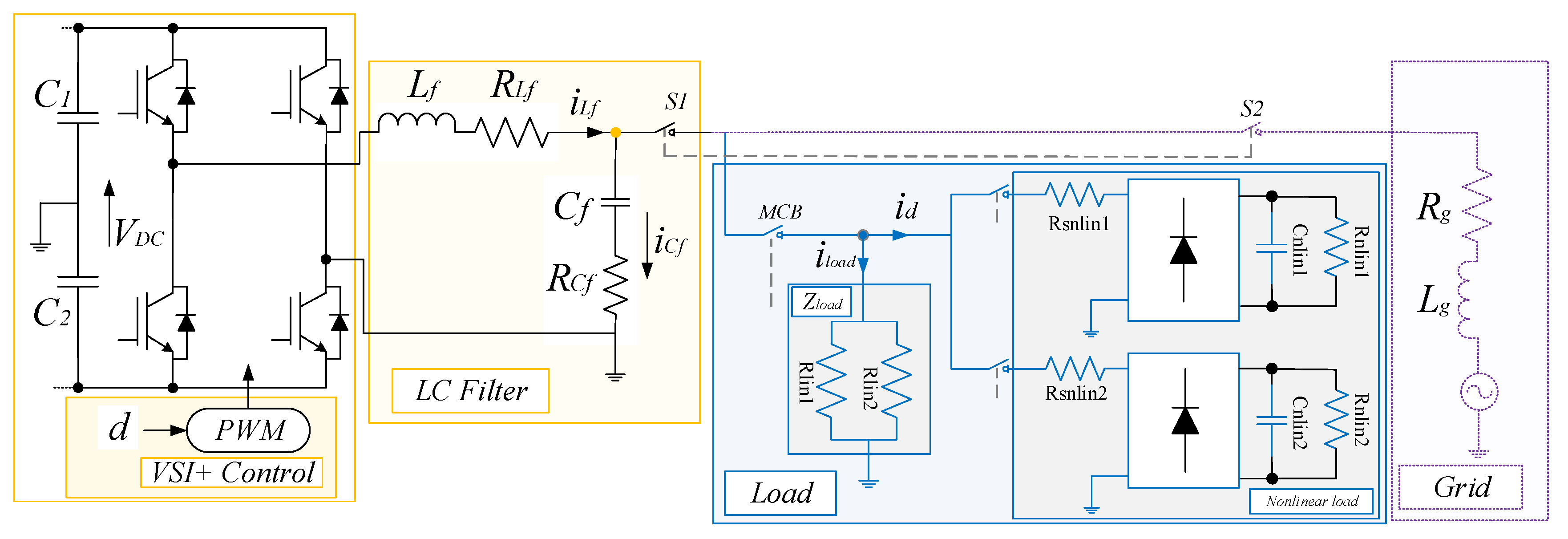
In the distributed energy system, the conditioning of the output voltage is performed by a DC-AC voltage inverter together with a second-order LC Low Pass filter, as shown in Figure 1. This figure shows the electrical diagram of the inverter used and the polarity of the currents involved. The model to be presented to the distributed energy system disregards the influence of the use of batteries and filter capacitors. The switching circuit (or switching) composed of the IGBT (Insulated Gate Bipolar Transistor) switches fed by the DC link voltage and the PWM (Pulse Width Modulation) modulator is modeled by the average value of the voltage applied to the LC low-pass filter and which will be represented by the input voltage , where is the gain of the modulator and the voltage of the DC link.
2.2. Linear Load Model Considerations
From Figure 1, the linear load model considers two fundamental factors that serve to understand the equations of modeling the DER system with a connected load.
- Considers the admittance as a time-varying parameter, where only the admittance values are known considering the two generic DER operating regimes: empty operation (minimum admittance) and nominal (maximum admittance).
- Considers current disturbances such as: sags, swell, notch or peak currents among other disturbances, and are modeled by the disturbance current [18]. The current is also an input to the DER system, but it is not controllable and its value will depend on the load, unlike the signal. In this way, the current is considered as a disturbance to the system and its presence is seen as a source of loss of system performance.
The load admittance value is in the range of , that is:
2.3. State Space Modelling of DER System
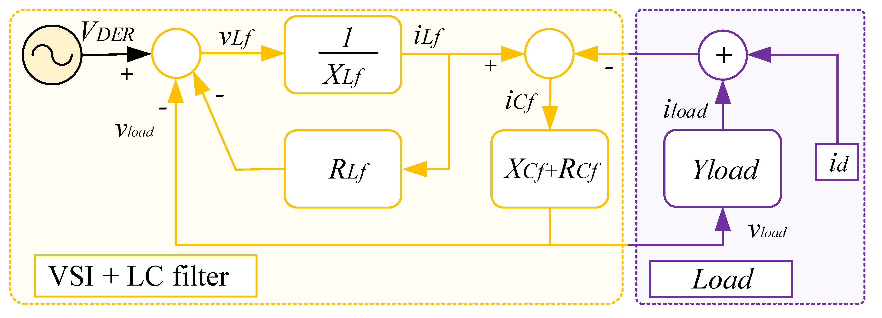
The representation of the system in the state space describes the dynamic behavior of all the energy storage elements in the distributed energy system, which in this case are the inductor and capacitor belonging to the inverter filter. To better understand the physical relationships between the components of the inverter, Figure 2 shows the block diagram representation of the inverter that shows the relationship between the capacitor voltage and the inductor current. The block diagram facilitates understanding and later description by state variables. As the load connected to the DER system can be linear or non-linear, this paper considers a representation of the load current in terms of two distinct components. The first current, derived from the admittance , which represents a linear load that consumes a current . The second added to is an current, which in this paper represents disturbances or disturbances to the value of the load applied to the distributed energy system. This current represents in a simplified way the model of non-linear loads connected to a DER system [19,20].
The initial methodology to compose the state matrices requires the determination of the differential equations that govern the behavior of the voltages and currents involved in the filter, according to the polarity defined in Figure 1. Basically, two equations are used, one referring to the mesh equation and the other one to the node equation as shown in (2).
Knowing that the relationship between voltage and current in the inductor and capacitor are given by:
The voltage drop in the internal resistance of the inductor is proportional to the current flowing through it, as well as the voltage drop in the internal resistance of the capacitor. In this way, Equation (4) is defined.
and taking into account the voltage drop in the resistance referring to the losses in the capacitor, we obtain:
From (3), the current is obtained at the series impedance of the capacitor, reaching the equation for voltage at the load:
We then arrive at an equation where there are only the measured variables related to each other as presented in (9).
As there is the presence of the capacitor voltage and its derivative, the following manipulation can be done to arrive at the first state Equation (10), related to the capacitor voltage.
Having obtained the first equation of state from the law of nodes applied to the system, the process for obtaining the second equation of state will now be started based on the law of meshes, given by Equation (11).
Using the study already carried out, the manipulation of the equation begins by substituting (3), and (4), leading expression (12).
Finally, Equation (16) comes from the state of the inductor current, which is extracted through the algebraic manipulation made in Equation (15).
Defining the current in the inductor as state and the voltage in the capacitor as another state, we obtain the following representation by the state variables:
where is the state vector, is the external disturbance signal, is the control signal (PWM output), is the output of the system, , and it is observed in the model, that the current is not a variable of known characteristic and is modeled as a disturbance external to the model.
3. Proportional Resonant Controller Model
In order to develop an effective control method to ensure the tracking of a sinusoidal reference, as well as the rejection of disturbances related to non-linear loads and harmonic compensation, new methodologies have been developed. In this work, proportional resonant controllers [21], based on the Internal Model Principle [22], are used. The proportional resonant compensators impose poles on the imaginary axis at frequencies equal to those of the reference, and show infinite gain in the resonance frequency. As real loads do not drain current linearly (with a waveform equal to the waveform of the applied voltage), the use of only one compensator at the fundamental frequency is not sufficient to keep a satisfactorily low THD. In particular, for DERs, typical non-linear loads can be seen as current disturbances in the frequency of the output voltage and in its multiples. The rejection of this type of disturbance will be fundamental for the good performance of a DER system. Consequently, a set of resonant compensators is used to reject each multiple harmonic frequency of the fundamental, by allocation of gain in multiple frequencies [23,24]. The following transfer function is usually used in the implementation of the ideal resonant controller.
where is the frequency of the signal to be followed or rejected. In some applications a damping factor is inserted at the poles of Equation (20) to avoid discrete implementation problems regarding the position of resonant poles at the edge of the unit circle [25]. Given a resonant controller with transfer function:
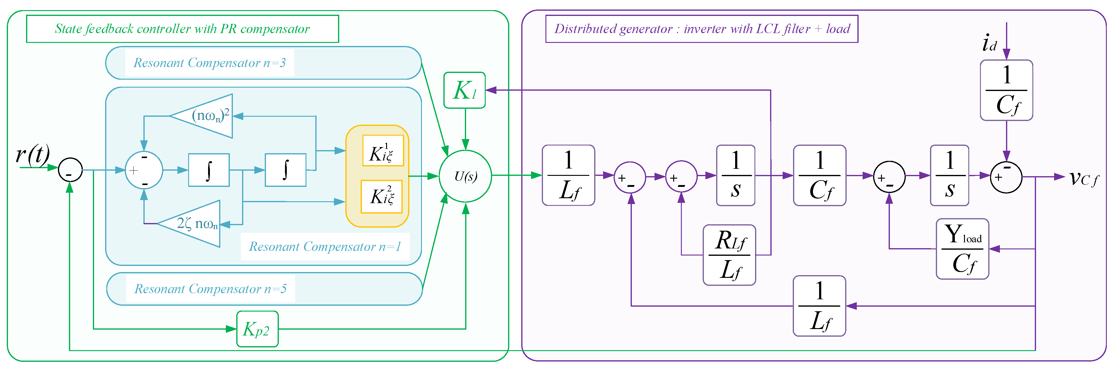
Note that by making the controller (21) reduces to (20). Controllers like this allocate imaginary pole pairs at the frequency of the reference to be traced and the frequencies of the disturbances to be rejected. To represent the multiple compensators, Equation (21) that models the resonant compensator in general is repeated in parallel in the block diagram of the control system, as shown in Figure 3. The multiple-resonant gain controller in (21) with proportional gain can be rewritten as
where and are the gains to be determined for each mode and is a direct transmission term applied to the input signal from the controller.
Controller Based on the Principle of the Internal
Model The design of controllers that guarantee follow-up of references and the rejection of disturbances is of great practical interest, being one of the main study topics for a number of authors over the years. The Principle of the Internal Model (IMP) [22] is an essential theoretical result for the design of a control system aiming at the follow-up of reference signals and rejection of disturbance signals. Its fundamental idea is to generate, within the control loop, a signal with the same characteristics as the signals to be followed and/or rejected. The closed-loop system must contain all persistent modes (which do not tend to zero at steady state) of the reference and disturbance signals in order to guarantee perfect tracking/rejection [26]. Using the principle of superposition, a controller based on the internal model principle simultaneously includes the reference and disturbance poles for the asymptotically stable system and without the cancellation of mentioned poles and zeros, the reference follow-up and rejection of disturbances with multiple harmonics, which occur in DERs with typical non-linear loads, with zero error in steady state. According to the principle of the internal model [22], in a feedback control system like the one in Figure 3, there is zero error in a steady state if the closed loop system is asymptotically stable and the poles of the system include the poles of reference to be tracked. In order to present the way in which the proportional resonant control tuning method was developed, initially it is necessary to obtain the state-space representation of the transfer function presented in Equation (22) [25,27], as in system (23):
The representation of (23) in the state space is given by
where is the state vector of the multi-resonant controller, is the input signal, is the output signal, and and are matrices of appropriate size.
for each resonant mode, that is, evaluated for each pair (), . The controller based on the internal model principle has internal variables as output variables, which facilitates the design of the controller gains by full state feedback, since all state variables are available for control, as shown in Figure 3. The augmented system is composed only of the plant and proportional compensators based on internal model principle in the frequency of the fundamental, , and the characteristic of rejection of load disturbances in the other harmonic frequencies. Generalizing the representation of the plant with the controller, it can be written that:
where
4. Robust Controller Design Based on LMIs
-Stability
The chosen -stability region is given by the intersection of a semi-plane sector () to guarantee a lower limit on settling time. Disc sector () is used as an upper limit on settling time. It restricts the magnitude of the eigenvalues indirectly and imposes a limitation on the control effort. LMI regions [28] are defined as regions of the complex plane that can be described in terms of characteristic functions as follows:
Lemma 1 below presents a condition that ensures the quadratic -stability of the closed loop system (26) in a given LMI region.
Lemma 1.
Quadratic stability of -Region [28]. Consider the LMI region with a characteristic function (28). Additionally, consider that , where both and are matrices with k lines and rank per complete line. The system (26) presents quadratic -stability with region (28) if there are real symmetric matrices and such that:
When the LMI region of interest is formed by the intersection of other LMI regions, quadratic -stability is guaranteed when the same matrix P meets (26) simultaneously with the characteristic functions of each region [29].
In particular, the region of our work can be described as , where
The following theorem details the conditions in the form of LMIs for the positioning of the eigenvalues of in
Remark.
One can notice that the quadratic -stability is wider than the condition. Indeed, the quadratic -stability allows to guarantee the stability of the uncertain system as well as the performance. We refer the interested reader to [28] and the references therein.
Theorem 1.
When real scalars σ and ρ are known, the closed-loop system is asymptotically stable for all and the poles are located in the region if there exists a symmetric positive definite matrices such that the following LMI are feasible:
With: He and He represent the hermitian block respectively.
5. Simulation Results and Discussion
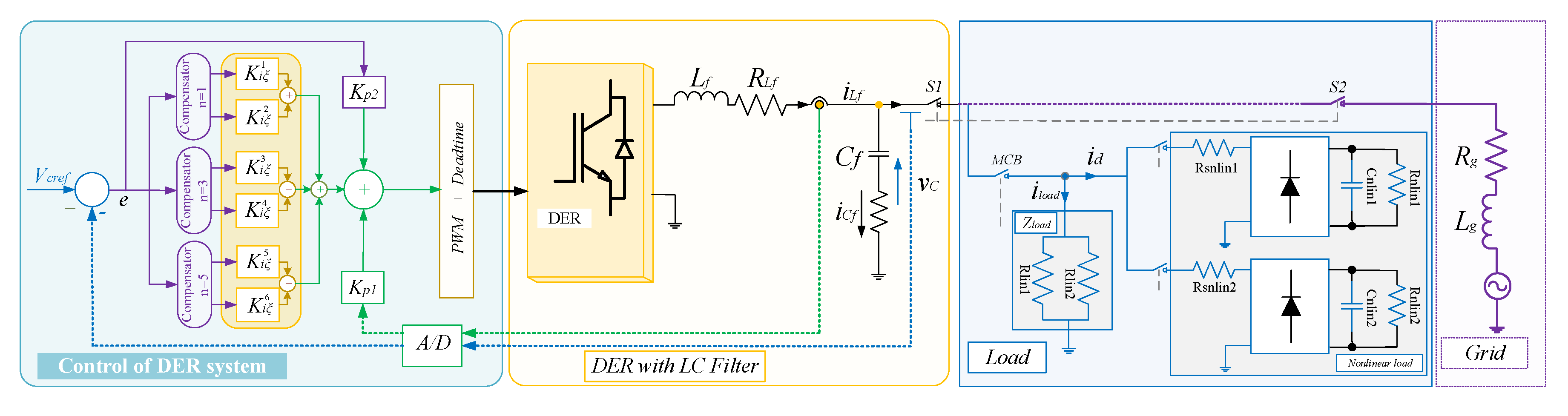
Using the robust control law presented in the previous sections for synthesizing gains of the distributed energy system, this section groups results from simulations tests. The numerical values of electrical components, LCL filter and resistances and capacitances parameters associated with each load situation for design purposes of the DER controller are listed in Table 1. The reference signal to be followed by the output voltage is sinusoidal with an RMS value of 127 V and frequency of 60 Hz. The inverter switching frequency is kHz, 360 times greater than the frequency of the reference signal. The simulation environment is given by Matlab/Simulink for the DER system with linear and non-linear test loads, including the generation of PWM signal for inverter switching in a half bridge and DER control loop, with a controller properly discretized by zero-order hold with a sampling frequency of kHz as shown in Figure 4. The LMI parameters chosen in this paper to improve the dynamic response and stability in steady-state are shown in Table 2.
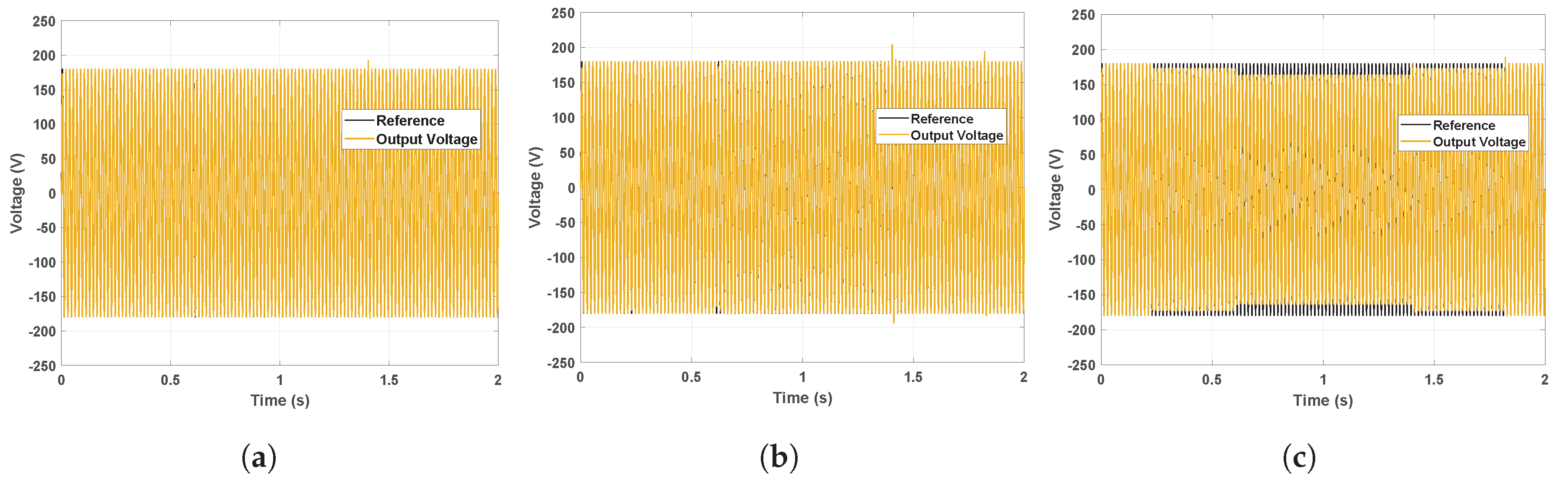
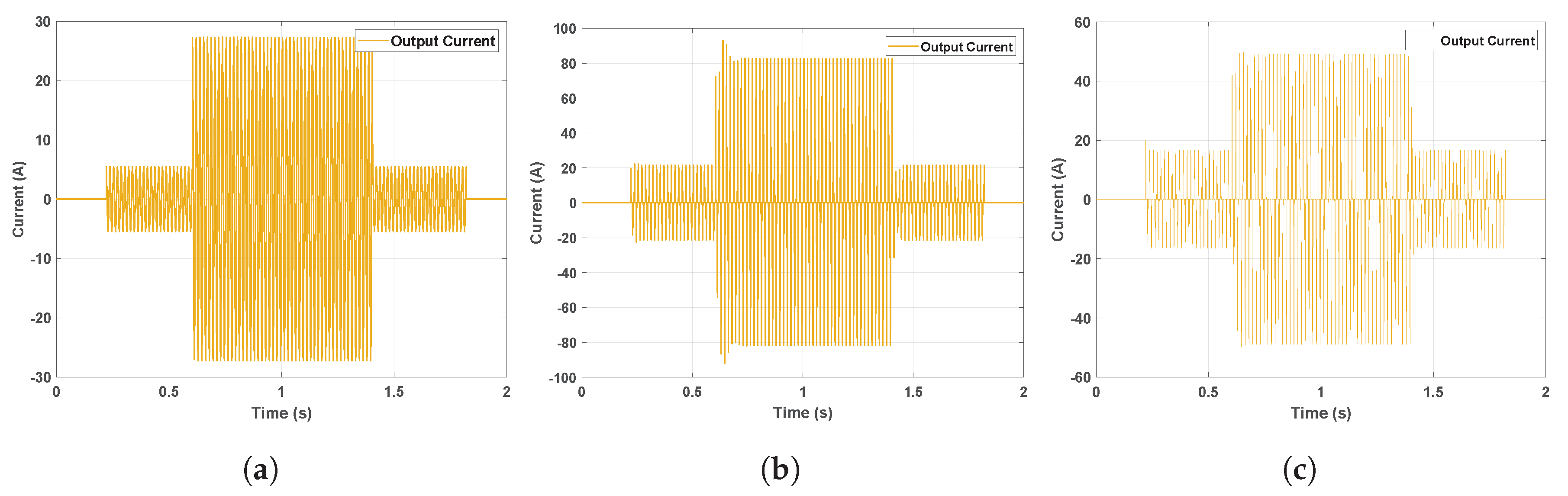
Figure 5 and Figure 6 show the voltage and current curve under load steps in the period of two seconds considering additional load steps of at s and of at s. Following by a subtractive step of at s and, finally, a subtractive step of at s. In Figure 5a, a cycle ( ms) of the voltage (127 V RMS) and output current (Figure 6a) of the DER system with linear load. In this figure it is evident how the voltage curve fits almost perfectly over the reference curve. Similarly for the current curve, which has an almost sinusoidal appearance with and without controller with fundamental frequency and a harmonics compensator (HC). Figure 5b and Figure 6b show voltage and output current curves from the DER system with non-linear load with HC, differently as for linear load, in non-linear load, the deformation of the current curve is more pronounced, which is caused by this type of load. Figure 5c and Figure 6c show the simulation results for voltage and current without HC in the controller; from these figures we can seen that the non-linear load creates a voltage deviation voltage that increases proportionally to the connected step load. In the linear and non-linear load with HC, the shape of the current is slightly deformed compared with non-linear load without HC. However, both non-linear loads present small transients and overshoots for additive and subtractive load steps contrary to the linear load, which has voltage and current responses that are perfectly sinusoidal.
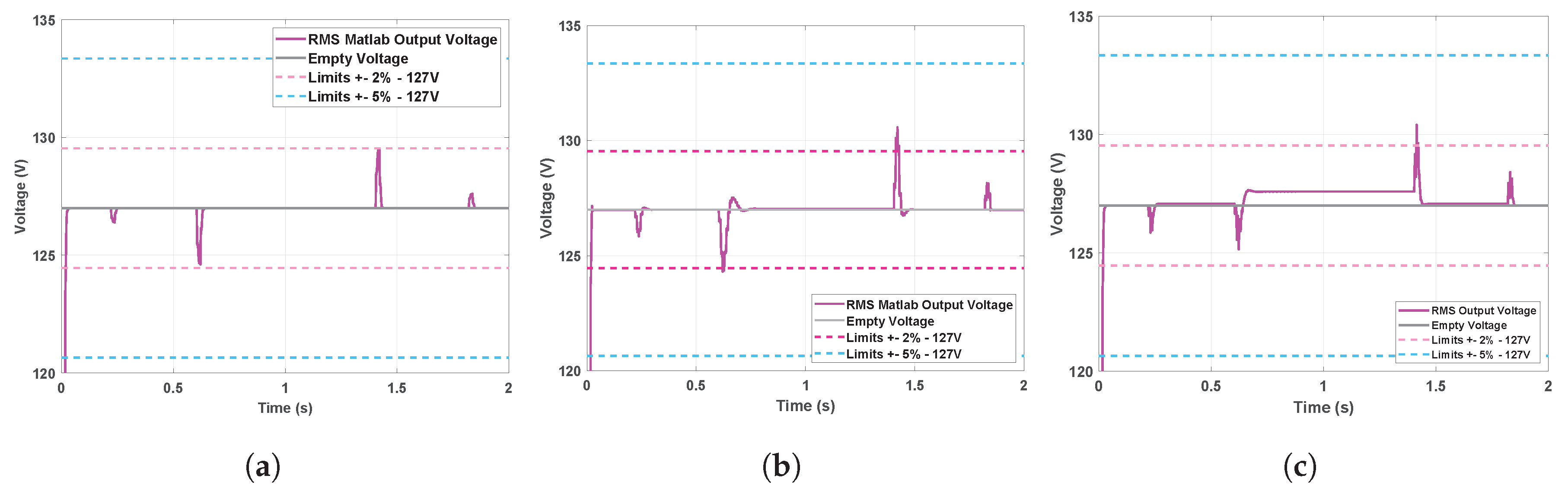
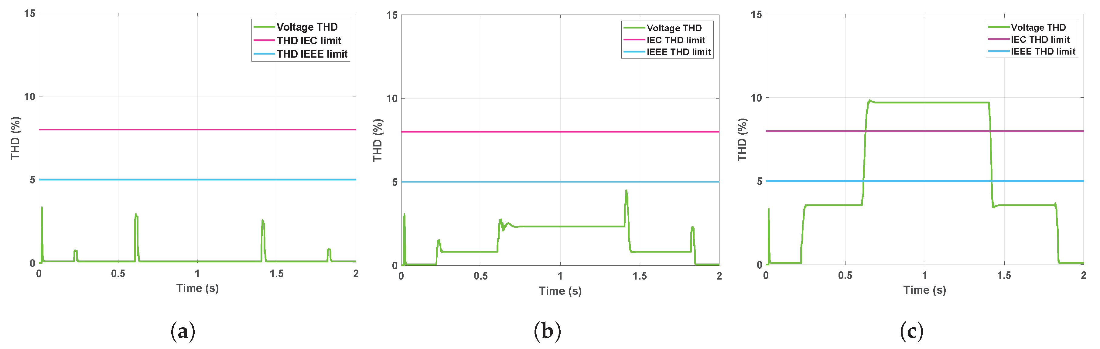
Figure 7 shows the values of the empty RMS voltage, with and linear load, and with and non-linear load, respectively, of the DER system. In this study, we take account of the steady state voltage without the transients of connected and disconnected loads. For the linear load, we observe that the RMS value of the voltage remains satisfying the most stringent standard, which is also the case for the non-linear load with the controller use HC. However, for the non-linear load without HC, when the addition of non-linear load occurs, the RMS value of the voltage slightly exceeds () the limit of the IEEE 944 standard. Figure 8 shows the THD of the DER system output voltage for all additive and subtractive steps with different periods for linear and non-linear loads. In the cases where the PR controllers are used with harmonic compensators, the THD with and linear/non-linear loads varying meet the IEEE and IEC standards for the proposed LMI approaches, as shown in Figure 8a,b. However, when the PR controllers are used without harmonic compensators, the THD with non-linear load satisfied the IEC 62040-3 standard and IEEE 944 standard norms but did not satisfy the norms with non-linear load. For each case, the THD values of the DER system with empty, with and linear/non-linear load are shown in Table 3.
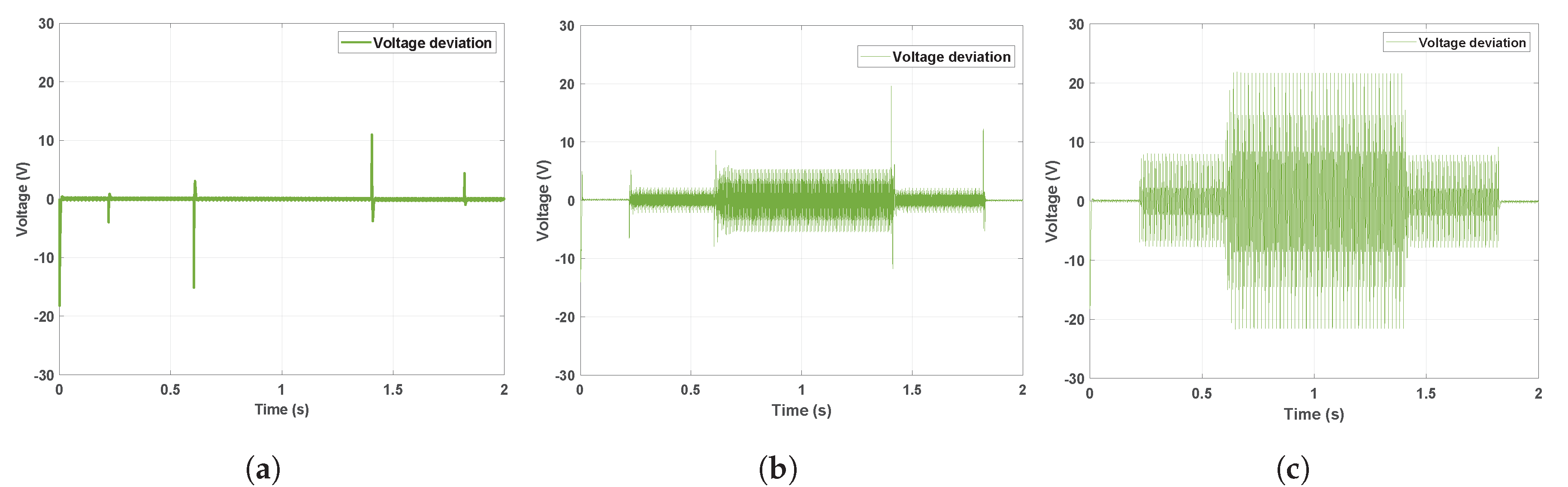
It is observed in Figure 9a–c that the system is running empty and, when the step non-linear load increases (with and without HC in controller), the voltage deviation increases, which confirms the results shown in Figure 5. The increasing of voltage deviation is more important when not using a harmonics compensator in the controller. However, when the system undergoes a subtraction of the non-linear load step, the voltage deviation decreases. It is important to note that this graph does not take into account load insertion or removal transients. Our interest in this case in assessing this graph is the voltage in steady state. However, it is possible to observe that transients appear in the voltage deviation value due to the loads connection/disconnection. These transients do not impact the proposed control system performance because of the output voltages’ small variation in the amplitude and the fast recovery time. In fact, transients remain in compliance with IEEE 944 standard limits.
6. Conclusions
The distributed generation resource systems are being used in the micro-grid applications and, therefore, the concern with their reliability grows as the currents requested from DER systems have a non-linear character. In this paper, a multiple resonant compensator strategy through the robust control theory is proposed for guaranteeing stability and performance for different types of loads including the problem of harmonic cancellation and attenuation of disturbances in the output voltage of DER systems caused by non-linear loads. The stability and performance criteria based on Lyapunov’s theory are used and described using the formulation by linear matrix inequalities, where it was possible to establish design criteria for determining the gains of the multiple resonant compensators by allocating poles in order to guarantee a good dynamic performance and harmonic rejection. The simulation results prove that the controller studied in this work presents advantages in relation to the dynamic performance and in a steady state against load variations. In future work, an adaptive frequency system will be added to resonant compensators to increase robustness when a variation in the frequency of the reference signal is allowed. Another important point is to use Anti Windup compensators in parallel with the resonant to avoid saturation of the control signal.
Author Contributions
Conceptualization, A.E.M.B., M.Z., S.B.E. and M.B.; Methodology, A.E.M.B., M.Z., S.B.E. and M.B.; Software, A.E.M.B.; Validation, A.E.M.B., M.Z., S.B.E. and M.B.; Formal Analysis, A.E.M.B., M.Z., S.B.E., K.B. and M.B.; Investigation, A.E.M.B.; Writing—Original Draft Preparation, A.E.M.B.; Writing—Review & Editing, A.E.M.B., M.Z., S.B.E., K.B. and M.B. All authors have read and agreed to the published version of the manuscript.
Funding
This research received no external funding.
Conflicts of Interest
The authors declare no conflict of interest.
References
- Zia, M.F.; Elbouchikhi, E.; Benbouzid, M.; Guerrero, J.M. Microgrid Transactive Energy Systems: A Perspective on Design, Technologies, and Energy Markets. In Proceedings of the IECON 2019—45th Annual Conference of the IEEE Industrial Electronics Society, Lisbon, Portugal, 14–17 October 2019; Volume 1, pp. 5795–5800. [Google Scholar]
- Zia, M.F.; Benbouzid, M.; Elbouchikhi, E.; Muyeen, S.M.; Techato, K.; Guerrero, J.M. Microgrid Transactive Energy: Review, Architectures, Distributed Ledger Technologies, and Market Analysis. IEEE Access 2020, 8, 19410–19432. [Google Scholar] [CrossRef]
- Bouzid, A.M.; Chériti, A.; Sicard, P. H-infinity loopshaping controller design of micro-source inverters to improve the power quality. In Proceedings of the 2014 IEEE 23rd International Symposium on Industrial Electronics (ISIE), Istanbul, Turkey, 1–4 June 2014; pp. 2371–2378. [Google Scholar]
- Eltawil, M.A.; Zhao, Z. Grid-connected photovoltaic power systems: Technical and potential problems—A review. Renew. Sustain. Energy Rev. 2010, 14, 112–129. [Google Scholar] [CrossRef]
- Timbus, A.; Liserre, M.; Teodorescu, R.; Rodriguez, P.; Blaabjerg, F. Evaluation of current controllers for distributed power generation systems. IEEE Trans. Power Electron. 2009, 24, 654–664. [Google Scholar] [CrossRef]
- Bouzid, A.M.; Golsorkhi, M.S.; Sicard, P.; Chériti, A. H∞ structured design of a cascaded voltage/current controller for electronically interfaced distributed energy resources. In Proceedings of the 2015 Tenth International Conference on Ecological Vehicles and Renewable Energies (EVER), Monte Carlo, Monaco, 31 March–2 April 2015; pp. 1–6. [Google Scholar]
- Samavati, E.; Mohammadi, H. Simultaneous voltage and current harmonics compensation in islanded/grid-connected microgrids using virtual impedance concept. Sustain. Energy Grids Netw. 2019, 20, 100258. [Google Scholar] [CrossRef]
- Husev, O.; Roncero-Clemente, C.; Makovenko, E.; Pimentel, S.P.; Vinnikov, D.; Martins, J. Optimization and Implementation of the Proportional-Resonant Controller for Grid-Connected Inverter With Significant Computation Delay. IEEE Trans. Ind. Electron. 2020, 67, 1201–1211. [Google Scholar] [CrossRef]
- Osório, C.R.D.; Koch, G.G.; Pinheiro, H.; Oliveira, R.C.L.F.; Montagner, V.F. Robust Current Control of Grid-Tied Inverters Affected by LCL Filter Soft-Saturation. IEEE Trans. Ind. Electron. 2019, 67, 6550–6561. [Google Scholar] [CrossRef]
- Ye, T.; Dai, N.; Lam, C.; Wong, M.; Guerrero, J.M. Analysis, Design, and Implementation of a Quasi-Proportional-Resonant Controller for a Multifunctional Capacitive-Coupling Grid-Connected Inverter. IEEE Trans. Ind. Appl. 2016, 52, 4269–4280. [Google Scholar] [CrossRef]
- Khalfalla, H.; Ethni, S.; Al-Greer, M.; Pickert, V.; Armstrong, M.; Phan, V.T. An adaptive proportional resonant controller for single phase PV grid connected inverter based on band-pass filter technique. In Proceedings of the 2017 11th IEEE International Conference on Compatibility, Power Electronics and Power Engineering (CPE-POWERENG), Cadiz, Spain, 4–6 April 2017; pp. 436–441. [Google Scholar]
- Kumar, N.; Saha, T.K.; Dey, J. Control, implementation, and analysis of a dual two-level photovoltaic inverter based on modified proportional-resonant controller. IET Renew. Power Gener. 2018, 12, 598–604. [Google Scholar] [CrossRef]
- Saim, A.; Houari, A.; Guerrero, J.M.; Djerioui, A.; Machmoum, M.; Ahmed, M.A. Stability Analysis and Robust Damping of Multiresonances in Distributed-Generation-Based Islanded Microgrids. IEEE Trans. Ind. Electron. 2019, 66, 8958–8970. [Google Scholar] [CrossRef]
- Bouzid, A.E.M.; Sicard, P.; Chaoui, H.; Cheriti, A. Robust three degrees of freedom based on H∞ controller of voltage/current loops for DG unit in micro grids. IET Power Electron. 2019, 12, 1413–1424. [Google Scholar] [CrossRef]
- Bouzid, A.M.; Sicard, P.; Chériti, A.; Bouhamida, M. H∞ loopshaping controller design of micro-source inverters. In Proceedings of the 2014 IEEE 27th Canadian Conference on Electrical and Computer Engineering (CCECE), Toronto, ON, Canada, 4–7 May 2014; pp. 1–6. [Google Scholar]
- Zerrougui, M.; Darouach, M.; Boutat-Baddas, L.; Souley-Ali, H. H∞ filtering for singular bilinear systems with application to a single-link flexible-joint robot. Int. J. Control Autom. Syst. 2014, 12, 590–598. [Google Scholar] [CrossRef]
- Zemouche, A.; Zerrougui, M.; Boulkroune, B.; Rajamani, R.; Zasadzinski, M. A new LMI observer-based controller design method for discrete-time LPV systems with uncertain parameters. In Proceedings of the 2016 American Control Conference (ACC), Boston, MA, USA, 6–8 July 2016; pp. 2802–2807. [Google Scholar]
- Thirumala, K.; Pal, S.; Jain, T.; Umarikar, A.C. A classification method for multiple power quality disturbances using EWT based adaptive filtering and multiclass SVM. Neurocomputing 2019, 334, 265–274. [Google Scholar] [CrossRef]
- Bouzid, A.M.; Sicard, P.; Paquin, J.; Yamane, A. A robust control strategy for parallel-connected distributed generation using real-time simulation. In Proceedings of the 2016 IEEE 7th International Symposium on Power Electronics for Distributed Generation Systems (PEDG), Vancouver, BC, Canada, 27–30 June 2016; pp. 1–8. [Google Scholar]
- Bouzid, A.E.M.; Sicard, P.; Chaoui, H.; Cheriti, A.; Sechilariu, M.; Guerrero, J.M. A novel decoupled trigonometric saturated droop controller for power sharing in islanded low-voltage microgrids. Electr. Power Syst. Res. 2019, 168, 146–161. [Google Scholar] [CrossRef]
- Fukuda, S.; Yoda, T. A novel current-tracking method for active filters based on a sinusoidal internal model [for PWM invertors]. IEEE Trans. Ind. Appl. 2001, 37, 888–895. [Google Scholar] [CrossRef] [Green Version]
- Francis, B.A.; Wonham, W.M. The internal model principle for linear multivariable regulators. Appl. Math. Optim. 1975, 2, 170–194. [Google Scholar] [CrossRef]
- Zmood, D.N.; Holmes, D.G. Stationary frame current regulation of PWM inverters with zero steady-state error. IEEE Trans. Power Electron. 2003, 18, 814–822. [Google Scholar] [CrossRef]
- Teodorescu, R.; Blaabjerg, F.; Liserre, M.; Loh, P.C. Proportional-resonant controllers and filters for grid-connected voltage-source converters. IEE Proc. Electr. Power Appl. 2006, 153, 750–762. [Google Scholar] [CrossRef] [Green Version]
- Pereira, L.F.A.; Flores, J.V.; Bonan, G.; Coutinho, D.F.; da Silva, J.M.G. Multiple resonant controllers for uninterruptible power supplies—A systematic robust control design approach. IEEE Trans. Ind. Electron. 2013, 61, 1528–1538. [Google Scholar] [CrossRef]
- Callier, F.M.; Desoer, C.A. Linear System Theory; Springer Science & Business Media: Berlin, Germany, 2012. [Google Scholar]
- Maccari, L.A.; Massing, J.R.; Schuch, L.; Rech, C.; Pinheiro, H.; Oliveira, R.C.L.F.; Montagner, V.F. LMI-Based Control for Grid-Connected Converters With LCL Filters Under Uncertain Parameters. IEEE Trans. Power Electron. 2014, 29, 3776–3785. [Google Scholar] [CrossRef]
- Chilali, M.; Gahinet, P.; Apkarian, P. Robust pole placement in LMI regions. IEEE Trans. Autom. Control 1999, 44, 2257–2270. [Google Scholar] [CrossRef] [Green Version]
- Gahinet, P. H∞ Design with Pole Placement Constraints: An LMI approach. IEEE Trans. Autom. Control 1996, 45, 358–367. [Google Scholar]
Figure 1.
Distributed energy system circuit.

Figure 2.
Inverter block diagram with filter and load.

Figure 3.
Block diagram of closed loop system for proportional resonant controller and inverter with LCL filter.
Figure 3.
Block diagram of closed loop system for proportional resonant controller and inverter with LCL filter.

Figure 4.
General scheme of the distributed energy resource (DER) system with the proposed control.

Figure 5.
DER output voltage curve different loads. (a) 100% linear load with HC. (b) 100% non-linear load with HC. (c) 100% non-linear load without harmonics compensator (HC).
Figure 5.
DER output voltage curve different loads. (a) 100% linear load with HC. (b) 100% non-linear load with HC. (c) 100% non-linear load without harmonics compensator (HC).

Figure 6.
DER system output current curve. (a) 100% linear load with HC. (b) 100% non-linear load with HC. (c) 100% non-linear load without HC.
Figure 6.
DER system output current curve. (a) 100% linear load with HC. (b) 100% non-linear load with HC. (c) 100% non-linear load without HC.

Figure 7.
RMS value of DER system output voltage. (a) 100% linear load with HC. (b) 100% non-linear load with HC. (c) 100% non-linear load without HC.
Figure 7.
RMS value of DER system output voltage. (a) 100% linear load with HC. (b) 100% non-linear load with HC. (c) 100% non-linear load without HC.

Figure 8.
THD value of DER system output voltage. (a) 100% linear load with HC. (b) 100% non-linear load with HC. (c) 100% non-linear load without HC.
Figure 8.
THD value of DER system output voltage. (a) 100% linear load with HC. (b) 100% non-linear load with HC. (c) 100% non-linear load without HC.

Figure 9.
DER system output voltage deviation. (a) 100% linear load with HC. (b) 100% non-linear load with HC. (c) 100% non-linear load without HC.
Figure 9.
DER system output voltage deviation. (a) 100% linear load with HC. (b) 100% non-linear load with HC. (c) 100% non-linear load without HC.


Table 1.
DER system parameters.
| Parameter | Value |
|---|---|
| Nominal power | |
| RMS output voltage | |
| Frequency | |
| Output power factor | |
| Inductance | |
| Parasitic resistance of the inductor | |
| Capacitance | |
| Capacitive parasitic resistance (considered) | |
| Uncertain linear load impedance | |
| DC bus capacitances | |
| DC bus voltage | |
| Load parameters | |
| , |
Table 2.
Linear matrix inequalities (LMI) parameters used for controller design.
| Parameter | Value |
|---|---|
| (Sigma position) | 100 |
| (radius of the circle) | 20,000 |
| c (center of circle) | 0 |
Table 3.
THD voltage with different load steps.
| Operation Mode | Empty | Load 20% | Load 100% |
|---|---|---|---|
| Linear load | 0.09% | 0.088% | 0.087% |
| Non-linear load with HC | 0.062% | 0.8107% | 2.328% |
| Non-linear load without HC | 0.12% | 3.547% | 9.71% |
Publisher’s Note: MDPI stays neutral with regard to jurisdictional claims in published maps and institutional affiliations. |
© 2020 by the authors. Licensee MDPI, Basel, Switzerland. This article is an open access article distributed under the terms and conditions of the Creative Commons Attribution (CC BY) license (http://creativecommons.org/licenses/by/4.0/).
Share and Cite
MDPI and ACS Style
Bouzid, A.E.M.; Zerrougui, M.; Ben Elghali, S.; Beddiar, K.; Benbouzid, M. Robust Resonant Controllers for Distributed Energy Resources in Microgrids. Appl. Sci. 2020, 10, 8905. https://doi.org/10.3390/app10248905
AMA Style
Bouzid AEM, Zerrougui M, Ben Elghali S, Beddiar K, Benbouzid M. Robust Resonant Controllers for Distributed Energy Resources in Microgrids. Applied Sciences. 2020; 10(24):8905. https://doi.org/10.3390/app10248905
Chicago/Turabian StyleBouzid, Allal El Moubarek, Mohamed Zerrougui, Seifeddine Ben Elghali, Karim Beddiar, and Mohamed Benbouzid. 2020. "Robust Resonant Controllers for Distributed Energy Resources in Microgrids" Applied Sciences 10, no. 24: 8905. https://doi.org/10.3390/app10248905
Note that from the first issue of 2016, this journal uses article numbers instead of page numbers. See further details here.