Article

Three-Dimensional Combined Finite-Discrete Element Modeling of Shear Fracture Process in Direct Shearing of Rough Concrete–Rock Joints

1
Department of Mineral Resources and Energy Engineering, Jeonbuk National University, Jeonju-si 54896, Korea
2
Faculty of Engineering, Hokkaido University, Hokkaido 060-8628, Japan
3
Korea Institute of Civil Engineering and Building Technology, Goyang-si 10223, Korea
4
School of Engineering, College of Science and Engineering, University of Tasmania, Sandy Bay, TAS 7001, Australia
*
Authors to whom correspondence should be addressed.
Appl. Sci. 2020, 10(22), 8033; https://doi.org/10.3390/app10228033
Submission received: 12 October 2020 / Revised: 30 October 2020 / Accepted: 4 November 2020 / Published: 12 November 2020
(This article belongs to the Special Issue Fracture Mechanics – Theory, Modeling and Applications)

Abstract

:
A three-dimensional combined finite-discrete element element method (FDEM), parallelized by a general-purpose graphic-processing-unit (GPGPU), was applied to identify the fracture process of rough concrete–rock joints under direct shearing. The development process of shear resistance under the complex interaction between the rough concrete–rock joint surfaces, i.e., asperity dilatation, sliding, and degradation, was numerically simulated in terms of various asperity roughness under constant normal confinement. It was found that joint roughness significantly affects the development of overall joint shear resistance. The main mechanism for the joint shear resistance was identified as asperity sliding in the case of smoother joint roughness and asperity degradation in the case of rougher joint asperity. Moreover, it was established that the bulk internal friction angle increased with asperity angle increments in the Mohr–Coulomb criterion, and these results follow Patton’s theoretical model. Finally, the friction coefficient in FDEM appears to be an important parameter for simulating the direct shear test because the friction coefficient affects the bulk shear strength as well as the bulk internal friction angle. In addition, the friction coefficient of the rock–concrete joints contributes to the variation of the internal friction angle at the smooth joint than the rough joint.

1. Introduction

In a ground-anchored suspension bridge, the anchorage performs the function of supporting the tension force acting on the main cable. As one of the construction methods of anchorage, gravity-type anchorage (GTA) (see Figure 1) is widely used due to a variety of advantages such as simple mechanical configuration, ease of construction, and its vast applications [1]. The GTA resists the cable load via the weight of the anchorage structure itself, and this depends on the frictional resistance between the anchorages (concrete) and the foundation (rock). For designing the GTA, many guidelines are recommended to assess the stability of a GTA using the gravity method [2,3,4,5,6], and it is coupled with the Mohr–Coulomb (M-C) criterion, which is defined by several parameters such as friction angle and cohesion. However, some guidelines assume the M-C parameters to be a conservative constant value (e.g., c = 0 and t a n ϕ   =   0.6 ) [5,6] in the vicinity of the joint between the anchorage and the foundation. The rough geometry of the joint is also neglected in the gravity method. Such oversimplifications related to joint properties may lead to a conservative stability analysis, and it may require a huge amount of earth and rock excavation and concrete consumption, which may result in high construction costs and environmental damage in GTA. Therefore, it is crucial to extensively investigate the frictional resistance and failure behaviors around the joint structure between concrete and rock surfaces (i.e., concrete–rock joint) with rough geometry under shearing.
The problem of the failure of the concrete–rock (C-R) joint under shearing has been considered as a special case of the failure of rock mass containing rough joint surfaces (i.e., rock–rock joint) under shearing. The problem of rock–rock (R-R) joints subjected to shearing has been investigated extensively, and several models for this problem have been proposed [7,8,9,10,11,12,13,14,15,16,17,18,19,20,21,22,23,24,25,26]. These studies have examined the major factors that affect the behavior of the R-R joint, considering the rock mass properties around the rock joint, joint surface roughness, and boundary conditions applicable to joints, and some useful solutions have been proposed.
Based on the research and knowledge regarding the shear behavior of the R-R joints, several investigations of the interaction of C-R joint surfaces have been performed by researchers through direct shear tests on the C-R joints under constant normal loading (CNL) and constant normal stiffness (CNS) conditions. Thomas et al. [11] performed a direct shear test on regular triangular C-R joint surfaces under several CNS conditions. As an extension of their study, Johnson et al. [12] proposed analytical solutions to predict the development of the shear resistance in rock-socketed concrete piles, which can be idealized as a C-R joint problem under CNS conditions. Kodikara and Johnston [27] investigated the shear behavior of C-R joints with irregular triangle asperities, and they compared the obtained results with the case of regular triangular asperities. They revealed that the major difference between irregular and regular asperities is in the fact that an irregular joint presents more ductile behavior than a regular joint does. Similarly, Gu et al. [28] carried out a direct shear test with fractal profiles under several CNL conditions, and the results were compared with a case of regular triangular asperity. The response of the joint with fractal profiles showed more ductile behavior and presented a significantly lower peak overall strength than the case with regular asperity, because each single asperity in the fractal profile was progressively fractured rather than simultaneously fractured. Saiang et al. [29] investigated the shear behavior of a bonded shotcrete–rock joint. They found that for the development of the overall shear strength of the joint, the cohesive strength of the joint played an important role when the applied normal stress confinement was fairly low (0.2~0.5 MPa), while the friction was more important under higher normal stress confinement.
Based on experimental observation and theoretical analysis, several constitutive models have also been developed. Seidel and Haberfield [30] developed a constitutive model to predict the mechanism of the development of overall shear strength of the C-R joint. This constitutive model simulated important physical processes including asperity sliding, asperity shearing, and post-peak behavior of the concrete–rock joint. However, Harberfield and Johnston [31] have pointed out the limitations of existing empirical and analytical approaches. The obtained results posted significant dependencies on specific experimental site and test conditions for the existing empirical models, while the requirements of complex input parameters and oversimplifications showed difficulty in terms of the applicability of existing analytical approaches. As a result, they proposed a new theoretical model that can describe the main mechanism and requires joint roughness, basic rock properties, and boundary conditions for the cases of R-R and C-R joints. However, these constitutive models still could not have investigated the process of asperity degradation and shear fracturing during a direct shear test, indicating that the empirical-based and theoretical-based approaches suffer from significant limitations in their applications.
The viability of continuum and discontinuum-based numerical methods to numerically simulate the shear behavior of R-R and C-R joints has advanced alongside computational geomechanics technology. Tian et al. [32] used a three-dimensional (3D) FEM to develop a cohesive interface model of cemented C-R joints and simulated a direct shear test with a smooth joint surface. Using the discrete element method (DEM), Bahaaddini et al. [33] simulated the shear behavior of rock joints using the bonded particle model (BPM), which is available in the two-dimensional (2D) particle flow code (PFC2D). They modeled the shear behavior of a saw-tooth triangular bonded and unbonded R-R joint and considered the joint roughness coefficient (JRC) profiles [7] as they investigated the rock damage process during a direct shear test. Ultimately, they successfully simulate the propagation of tensile cracks and the asperity crushing. Using the BPM of the 3D particle flow code (PFC3D), Park and Song [34] modeled a series of direct shear tests with rock–rock joints and investigated the effect of the geometrical topology and the micro-properties of the joints on shear behavior. Although the DEM with the BPM successfully modeled the fracture asperity and gouges, this method required a more tedious calibration process to acquire the unknown micro-parameters until the response of the macro-scale model accorded with the laboratory test results rather than the FEM application. Many of the computational resources also accompany simulating the crack propagation of the rock and concrete than the FEM.
Recently, the combined finite-discrete element method (FDEM), originally proposed by Munjiza [35,36], has attracted significant attention in the field of computational solid mechanics. Since then, various FDEM codes have been developed in several research groups across the world [37,38,39,40,41,42,43,44,45,46,47,48,49,50,51,52,53,54]. The FDEM can model the three important aspects of solid fracture, i.e., the continuous deformation in the intact regime, the transition from continuum to discontinuum, and the very complex contact mechanics between solid surfaces, including newly created macroscopic fracture surfaces. For this reason, the FDEM is expected to model the three-dimensionally complex asperity degradation and shear resistance process, and thus, this study employed the FDEM.
FDEM has been applied to the investigation of the fracture process in the direct shearing of the R-R joints. For example, Karami and Stead [53] utilized 2D FDEM implemented in ELFEN software to investigate the process of the R-R joint degradation during direct shear tests with various joint roughness under different normal stress. Similarly, Liu et al. [46] applied the 2D FDEM implemented in the Y-HFDEM IDE code to simulate the direct shearing process of rock with rough R-R joints under various dynamic loading and investigated the effect of different patterns of asperity roughness. They successfully simulated the development process of overall shear resistance including asperity sliding, asperity degradation, gouge formation, and gouge grinding. Furthermore, Tatone and Grasselli [54] implemented the simulation of a direct shear test using the 2D FDEM implemented in Y-Geo code for a 2D profiled rock–rock joint in which the detailed joint topology was extracted from the 3D discontinuity surface data obtained from the micro-CT scanning system, and the simulation results of the direct shear test presented a good agreement with laboratory observations over the first 2–3 mm of shear displacement. According to these application examples, the FDEM has great capabilities for detailed investigations of complex fracture processes in the shear test of R-R joints. However, all the previous research using FDEM was limited to 2D problems and R-R joint problems. In addition, in the experience of the author, the heterogeneous fracturing was shown in a laboratory direct shear test of the concrete–rock joint specimen with uniform and rough tooth-saw-shaped asperity. Therefore, to achieve a better understanding of the development of resistance mechanisms in the C-R joints under shearing, 3D numerical simulation of the fracturing process of concrete and rock around the C-R joints is necessary, because the concrete and rock are fractured involving complex 3D processes. However, no previous research has been reported for the application of 3D FDEM to the investigation of the direct shear test of the rough C-R joint under shearing.
In relation to the work summarized above, this paper aims to apply the 3D FDEM to investigate the detailed development of resistance mechanisms in a direct shear test of a rough C-R joint under shearing including asperity dilatation, asperity sliding, and asperity degradation behavior. The organization of this paper is as follows: Section 2 briefly introduced the 3D FDEM implemented in the Y-HFDEM integrated development environment (IDE) whose computational performance has been greatly improved by the introduction of parallel computation utilizing general-purpose-graphic-processing-unit (GPGPU). In Section 3, calibration of the input parameters for the 3D FDEM simulations in Section 4 was first conducted against the experimental results of the target rock and concrete through the uniaxial compressive strength (UCS) and Brazilian tensile strength (BTS) tests. Using calibrated input parameters, a direct shear test of the rough C-R joint was investigated in detail using 3D FDEM. Finally, the authors discuss the effect of the roughness of asperity as well as the effect of friction coefficient on friction resistance during direct shear development.

2. GPGPU-Parallelized 3D Y-HFDEM IDE

In this study, an FDEM implemented in 3D Y-HFDEM IDE code was applied to simulate the fracturing of a direct shear test of a rough concrete–rock joint under shearing. Originally, the code was developed using the object-oriented programming tool (i.e., Visual C++) [44,45,46], and it was based on non-parallelized open-source Y-2D/3D libraries with OpenGL [36,37,38]. Using this code, the various rock engineering problems have been successfully solved by simulating rock fracturing [44,45,46]. However, due to the non-parallelized nature of the code, its previous applications were limited to small-scale 2D problems using relatively rough meshes. Recently, to overcome these limitations, a parallel programming scheme using GPGPU controlled by compute unified device architecture (CUDA) C/C++ was incorporated to develop the GPGPU-parallelized Y-HFDEM IDE code by the authors [47,48,49,50,51] for 2D and 3D FDEM modeling. Since the full details of the Y-HFDEM IDE code can be found in the literature [49,50], we focus in this section on the essential parts of the 3D FDEM in order to model the fracture process in the direct shearing of the rough concrete–rock joint. In the remaining sections of this paper, the 3D FDEM implemented in the GPGPU-parallelized Y-HFDEM 3D IDE code is simply called the 3D FDEM.
In the 3D FDEM, the continuous, i.e., elastic, deformations of rock and concrete are modeled using continuum solid elements (i.e., 4-noded tetrahedral elements, TET4s) [50].
The fracturing in the rock and concrete are modeled by an intrinsic cohesive zone model (ICZM) with the concept of smeared crack [55] representing opening and sliding cracks as well as mixed-mode I–II fracturing. In this model, 6-node initially zero-thickness cohesive elements (CE6) are inserted into all the boundaries of the TET4s at the beginning of the FDEM simulation to model the fracture of the rock and concrete (Figure 2). The opening and sliding of the faces in each CE6 are governed by tensile and shear softening curves as a function of the crack opening ( w o ) and sliding displacements ( w s ) (Figure 3). In the tensile and shear softening curves, the normal and shear cohesive tractions (i.e., σ coh and τ coh , respectively) acting on each side of CE6 are calculated using Equations (1) and (2), respectively:
σ c o h = 2 w o w o o v e r l a p T s i f   w o < 0 2 w o w o p w o w o p 2 f ( D ) T s i f   0 w o w o p f ( D ) T s i f   w o p < 0
τ c o h = 2 w s w s p w s w s p 2 ( σ c o h tan ( ϕ ) + f ( D ) c ) i f   0 w s w s p σ c o h tan ( ϕ ) + f ( D ) c i f   w s p < w s
where w o p and w s p are the artificial elastic limits of w o and w s , respectively. w o o v e r l a p is the representative overlap controlling the artificial elastic behavior of CE6s when o is negative, i.e., overlapping. T s , c, and   ϕ are the microscopic tensile strength, cohesion, and internal friction angle, respectively, of the CE6. The w o p , w s p , and w o o v e r l a p are defined as w o p = 2 h T s / P o p e n , w s p = 2 h c / P t a n , and w o o v e r l a p = 2 h T s / P o v e r l a p , respectively, where h is the element length, and P o p e n , P t a n and P o v e r l a p are the artificial penalty terms of the CE6 for opening, sliding, and overlapping, respectively. Equation (2) corresponds to the Mohr–Coulomb (MC) shear strength model with tension cut-off. The function f D is the characteristic function representing the tensile and shear softening curves (Figure 3), and it changes according to a damage value D of CE6. The damage value D is used to consider not only the opening and sliding of the faces of CE6 but also mixed-mode fracturing using the equation below [55]:
D = M i n i m u m 1 ,   w o w o p w o t 2 + w s w s p w s t 2 i f   w o > w o p   o r   w s > w s p ,   o t h e r w i s e   0
where w o t and w s t are the critical values of w o and w s , respectively, in which CE6 breaks and develops as macroscopic fracture surfaces. Meanwhile, the w o t and w s t in Equation (3) satisfy the mode I and mode II fracture energies G f I and G f I I , respectively, which are expressed by Equations (4) and (5):
G f I = w o p w o t σ c o h ( w o )   d w o
G f I I + W r e s = w s p w s t τ c o h ( w s )   d w s
where W r e s is the amount of work per CE6′s area performed by the residual stress term in the MC shear strength model. In the present formulation, mode II and III fracturing modes are not distinct. Mode II and mode III responses to microcracks (i.e., CE6) are assumed to be simply explained by the parameters G f I I , because the clear definition of the crack tips and crack planes is difficult to define in the 3-dimensionally complex fracture networks in FDEM. This is an aspect that is contrary to ordinary fracture toughness tests.

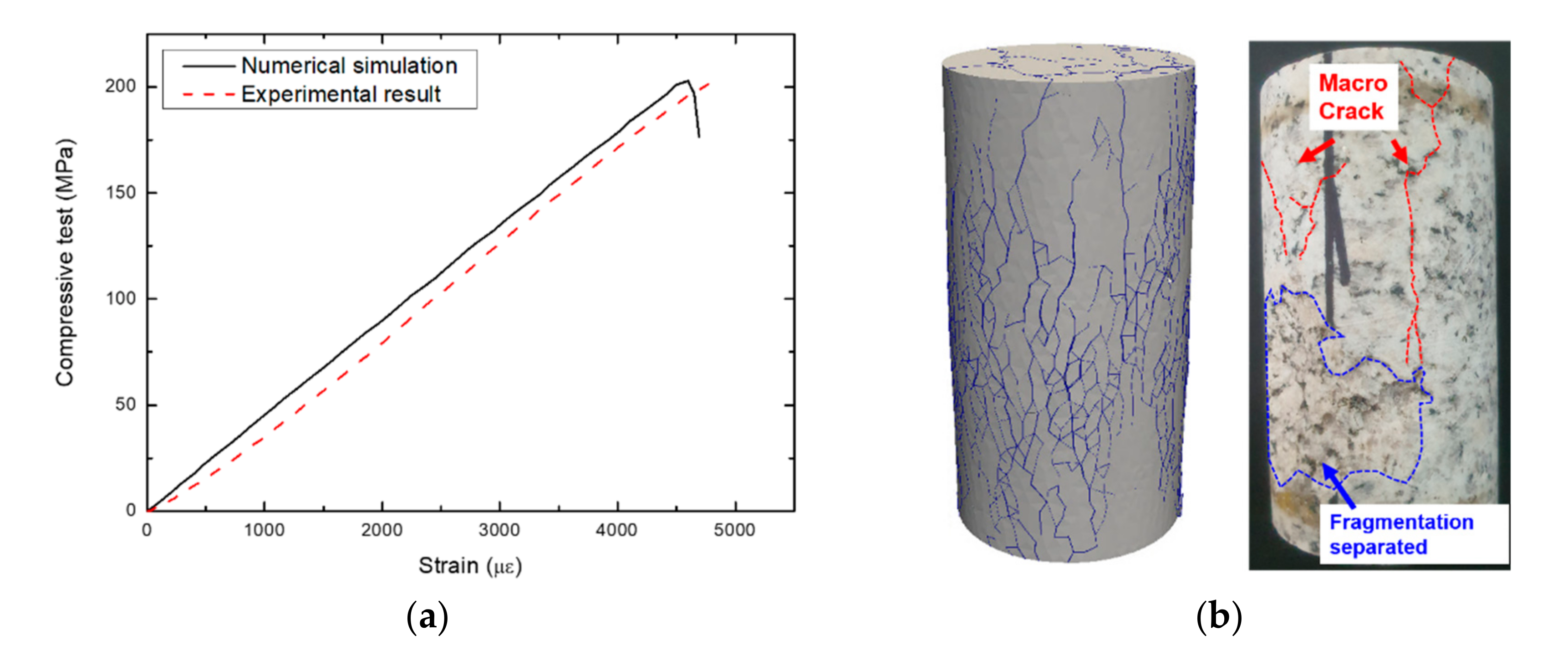
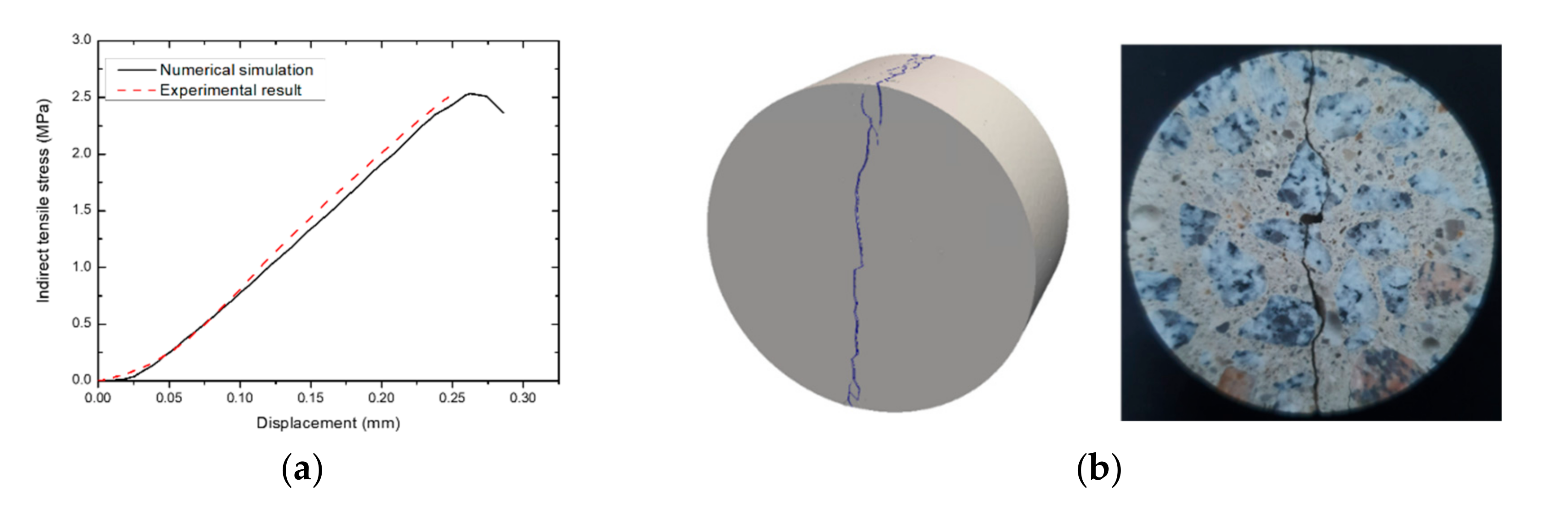
3. Calibration of the Combined Finite-Discrete Element Method by Modeling UCS and BTS

An appropriate determination of the model parameters is essential for accurate simulation of the shearing process in the C-R joint using FDEM. In this section, the failure processes in the UCS and BTS tests, which are frequently performed for acquiring mechanical properties of rock-like materials (i.e., rocks and concrete) are simulated using the 3D FDEM. The numerical simulation results are compared with experimental data to calibrate input parameters in the 3D FDEM. Figure 4 shows the 3D FDEM models for UCS and BTS tests. The calibration works are performed for a granite specimen and concrete specimen with nominal UCS = 35 MPa (hereafter, 35 MPa-concrete). The UCS and BTS test models are discretized around 1.5 mm of the tetrahedral element where the element size is sufficient to exclude the mesh sensitivity effect for the specimen size [47]. The experimentally obtained physical and mechanical properties of the granite and concrete specimens are summarized in Table 1. The input elastic parameters for the 3D FDEM models for granite and concrete were taken from the values in Table 1. Considering the literature [47], the normal contact penalty (Pn) and cohesive penalty terms ( P o p e n , P t a n , P o v e r l a p ) of the granite, concrete, and steel plates are assumed to be P n = 10 E , P o p e n = 100 E ,   P t a n = 100 E , and P o v e r l a p = 1000 E where E indicates the Young’s modulus of either rock (Erock) or concrete (Econc). The granite model or 35 MPa concrete model was placed between the top and bottom rigid loading plates with a slow velocity of 0.01 m / s [47] along with a critical damping scheme to approximately achieve a quasi-static loading condition [47,48,49,50].
Figure 5 and Figure 6 shows the comparison of the FDEM simulation and experiment during the UCS tests of the granite and the concrete, respectively. Figure 5a and Figure 6a present the plot of axial stress versus axial strain, and Figure 5b and Figure 6b indicate the final fracture pattern between numerical simulation and experiment test. The FDEM simulation result of the UCS test shown in Figure 5 and Figure 6 presents good agreement with the experiment result. Meanwhile, Figure 7 and Figure 8 show the comparison of the FDEM simulation and experiment during the BTS test of granite. In Figure 7a and Figure 8a, the plot of indirect tensile stress versus axial displacement is presented. Whereas in Figure 7b and Figure 8b, the final fracture pattern between numerical simulation and experiment test is on display. The FDEM simulation results of the BTS test shown in Figure 7 and Figure 8 are in agreement with the experiment results. Through the aforementioned calibration procedure of granite and 35 MPa concrete against the UCS and BTS tests, the calibrated input parameters for FDEM simulation of the direct shear test of the rough concrete–rock joint under shearing in the next section are summarized in Table 2 and Table 3.

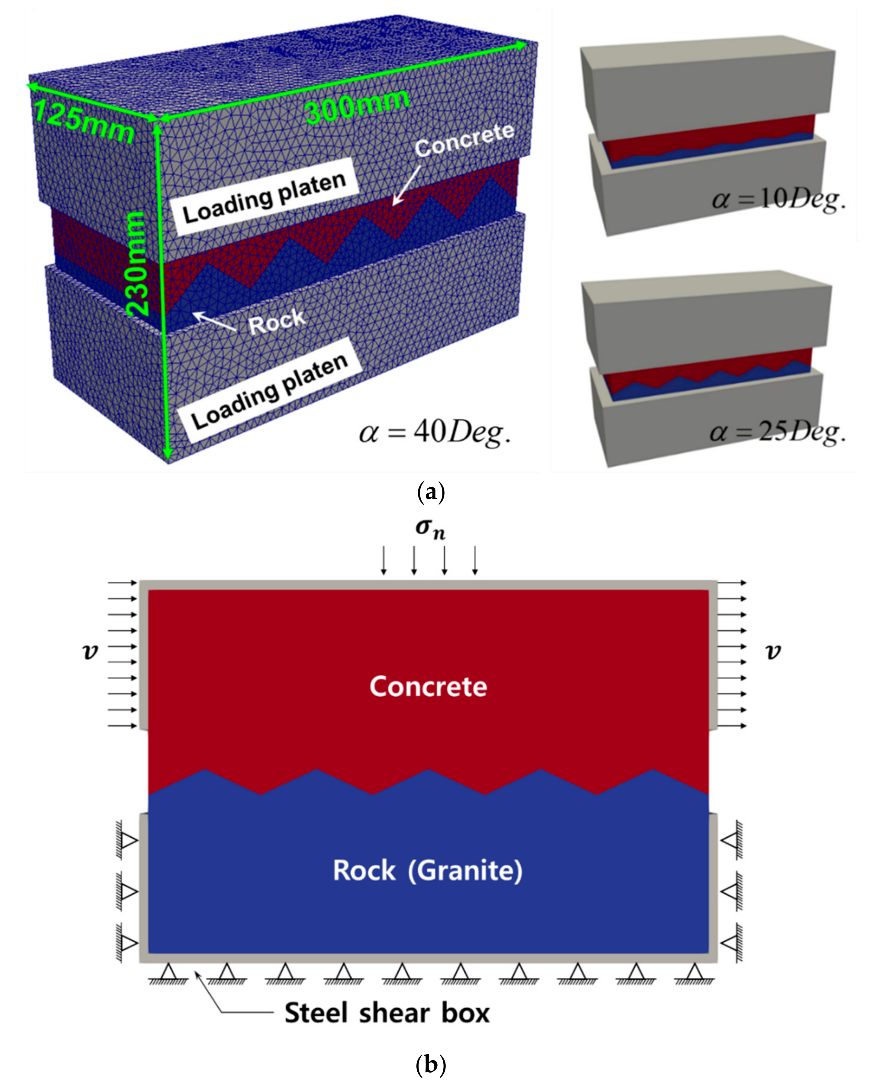
4. 3D FDEM Modeling of Rough Concrete–Rock Joint Failure in a Direct Shear Test

4.1. Modelling Procedure
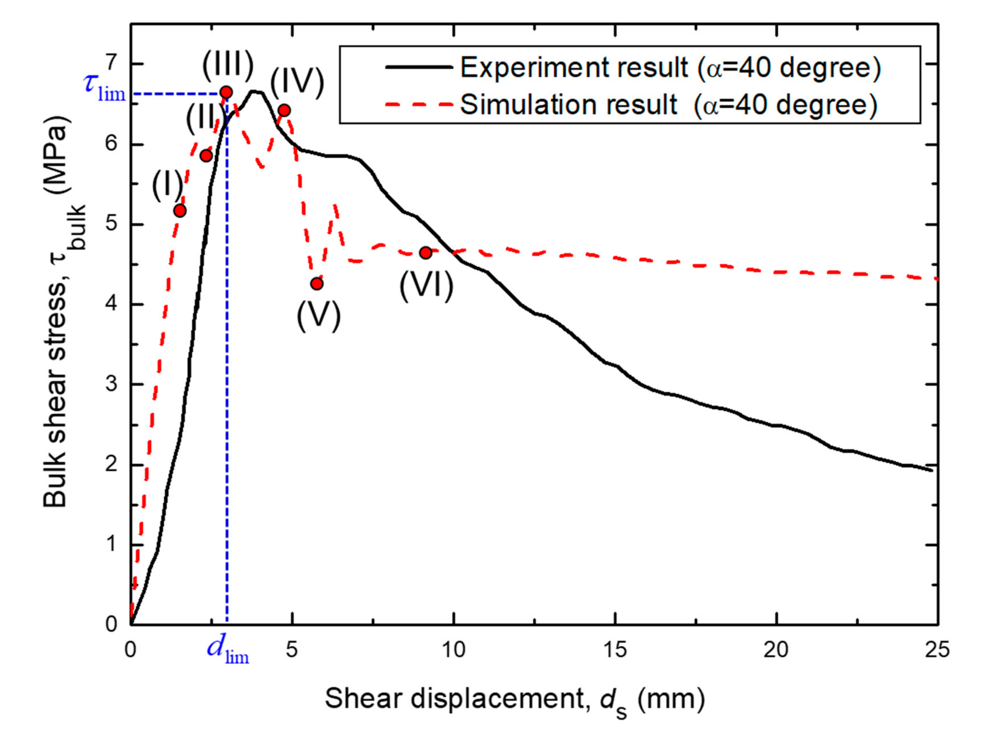
In this section, the 3D FDEM was employed to model the asperity dilatation, sliding, and degradation during the direct shear test of a rough C-R joint. As shown in Figure 9a, the 3D FDEM model has been generated and originally adopted as the direct shear test specimen. To compare the numerical simulation result with the direct shear test result, a simulation model was generated as an equivalent dimension on the experimental specimen. To consider the effect of asperity roughness of the C-R joint, we prepared three direct shear test models having the asperity angles of α = 40, 25, and 10 degrees (see Figure 9a). Note that the asperity angle is defined as the angle from the specimen base to the inclined plane. There is no suggested method or standards for the direct shear test of the C-R joint. The size of the direct shear test specimen was determined by considering the International Society for Rock Mechanics and Rock Engineering (ISRM) suggested method for the direct shear test of rock, which is presented in this literature [56]. Based on the ISRM suggested method, the test plane of the rock specimen should be exceeded by 10 times the maximum of the asperity height. In this study, we determined the asperity height between 5 and 25 mm, and the specimen width, length, and height were determined as 125 mm, 300 mm, and 230 mm, respectively. The FDEM model consists of discrete 35 MPa concrete and granite blocks. Both the concrete and granite blocks have a saw-tooth shape at the one end of each block. Along the saw-tooth shaped ends, the two blocks are placed in a way that each end perfectly matches to form the C-R joint. To apply normal and shear loadings to the blocks with the rock–concrete joint, we considered two half-boxes (hereafter called loading platens) partially covering the concrete and granite blocks (Figure 9b).
To provide a better understanding of the mechanical behavior of the C-R joint under self-weight loading, only a direct shearing test under CNL condition is considered here. The CNS conditions employed in most of the previous research [27,28,29] for describing C-R joints were not considered because the main interest of this paper is in the joint between the foundation and gravity anchorage in which the normal stress of the rock joint is expected to remain constant during shear deformation. In such cases, it is recommended to adopt the direct shear test with a CNL [57].
In the 3D FDEM simulation, normal confinement stress σn was applied to the top surface of the top loading platen (Figure 9b), while the bottom loading platen was kept in space to model the CNL condition. Then, the FDEM simulation continued until the static stress equilibrium was achieved in the C-R joint specimen. Note that the local damping scheme using a damping coefficient = 0.8 (coupled with mass scaling) [58] was utilized to accelerate the convergence rate to a static stress state. The cases of σn = 1.0, 2.0, and 3 MPa were considered. After this, the top loading plate was moved along the shear directions (i.e., horizontal direction in Figure 9b) with a constant velocity v = 0.01 m/s, while the bottom loading plate was fixed in space. Accordingly, shearing the discrete concrete–rock blocks under the CNL condition can be realized along the saw-tooth shape joint. It is worth mentioning that the damping scheme was switched from the local damping scheme (with mass scaling) to the critical damping scheme [36] at this stage to achieve the quasi-static loading condition. Otherwise, unrealistic spurious fracturing occurs due to unrealistic stress pile-up near the loading region. The material properties of concrete and granite blocks are set to the calibrated parameters in the previous section (Table 2 and Table 3).

4.2. Results

First, we present the results for case of the asperity angle α = 40 degrees. Figure 10 presents the shear stress–shear displacement curve obtained during our direct shear test simulation. Note that the shear displacement ds was defined by the horizontal displacement of the top-loading platen while the bulk shear stress τbulk was computed by dividing the horizontal contact force of the top-loading platen as an area (i.e., Area = Specimen width × Specimen length). Figure 11 shows the macroscopic crack propagation (i.e., CE6s with D =1 in Equation (3)) by white color (first column in Figure 11) and the maximum principal stress distribution (PS1) and minimum principal stress distribution (PS3) at different stages of the simulation. The tension stress is positive in PS1 and PS3. At the onset of the direct shear test, the constant σn was initially applied in the vicinity of the C-R joint as the boundary condition (i.e., CNL condition). When ds starts to increase, the concrete asperity sliding along the inclined C-R asperity surface and simultaneously surface friction is applied to the contact area of C-R joint surfaces, as shown in Figure 11a-I. In this stage, the tensile stress is induced near the contact asperity, as illustrated in Figure 11b-I. As these tensile stresses reached the tensile strength of CE6 in the vicinity of the asperity, the tensile crack was first initiated and propagated in a perpendicular direction to the contact area (Figure 11a-II). As shown as Figure 11a-IV, with the minor increase in ds, the existing tensile crack was continuously propagated in a perpendicular direction to the contact area, while a new tensile crack was created by the tensile stress reaching the strength in the vicinity of the asperity at different locations. The accumulation of damage induced by the continuous tensile and shear crack propagation significantly reduced the ability of asperity resistance by the further increase in the ds. As the tensile crack extends into the bases of the asperity (Figure 11a-V), the asperity is completely separated from their bases. Meanwhile, during the single asperity fracturing, other asperities were also fractured by the same fracturing process (see Figure 11III–V). When all of the asperities are completely separated from their bases as shown in Figure 11b-VI (marked as the yellow line), the overall behavior of the vicinity of the C-R joint behaves as a smooth surface. Figure 10 reflects the above-mentioned shear failure behavior of the C-R joint in terms of the bulk shear stress–shear displacement curve. Initially, the bulk shear stress increased linearly with the shear displacement (Figure 10-I), which was caused by dilation along the normal direction of the C-R joint. The dilatation was induced by sliding the C-R joint along the inclined surface and the dilatation effect of the friction force between the C-R joint by increasing normal forces to the friction area. When the tensile crack is initiated, the τbulk is slightly decreased with the ds increment (Figure 10-II). In this stage, the PS3 distribution changed along the tensile crack because the single asperity behaved as sliding along the crack surface rather than dilatation as the ds increases. However, the τbulk still increased due to local normal stress increment in the other asperities (see Figure 10II–III), until the τbulk approached the shear resistance limit, τlim (Figure 10-III). In this stage, the fluctuation of τbulk is presented because during the single asperity fracture, the other asperities are in various fracturing processes (i.e., crack initiation and propagation). After further ds, the accumulation of damage induced by continuous tensile crack propagation significantly reduced the ability of asperity resistance. This stage corresponds to the transition from the post-peak reduction of τbulk to residual stress regime (Figure 10-IV–V). As the tensile crack extended into the bases of the asperity (Figure 10-VI), the asperity was completely separated from their bases and behaved as a smooth surface passing through the base of the concrete asperity. In this condition, the effect of the roughness of the concrete–rock joint became almost negligible, and the main factor for shear resistance was changed to sliding, which was subjected to normal loading. In Figure 10, before the shear softening, the numerical simulation presented good agreement with the experiment result in the τlim and the dlim. However, in the regime of residual shear resistance, the shear resistance behavior was different from the laboratory direct shear test result. In the regime of the residual resistance, the numerical simulation presented as τbulk remained almost in constant residual shear stress, but the experiment showed a continuous decrease after the peak τbulk. Comparing to the resultant fracture pattern between the simulation and experiment result as shown in Figure 12, the smooth surface was generated in both cases. However, additional damages (i.e., cracks and fragmentation) were found in the experiments, as shown in Figure 12b.

5. Discussion

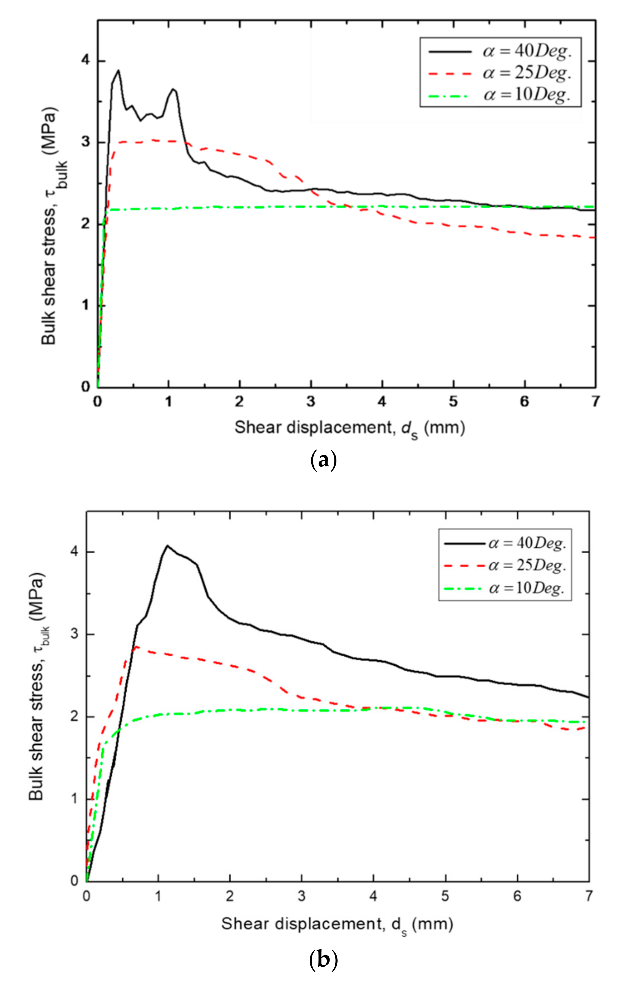
5.1. Direct Shearing of Concrete–Rock Joint with Different Asperity Roughness

The direct shear test of concrete–rock joints with various roughness and regular triangular asperity was simulated using the 3D FDEM to investigate the effect of joint roughness on the shear failure process. Figure 13 and Figure 14 compare the three concrete–rock joint models with the asperity angles of α = 10 and 25 degrees in terms of the distributions of the maximum principal stress (PS1) and the macroscopic cracks. The case of α = 40 degrees was already presented in Figure 11-VI. Similarly to Figure 10, the τbulkds curves for the three asperity angles α = 10, 25, and 40 degrees in terms of σn = 2.0 MPa are compared in Figure 15. As already explained using Figure 11-VI for the case of rougher asperity (α = 40 degrees), the main fracture mechanism in overall shear resistance was joint asperity degradation, which was induced by tensile fracturing within the intact asperity. As can be seen from Figure 13 and Figure 14 for the relatively smoother asperity (α = 10 and 25 degrees), sliding was the main mechanism in the overall shear resistance. Since the smoother single asperity was more free from the bending moment, which more easily induced the tensile crack than the rough single asperity, the only factor of the shear resistance in the smooth asperity was the friction between the top (concrete) and bottom (rock) asperity. Figure 15a indicates that the relatively rougher asperity (α = 40 degrees) shows clear shear softening behavior (transition from peak bulk shear stress to reduction) due to the joint asperity degradation. With the decrease of the asperity angle α, the shear softening behavior due to the joint asperity degradation became less obvious and in the case of α = 10 degrees only showed constant τbulk, i.e., a residual stress state immediately after the initial elastic behavior. Compared to the development of shear resistance between the simulation and experiment result in terms of the τbulkds curves as shown in Figure 15a,b, the overall development of shear resistance presents similar behaviors at each case of the α. However, the fluctuation of the τbulk is observed around the peak bulk shear stress in the numerical simulation, while the τbulk shows the stress-drop after the peak bulk shear stress in the experiment.
To interpret the obtained results more clearly, the FDEM simulation results for various values of α (α = 10, 25 and 40 degrees) and σn (i.e., σn = 1.0, 2.0 and 3.0 MPa) were fitted using a linear fitting line based on the M-C shear failure criteria as shown in Figure 16. To avoid confusion caused by notation between the microscopic cohesion and internal friction angle, which is summarized in Table 2, and the parameters of the M-C shear failure criteria, the M-C parameter is presented as the bulk cohesion (cbulk) and bulk internal friction angle ( ϕ bulk). In addition, the cbulk and ϕ bulk reflect the overall shear resistance in the vicinity of the C-R joint, unlike the microscopic cohesion and internal friction angle represented in a single material. In this figure, the shear strength for each case was computed as the peak value of each of the τbulkds curves for different conditions. In this M-C shear failure criteria, the bulk cohesion (cbulk) is considered as zero because of an unbounded condition between the concrete and rock surface. In addition, the bulk internal friction angle ( ϕ bulk) was determined by calculating the slope of each linear fitting line. The figure clearly shows that the increase in normal stress increments based on the M-C theory and the internal friction angle ( ϕ bulk) also increased with asperity angle increments. These simulation results follow Patton’s theoretical model [10], which represents the effect of joint roughness as the increment of the internal friction angle,   ϕ , (e.g., τ b u l k = t a n ϕ + ϕ ) when the asperity angle, i.e., joint roughness, increases. Ultimately, such results validate the applicability of the 3D FDEM to this class of problem involving joint surface interaction.

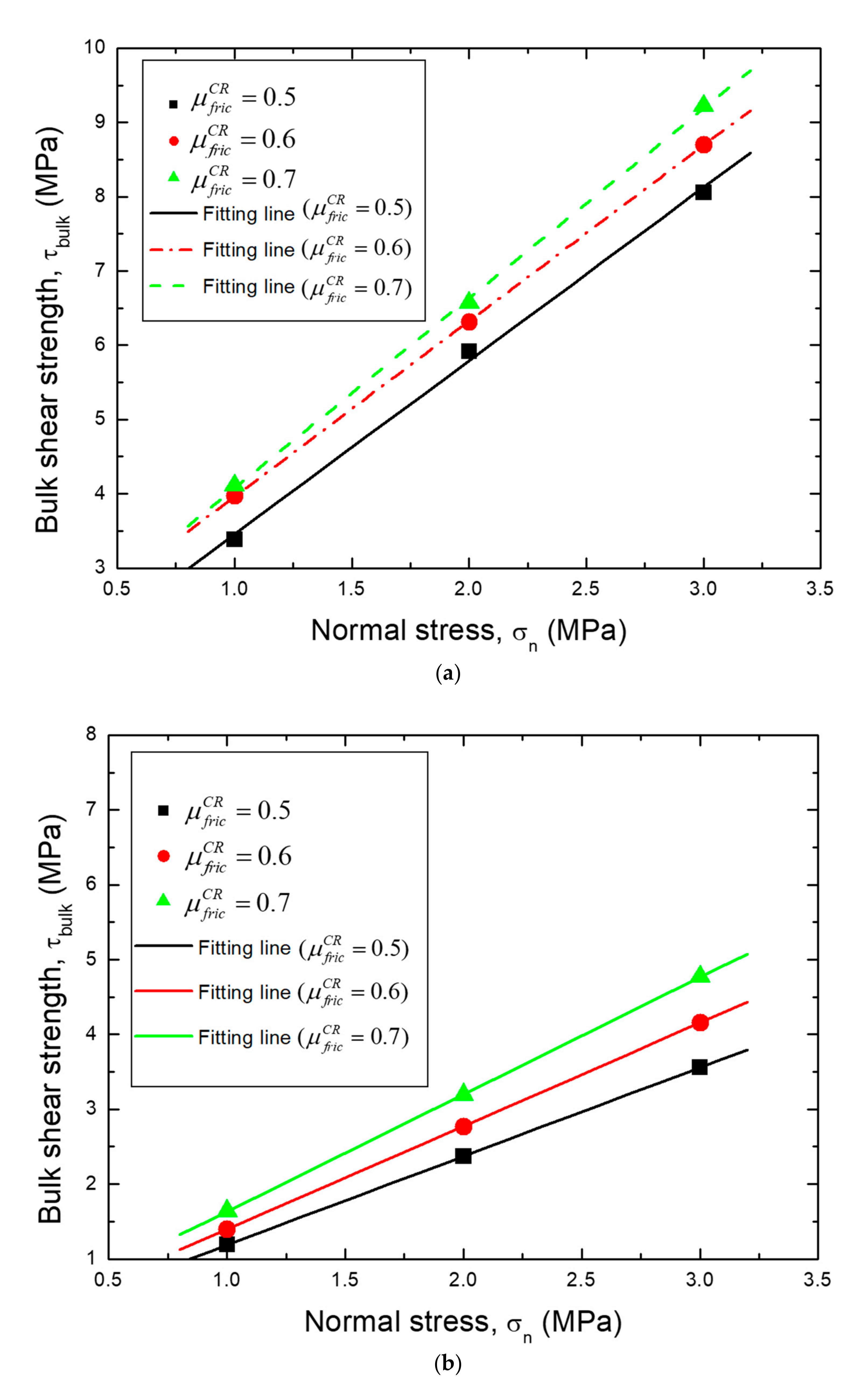
5.2. Effect of Fiction Coefficient on Direct Shearing of Concrete–Rock Joint

The effect of the friction coefficient on the direct shearing of the rough C-R joint was examined by performing a direct shear test on the C-R joint with a different friction coefficient. In an FDEM simulation, the friction coefficient has been applied for calculating shear forces on the contacting macro crack surface in a single material and contacting surface between different materials. The detailed description for the calculation of the contact and shear force can be found in the literature [49,50]. For calculating the shear forces on contacting surfaces, several FDEM numerical simulations [39,47,50], including this study, have applied the constant friction coefficient between rock and rock as 0.5–0.6 when a macroscopic crack surface is newly generated. In addition, the constant friction coefficient between the rock and loading platen is determined as 0.1. Using these values, they acquire quite similar results in essential quasi-static test simulations such as UCS and BTS. However, the friction coefficient between different materials (e.g., C-R joint) should carefully be considered, especially in the direct shear test. The friction force, varied by friction coefficient, may present a different fracture pattern and bulk shear strength in the vicinity of the C-R joint. Moreover, the friction coefficient may affect the internal friction angle ( ϕ bulk) due to how the basic friction angle [6,10], which was acquired by direct testing a flat joint, determines the internal friction angle in the rock joint as a similar parameter with a friction coefficient in the FDEM. In this sense, the inspection of the effect of the friction coefficient on the C-R joint should carefully be considered.
In this study, the friction coefficient, expressed as μ fric CR in Table 3, varied between 0.5, 0.6, and 0.7. Under different friction coefficients, the simulation of a direct shear test was performed on the C-R joint with α = 10 and 40 degrees of saw-tooth asperity under various values of σn (i.e., σn = 1.0, 2.0, and 3.0 MPa).
As can be seen in the Figure 17, the τbulk is presented as a function of σn in terms of different μ fric CR (i.e., μ f r i c C R = 0.5, 0.6, and 0.7) and α (i.e., α = 10 and 40 degrees). Figure 17 shows that the bulk shear strength increases with μ f r i c C R increments in both α = 10 and 40 degrees. In Figure 17a,b, the ϕ bulk may be more dependent on the μ fric CR in the α = 10 than 40 degrees because the ϕ bulk was almost constant with the α = 40 degrees, while the ϕ bulk increases with the friction coefficient increment in the α = 10 degrees. Sliding is the main mechanism in the smooth joint (i.e., α = 10) and the μ fric CR directly increased the friction as well as the bulk shear strength at the concrete–rock joint. The asperity degradation occurs in the rough joint (i.e., α = 40) in the vicinity of the concrete asperity base. The friction applied at the macroscopic crack in the concrete part and ϕ bulk may be independent with the variation of μ fric CR .

6. Conclusions

In this study, a GPGPU-parallelized FDEM was applied to model the shear failure process of a rough concrete–rock joint in direct shear tests under constant normal loading conditions. Before simulating the direct shear test, the combined finite-discrete element method was calibrated by simulating the concrete and rock fracture process in the UCS and BTS tests and was compared with the experimental results. Then, the direct shear test of the concrete–rock joint was modeled using the combined finite-discrete element method to investigate the shear resistance process of a concrete–rock joint. We focused on the asperity dilatation, sliding, and degradation in terms of various asperity roughness under different constant normal loading (CNL) conditions. The effect of the joint roughness and friction coefficient between the concrete and rock interface on the behavior of the shear resistance was also discussed. In this study, the following conclusions can be drawn:
(1)
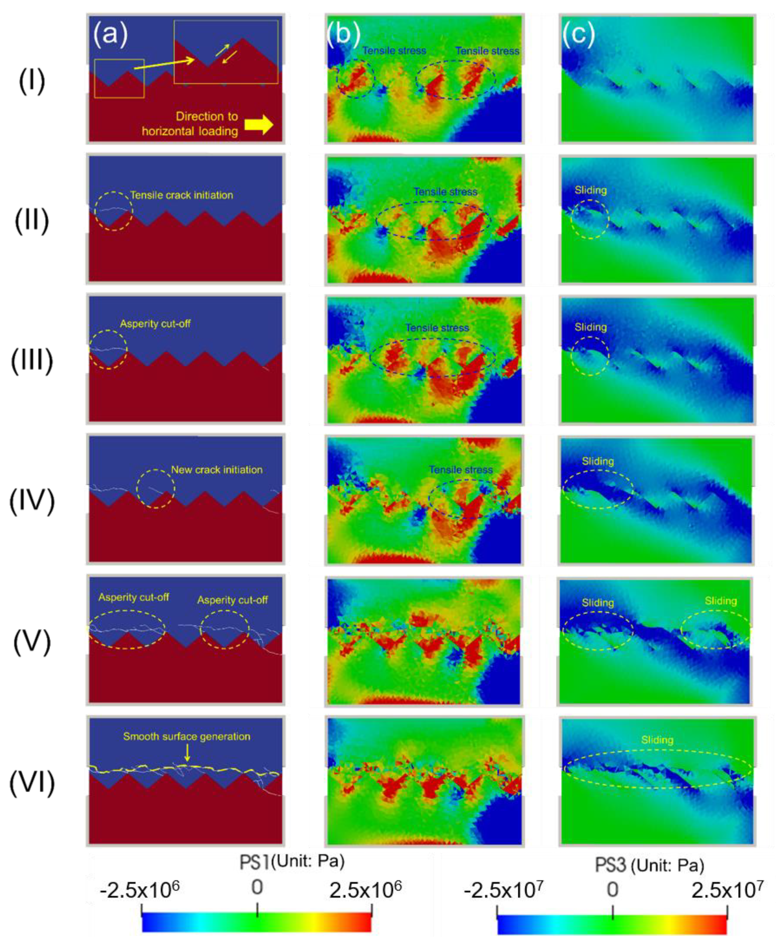
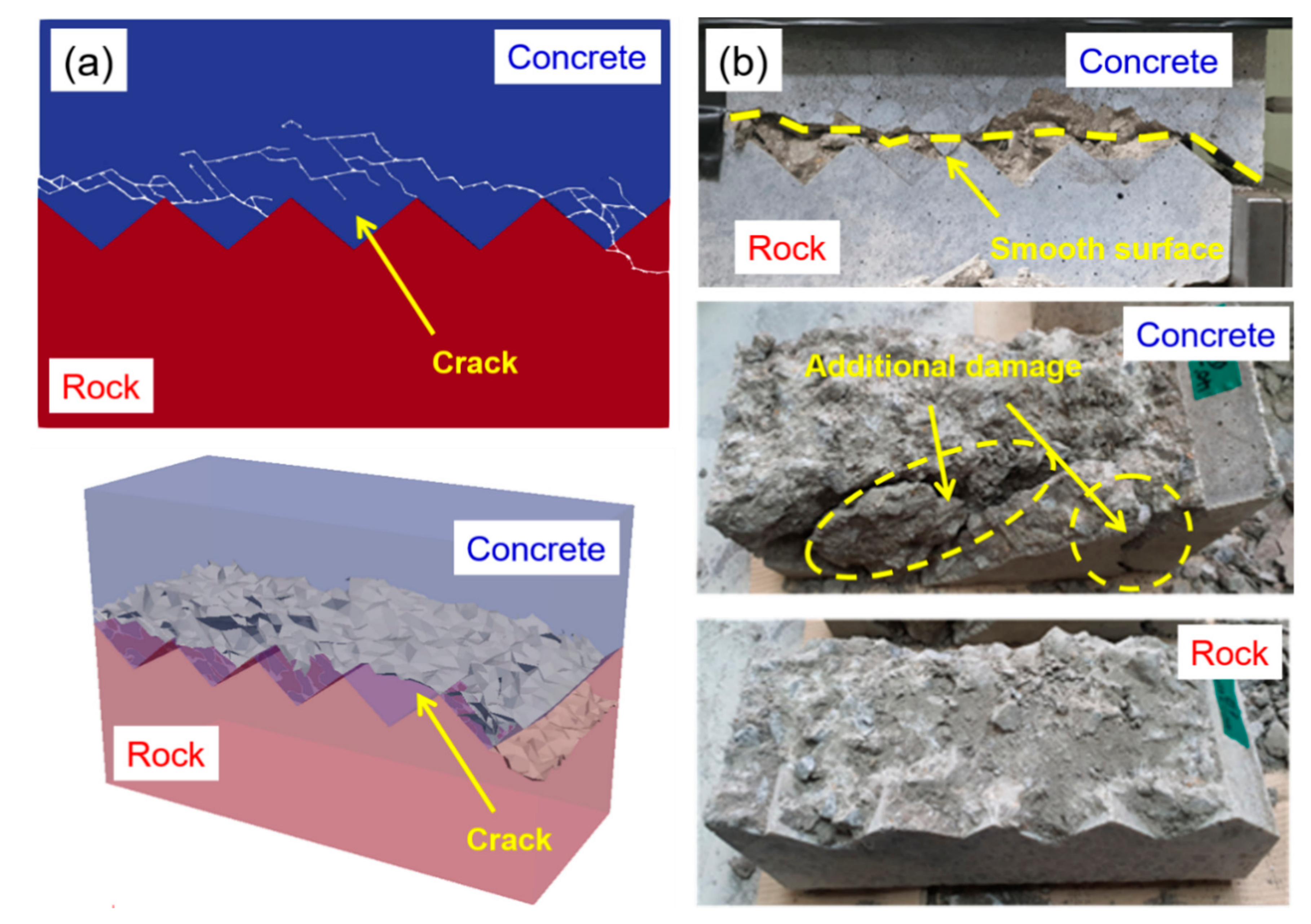
The GPGPU-parallelized FDEM reproduced the asperity dilatation, sliding, and degradation on the direct shear test of the concrete–rock joint with rough saw-tooth triangular asperity. Compared with laboratory observation, the simulation result presented a good agreement on the bulk shear stress–horizontal displacement curve before the regime of residual shear resistance. However, the laboratory test results presented a continuous decrease of bulk shear stress unlike the numerical simulation result, which showed constant residual stress after shear softening. In this study, we concluded that the additional damages found in the experiment results induced a continuous stress drop and presented different behaviors in the numerical simulation in the regime of the constant residual stress statement.
(2)
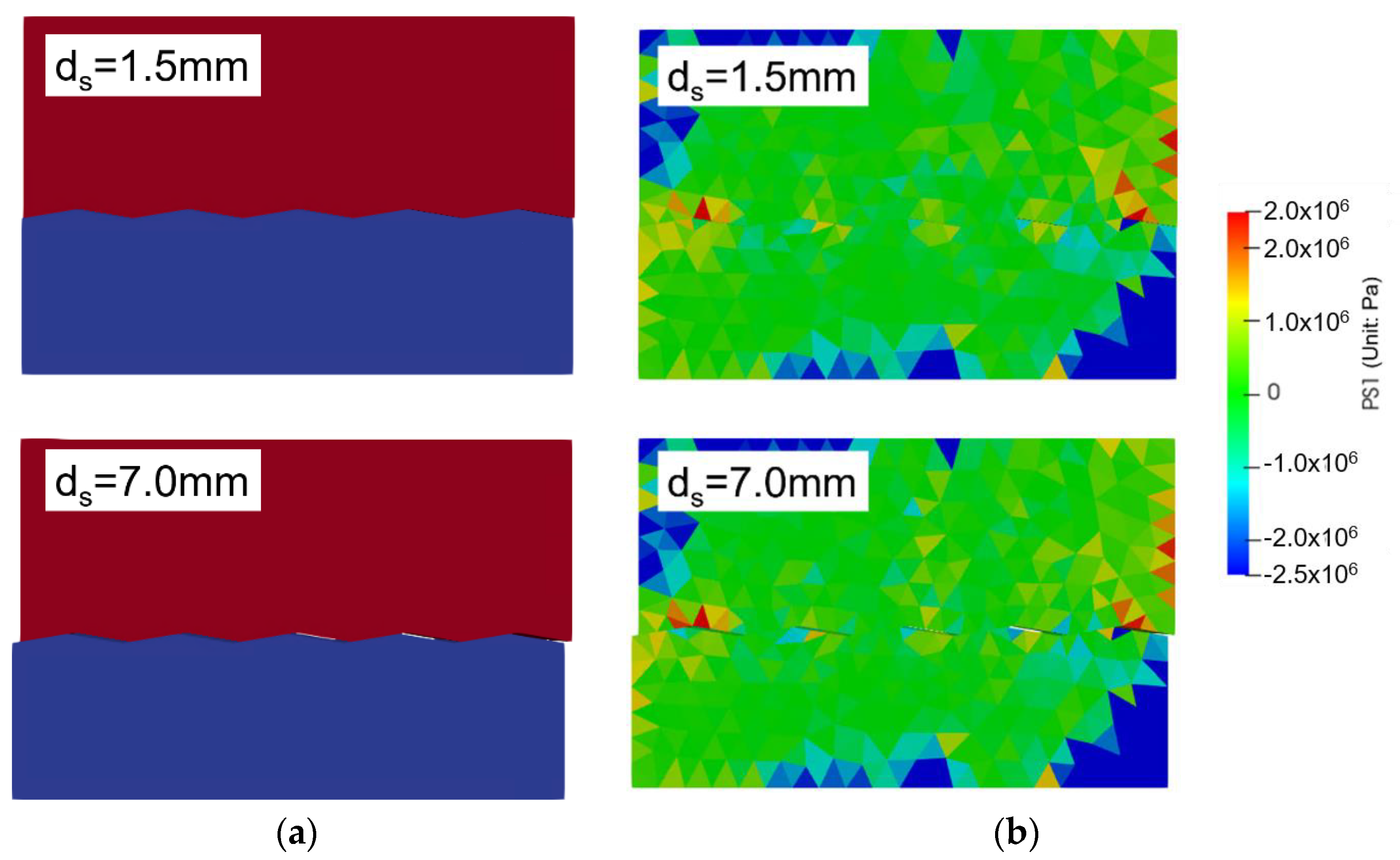
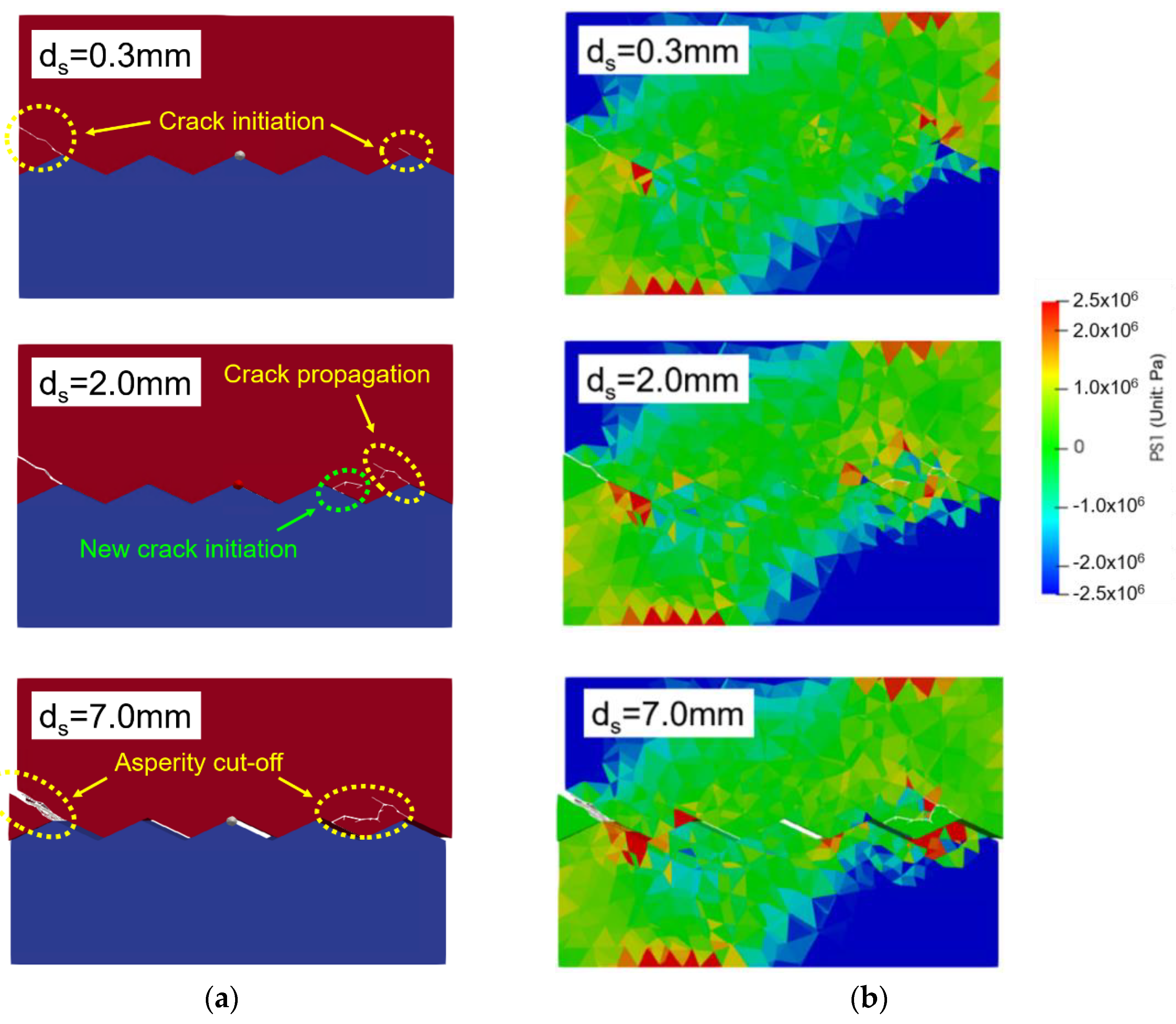
The roughness of asperities in the concrete–rock joint affects the overall joint shear resistance, where the main fracture mechanism is asperity sliding in the smooth asperity and asperity degradation in the rough asperity. The smoother single asperity is freer from the bending moment, which was easy to induce in the tensile crack in concrete asperity base, than the rough single asperity. The only factor of the shear resistance in the smooth asperity is the friction between the concrete and rock joint interface. The effect of the increment of asperity roughness affects the shear strength increment and causes the asperity degradation, which presents the shear softening behavior after the peak bulk shear stress, while the smooth asperity roughness presents the residual stress statement immediately after the initial elastic behavior. In addition, when the direct shear test results are presented as Mohr–Coulomb criterion, the bulk internal friction angle was clearly increased with an increasing asperity angle. In this study, the effect of asperity roughness on the bulk internal friction angle follows the Patton’s theoretical model.
(3)
The friction coefficient is an important parameter for simulating the direct shearing of the concrete–rock joint. Especially, the friction coefficient was more effective on the internal friction angle in terms of the smooth joint than the rough joint. The asperity degradation was the main mechanism in the rough joint, the concrete asperity base was fractured, and the friction was applied at the macroscopic crack surface in the concrete asperity base. Thus, the internal friction angle in the vicinity of the rough concrete–rock joint may be independent of the friction coefficient between the rock and concrete. However, in the smooth joint, the main mechanism of shear resistance was sliding without fracturing, and the different friction coefficient was directly reflected to the friction force as well as the internal friction angle.

Author Contributions

Conceptualization, Y.K., M.C. and S.C.; methodology, G.M., D.F., S.O., Y.K., H.L., M.C. and S.C.; investigation, G.M., D.F., S.O. and S.C.; writing—original draft preparation, G.M., D.F. and S.C.; writing—review and editing, G.M., D.F., H.L. and S.C.; visualization, G.M., S.O., G.K. and S.C.; supervision, M.C. and S.C.; project administration, Y.K., M.C. and S.C. All authors have read and agreed to the published version of the manuscript.

Funding

This research was supported by a grant (20SCIP-B119947-05) from Construction Technology Research Program funded by Ministry of Land, Infrastructure and Transport of Korean government.

Acknowledgments

The authors would like to thank the Writing Center at Jeonbuk National University for its skilled proofreading service.

Conflicts of Interest

The authors declare no conflict of interest.

References

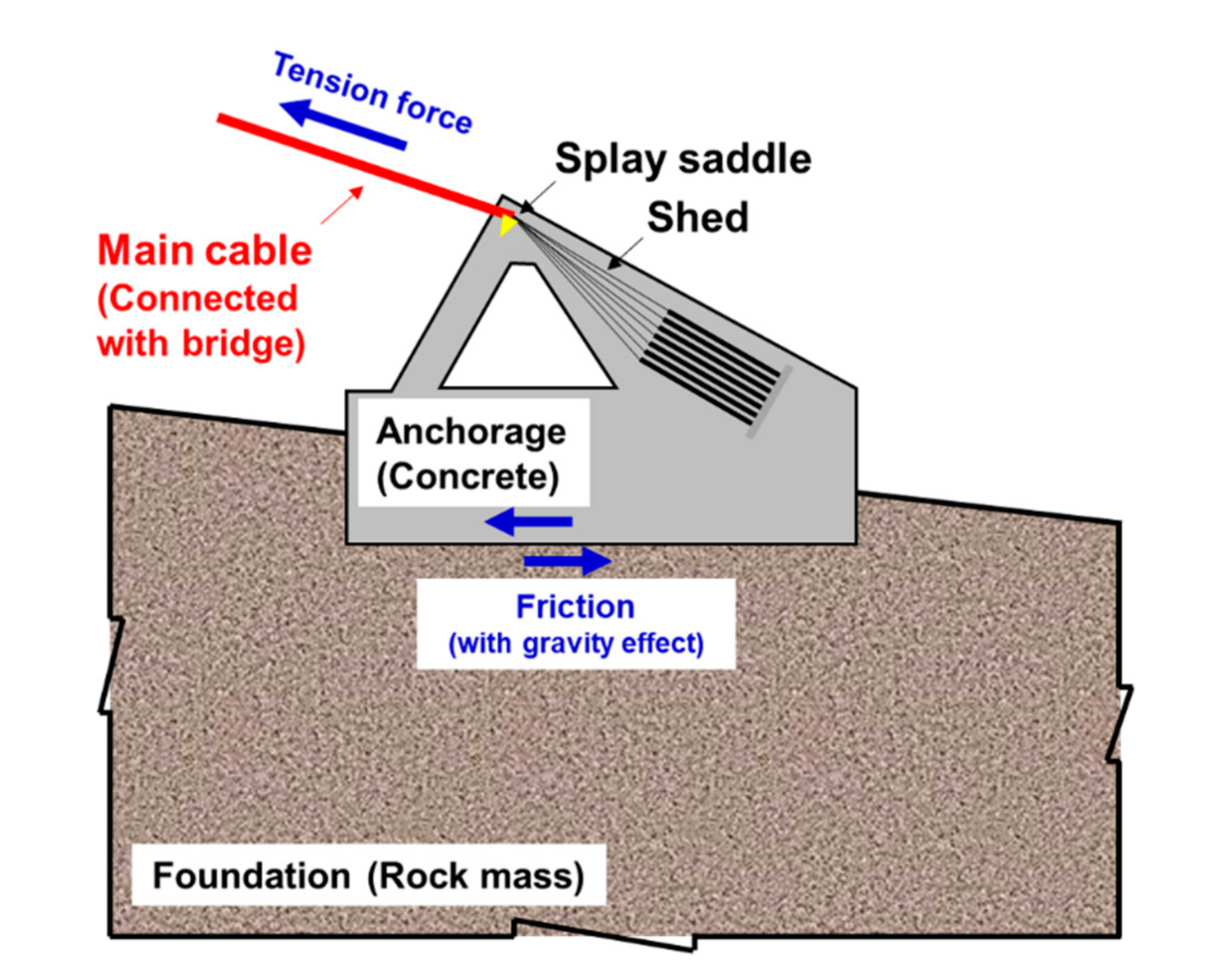
  1. Han, Y.; Liu, X.; Wei, N.; Li, D.; Deng, Z.; Wu, X.; Liu, D. A Comprehensive Review of the Mechanical Behavior of Suspension Bridge Tunnel-Type Anchorage. Adv. Mater. Sci. Eng. 2019, 2019, 1–19. [Google Scholar] [CrossRef] [Green Version]
  2. AASHTO, LFRD. Standard Specifications for Highway Bridges, 17th ed.; American Association of State Highway and Transportation: Washington, DC, USA, 2002. [Google Scholar]
  3. American Association of State Highway Transportation. Highway Safety Manual; Officials; AASHTO: Washington, DC, USA, 2010; Volume 1. [Google Scholar]
  4. Bond, A.; Harris, A. Decoding Eurocode 7; CRC Press: London, UK, 2006. [Google Scholar]
  5. Japan Road Association. Design Specifications of Highway Bridges, Part V Seismic Design; Maruzen: Tokyo, Japan, 2002. [Google Scholar]
  6. Korea Road and Transportation Association. Korea Bridge Design Code; Ministry of Land, Transport and Maritime Affairs: Seoul, Korea, 2012. [Google Scholar]
  7. Barton, N.; Choubey, V. The shear strength of rock joints in theory and practice. Rock Mech. Rock Eng. 1977, 10, 1–54. [Google Scholar] [CrossRef]
  8. Jaeger, J.C. Friction of Rocks and Stability of Rock Slopes. Géotechnique 1971, 21, 97–134. [Google Scholar] [CrossRef]
  9. Ladanyi, B.; Archambault, G. Simulation of shear behavior of a jointed rock mass. In Proceedings of the 11th US Symposium on Rock Mechanics (USRMS), Berkeley, CA, USA, 16–19 June 1969. [Google Scholar]
  10. Patton, F.D. Multiple modes of shear failure in rock. In Proceedings of the 1st ISRM Congress, Lisbon, Portugal, 25 September–1 October 1966. [Google Scholar]
  11. Lam, T.S.K.; Johnston, I.W. Shear Behavior of Regular Triangular Concrete/Rock Joints—Evaluation. J. Geotech. Eng. 1989, 115, 728–740. [Google Scholar] [CrossRef]
  12. Johnston, I.W.; Lam, T.S.K. Shear Behavior of Regular Triangular Concrete/Rock Joints—Analysis. J. Geotech. Eng. 1989, 115, 711–727. [Google Scholar] [CrossRef]
  13. Barton, N. Shear strength criteria for rock, rock joints, rockfill and rock masses: Problems and some solutions. J. Rock Mech. Geotech. Eng. 2013, 5, 249–261. [Google Scholar] [CrossRef] [Green Version]
  14. Amadei, B.; Saeb, S. Constitutive models of rock joints. In Proceedings of the International Symposium on Rock Joints, Loen, Norway, 4–6 June 1990; pp. 581–594. [Google Scholar]
  15. Lee, H.; Park, Y.; Cho, T.; You, K. Influence of asperity degradation on the mechanical behavior of rough rock joints under cyclic shear loading. Int. J. Rock Mech. Min. Sci. 2001, 38, 967–980. [Google Scholar] [CrossRef]
  16. Hossaini, K.A.; Babanouri, N.; Nasab, S.K. The influence of asperity deformability on the mechanical behavior of rock joints. Int. J. Rock Mech. Min. Sci. 2014, 70, 154–161. [Google Scholar] [CrossRef]
  17. Plesha, M.E. Constitutive models for rock discontinuities with dilatancy and surface degradation. Int. J. Numer. Anal. Methods Gíomích. 1987, 11, 345–362. [Google Scholar] [CrossRef]
  18. Souley, M.; Homand, F.; Amadei, B. An extension to the Saeb and Amadei constitutive model for rock joints to include cyclic loading paths. Int. J. Rock Mech. Min. Sci. Geomech. Abstr. 1995, 32, 101–109. [Google Scholar] [CrossRef]
  19. Maksimović, M. The shear strength components of a rough rock joint. Int. J. Rock Mech. Min. Sci. Geomech. Abstr. 1996, 33, 769–783. [Google Scholar] [CrossRef]
  20. Haque, A.; Indraratna, B. Shear Behaviour of Rock Joints; CRC Press: Boca Raton, FL, USA, 2000. [Google Scholar]
  21. Olsson, R.; Barton, N. An improved model for hydromechanical coupling during shearing of rock joints. Int. J. Rock Mech. Min. Sci. 2001, 38, 317–329. [Google Scholar] [CrossRef]
  22. Serrano, A.; Olalla, C.; Galindo-Aires, R.Á. Micromechanical basis for shear strength of rock discontinuities. Int. J. Rock Mech. Min. Sci. 2014, 70, 33–46. [Google Scholar] [CrossRef] [Green Version]
  23. Indraratna, B.; Thirukumaran, S.; Brown, E.T.; Zhu, S.-P. Modelling the Shear Behaviour of Rock Joints with Asperity Damage Under Constant Normal Stiffness. Rock Mech. Rock Eng. 2014, 48, 179–195. [Google Scholar] [CrossRef]
  24. Hencher, S.R.; Richards, L.R. Assessing the Shear Strength of Rock Discontinuities at Laboratory and Field Scales. Rock Mech. Rock Eng. 2014, 48, 883–905. [Google Scholar] [CrossRef]
  25. Shrivastava, A.K.; Rao, K.S. Shear Behaviour of Rock Joints Under CNL and CNS Boundary Conditions. Geotech. Geol. Eng. 2015, 33, 1205–1220. [Google Scholar] [CrossRef]
  26. Bahaaddini, M.; Hagan, P.C.; Mitra, R.; Hebblewhite, B.K. Parametric Study of Smooth Joint Parameters on the Shear Behaviour of Rock Joints. Rock Mech. Rock Eng. 2014, 48, 923–940. [Google Scholar] [CrossRef]
  27. Kodikara, J.; Johnston, I. Shear behaviour of irregular triangular rock-concrete joints. Int. J. Rock Mech. Min. Sci. Geoomech. Abstr. 1994, 31, 313–322. [Google Scholar] [CrossRef]
  28. Gu, X.F.; Seidel, J.P.; Haberfield, C.M. Direct Shear Test of Sandstone-Concrete Joints. Int. J. Geomech. 2003, 3, 21–33. [Google Scholar] [CrossRef]
  29. Saiang, D.; Malmgren, L.; Nordlund, E. Laboratory Tests on Shotcrete-Rock Joints in Direct Shear, Tension and Compression. Rock Mech. Rock Eng. 2005, 38, 275–297. [Google Scholar] [CrossRef]
  30. Seidel, J.P.; Haberfield, C.M. A theoretical model for rock joints subjected to constant normal stiffness direct shear. Int. J. Rock Mech. Min. Sci. 2002, 39, 539–553. [Google Scholar] [CrossRef]
  31. Haberfield, C.; Johnston, I. A mechanistically-based model for rough rock joints. Int. J. Rock Mech. Min. Sci. Geomech. Abstr. 1994, 31, 279–292. [Google Scholar] [CrossRef]
  32. Tian, H.M.; Chen, W.; Yang, D.S.; Yang, J.P. Experimental and Numerical Analysis of the Shear Behaviour of Cemented Concrete–Rock Joints. Rock Mech. Rock Eng. 2014, 48, 213–222. [Google Scholar] [CrossRef]
  33. Bahaaddini, M.; Sharrock, G.; Hebblewhite, B. Numerical direct shear tests to model the shear behaviour of rock joints. Comput. Geotech. 2013, 51, 101–115. [Google Scholar] [CrossRef]
  34. Park, J.-W.; Song, J.-J. Numerical simulation of a direct shear test on a rock joint using a bonded-particle model. Int. J. Rock Mech. Min. Sci. 2009, 46, 1315–1328. [Google Scholar] [CrossRef]
  35. Munjiza, A. Discrete Elements in Transient Dynamics of Fractured Media. Ph.D. Thesis, Swansea University, Swansea, UK, 1992. [Google Scholar]
  36. Munjiza, A.A. The Combined Finite-Discrete Element Method; John Wiley & Sons: Hoboken, NJ, USA, 2004. [Google Scholar]
  37. Munjiza, A.A.; Knight, E.E.; Rougier, E. Computational Mechanics of Discontinua; John Wiley & Sons: Hoboken, NJ, USA, 2011. [Google Scholar]
  38. Munjiza, A.; Knight, E.E.; Rougier, E. Large Strain Finite Element Method: A Practical Course; John Wiley & Sons: Hoboken, NJ, USA, 2015. [Google Scholar]
  39. Mahabadi, O.K.; Lisjak, A.; Munjiza, A.; Grasselli, G. Y-Geo: New Combined Finite-Discrete Element Numerical Code for Geomechanical Applications. Int. J. Geomech. 2012, 12, 676–688. [Google Scholar] [CrossRef]
  40. Yan, C.; Jiao, Y. A 2D fully coupled hydro-mechanical finite-discrete element model with real pore seepage for simulating the deformation and fracture of porous medium driven by fluid. Comput. Struct. 2018, 196, 311–326. [Google Scholar] [CrossRef]
  41. Yan, C.; Jiao, Y.-Y.; Zheng, H. A fully coupled three-dimensional hydro-mechanical finite discrete element approach with real porous seepage for simulating 3D hydraulic fracturing. Comput. Geotech. 2018, 96, 73–89. [Google Scholar] [CrossRef]
  42. Lisjak, A.; Mahabadi, O.; He, L.; Tatone, B.; Kaifosh, P.; Haque, S.; Grasselli, G. Acceleration of a 2D/3D finite-discrete element code for geomechanical simulations using General Purpose GPU computing. Comput. Geotech. 2018, 100, 84–96. [Google Scholar] [CrossRef]
  43. Rougier, E.; Bradley, C.R.; Broom, S.T.; Knight, E.E.; Munjiza, A.; Sussman, A.J.; Swift, R.P. The Combined Finite-Discrete Element Method Applied to the Study of Rock Fracturing Behavior in 3D; Los Alamos National Lab. (LANL): Los Alamos, NM, USA, 2011. [Google Scholar]
  44. An, H.; Liu, H.Y.; Han, H.; Zheng, X.; Wang, X. Hybrid finite—discrete element modelling of dynamic fracture and resultant fragment casting and muck-piling by rock blast. Comput. Geotech. 2017, 81, 322–345. [Google Scholar] [CrossRef]
  45. Liu, H.Y.; Kang, Y.M.; Lin, P. Hybrid finite—discrete element modeling of geomaterials fracture and fragment muck-piling. Int. J. Geotech. Eng. 2013, 9, 115–131. [Google Scholar] [CrossRef]
  46. Liu, H.Y.; Han, H.; An, H.M.; Shi, J.J. Hybrid finite-discrete element modelling of asperity degradation and gouge grinding during direct shearing of rough rock joints. Int. J. Coal Sci. Technol. 2016, 3, 295–310. [Google Scholar]
  47. Mohammadnejad, M.; Fukuda, D.; Liu, H.Y.; Dehkhoda, S.; Chan, A. GPGPU-parallelized 3D combined finite–discrete element modelling of rock fracture with adaptive contact activation approach. Comput. Part. Mech. 2019, 7, 849–867. [Google Scholar] [CrossRef]
  48. Mohammadnejad, M.; Dehkhoda, S.; Fukuda, D.; Liu, H.Y.; Chan, A. GPGPU-parallelised hybrid finite-discrete element modelling of rock chipping and fragmentation process in mechanical cutting. J. Rock Mech. Geotech. Eng. 2020, 12, 310–325. [Google Scholar] [CrossRef]
  49. Fukuda, D.; Mohammadnejad, M.; Liu, H.; Dehkhoda, S.; Chan, A.; Cho, S.; Min, G.; Han, H.; Kodama, J.; Fujii, Y. Development of a GPGPU-parallelized hybrid finite-discrete element method for modeling rock fracture. Int. J. Numer. Anal. Methods Geomech. 2019, 43, 1797–1824. [Google Scholar] [CrossRef]
  50. Fukuda, D.; Mohammadnejad, M.; Liu, H.-Y.; Zhang, Q.; Zhao, J.; Dehkhoda, S.; Chan, A.; Kodama, J.-I.; Fujii, Y. Development of a 3D Hybrid Finite-Discrete Element Simulator Based on GPGPU-Parallelized Computation for Modelling Rock Fracturing Under Quasi-Static and Dynamic Loading Conditions. Rock Mech. Rock Eng. 2019, 53, 1079–1112. [Google Scholar]
  51. Han, H.; Fukuda, D.; Liu, H.Y.; Salmi, E.F.; Sellers, E.; Liu, T.; Chan, A. Combined finite-discrete element modelling of rock fracture and fragmentation induced by contour blasting during tunnelling with high horizontal in-situ stress. Int. J. Rock Mech. Min. Sci. 2020, 127, 104214. [Google Scholar]
  52. Latham, J.-P.; Munjiza, A.; Lu, Y. On the prediction of void porosity and packing of rock particulates. Powder Technol. 2002, 125, 10–27. [Google Scholar] [CrossRef]
  53. Karami, A.; Stead, D. Asperity Degradation and Damage in the Direct Shear Test: A Hybrid FEM/DEM Approach. Rock Mech. Rock Eng. 2007, 41, 229–266. [Google Scholar]
  54. Tatone, B.; Grasselli, G. A combined experimental (micro-CT) and numerical (FDEM) methodology to study rock joint asperities subjected to direct shear. In Proceedings of the 49th US Rock Mechanics/Geomechanics Symposium, San Francisco, CA, USA, 28 June–1 July 2015. [Google Scholar]
  55. Munjiza, A.; Andrews, K.R.F.; White, J.K. Combined single and smeared crack model in combined finite-discrete element analysis. Int. J. Numer. Methods Eng. 1999, 44, 41–57. [Google Scholar] [CrossRef]
  56. Muralha, J.; Grasselli, G.; Tatone, B.; Blümel, M.; Chryssanthakis, P.; Yujing, J. ISRM Suggested Method for Laboratory Determination of the Shear Strength of Rock Joints: Revised Version. Rock Mech. Rock Eng. 2014, 47, 291–302. [Google Scholar] [CrossRef]
  57. Mahinroosta, R.; Sadaghiani, M.H.; Pak, A.; Saleh, Y. Rock joint modeling using a visco-plastic multilaminate model at constant normal load condition. Geotech. Geol. Eng. 2006, 24, 1449–1468. [Google Scholar]
  58. Cundall, P.J. Distinct element models of rock and soil structure. Anal. Comput. Methods Eng. Rock Mech. 1987, 1, 129–163. [Google Scholar]
Figure 1. Schematic diagram for a gravity-type anchorage in a ground-anchored suspension bridge.
Applsci 10 08033 g001
Figure 2. Types of finite elements (TET4 and CE6) in 3D finite-discrete element element method (FDEM) used in Y-HFDEM integrated development environment (IDE) code.
Applsci 10 08033 g002
Figure 3. Tensile (left) and shear (right) softening curves in the ICZM.
Applsci 10 08033 g003
Figure 4. FDEM simulation models used for calibrating the input parameter in combined FEM (a) uniaxial compressive strength (UCS) test; (b) Brazilian tensile strength (BTS) test.
Applsci 10 08033 g004
Figure 5. Comparison of FDEM numerical simulation and experiment of the UCS test of granite under quasi-static loading: (a) plot of axial stress versus axial strain and (b) final fracture pattern from the numerical simulation and experimental test.
Applsci 10 08033 g005
Figure 6. Comparison of FDEM numerical simulation and experiment of the UCS test of concrete under quasi-static loading: (a) plot of axial stress versus axial displacement and (b) final fracture pattern from the numerical simulation and experimental test.
Applsci 10 08033 g006
Figure 7. Comparison of FDEM numerical simulation and experiment of the BTS test of granite under quasi-static loading: (a) plot of axial stress versus axial strain and (b) final fracture pattern from the numerical simulation and experimental test.
Applsci 10 08033 g007
Figure 8. Comparison of FDEM numerical simulation and experiment of the BTS test of concrete under quasi-static loading: (a) plot of axial stress versus axial displacement and (b) final fracture pattern from the numerical simulation and experimental test.
Applsci 10 08033 g008
Figure 9. (a) A 3D FDEM model for simulating a direct shear test of the specimen with a rough concrete–rock joint with asperity angles α = 10, 25, and 40 degrees, (b) cross-sectional view of example of direct shear simulation geometry and boundary conditions for the concrete–rock joint specimen with the asperity roughness (this case is 25 Deg. roughness).
Applsci 10 08033 g009
Figure 10. Shear stress vs. shear displacement curve obtained during the simulation of a direct shear test with rough concrete–rock joint fracture process with an asperity angle α = 40 degrees (σn = 3 MPa).
Applsci 10 08033 g010
Figure 11. The simulated fracture process in the shear test with the rough concrete–rock joint with an asperity angle α = 40 degrees. (a) Temporal change of distribution of maximum principal stress (PS1), (b) Temporal change of distribution of minimum principal stress (PS3), (c) The fracture process showing the development of macroscopic fracture surfaces.
Applsci 10 08033 g011
Figure 12. A comparison of the resultant fracture pattern in the shear test with the rough concrete–rock joint in the case of an asperity angle of α = 40 degrees: (a) numerical simulation and (b) experiment result.
Applsci 10 08033 g012
Figure 13. Simulation results in the shear test with a relatively smooth concrete–rock joint for the cases of asperity angles α = 10 degrees. (a) Macroscopic crack, (b) maximum principal stress distribution (PS1).
Applsci 10 08033 g013
Figure 14. Simulation results in the shear test with a relatively smooth concrete–rock joint for the cases of asperity angles α = 25 degrees. (a) Macroscopic crack, (b) maximum principal stress distribution (PS1).
Applsci 10 08033 g014
Figure 15. Shear stress–shear displacement curves obtained during a direct shear test of the rough concrete–rock joint under various asperity roughness angles for α (a) numerical simulation result and (b) experiment result. (σn = 2.0 MPa).
Applsci 10 08033 g015
Figure 16. Linear fitting lines of various values of σn (i.e., σn = 1.0, 2.0 and 3.0 MPa) under each α (α = 10, 25 and 40 degrees) based on the Mohr–Coulomb (MC) shear failure criteria.
Applsci 10 08033 g016
Figure 17. Linear fitting lines of various values of σn (i.e., σn = 1.0, 2.0, and 3.0 MPa) under different μ f r i c C R ( μ f r i c C R = 0.5, 0.6, and 0.7) based on the MC shear failure criteria with a relatively (a) rough joint (α = 40 degrees) and (b) smooth joint (α = 10 degrees).
Applsci 10 08033 g017
Table 1. Experimentally obtained physical and mechanical properties of 35 MPa concrete and granite.
ParameterUnitValue
35 MPa ConcreteGranite
Mass density kg / m 3 22002700
Young’s modulus GPa 30.046.0
Poisson’s ratio-0.200.21
Tensile strength MPa 2.6210.0
Cohesion MPa 7.8726.0
Internal friction angleDegrees35.058.1
Uniaxial compressive strength MPa 35.0202
Table 2. Calibrated FDEM input parameters for the simulation of fracture behaviors of concrete and rock elements in the direct shear tests. Note that the loading platens are rigid in Section 3 while elastic in Section 4.
ParameterUnitValue
35 MPa ConcreteGranite
Density ( ρ ) k g / m 3 22002700
Young’s modulus ( E ) G P a 30.046.0
Poisson’s ratio ( v )-0.200.21
Microscopic tensile strength ( T s ) M P a 2.1020.0
Microscopic cohesion ( c ) M P a 6.7056.0
Microscopic internal friction angle ( ϕ )Degrees35.059.0
Microscopic mode I fracture energy ( G I f ) N / m 30.060.0
Microscopic mode II fracture energy ( G I I f ) N / m 90.0120.0
Artificial cohesive penalty ( P o p e n , P t a n ) G P a 30004600
Artificial cohesive penalty ( P o v e r l a p ) G P a 3000046000
Table 3. Calibrated FDEM input parameters for simulating contact behavior in the simulation of direct shear tests.
ParameterUnitValue
Normal contact penalty between rock and rock surface ( P n _ c o n R R ) G P a 460.0
Normal contact penalty between concrete and concrete surface ( P n _ c o n C C ) G P a 300.0
Normal contact penalty between concrete and rock surface ( P n _ c o n C R ) G P a 300.0
Normal contact penalty between rock and platen surface ( P n _ c o n R P ) G P a 460.0
Normal contact penalty between concrete and platen surface ( P n _ c o n C P ) G P a 300.0
Friction coefficient between rock and rock surface ( μ fric RR )-0.6
Friction coefficient between concrete and concrete surface ( μ fric CC )-0.6
Friction coefficient between concrete and rock surface ( μ fric CR )-0.6
Friction coefficient between specimen and platen surface ( μ fric RP , μ fric CP )-0.1
Publisher’s Note: MDPI stays neutral with regard to jurisdictional claims in published maps and institutional affiliations.

