Double-Step U-Net: A Deep Learning-Based Approach for the Estimation of Wildfire Damage Severity through Sentinel-2 Satellite Data


1
Politecnico di Torino, corso Duca degli Abruzzi, 24, 10129 Torino, Italy
2
LINKS Foundation, via Pier Carlo Boggio, 61, 10138 Torino, Italy
*
Author to whom correspondence should be addressed.
†
The authors contributed equally to this work.
Appl. Sci. 2020, 10(12), 4332; https://doi.org/10.3390/app10124332
Submission received: 13 May 2020
/
Revised: 8 June 2020
/
Accepted: 20 June 2020
/
Published: 24 June 2020
(This article belongs to the Special Issue Intelligence Systems and Sensors)
Abstract
:Wildfire damage severity census is a crucial activity for estimating monetary losses and for planning a prompt restoration of the affected areas. It consists in assigning, after a wildfire, a numerical damage/severity level, between 0 and 4, to each sub-area of the hit area. While burned area identification has been automatized by means of machine learning algorithms, the wildfire damage severity census operation is usually still performed manually and requires a significant effort of domain experts through the analysis of imagery and, sometimes, on-site missions. In this paper, we propose a novel supervised learning approach for the automatic estimation of the damage/severity level of the hit areas after the wildfire extinction. Specifically, the proposed approach, leveraging on the combination of a classification algorithm and a regression one, predicts the damage/severity level of the sub-areas of the area under analysis by processing a single post-fire satellite acquisition. Our approach has been validated in five different European countries and on 21 wildfires. It has proved to be robust for the application in several geographical contexts presenting similar geological aspects.
1. Introduction
In recent years, European countries experienced an increase of wildfire events, causing extensive damage from environmental, humanitarian, and economical perspectives [1]. After a wildfire extinction, competent offices of public bodies report the perimeter of the burned areas and the severity of the damage in each burned sub-area. The census of the burned areas is usually adopted (i) for estimating the economical damage, and (ii) for planning a full environment restoration.
Europe actively supports wildfire census operations through the Copernicus Emergency Management Service (Copernicus EMS) [2]. The service provides certified information about the hit areas through delineation and grading maps. More precisely, delineation maps determine the boundaries of areas hit by wildfires, while grading maps estimate the severity of environmental damages. The damage level estimation activity, which is used to create the grading maps, is performed by the EMS experts and it consists in assigning to each sub-area of the area hit by a wildfire a numerical severity level between 0 and 4, where 0 is assigned to unburned sub-areas with no damages, while 4 is assigned to the burned areas that have been completely destroyed by the wildfire. The intermediate levels are used to represent burned sub-areas associated with negligible (1), moderate (2), or high (3) damages. For the sake of simplicity, only integer levels are used by domain experts to represent the damage level of each sub-area. However, continuous values between 0 and 4 should be used to obtain more accurate and fine-grained estimations. Currently, EMS experts manually compare pre- and post-wildfire imagery to compute and assign the proper damage level to each hit sub-area. To achieve good results and facilitate the experts work imagery taken in similar conditions are needed.
Automatic systems, based on machine learning algorithms, support domain experts to track the evolution of wildfires [3,4,5] during the event and to automatically identify burned areas after the wildfire extinction [6,7,8,9,10,11,12,13,14,15,16,17,18,19,20]. However, to the best of our knowledge, usually the post event estimation of the damage level of the affected areas is a manual activity based on the comparison of pre- and post-UAV or satellite-based imagery of the burned areas and, less frequently, through on-site missions. The estimation process may also leverage on the analysis of the variations occurred in the soil between the compared imagery [21]. To unburden domain experts from this complex and time-consuming activity, we propose a novel deep-learning approach based on a two-step solution that combines a classification algorithm and a regression one. First, a binary classification algorithm is used to automatically label each sub-area as burned or unburned. Then, a regression algorithm is used to assign a severity/damage level between 1 and 4 only to the sub-areas that are labeled as burned sub-areas by the first step. The experimental results show that this two-step approach performs better than a single step approach based only on a regression algorithm.
To the best of our knowledge, few attempts have been performed to automatically infer severity/damage maps for burned areas [22] and they are all based on the comparison of pre- and post-wildfire imagery. The quality of these approaches is affected by the used imagery. If the imagery are taken in different conditions the damage level estimation could be affected. Specific preprocessing techniques, and sometimes also a manual selection of imagery by means of the domain expert, are needed to obtain comparable imagery. In the following, we describe the state-of-the-art damage indexes and the manual and automatic approaches that are used to assign a severity/damage level of each sub-area of an area hit by a wildfire.
In literature, damage severity caused by wildfires is commonly determined through two different indices, depending on whether the data are acquired manually, through ground inspection [23], or from remote sensors (UAV/satellites) [24].
The Composite Burned Index (CBI) [23] is computed by considering manually collected data. Specifically, this first index is computed by considering detailed aspects, such as the condition and colour of the soil, the amount of vegetation or fuel consumed, the resprouting from burned plants, the establishment of new colonizing species, and blackening or scorching of trees. All those aspects are combined to create the Composite Burned Index (CBI), which is the best approximation of damage severity, but it is highly expensive to obtain, especially for large regions because it is based on manually acquired data. This damage severity index is even more fine-grained than the one provided by EMS, but its computation is not feasible at a large scale because too many data must be collected manually.
From remotely sensed imagery, the combination of spectral wavelengths of light particularly susceptible to water, vegetation, and inert materials make the identification of fires easier, through suitable indices like the Normalized Burn Ratio (NBR) [24]. The difference of NBR values computed on acquisitions of the same area at different times (pre- and post-wildfire), allows estimating variations of the soil caused by events like a wildfire. This kind of difference, named delta Normalized Burnt Ratio (dNBR) [22], is known in the literature as a valid estimator/index of the severity of burned regions. However, thresholds used for determining severity levels may vary among acquisitions and may be soil-dependent. Differently from this approach, our technique uses only a post-fire image. Hence, our approach is not affected by the selection of a pre-wildfire image taken in a condition comparable to that of the post-wildfire image. In their work [22], Miller and Thode specify that the imagery used in their study were chosen such that pre- and post-wildfire dates were as close to anniversary dates as possible to minimize differences in phenology. This “alignment” operation, and other preprocessing operations, are not needed when our approach is used because only the post-wildfire image is needed.
A recent work of Sauliano et al. [25] studied the relatedness between the dNBR computed from Landsat-8 and Sentinel-2 satellites acquisitions with the CBI of an area affected by fire in Italy. The dNBR computed from Sentinel-2 acquisitions resulted to be a valid estimator of the CBI and therefore very useful for the estimation of severity levels. However, Franco et al. [26] adjusted the thresholds of both dNBR and the delta Normalized Difference Vegetation Index (dNDVI) values to evaluate the severity of two wildfires occurred in Patagonia between December 2013 and January 2014. Like the dNBR, the dNDVI is computed as the temporal difference of two indices—NDVI pre-fire and NDVI post-fire—sensible to the presence of vegetation. The work proves that, under an accurate fine-tuning, those indices are valid estimators of the more accurate CBI. However, the complex (non-automatic) fine-tuning of a set of thresholds is needed. Moreover, Xu et al. [27] evaluated the damage severity of a single wildfire ignited in the Great Hinggan Mountains (China) using fine-tuned thresholds on NBR and dNBR. Moreover, in that case, the time-consuming and complex fine-tuning operation is needed to obtain good results.
Other works imply the adoption of machine learning techniques. Zheng et al. [28] proposed a transfer learning approach based on a Support Vector Regressor (SVR) to predict the CBI index value, which outperforms the aforementioned approaches. However, the technique proposed by Zheng et al. was validated on pre- and post-fire satellite acquisitions on a unique fire event occurred in the Southwest of United States, in 2002 and therefore its generality has not been validated. Finally, another work worth mentioning is proposed by Gibson et al. [29], which examines eight wildfires affecting New South Wales (eastern Australia). It runs several tests using the Random Forest approach, trained on several sets of spectral indices (dNBR, RdNBR, dFCB, dNDVI, dBSI, etc.), highlighting the contribution of each one to the final prediction of the CBI index value. Also, in this case, the features are computed from pre- and post-wildfire acquisitions and the proposed approach has been validated on a single event.
Overall, the state-of-art techniques leverage on dNBR and other indices derived from spectral bands acquired from satellites (i.e., RdNBR, NBR, and dNDVI), either computing thresholds or applying state of the art machine learning approaches. Generally, they are based on the comparison of pre- and post-wildfire satellite imagery, which is not always possible, and on region-dependent empirical thresholds (i.e., on non-generalized approaches).
To address the automation of the severity damage estimation problem, we propose a generalized and an automatic deep learning-based system that, given a set of training grading maps related to past wildfires, provides a severity map for a new area by analyzing Sentinel-2 satellite data acquired after a new wildfire. The automatically returned grading map uses the same severity scale used by the EMS experts. Therefore, our system can be used to automatize the EMS grading map generation after a wildfire.
The main contributions of this paper are as follows.
- An automatic system, called Double-Step U-Net, for the estimation of wildfire damage severity by means of deep-learning models inferred from Sentinel-2 satellite images.
- An automatic solution based only on post-wildfire imagery.
- A land-type-independent approach that can be applied to European regions.
The paper is organized as follows. Section 2 introduces (i) the data sources used to fetch data and annotations (Section 2.1); (ii) data acquisition, processing, and analysis (Section 2.2); (iii) the problem statement (Section 2.3), (iv) the proposed methodology (Section 2.4); (v) the framework and tools adopted to accomplish this paper (Section 2.5); and (vi) the experimental setup, the hyperparameter adopted for the used machine learning algorithms, and the evaluation metrics used to compare the performances (Section 2.6). Section 3 reports and analyses the results, discussing the pros and cons of the proposed method with respect to current approaches. Finally, Section 4 draws conclusions and describe future work.
2. Materials and Methods
This section describes the proposed system, called Double-Step U-Net, which is based on the analysis of Sentinel-2 satellite data through deep learning models. Double-Step U-Net is based on the joint exploitation of a two-stage approach that combines a classification and a regression algorithm to address the post-wildfire severity estimation process. In this section, we initially describe the used data (Section 2.1) and how they were collected (Section 2.2). Then, we formalize the addressed problem (Section 2.3) and we describe in detail the proposed system (Section 2.4) and how we implemented it (Section 2.5).
2.1. Data Sources
In this work, two different sources of information have been adopted: Copernicus Sentinel-2 [30], which provides satellite imagery, and Copernicus Emergency Management Service (EMS) [2], which provides manually generated damage severity maps of burned regions hit by past wildfires. The EMS damage severity maps where used as ground truth grading maps.
Copernicus is the European Union’s Earth Observation Programme, implemented in partnership with the Member States and the European Space Agency (ESA), offering information services based on satellite Earth Observation and in situ (non-space) data. Sentinel-2 is the second mission of the Sentinel spatial program, concerning satellites able to gather spectral data. In particular, the service can provide two kinds of products: Level-1C and Level-2A. Level-1C products provide raw data [31,32], composed of 100 × 100 km tiles (ortho-images in UTM/WGS84 projection), resulting from the use of a Digital Elevation Model (DEM) to project the image in cartographic geometry. The tiles are acquired as 13 different spectral wavelengths and spatial resolutions, summarized in Table 1.
Level-2A products [33,34] are generated applying an algorithm for atmospheric reflectance correction on Level-1C products, resulting in an orthoimage Bottom-Of-Atmosphere (BOA) corrected product. The applied correction reduce (i) the noise brought by natural conditions, like air turbulence and fog, and (ii) the influence of aerosols, producing a more qualitative image which highlights ground information. It is applied on every spectral band listed in Table 1, except for band 10 which does not contain any surface information and, therefore, it is omitted. Given the goal of this paper to estimate burning severity levels, it is crucial to avoid atmospherical noise, which could lead to erroneous analyses and predictions. Therefore, in this paper, Level-2A products were used as source data. Currently, those products are very large (about 600 MB for each tile) and thus hard to manage in raw format. Therefore, we used Sinergise Sentinel-Hub Service [35], a cloud based engine that handles the complexity of management of raw data internally, making Earth observation imagery easily accessible through Application Programming Interfaces (APIs).
Through the Emergency Management Service, Copernicus provides annotations on natural disasters made by domain experts who, depending on the situation, can use in situ measurements, aircrafts, and Sentinel satellite imagery to record the effects of the hazard and the severity of the damage. In the wildfire context, the EMS severity level ranges from 0 (unburned sub-area with “No damages”) to 4 (“Completely Destroyed” sub-area). Intermediate values are used to represent the following situations; “Negligible to slight damage”, “Moderately Damaged”, and “Highly Damaged”.
In this paper, we opted for the Copernicus EMS annotations because they are freely available for many past wildfire events.
2.2. Data Acquisition, Preprocessing, and Analysis
As introduced in the previous section, Copernicus EMS provides grading maps indicating the severity of damage caused by wildfires. They refer to (i) an Area of Interest (AoI) and (ii) a reference date (marked as “Situation as of” in the map’s cartouche). The AoI is a squared region which includes the area/s hit by the wildfire. It is composed of two tuples of coordinates <Longitude, Latitude>, which indicate the top-left and bottom-right edges of the region. The reference date is the post-wildfire date used as a reference for the analysis by the domain experts.
Sentinel-2 data was downloaded referring to both the AoI and the reference date specified in the EMS grading map. However, it is quite common that, under those constraints, the Sentinel-2 data of the area of interest could not be available. Commonly, the reason can be twofold: (i) AoI was not explored or partially explored by satellites in the reference date, or (ii) the AoI is mostly covered with clouds. Therefore, to be used in this paper, Sentinel-2 acquisitions were subjected to three constraints: (i) the satellite acquisition must be equal to the reference date, (ii) data must be available for at least the of the AoI, and (iii) cloud coverage must not exceed the of the AoI. While the data availability is given by the Sentinel-Hub service, the cloud coverage value was estimated according to the method proposed by Braaten, Cohen and Yang [36].
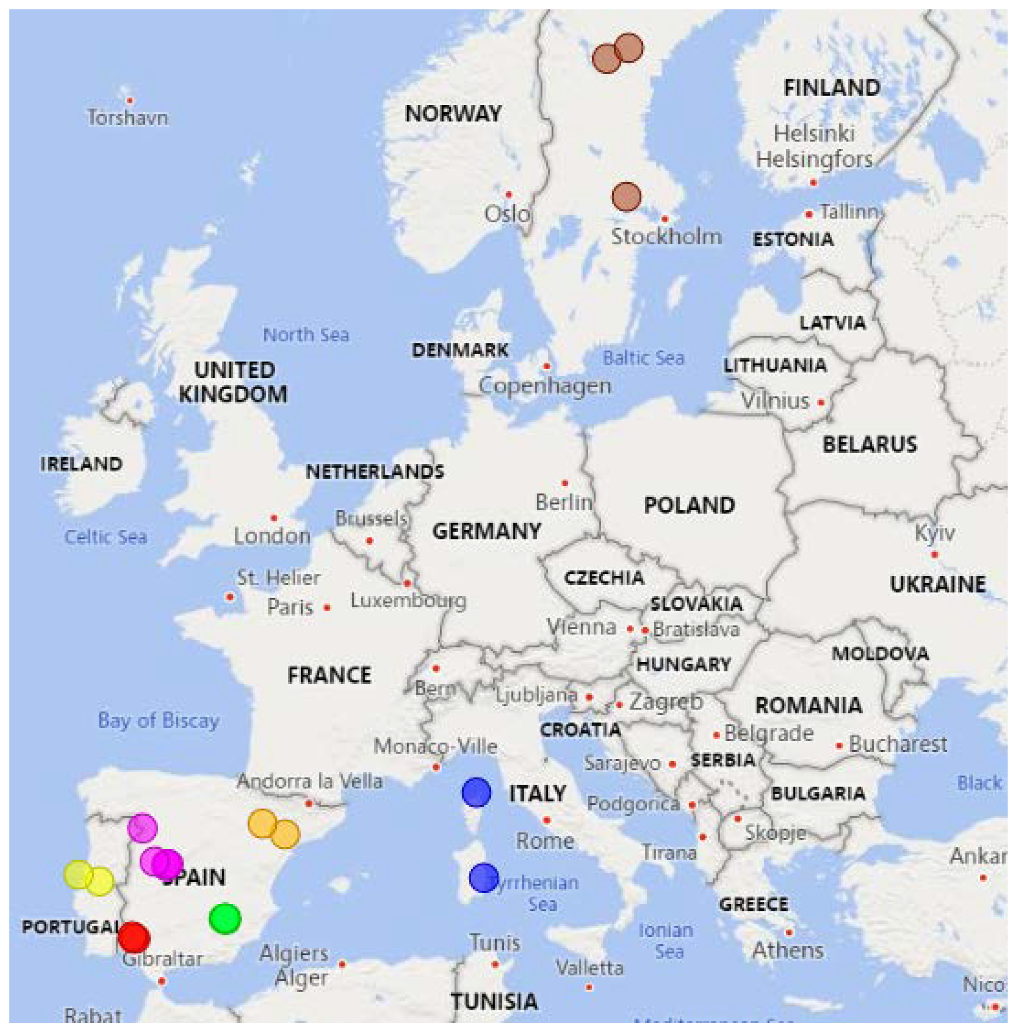
In this paper, 21 Copernicus EMS grading maps have been collected from 5 European regions: Portugal, Spain, France, Italy, and Sweden. The Sentinel-2 data have been downloaded at the highest resolution. Then, the AoIs were split into 7 folds, according to two different constraints: (i) a fold must include at least two AoIs, and (ii) areas of interest must be geographically close. A representation of the geographical distribution of the wildfire-affected regions and their categorization in folds is shown in Figure 1.
Once downloaded, satellite acquisitions are images of dimensions . W and H are the acquisition Width and Height, respectively, and are up to pixels. D, the Depth, is the number of spectral bands, which is 12 for Sentinel-2 L2A imagery. Copernicus EMS grading maps are images of size , having the same dimensions of the satellite acquisitions. Each pixel of the Copernicus annotation determines the damage severity level of the corresponding pixel—at the same row and column—of the Sentinel-2 acquisition. Details about the collection, especially the Copernicus EMS annotations, the dates in which Sentinel-2 data were acquired, and the fold they were assigned to are reported in Appendix A. Moreover, in order to allow the proposed method to generalize among different kinds of vegetation, another aspect considered in the dataset is the heterogeneity of land use, which includes inland areas with dense vegetation (i.e., red fold), areas characterized by cropland and small or sparse trees (i.e., fucsia fold), coastal areas (i.e., blue fold) and rural areas with little or no vegetation (i.e., yellow fold). A detail of the land use distribution for every AoI included in the dataset is reported in the Appendix B.
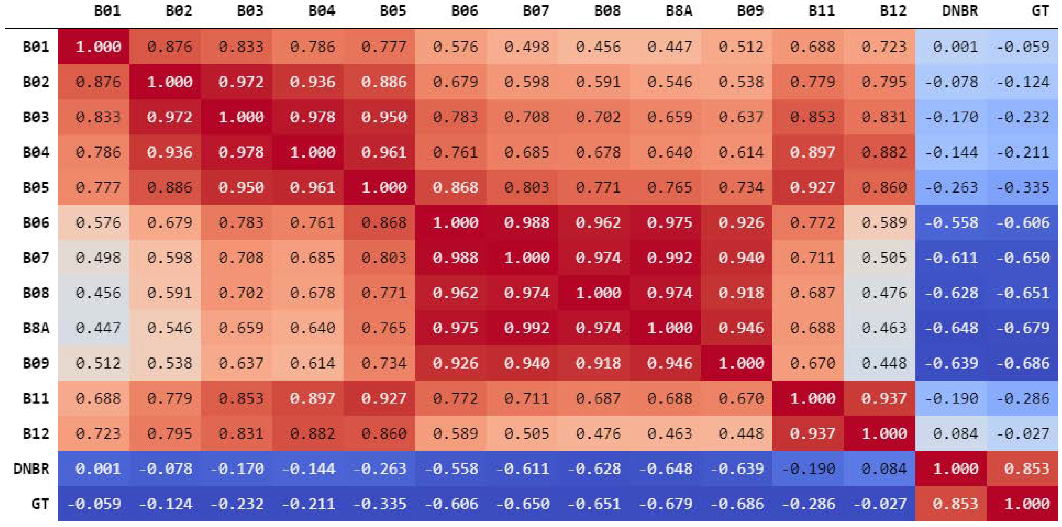
In order to assess the spectral bands that can provide useful information for the detection of the damage severity, the Pearson’s correlation between the bands of the collected AoIs, the dNBR, and the ground truth EMS damage level have been investigated. We considered also the dNBR index because it is widely used in previous papers and we want to understand if that index, based on pre- and post-imagery, is more correlated to the target variable than the Sentinel-2 bands. The Pearson’s correlation is a measure computed between two variables and it ranges between −1 and 1. High correlation is determined at the extremes of its domain: a highly positive or a highly negative value means the two variables are directly or indirectly related, respectively. More in detail, no correlation is expressed by 0, it is low for values between −0.35 and 0.35, and medium to strong for the remaining values [37]. In order to compute the correlation coefficient, a transformation was applied to each image and annotation. Each spectral band, the dNBR, and the EMS severity grading maps (ground truth, GT), all having dimensions , have been flattened into a vector of length , in order to resemble statistical variables. In the following, we use GT (Ground Truth) to refer to the target variable of this analysis, i.e., the damage severity level. As shown in Figure 2, the spectral bands presenting noticeable correlations (medium or high) with both the dNBR index and the target variable GT (i.e., the damage severity level) are B06, B07, B08, B8A, and B09. Except for B09, the other bands are known in the literature for the computation of the most used indexes for fire detection, such as the Burned Area Index (BAI) [17], the Burned Area Index for Sentinel2 (BAIS2) [38], the Normalized Burn Ratio (NBR) [39], the Normalized Burn Ratio 2 (NBR2) [16], and the Mid-Infrared Burned Index (MIRBI) [40]. Moreover, B07 and B08 are used for the computation of (i) the vegetation index, Normalized Difference Vegetation Index (NDVI) [41], and (ii) the water index, Normalized Difference Water Index (NDWI) [42], respectively. Moreover, it is worth considering the high correlation between dNBR and GT, which is coherent with the literature and confirms the dNBR to be a good estimator of the GT. However, also the Sentinel-2 bands are characterized by high correlation values with respect to the target variable and they can be obtained by considering one single post-fire image, whereas two imagery (pre- and post-fire) are needed to compute the dNBR index.
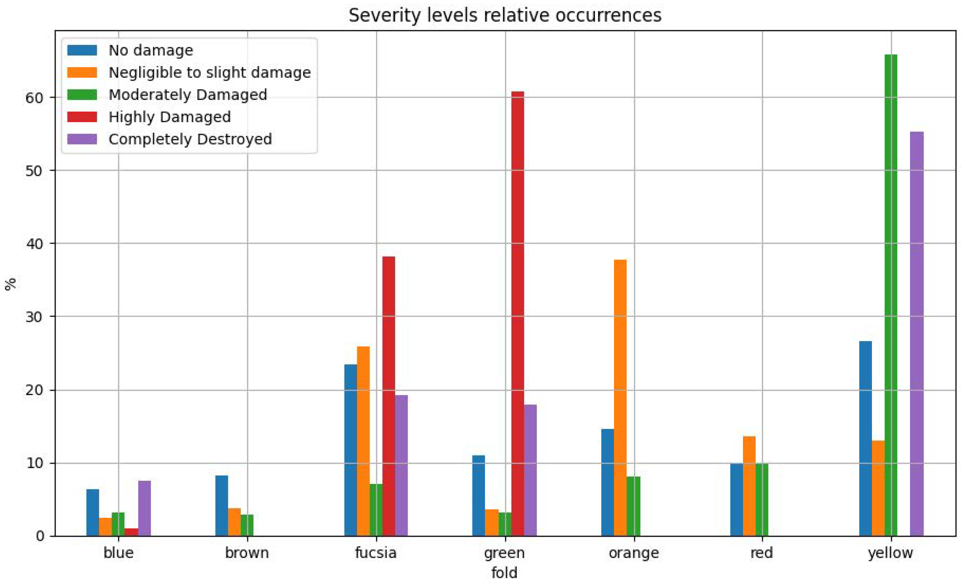
In Section 2.4, the new proposed approach, which leverages on Convolutional Neural Networks (CNNs), will be introduced. Given the huge interest from the scientific community in such algorithms, a common practice is to use consolidated approaches by adapting the general methodology to the investigated domain. As most CNNs, the input size is reduced due to computational performances and hardware limitations during the training phase. The high-resolution images retrieved from Sentinel-Hub (and consequently, the grading maps) have dimensions up to 5000 × 5000 pixels, but the image size is too big to be processed by a CNN in one shot (due to GPU memory limitations), therefore it needs to be re-adapted. In this paper, we opted for preserving all the provided information by tiling the original acquisitions in smaller crops of size 480 × 480 pixels, maintaining the spectral information as provided by Sentinel-Hub. Moreover, only the crops containing at least one pixel classified as burned (a damage severity level between 1 and 4) have been included in the dataset. In the end, the dataset contains a total of 135 crops, distributed in folds as follows; blue fold: 8, brown fold: 9, fucsia fold: 30, green fold: 16, orange fold: 18, red fold: 12, yellow fold: 42. As easily predictable, the dataset’s folds present unbalanced EMS damage severity levels, as shown in Figure 3.
2.3. Problem Statement
This work focuses on the estimation of the EMS damage severity levels for the sub-areas of an area hit by a new wildfire. More formally, given a post-fire Sentinel-2 L2A satellite acquisition (an image of 12 spectral bands) of an area that has been hit by a new wildfire the goal is to predict a continuous value in the range for each pixel of the input post-fire image, in order to approximate the Copernicus EMS damage severity grading map values, whose severity levels are natural numbers within the same range. The problem is configured as a regression task because the target variable is a numerical feature, which is used to represent ordered severity values. A set of training post-wildfire imagery related to past wildfires, for which the value of the target variable is known, is used to train a predictive model that is then applied to perform the prediction for the pixels of the new post-wildfire imagery.
2.4. Methodology
As briefly introduced in Section 2.2, one of the most recent and promising approaches developed in the computer vision field is U-Net [43]. The model, inspired from a Convolutional Neural Network presented to the Computer Vision for Pattern Recognition conference [44], was originally employed in the medical field for the segmentation of biological cells and for the analysis of MRI scans for the detection of a number of pathologies [45,46,47].
The network concatenates two branches: a contracting path and an expansive path, giving it the u-shaped architecture. The contracting path is a classical convolutional network, consisting of repeated application of convolutions, each followed by a rectified linear unit (ReLU) and a max-pooling operation. During the contraction, the spatial information is reduced while feature information is increased. The expansive path combines both the features and the spatial information through a sequence of up-convolutions and concatenations with high-resolution features from the contracting path. The original version takes as input one grayscale image of dimension 572 × 572 pixels and it outputs a binary mask of 388 × 388 pixels. The input is oversized compared to the output: that choice was made to give some extra context to include information of the biological cells outside exceeding the border of the considered tile. In the context of this paper, the dimension of a burned area is not predictable, therefore the authors opted for setting the network’s width and height input and output dimensions to 480 × 480 pixels for each of the 12 spectral bands. In the end, the U-Net’s input dimension is set to 480 × 480 × 12 pixels.
One of the main contributions of this study is the modification of the original U-Net, empowering its ability to distinguish between ordered classes, as in the case of damage severity. The classical U-Net was proposed for solving a segmentation task, being able to identify a specified entity in an image. Therefore, it is able to recognize relations and features (i.e., borders and gradients) among the pixel values belonging to the searched entity. Conversely, in the context of this work, the goal appears to be more complex and it can be split into two sub-tasks: (i) to identify areas affected by fire, and (ii) to determine damage severity in the burned areas. In the first sub-task, the goal is to distinguish burned areas from unburned regions, like in a classical segmentation task (classification task). The second sub-task takes into account the areas affected by the fire and discriminates between four consequent levels the severity of the damage (regression task). The two sub-tasks are solved with two different building blocks: the “Binary Classification U-Net” and the “Regression U-Net”. In both the building blocks, the output map is a matrix of dimensions 480 × 480, where each element refers to the pixel at the same position of the input tile. In the proposed solution, the two building blocks are combined together to outperform the prediction quality of the approach based only on the Regression U-Net block.
First, the Binary Classification U-Net is trained for segmentation purposes: given a satellite image of 12 channels and a resolution of 480 × 480, the network assigns to each pixel the probability of belonging to a burned area thanks to the application of the softmax activation function. Thus, the generated output is a binary segmentation map of size 480 × 480 with values {0, 1} (i.e., unburned or burned), where each pixel is assigned to the class with the highest probability. Second, the Regression U-Net is used to provide the severity level estimation. Given the input satellite image, the model generates as output a map of the same size as the input with values in range [0, 4]. Both architectures are based on the U-Net model, with the only difference on the softmax activation function [48] at the output layer of the Binary Classification U-Net, which is absent in the Regression U-Net, and the loss functions used during the training process, as described in Section 2.6.
By combining the two mentioned building blocks differently, we have considered three different approaches:
- A regression-only approach, in which only the Regression U-Net is used.
- A parallel approach, namely, Parallel U-Net, in which the two building blocks are used separately in parallel. The final output is obtained by the mathematical multiplication of the two outputs as shown in Figure 4.
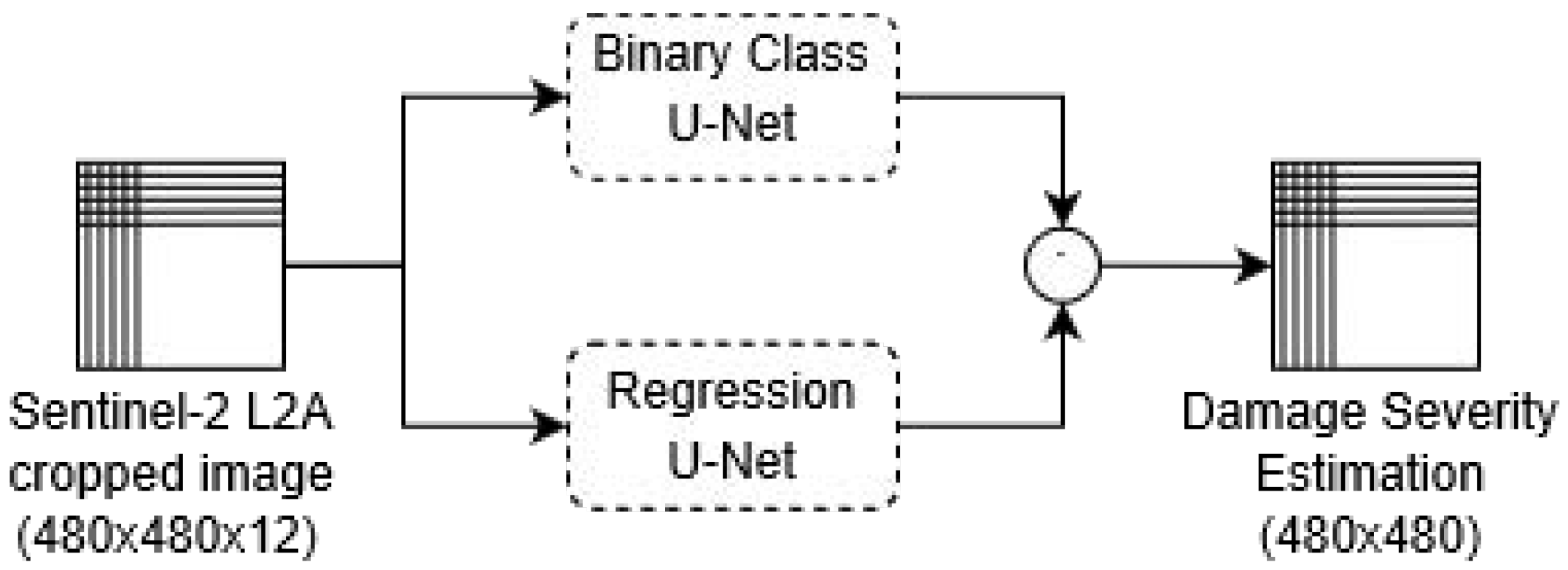
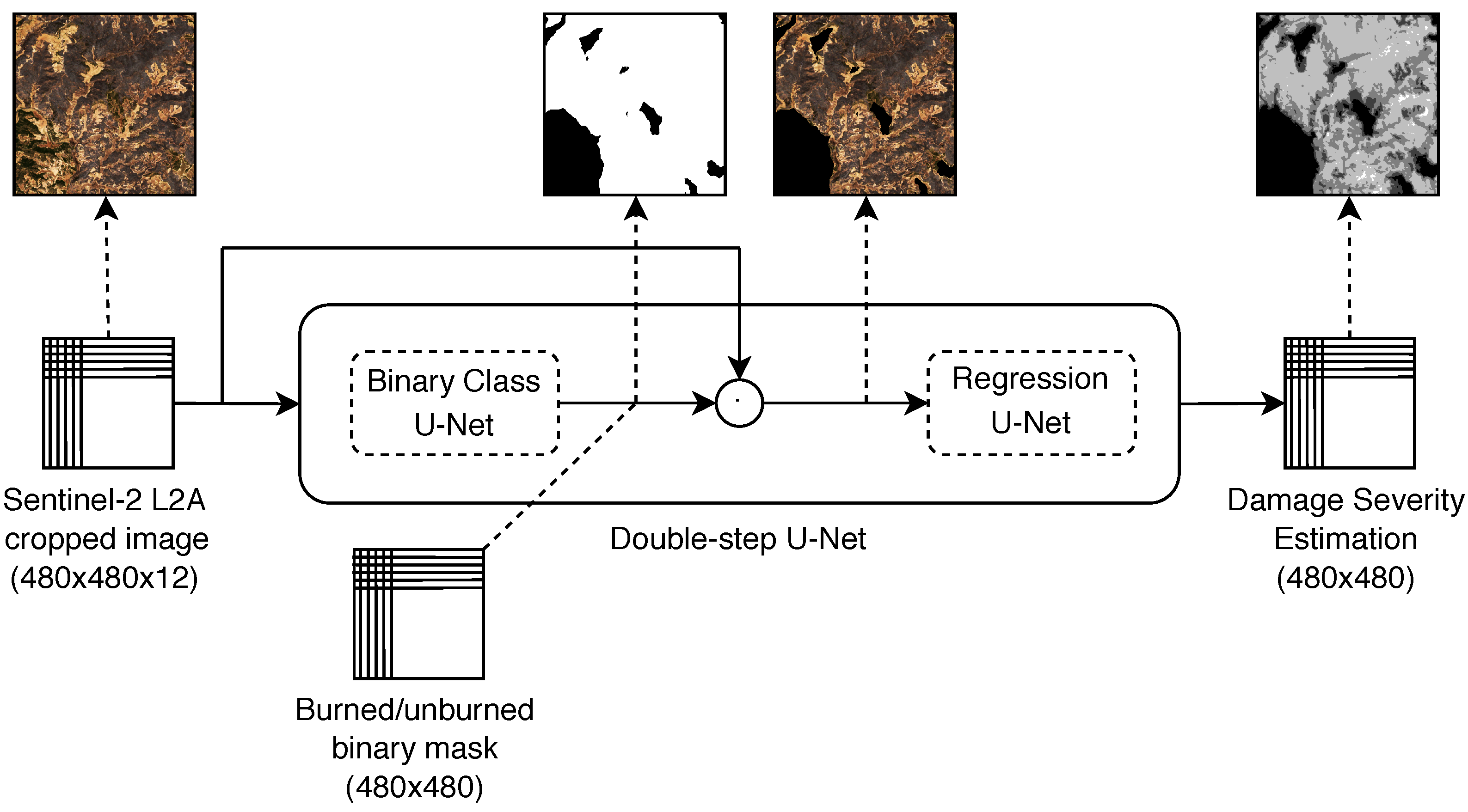
- A two-step approach, namely, Double-step U-Net, in which the building blocks are concatenated. First, the binary segmentation model is used to predict the burned area regions in the input tile. The binary prediction is used to filter the input and isolate the burned regions, thus generating the input tile for the Regression U-Net, which provides the damage severity estimation. Figure 5 shows the simplified architecture of the proposed solution with sample images, where for satellite imagery only the RGB channels are shown for simplicity.
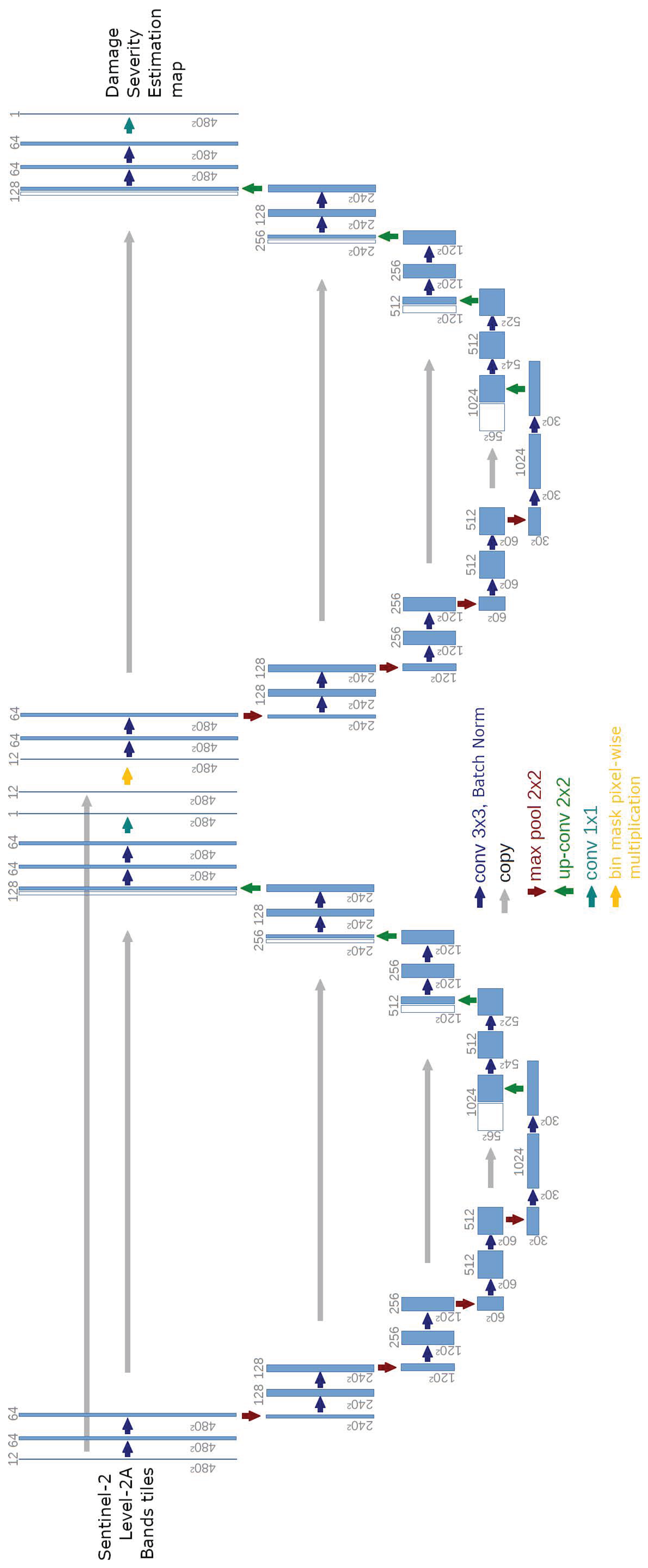
A detailed version of the Double-step U-Net architecture is shown in Appendix C.
2.5. Frameworks and Tools
In this section, the hardware components of the workstation used to run the experiments are introduced, as well as a detail of the software packages used to develop this work.
Geospatial data from Copernicus EMS was processed using the GDAL software library [49] to determine AoIs’ coordinates and to identify the precise regions affected by forest wildfires and the corresponding severity levels. Sentinel-Hub services were used to collect Sentinel-2 data.
Satellite imagery was processed through Python with OpenCV and scikit-image [50] libraries. Data analysis was performed through scikit-learn [51], whereas neural network models were developed and trained using PyTorch framework [52]. All the software packages and versions are specified in Table 2.
The experiments were run on a workstation with an Intel Core i9-7940X @ 3.10GHz with 128GB of RAM and 4x GTX 1080Ti.
2.6. Experiments
Training neural networks is a complex and computationally intensive task, which requires proper data preparation steps and hyperparameters selection. This section presents the experiments performed, detailing the training and the evaluation procedures adopted.
As introduced in Section 2.2, the satellite acquisitions were divided into seven folds. The grouping criteria was chosen by considering geographical distance among the position of the acquisitions, in order to include in the same fold geographically close regions that could share similar morphology and land cover aspects, such as vegetation types, infrastructures, and agricultural areas. The models’ performances were evaluated through a cross-validation approach, using the Root Mean Squared Error as the evaluation metric. At each iteration, five folds are used as the training set, one as the validation set, and the remaining fold as the test set. The validation set is used to assess the model’s performance for the early stopping regularization criteria, discussed later in this section. A common prerequisite in supervised learning algorithms is that the training, validation and test data arise from the same distribution and are independent and identically distributed [53]. Therefore, in order to work properly, a validation set should resemble the data distribution of the test set. However, as shown in Figure 1, each fold presents a unique distribution of severity levels. In a real situation, there is no chance to know the distribution of severity levels a priori. Therefore, the choice fell on a fold which contains all severity levels and which could generalise the most, presenting a distribution of severity levels which tends mostly to a uniform distribution. Considering all those aspects, we chose the “fucsia” fold as the validation set for each test set, except for itself: in that case, we chose the “green” fold.
To improve models generalization, data augmentation was applied on the training set of each fold. During the training process, synthetic data was generated at each epoch from the 480 × 480 tiles by randomly applying four transformations in sequence to each image: random rotation, random horizontal flip, random vertical flip, and random shear. Each transformation has a specific probability to be applied. Rotation and shear effects were performed with randomly generated angles within specific ranges, differently for each image in each epoch. For reproducibility purposes, random generation operations were performed using the same seed in each training.
The transformations and their respective parameters are shown in Table 3.
All the training phases were performed using Adam optimizer with a learning rate of , 50 epochs and a batch size of 8. Two different models were considered in this study:
- the single U-Net: it is trained for the regression task. The Mean Squared Error (MSE) was used as a loss function. This model will be referred to as the baseline;
- the Double-Step U-Net: it is trained in two steps: First, only the Binary Classification U-Net is trained with Dice loss function [54], keeping the weights of the regression model frozen. Second, the Regression U-Net was trained with Mean Squared Error (MSE) loss function. In this second step, the weights of the binary classification model are frozen.
To validate the approach, an ablation study will be presented. First, the performance obtained by the Binary U-Net on each fold will be reported. Then, the choice to link the two networks consecutively will be justified comparing Double-Step U-Net with the simplified Parallel U-Net model.
During the training process, three techniques for regularization were adopted: early stopping, dropout, and batch normalization. Early stopping was implemented to avoid overfitting and to stop the training process in case no further improvements were seen in the validation loss. A patience of 5 epochs was used with minimum improvements of on the validation loss. At the end of each training process, the model’s best weights determined by the early stopping mechanism were restored. Dropout layers were enabled during the training process before each transposed convolution with a probability of 25%. Moreover, after each convolutional layer, batch normalization was performed. Moreover, to guarantee the reproducibility of the tests, in each training of the cross-validation process the networks were initialized with the same weights generated from the same seed number, using a normal distribution and the Glorot initialization [55]. The two subtasks introduced in Section 2 are evaluated as follows.
- The binary classification between burned and unburned areas is evaluated with Precision, Recall, and F1-Score metrics [56]. Precision considers the purity of the predictions: among the pixels predicted as belonging to a certain class, e.g., belonging to a burned region, it indicates the percentage of matches with the GT. Recall verifies the ability of the estimator to recognize all the pixels belonging to a certain class, specified in the GT. Therefore, given the whole set of pixels belonging to a certain class (referring to the GT), the recall is the percentage of correctly predicted pixels among the whole set. The F1-Score is the harmonic mean between Precision and Recall. It is as a measure of accuracy with the property to consider the class imbalance.
- The estimation of damage severity, concerning the distinction between 5 severity levels, is evaluated with Root Mean Squared Error (RMSE) metric. Given the ordinal relationship between damage severity levels, the RMSE gives a measure of distance between the prediction and the ground truth.
3. Results
This section shows and comments on the results of the experiments described in Section 2.6. First, U-Net’s ability to distinguish between burned and unburned areas will be assessed. Then, the performance achieved to predict the damage severity level by the Double-Step U-Net, the Parallel U-Net and the Simple U-Net will be compared. Furthermore, their scores will be compared with the performance obtained by the dNBR-based solution, the reliable estimator largely adopted in the literature. Finally, the approaches will be discussed analyzing their average prediction error for each severity level.
In the binary classification task, the Binary U-Net achieved good performances, as shown in Table 4. According to the F1-Score, the approach was on the average able to classify correctly burned and unburned pixels (sub-areas) for the wildfires in every fold, except for the brown one, which contains data acquired from Sweden. In detail, in that fold, the Binary U-Net showed high Recall, but poor Precision: this means that the network overestimated the burned areas, predicting many false positives. The choice to use the same fold (fucsia, containing data acquired in Spain) as the validation set, helped us to understand the limits of applicability of the approach for data acquired far from the test set. Therefore, training and test areas with strong differences, in terms of geology or land cover aspects, can prevent the neural network from working properly in the binary classification task. However, this limitation is mitigated in the regression problem, discussed below in this section.
A detailed performance report for the Single U-Net, the Parallel U-Net, and the Double-Step U-Net in every fold for the estimation of damage severity task is shown Table 5. As mentioned in Section 2.4, the three approaches use solely post-fire satellite acquisition for making their predictions. The table presents the RMSE evaluated on every fold, for every severity level, reported as an ordinal number for the sake of space. Severity levels are mapped as follows; 0 stands for No damage, 1 stands for Negligible to slight damage, 2 stands for Moderately Damaged, 3 stands for Highly damaged, and 4 stands for Completely destroyed. In a first analysis, we do not consider the dNBR column, but we focus only on the three networks performances. The best score for each row, considering only the U-Net-based approaches, is marked with the star symbol (☆). Compared to the Single U-Net, the approaches in which the outputs of the Binary U-Net and Regression U-Net are combined showed better overall performances. The Double-Step U-Net is the most accurate in the discrimination between severity levels (1 to 4), achieving best results in 5 folds out of 7 (blue, fucsia, green, orange, and yellow). The only exception is for the brown fold because the Regression U-Net is strongly dependent on the Binary U-Net’s performance. However, the RMSE values of the brown fold for the Double-Step U-Net result to be comparable to the RMSE values of other folds (i.e., orange and yellow), and they are better than the ones of the consolidated approach based on dNBR. Therefore, Double-Step U-Net result to be also robust for regions presenting strong differences from the ones that are used to train the model.
Considering the dNBR in the evaluation, the best performances per row in Table 5 are marked with the dagger symbol (). In order to compare the dNBR with the GT, its values were thresholded according to the default values [23]. In this case, best results vary from fold to fold, but generally, they are matched by U-Net based approaches. It must be considered that the dNBR is computed using both pre- and post-fire acquisitions, whereas U-Net’s approaches consider only post-fire acquisitions. In order to summarize the performance, the average RMSE value for each severity level is shown in Table 6. Compared to the Single U-Net, the Double-Step U-Net results to be a better approach, achieving the best RMSE on each severity level. Moreover, with reference to the dNBR, the Double-Step U-Net achieves comparable performance, with a noticeable improvement for the detection of the unburned area (severity 0), but using only half of the information. The reason behind the success of Double-Step U-Net is hidden in the problem split. First, the neurons of the Binary U-Net are employed to identify burned regions. Its prediction will mask the spectral values of unburned regions, leaving only the information related to burned areas to the Regression U-Net. Therefore, the latter network will employ its neurons in finding differences between correlated values (severity levels 1 to 4).
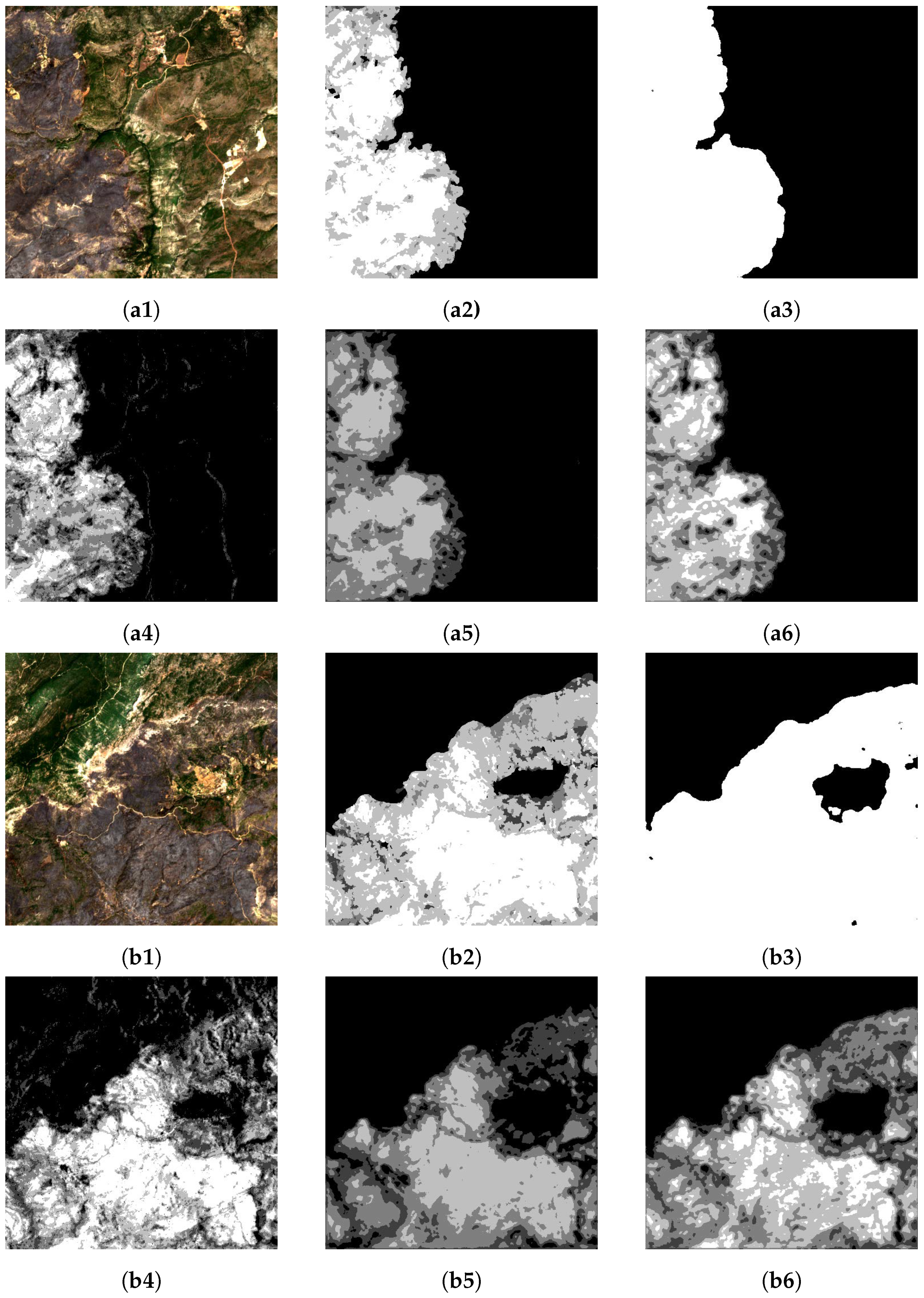
It is worth mentioning that the masking operation performed by the Binary U-Net prediction introduces a new and uncommon value in the spectral information fed as input to the Regression U-Net: the 0 value. Areas identified as unburned will be “cancelled” by replacing their original value with 0, that is not present in nature. Therefore, a bad classification from the Binary U-Net can lead the Regression U-Net to make more mistakes because it will consider 0-valued-regions as unburned and every other unburned region not detected by the Binary U-Net will be considered as burned. In Figure 6, a comparison between predictions of dNBR, Single U-Net, and Double-Step U-Net is shown in two areas of the green fold. At a first glance, delineating the wildfire contours just looking at the RGB acquisition (pictures a1 and b1) seems feasible, but assigning different severity levels appears to be more challenging. In both the acquisitions, the Binary U-Net predictions resulted to be highly accurate (pictures a3 and b3), compared to the Copernicus EMS annotation (GT, pictures a2 and b2). The dNBR (pictures a4 and b4) show a good match with the GT, except for some noise in the vast unburned regions. The Single U-Net (pictures a5 and b5) correctly identifies the burned region and the contours of different burned areas, but it tends to underestimate the severity. In the end, the Double-Step U-Net (pictures a6 and b6) improves the prediction of the Single U-Net, resulting to be more similar to the GT. The time required by the Double-Step U-Net to perform the damage severity evaluation using one NVIDIA GTX 1080 Ti on an input tile of size 100 km × 100 km is, considering the highest spatial resolution available (reported in Table 1), 28 s on average. The time required to predict the severity level estimation by the proposed deep learning model for an image of 480 × 480 resolution with 12 spectral bands is inferior to 1 s.
4. Conclusions
This work introduces the application of a convolutional neural network, namely, U-Net for the estimation of the damage severity of regions affected by wildfires from satellite imagery. Compared to the literature, which commonly uses pre-fire and post-fire satellite acquisitions, this approach only makes use of post-fire data. Moreover, our approach results to be location-independent for the assessed European regions, and possibly for all the areas presenting common land-use as the AoIs presented in this work), being able to process geographically distributed satellite imagery. Furthermore, a modified version of U-Net named Double-Step U-Net, is created and introduced to improve the performance of the standard method. The approaches have been validated across five European regions, within 21 manually annotated wildfire events. As a result, Double-Step U-Net outperformed U-Net and achieved comparable performance to the thresholded dNBR, which is computed using both pre- and post-wildfire satellite acquisitions.
Future works will assess the contribution of other information, like Synthetic-aperture radar (SAR) data provided by Sentinel-1 data, or the Digital Elevation Maps (DEM) to improve the performances of Double-Step U-Net for distinguishing between wildfire severity levels. Moreover, the approach can be adapted and evolved to analyse the daily wildfire expansion, in order to provide a risk map for the potential areas that could be affected in the near future. Therefore, areas more likely to be affected by severe damage can be identified earlier, in order to let decision-makers to conduct better disaster response management and to limit overall damages.
Author Contributions
Conceptualization, A.F. and L.C.; methodology, A.F. and L.C.; software, L.C. and A.F.; validation, A.F., L.C. and P.G.; formal analysis, A.F., L.C., and P.G.; investigation, A.F. and L.C.; resources, A.F. and L.C.; data curation, L.C. and A.F.; writing–original draft preparation, A.F., L.C. and P.G.; writing–review and editing, P.G.; visualization, A.F. and L.C.; supervision, P.G.; funding acquisition, A.F. and P.G. All authors have read and agreed to the published version of the manuscript.
Funding
This research was partially funded by the European Commission through the SHELTER project, grant agreement n.821282. The APC was funded by Politecnico di Torino.
Acknowledgments
Data used in this work is provided by the European Space Agency (ESA). The authors thank Grega Milcinski (Sentinel-Hub) and Raffaele Rigoli (ESA) for their prompt support.
Conflicts of Interest
The authors declare no conflicts of interest.
Appendix A
Dataset—Legend:
- ISO stands for ISO-3166 Country Code (https://www.iso.org/obp/ui/#search&3166);
- EMSR stands for Copernicus Emergency Management Service (EMS) - Rapid Mapping (R) Activation Code (https://emergency.copernicus.eu/mapping);
- BB_TL_LON and BB_TL_LAT is the couple of coordinates (LONgitude, LATitude) of the Bounding Box (BB) for the Top Left (TL) corner;
- BB_BR_LON and BB_BR_LAT is the couple of coordinates (LONgitude, LATitude) of the Bounding Box (BB) for the Bottom Right (BR) corner;
- PRE Date and POST Date stand for Pre Fire acquisition Date, and Post fire acquisition Date, respectively. They specify the date in which the Sentinel-2 satellite registered information related to the specified bounding box, which is compliant with the constraints of availability and cloud coverage specified in Section 2.2.
- FOLD indicates in which fold the product belongs to, according to the colors represented in Figure 1.

Table A1.
Areas of Interest (AoIs) considered in this work. Each AoI reports information about the Country (ISO code), the grading map identifier for Copernicus EMS (EMSR), the coordinates of the AoI’s top-left and bottom-right corners, the Pre-fire (PRE Date) and Post-fire (POST Date) Sentinel-2 acquisition dates, and the related fold.
| ISO | EMSR | BB_TL_LON | BB_TL_LAT | BB_BR_LON | BB_BR_LAT | PRE Date | POST Date | FOLD |
|---|---|---|---|---|---|---|---|---|
| FR | 221_01 | 9.300647504 | 42.886608180 | 9.505183140 | 42.763508590 | 06-07-2017 | 15-08-2017 | blue |
| IT | 371_01 | 9.644467300 | 39.921109700 | 9.687531600 | 39.856982400 | 18-07-2018 | 18-07-2019 | |
| SE | 290_03 | 16.260418860 | 59.853342900 | 16.321359390 | 59.828218650 | 20-05-2018 | 09-06-2018 | brown |
| 298_02 | 16.361547000 | 63.140440500 | 16.447381400 | 63.099673880 | 26-06-2018 | 24-07-2018 | ||
| 298_06 | 15.357103890 | 62.915099290 | 15.574015210 | 62.833943810 | 27-06-2018 | 24-07-2018 | ||
| ES | 248_01 | −6.196452795 | 41.659029510 | −6.009019170 | 41.544015950 | 14-07-2017 | 08-08-2017 | fucsia |
| 248_03 | −5.635075322 | 40.498431780 | −5.506317882 | 40.418039390 | 02-04-2017 | 04-09-2017 | ||
| 248_04 | −5.095913397 | 40.401377180 | −5.017491612 | 40.352353570 | 01-07-2017 | 20-08-2017 | ||
| 248_05 | −4.999988815 | 40.416147790 | −4.903491087 | 40.355830440 | 15-08-2017 | 04-09-2017 | ||
| 368_01 | −5.078459714 | 40.337887420 | −4.823074137 | 40.208122740 | 18-05-2018 | 01-07-2019 | ||
| ES | 216_01 | −2.372395304 | 38.474711270 | −2.314204884 | 38.425632380 | 28-06-2017 | 04-08-2017 | green |
| 216_02 | −2.314223218 | 38.474528270 | −2.256145364 | 38.425540850 | 03-07-2017 | 04-08-2017 | ||
| 216_04 | −2.314236645 | 38.425632380 | −2.256299384 | 38.376741980 | 03-07-2017 | 04-08-2017 | ||
| 216_05 | −2.430549330 | 38.455364920 | −2.372358909 | 38.406286030 | 03-07-2017 | 04-08-2017 | ||
| ES | 365_01 | 0.412424949 | 41.454152670 | 0.770854806 | 41.165836340 | 31-05-2019 | 30-06-2019 | orange |
| 373_01 | −0.630882068 | 41.824559980 | −0.508149384 | 41.754863330 | 18-07-2018 | 25-07-2019 | ||
| ES | 302_01 | −6.673627731 | 37.809332970 | −6.460693904 | 37.671156100 | 16-07-2018 | 05-08-2018 | red |
| 302_06 | −6.603647894 | 37.733337620 | −6.530111345 | 37.685598470 | 16-07-2018 | 05-08-2018 | ||
| 302_07 | −6.530284692 | 37.733470790 | −6.456643427 | 37.685736730 | 16-07-2018 | 05-08-2018 | ||
| PT | 250_01 | −9.163435178 | 40.036735710 | −8.705635612 | 39.636755460 | 27-09-2017 | 17-10-2017 | yellow |
| 372_04 | −8.192177749 | 39.796433080 | −7.948217694 | 39.609595860 | 13-08-2018 | 24-07-2019 |
Appendix B
Dataset Land use—Legend: Land use details for the areas of interest considered in the dataset Table A2 and Table A3. They are specified in the grading maps cartouche, using the hectare (ha) as unit of measurement. The land use types are specified as follows (Land use types used in this work refer to the official Copernicus EMS notation, available at https://emergency.copernicus.eu/mapping/ems/domains):
- Residential/Industrial: urban areas involving residential or industrial buildings;
- Arable land: also specified as cropland, non-irrigated arable land areas, permanently irrigated land, and rice fields;
- Grassland: natural grassland;
- Forests: broad-leaved forest, coniferous forest, mixed forest;
- Heterogeneous agricultural areas: annual crops associated with permanent crops, complex cultivation, land principally occupied by agriculture, agro-forestry areas;
- Open spaces with little or no vegetation: beaches, dunes, sand plains, bare rock, sparsely vegetated areas, and glaciers;
- Pastures: ground covered with grass or herbage, used or suitable for the grazing of livestock;
- Permanent Crops: vineyards, fruit trees and berry plantations, olive groves;
- Shrub and/or herbaceous vegetation association: natural grassland, moors, and heathland, Sclerophyllous vegetation, transitional woodland shrub;
- Inland wetlands: inland marshes, peatbogs;
- Woodland shrub: transitional woodland shrub.
For sake of space the table is split in two parts: the first reports land use attributes from “Arable land” to “Open spaces with little or no vegetation”, the other from “Pastures” to “Woodland”.
Table A2.
Land use details for the AoIs considered in this work. For the sake of space, this table is partial, and continues in Table A3. It reports, in hectares: Residential/Industrial areas, Arable lands, Grasslands, Forests, Heterogeneous agricultural areas, and Open spaces with little or no vegetation. For each land use type, the areas affected by fire are reported (Burned).
| EMSR | Res. / Ind. (ha) | Arable Land (ha) | Grassland (ha) | Forests (ha) | Het. agric. (ha) | Open sp. (ha) | ||||||
|---|---|---|---|---|---|---|---|---|---|---|---|---|
| Burnt | AoI | Burnt | AoI | Burnt | AoI | Burnt | AoI | Burnt | AoI | Burnt | AoI | |
| 221_01 | n.d. | n.d. | n.d. | n.d. | n.d. | n.d. | n.d. | n.d. | n.d. | n.d. | n.d. | n.d. |
| 371_01 | 3.5 | 29 | 123.3 | 646.8 | 36.5 | 98.9 | 503.8 | |||||
| 290_03 | 115.6 | 17.8 | 570.3 | 86.7 | ||||||||
| 298_02 | 262.2 | 197.4 | 1062.7 | 56.4 | ||||||||
| 298_06 | 350.5 | 7661 | ||||||||||
| 248_01 | 112.1 | 1048.1 | 7562.7 | 84.1 | 1404.8 | |||||||
| 248_03 | 286.2 | 2617.4 | 247.8 | 2589.8 | ||||||||
| 248_04 | 85.2 | 573 | 36.4 | 488 | ||||||||
| 248_05 | 58.8 | 247.6 | 1330.4 | 5.6 | 186.4 | |||||||
| 368_01 | 12.1 | 32.2 | 58.2 | 8279.2 | 10.8 | 1233.3 | 1010.8 | |||||
| 216_01 | 43 | 185 | 169.7 | 244.3 | 46.5 | 103.7 | ||||||
| 216_02 | 37 | 265.6 | ||||||||||
| 216_04 | 466 | 646.5 | 185.3 | |||||||||
| 216_05 | 57 | 3.3 | 129.4 | 26.2 | 1872.3 | |||||||
| 365_01 | 365.1 | 1323.3 | 1538 | 12,281.3 | 2287 | 35,995.5 | ||||||
| 373_01 | 208.3 | 2899.4 | 173 | 1702.9 | 122.6 | 810 | ||||||
| 302_01 | 761 | 630.2 | 708 | 7653.5 | 24.7 | 3148.8 | ||||||
| 302_06 | 24 | 4650 | 29.3 | 377.8 | 744.7 | 27.2 | ||||||
| 302_07 | 3 | 54 | 54.9 | 1597.5 | 50.3 | |||||||
| 250_01 | 120.7 | 1129.3 | 7677 | 50.8 | 2472.8 | 636.2 | 2356.4 | |||||
| 372_04 | n.d. | n.d. | n.d. | n.d. | n.d. | n.d. | n.d. | n.d. | n.d. | n.d. | n.d. | n.d. |
Table A3.
Land use details for the AoIs considered in this work. For the sake of space, this table is partial, and continues from Table A2. It reports, in hectares: Pastures areas, Permanent crop lands, Shrubs or herbaceous vegetation areas, Inland wetlands areas, and Woodlands. For each land use type, the areas affected by fire are reported (Burned).
| EMSR | Pastures (ha) | Perm. Crops (ha) | Shrubs / herb. (ha) | In. Wetlands (ha) | Woodland (ha) | |||||
|---|---|---|---|---|---|---|---|---|---|---|
| Burnt | AoI | Burnt | AoI | Burnt | AoI | Burnt | AoI | Burnt | AoI | |
| 221_01 | n.d. | n.d. | n.d. | n.d. | n.d. | n.d. | n.d. | n.d. | n.d. | n.d. |
| 371_01 | 25 | 267.9 | 381.8 | 936.3 | ||||||
| 290_03 | 13.9 | 18.3 | 120.1 | 14 | ||||||
| 298_02 | 7.9 | 112 | ||||||||
| 298_06 | 52.2 | 1626.2 | ||||||||
| 248_01 | 1642.4 | 8521.42 | 56.1 | 1989.9 | ||||||
| 248_03 | 674.7 | 2980.1 | 836 | 1565.6 | ||||||
| 248_04 | 437.4 | 2353.5 | 47.3 | 220.6 | ||||||
| 248_05 | 588.9 | 1513 | 166.7 | 2457.5 | ||||||
| 368_01 | 1708.6 | 2896.1 | 1471.3 | 15,130.6 | ||||||
| 216_01 | 796.1 | 924 | 860.9 | 1482.4 | ||||||
| 216_02 | 658.2 | 1834.5 | 172.8 | 643 | ||||||
| 216_04 | 99.7 | 821.6 | 980.1 | |||||||
| 216_05 | 236.1 | 148.8 | 483.82 | |||||||
| 365_01 | 316.8 | 6695.8 | 880.2 | 8877.5 | 38.3 | |||||
| 373_01 | 366.3 | 918.3 | ||||||||
| 302_01 | 199.4 | 499.8 | 958 | 13,469.9 | ||||||
| 302_06 | 391.9 | 960.4 | ||||||||
| 302_07 | 83.6 | 2578.9 | ||||||||
| 250_01 | 300 | 642 | 1172.2 | 6596.2 | ||||||
| 372_04 | n.d. | n.d. | n.d. | n.d. | n.d. | n.d. | n.d. | n.d. | n.d. | n.d. |
Appendix C
Figure A1.
Double-Step U-Net architecture.

References
- European Commission. More Countries Than Ever Hit by Forest Fires in 2018. October 2019. Available online: https://ec.europa.eu/jrc/en/news/more-countries-ever-hit-forest-fires-2018 (accessed on 22 February 2020).
- European Union. Copernicus Sentinel-2 Mission. 2020. Available online: https://emergency.copernicus.eu/ (accessed on 20 February 2020).
- Ban, Y.; Zhang, P.; Nascetti, A.; Bevington, A.R.; Wulder, M.A. Near Real-Time Wildfire Progression Monitoring with Sentinel-1 SAR Time Series and Deep Learning. Sci. Rep. 2020, 10, 1–15. [Google Scholar] [CrossRef] [PubMed] [Green Version]
- Pinto, M.M.; Libonati, R.; Trigo, R.M.; Trigo, I.F.; DaCamara, C.C. A deep learning approach for mapping and dating burned areas using temporal sequences of satellite images. ISPRS J. Photogramm. Remote Sens. 2020, 160, 260–274. [Google Scholar] [CrossRef]
- Giglio, L.; Boschetti, L.; Roy, D.P.; Humber, M.L.; Justice, C.O. The Collection 6 MODIS burned area mapping algorithm and product. Remote Sens. Environ. 2018, 217, 72–85. [Google Scholar] [CrossRef]
- Hardtke, L.A.; Blanco, P.D.; del Valle, H.F.; Metternicht, G.I.; Sione, W.F. Semi-automated mapping of burned areas in semi-arid ecosystems using MODIS time-series imagery. Int. J. Appl. Earth Obs. Geoinf. 2015, 38, 25–35. [Google Scholar] [CrossRef]
- De Araujo, F.M.; Ferreira, L.G. Satellite-based automated burned area detection: A performance assessment of the MODIS MCD45A1 in the Brazilian savanna. Int. J. Appl. Earth Obs. Geoinf. 2015, 36, 94–102. [Google Scholar] [CrossRef]
- Hughes, M.; Kaylor, S.; Hayes, D. Patch-based forest change detection from Landsat time series. Forests 2017, 8, 166. [Google Scholar] [CrossRef]
- Boschetti, L.; Roy, D.P.; Justice, C.O.; Humber, M.L. MODIS–Landsat fusion for large area 30 m burned area mapping. Remote Sens. Environ. 2015, 161, 27–42. [Google Scholar] [CrossRef]
- Ramo, R.; Chuvieco, E. Developing a random forest algorithm for MODIS global burned area classification. Remote Sens. 2017, 9, 1193. [Google Scholar] [CrossRef] [Green Version]
- Ramo, R.; Garcia, M.; Rodriguez, D.; Chuvieco, E. A data mining approach for global burned area mapping. Int. J. Appl. Earth Obs. Geoinf. 2018, 73, 39–51. [Google Scholar] [CrossRef]
- Shan, T.; Wang, C.; Chen, F.; Wu, Q.; Li, B.; Yu, B.; Shirazi, Z.; Lin, Z.; Wu, W. A Burned Area Mapping Algorithm for Chinese FengYun-3 MERSI Satellite Data. Remote Sens. 2017, 9, 736. [Google Scholar] [CrossRef] [Green Version]
- Bin, W.; Ming, L.; Dan, J.; Suju, L.; Qiang, C.; Chao, W.; Yang, Z.; Huan, Y.; Jun, Z. A Method of Automatically Extracting Forest Fire Burned Areas Using Gf-1 Remote Sensing Images. In Proceedings of the IGARSS 2019-2019 IEEE International Geoscience and Remote Sensing Symposium, Yokohama, Japan, 28 July–2 August 2019; pp. 9953–9955. [Google Scholar]
- Verhegghen, A.; Eva, H.; Ceccherini, G.; Achard, F.; Gond, V.; Gourlet-Fleury, S.; Cerutti, P. The potential of Sentinel satellites for burnt area mapping and monitoring in the Congo Basin forests. Remote Sens. 2016, 8, 986. [Google Scholar] [CrossRef] [Green Version]
- Roy, D.P.; Huang, H.; Boschetti, L.; Giglio, L.; Yan, L.; Zhang, H.H.; Li, Z. Landsat-8 and Sentinel-2 burned area mapping-A combined sensor multi-temporal change detection approach. Remote Sens. Environ. 2019, 231, 111254. [Google Scholar] [CrossRef]
- Roteta, E.; Bastarrika, A.; Padilla, M.; Storm, T.; Chuvieco, E. Development of a Sentinel-2 burned area algorithm: Generation of a small fire database for sub-Saharan Africa. Remote Sens. Environ. 2019, 222, 1–17. [Google Scholar] [CrossRef]
- Stavrakoudis, D.; Katagis, T.; Minakou, C.; Gitas, I.Z. Towards a fully automatic processing chain for operationally mapping burned areas countrywide exploiting Sentinel-2 imagery. In Proceedings of the Seventh International Conference on Remote Sensing and Geoinformation of the Environment (RSCy2019). International Society for Optics and Photonics, Paphos, Cyprus, 18–21 March 2019; Volume 11174, p. 1117405. [Google Scholar]
- Filipponi, F. Exploitation of Sentinel-2 Time Series to Map Burned Areas at the National Level: A Case Study on the 2017 Italy Wildfires. Remote Sens. 2019, 11, 622. [Google Scholar] [CrossRef] [Green Version]
- Farasin, A.; Nini, G.; Garza, P.; Rossi, C. Unsupervised Burned Area Estimation through Satellite Tiles: A Multimodal Approach by Means of Image Segmentation Over Remote Sensing Imagery. CEUR-WS. 2019. Available online: http://ceur-ws.org/Vol-2466/paper7.pdf (accessed on 23 June 2020).
- Farasin, A.; Colomba, L.; Palomba, G.; Nini, G.; Rossi, C. Supervised Burned Areas delineation by means of Sentinel-2 imagery and Convolutional Neural Networks. In Proceedings of the 17th International Conference on Information Systems for Crisis Response and Management (ISCRAM 2020), Virginia Tech, Blacksburg, VA, USA, 24–27 May 2020. [Google Scholar]
- European Union. Copernicus EMS, Service Overview. 2020. Available online: https://emergency.copernicus.eu/mapping/ems/service-overview (accessed on 18 January 2020).
- Miller, J.D.; Thode, A.E. Quantifying burn severity in a heterogeneous landscape with a relative version of the delta Normalized Burn Ratio (dNBR). Remote Sens. Environ. 2007, 109, 66–80. [Google Scholar] [CrossRef]
- Key, C.H.; Benson, N.C. Landscape assessment (LA). In FIREMON: Fire Effects Monitoring and Inventory System; Lutes, D.C., Keane, R.E., Caratti, J.F., Key, C.H., Benson, N.C., Steve, S., Gangi, L.J., Eds.; Gen. Tech. Rep. RMRS-GTR-164-CD; Department of Agriculture, Forest Service, Rocky Mountain Research Station: Fort Collins, CO, USA, 2006; Volume 164. [Google Scholar]
- Navarro, G.; Caballero, I.; Silva, G.; Parra, P.C.; Vázquez, Á.; Caldeira, R. Evaluation of forest fire on Madeira Island using Sentinel-2A MSI imagery. Int. J. Appl. Earth Obs. Geoinf. 2017, 58, 97–106. [Google Scholar] [CrossRef] [Green Version]
- Saulino, L.; Rita, A.; Migliozzi, A.; Maffei, C.; Allevato, E.; Garonna, A.P.; Saracino, A. Detecting Burn Severity across Mediterranean Forest Types by Coupling Medium-Spatial Resolution Satellite Imagery and Field Data. Remote Sens. 2020, 12, 741. [Google Scholar] [CrossRef] [Green Version]
- Franco, M.G.; Mundo, I.A.; Veblen, T.T. Field-Validated Burn-Severity Mapping in North Patagonian Forests. Remote Sens. 2020, 12, 214. [Google Scholar] [CrossRef] [Green Version]
- Xu, W.; He, H.S.; Hawbaker, T.J.; Zhu, Z.; Henne, P.D. Estimating burn severity and carbon emissions from a historic megafire in boreal forests of China. Sci. Total Environ. 2020, 716, 136534. [Google Scholar] [CrossRef]
- Zheng, Z.; Wang, J.; Shan, B.; He, Y.; Liao, C.; Gao, Y.; Yang, S. A New Model for Transfer Learning-Based Mapping of Burn Severity. Remote Sens. 2020, 12, 708. [Google Scholar] [CrossRef] [Green Version]
- Gibson, R.; Danaher, T.; Hehir, W.; Collins, L. A remote sensing approach to mapping fire severity in south-eastern Australia using sentinel 2 and random forest. Remote Sens. Environ. 2020, 240, 111702. [Google Scholar] [CrossRef]
- Copernicus, European Space Agency (ESA). Copernicus Sentinel-2 Mission. 2020. Available online: https://sentinel.esa.int/web/sentinel/missions/sentinel-2 (accessed on 13 April 2020).
- Copernicus, European Space Agency (ESA). Sentinel-2 Level-1C Products. 2020. Available online: https://earth.esa.int/web/sentinel/user-guides/sentinel-2-msi/product-types/level-1c (accessed on 12 April 2020).
- Copernicus, European Space Agency (ESA). Sentinel-2 Level-1C Processing. 2020. Available online: https://earth.esa.int/web/sentinel/technical-guides/sentinel-2-msi/level-1c-processing (accessed on 13 April 2020).
- Copernicus, European Space Agency (ESA). Sentinel-2 Level-2A Products. 2020. Available online: https://sentinel.esa.int/web/sentinel/user-guides/sentinel-2-msi/processing-levels/level-2 (accessed on 13 April 2020).
- Copernicus, European Space Agency (ESA). Sentinel-2 Level-2A Processing. 2020. Available online: https://earth.esa.int/web/sentinel/technical-guides/sentinel-2-msi/level-2a/algorithm (accessed on 11 April 2020).
- Sinergise. Sentinel-Hub platform. 2020. Available online: https://www.sentinel-hub.com/ (accessed on 23 January 2020).
- Braaten, J.D.; Cohen, W.B.; Yang, Z. Automated cloud and cloud shadow identification in Landsat MSS imagery for temperate ecosystems. Remote Sens. Environ. 2015, 169, 128–138. [Google Scholar] [CrossRef] [Green Version]
- Linty, N.; Farasin, A.; Favenza, A.; Dovis, F. Detection of GNSS ionospheric scintillations based on machine learning decision tree. IEEE Trans. Aerosp. Electron. Syst. 2018, 55, 303–317. [Google Scholar] [CrossRef]
- Filipponi, F. BAIS2: Burned Area Index for Sentinel-2. Multidiscip. Digit. Publ. Inst. Proc. 2018, 2, 364. [Google Scholar] [CrossRef] [Green Version]
- Roy, D.P.; Boschetti, L.; Trigg, S.N. Remote sensing of fire severity: Assessing the performance of the normalized burn ratio. IEEE Geosci. Remote Sens. Lett. 2006, 3, 112–116. [Google Scholar] [CrossRef] [Green Version]
- Zanetti, M.; Marinelli, D.; Bertoluzza, M.; Saha, S.; Bovolo, F.; Bruzzone, L.; Magliozzi, M.L.; Zavagli, M.; Costantini, M. A high resolution burned area detector for Sentinel-2 and Landsat-8. In Proceedings of the 2019 10th International Workshop on the Analysis of Multitemporal Remote Sensing Images (MultiTemp), Shanghai, China, 5–7 August 2019; pp. 1–4. [Google Scholar]
- Frampton, W.J.; Dash, J.; Watmough, G.; Milton, E.J. Evaluating the capabilities of Sentinel-2 for quantitative estimation of biophysical variables in vegetation. ISPRS J. Photogramm. Remote Sens. 2013, 82, 83–92. [Google Scholar] [CrossRef] [Green Version]
- Yang, X.; Zhao, S.; Qin, X.; Zhao, N.; Liang, L. Mapping of urban surface water bodies from Sentinel-2 MSI imagery at 10 m resolution via NDWI-based image sharpening. Remote Sens. 2017, 9, 596. [Google Scholar] [CrossRef] [Green Version]
- Ronneberger, O.; Fischer, P.; Brox, T. U-net: Convolutional networks for biomedical image segmentation. In International Conference on Medical Image Computing And Computer-Assisted Intervention; Springer: Cham, Switzerland, 2015; pp. 234–241. [Google Scholar]
- Long, J.; Shelhamer, E.; Darrell, T. Fully convolutional networks for semantic segmentation. In Proceedings of the IEEE Conference on Computer Vision and Pattern Recognition, Boston, MA, USA, 7–12 June 2015; pp. 3431–3440. [Google Scholar]
- Zhang, L.; Mohamed, A.A.; Chai, R.; Guo, Y.; Zheng, B.; Wu, S. Automated deep learning method for whole-breast segmentation in diffusion-weighted breast MRI. J. Magn. Reson. Imaging 2020, 51, 635–643. [Google Scholar] [CrossRef]
- Sriram, S.A.; Paul, A.; Zhu, Y.; Sandfort, V.; Pickhardt, P.J.; Summers, R.M. Multilevel UNet for pancreas segmentation from non-contrast CT scans through domain adaptation. In Medical Imaging 2020: Computer-Aided Diagnosis; International Society for Optics and Photonics: Houston, TX, USA, 2020; Volume 11314, p. 113140K. [Google Scholar]
- Dutta, J.; Chakraborty, D.; Mondal, D. Multimodal Segmentation of Brain Tumours in Volumetric MRI Scans of the Brain Using Time-Distributed U-Net. In Computational Intelligence in Pattern Recognition; Springer: Singapore, 2020; pp. 715–725. [Google Scholar]
- Goodfellow, I.; Bengio, Y.; Courville, A. Deep Learning; MIT Press: Cambridge, MA, USA, 2016. [Google Scholar]
- GDAL/OGR CContributors. GDAL/OGR Geospatial Data Abstraction Software Library; Open Source Geospatial Foundation: Chicago, IL, USA, 2020. [Google Scholar]
- Van der Walt, S.; Schönberger, J.L.; Nunez-Iglesias, J.; Boulogne, F.; Warner, J.D.; Yager, N.; Gouillart, E.; Yu, T. Scikit-image: Image processing in Python. PeerJ 2014, 2, e453. [Google Scholar] [CrossRef]
- Buitinck, L.; Louppe, G.; Blondel, M.; Pedregosa, F.; Mueller, A.; Grisel, O.; Niculae, V.; Prettenhofer, P.; Gramfort, A.; Grobler, J.; et al. API design for machine learning software: Experiences from the scikit-learn project. In Proceedings of the ECML PKDD Workshop: Languages for Data Mining and Machine Learning, Prague, Czech Republic, 23–27 September 2013; pp. 108–122. [Google Scholar]
- Paszke, A.; Gross, S.; Massa, F.; Lerer, A.; Bradbury, J.; Chanan, G.; Killeen, T.; Lin, Z.; Gimelshein, N.; Antiga, L.; et al. PyTorch: An Imperative Style, High-Performance Deep Learning Library. In Advances in Neural Information Processing Systems 32; Curran Associates, Inc.: Vancouver, BC, Canada, 2019; pp. 8024–8035. [Google Scholar]
- Ng, A. Proceedings of the Twenty-First International Conference on Machine Learning; Association for Computing Machinery: New York, NY, USA, 2004. [Google Scholar]
- Soomro, T.A.; Hellwich, O.; Afifi, A.J.; Paul, M.; Gao, J.; Zheng, L. Strided U-Net model: Retinal vessels segmentation using dice loss. In Proceedings of the 2018 IEEE Digital Image Computing: Techniques and Applications (DICTA), Canberra, Australia, 10–13 December 2018; pp. 1–8. [Google Scholar]
- Glorot, X.; Bengio, Y. Understanding the difficulty of training deep feedforward neural networks. In Proceedings of the Thirteenth International Conference on Artificial Intelligence and Statistics, Sardinia, Italy, 13–15 May 2010; pp. 249–256. [Google Scholar]
- Flach, P. Machine Learning: The Art and Science of Algorithms That Make Sense of Data; Cambridge University Press: Cambridge, UK, 2012. [Google Scholar]
Figure 1.
Map of the areas hit by wildfires considered in this study, split by fold. Circles determine the position of the considered wildfires, while each circle colour identifies a specific fold: circles of the same color identify areas of interest attributed to the same fold.
Figure 1.
Map of the areas hit by wildfires considered in this study, split by fold. Circles determine the position of the considered wildfires, while each circle colour identifies a specific fold: circles of the same color identify areas of interest attributed to the same fold.

Figure 2.
Correlation Matrix computed on burned areas. Spectral Bands B01–B12 refer to the post-fire Sentinel-2 acquisition, dNBR is the Delta Normalized Burn Ratio, and GT is the severity level target variable (i.e., the Copernicus EMS grading map Ground Truth).
Figure 2.
Correlation Matrix computed on burned areas. Spectral Bands B01–B12 refer to the post-fire Sentinel-2 acquisition, dNBR is the Delta Normalized Burn Ratio, and GT is the severity level target variable (i.e., the Copernicus EMS grading map Ground Truth).

Figure 3.
Severity level distribution among each fold. For each severity level, the percentage of pixels with the considered level is computed within each fold.
Figure 3.
Severity level distribution among each fold. For each severity level, the percentage of pixels with the considered level is computed within each fold.

Figure 4.
Parallel U-Net simplified architecture. The damage severity estimation is computed by filtering the Regression U-Net output with the burned/unburned binary mask.
Figure 4.
Parallel U-Net simplified architecture. The damage severity estimation is computed by filtering the Regression U-Net output with the burned/unburned binary mask.

Figure 5.
Double-Step U-Net simplified architecture. The damage severity estimation is computed in two steps: burned area identification through the Binary Class U-Net and damage severity estimation by means of Regression U-Net. The Regression U-Net receives as input the Sentinel-2 L2A image filtered with the binary segmentation mask.

Figure 6.
Wildfire severity level predictions. The severity levels range from black (severity 0) to white (severity 4). (a1,b1) Sentinel L2A acquisition; (a2,b2) Copernicus EMS grading map (GT); (a3,b3) Binary mask generated by the Binary U-Net: black and white colors indicate unburned and burned regions, respectively; (a4,b4) Thresholded dNBR, obtained from pre and post-fire acquisitions; (a5,b5) Single U-Net prediction; (a6,b6) Double-Step U-Net prediction.

Table 1.
Sentinel-2 spectral bands description.
| Band | Description | Central Wavelength (m) | Spatial Resolution (m) |
|---|---|---|---|
| 1 | Coastal aerosol | 0.443 | 60 |
| 2 | Blue | 0.490 | 10 |
| 3 | Green | 0.560 | 10 |
| 4 | Red | 0.665 | 10 |
| 5 | Vegetation red edge | 0.705 | 20 |
| 6 | Vegetation red edge | 0.740 | 20 |
| 7 | Vegetation red edge | 0.783 | 20 |
| 8 | Near Infrared (NIR) | 0.842 | 10 |
| 8A | Narrow NIR | 0.865 | 20 |
| 9 | Water vapour | 0.940 | 60 |
| 10 | Short wavelength infrared (SWIR) | 1.375 | 60 |
| 11 | SWIR | 1.610 | 20 |
| 12 | SWIR | 2.190 | 20 |
Table 2.
Software packages and versions installed.
| Software/Library | Version |
|---|---|
| python | 3.6.9 |
| numpy | 1.18.2 |
| pandas | 1.0.3 |
| xlrd | 1.2.0 |
| matplotlib | 3.2.1 |
| scikit-learn | 0.22.2 |
| scikit-image | 0.16.2 |
| OpenCV | 4.2.0 |
| PyTorch | 1.4.0 |
| torchvision | 0.5.0 |
| CUDA | 10.1 |
Table 3.
Data augmentation parameters.
| Transformation | Probability | Parameters |
|---|---|---|
| Random rotation | 50% | Angle: [−50°, +50°] |
| Random horizontal flip | 50% | - |
| Random vertical flip | 50% | - |
| Random shear | 50% | Angle: [−20°, +20°] |
Table 4.
Binary U-Net cross-validation results for the binary classification subtask.
| Bin. U-Net | Fold | ||||||
|---|---|---|---|---|---|---|---|
| Blue | Brown | Fucsia | Green | Orange | Red | Yellow | |
| Precision | 0.91 | 0.45 | 0.93 | 0.99 | 0.71 | 0.84 | 0.78 |
| Recall | 0.95 | 0.98 | 0.98 | 0.91 | 0.99 | 0.99 | 0.99 |
| F-Score | 0.93 | 0.61 | 0.95 | 0.95 | 0.82 | 0.91 | 0.87 |
Table 5.
Cross-validation performance per fold. () indicates the best RMSE per severity category among the three U-Net versions. () indicates the best RMSE per severity category, dNBR included.
Table 5.
Cross-validation performance per fold. () indicates the best RMSE per severity category among the three U-Net versions. () indicates the best RMSE per severity category, dNBR included.
| Fold | Severity | Performance (RMSE) | |||
|---|---|---|---|---|---|
| dNBR | Single U-Net | Parallel U-Net | Double-Step U-Net | ||
| Blue | 0 | 0.78 | 1.06 | 0.27 | |
| 1 | 1.07 | 0.89 | 0.89 | ||
| 2 | 1.23 | 0.71 | 0.80 | ||
| 3 | 0.82 | 0.63 | 0.65 | ||
| 4 | 0.96 | 1.44 | |||
| Brown | 0 | 0.65 | 0.22 | 0.47 | |
| 1 | 0.97 | 0.94 | 0.94 | ||
| 2 | 1.01 | 0.86 | |||
| 3 | 0.70 | 0.39 | |||
| 4 | 1.28 | 1.49 | |||
| Fucsia | 0 | 0.82 | 0.39 | 0.24 | |
| 1 | 1.37 | 1.40 | 1.41 | ||
| 2 | 1.12 | 1.35 | 1.35 | ||
| 3 | 1.10 | 0.97 | 0.97 | ||
| 4 | 1.67 | 1.28 | 1.49 | ||
| Green | 0 | 0.20 | 0.28 | 0.18 | |
| 1 | 1.03 | 0.92 | |||
| 2 | 1.78 | 1.76 | |||
| 3 | 1.46 | 1.87 | 1.90 | ||
| 4 | 1.09 | 1.57 | 1.58 | ||
| Orange | 0 | 0.40 | 0.43 | ||
| 1 | 1.68 | 1.68 | |||
| 2 | 1.04 | 1.14 | 1.14 | ||
| 3 | - | - | - | - | |
| 4 | - | - | - | - | |
| Red | 0 | 0.20 | 0.21 | 0.33 | |
| 1 | 1.21 | ||||
| 2 | 0.80 | 0.97 | |||
| 3 | - | - | - | - | |
| 4 | 1.96 | 1.96 | |||
| Yellow | 0 | 1.31 | 0.37 | 0.54 | |
| 1 | 0.84 | 1.04 | |||
| 2 | 1.24 | 0.89 | 0.89 | ||
| 3 | - | - | - | - | |
| 4 | 1.70 | 1.71 | |||
Table 6.
Average performance for severity level. () indicates the best RMSE per severity category among the three U-Net versions. () indicates the best RMSE per severity category, dNBR included.
Table 6.
Average performance for severity level. () indicates the best RMSE per severity category among the three U-Net versions. () indicates the best RMSE per severity category, dNBR included.
| Severity | Overall Per-Class Performance (RMSE) | |||
|---|---|---|---|---|
| dNBR | Single U-Net | Parallel U-Net | Double-Step U-Net | |
| 0 | 0.62 | 0.42 | 0.35 | |
| 1 | 1.07 | 1.05 | ||
| 2 | 1.09 | 1.01 | 1.02 | |
| 3 | 1.02 | 0.95 | 0.97 | |
| 4 | 1.45 | 1.46 | ||
© 2020 by the authors. Licensee MDPI, Basel, Switzerland. This article is an open access article distributed under the terms and conditions of the Creative Commons Attribution (CC BY) license (http://creativecommons.org/licenses/by/4.0/).
Share and Cite
MDPI and ACS Style
Farasin, A.; Colomba, L.; Garza, P. Double-Step U-Net: A Deep Learning-Based Approach for the Estimation of Wildfire Damage Severity through Sentinel-2 Satellite Data. Appl. Sci. 2020, 10, 4332. https://doi.org/10.3390/app10124332
AMA Style
Farasin A, Colomba L, Garza P. Double-Step U-Net: A Deep Learning-Based Approach for the Estimation of Wildfire Damage Severity through Sentinel-2 Satellite Data. Applied Sciences. 2020; 10(12):4332. https://doi.org/10.3390/app10124332
Chicago/Turabian StyleFarasin, Alessandro, Luca Colomba, and Paolo Garza. 2020. "Double-Step U-Net: A Deep Learning-Based Approach for the Estimation of Wildfire Damage Severity through Sentinel-2 Satellite Data" Applied Sciences 10, no. 12: 4332. https://doi.org/10.3390/app10124332
Note that from the first issue of 2016, this journal uses article numbers instead of page numbers. See further details here.