Performance Modeling of Ultraviolet Atmospheric Scattering of Different Light Sources Based on Monte Carlo Method

Featured Application

UV laser non-line-of-sight communication and detection; Transmission of ultraviolet laser and LED in the atmosphere.

Abstract

Since the atmosphere has a strong scattering effect on ultraviolet light, the transmission of non-line-of-sight (NLOS) signals can be realized in the atmosphere. In previous articles, ultraviolet (UV) light atmospheric scattering has been characterized by many scattering models based on spot light sources with uniformly distributed light intensity. In order to explore the role of light sources in atmospheric transmission, this work proposed a UV light atmospheric transport model under different types of light source, including light-emitting diode (LED), laser, and ordinary light sources, based on the Monte Carlo point probability method. The simulation of the light source in the proposed model is a departure from the use of a light source with uniform intensity distribution in previous articles. The atmospheric transmission efficiency of different light sources was calculated and compared with the data of existing models. The simulation results showed that the type of light source can significantly change the shape of the received signal and the received energy density. The Monte Carlo (MC) point probability method dramatically reduced the calculation time and the number of photons. The transmission characteristics of different ultraviolet light sources in the atmosphere provide a theoretical foundation for the design of ultraviolet detection and near-ultraviolet signal communication in the future.

1. Introduction

Due to its strong scattering and absorption characteristics in the atmosphere and its low background noise, ultraviolet light has been widely used in short-range atmospheric non-line-of-sight optical communication [1,2,3], near-field wind-field detection [4], aircraft landing aid [5], atmospheric parameter measurement [6], and networking aspects [7] in recent years, in both to theoretical and experimental studies.

The atmosphere is mainly composed of air molecules and aerosols. There are two main types of ultraviolet light scattering that occur in the atmosphere: Mie scattering (aerosols) and Rayleigh scattering (molecules) [8]. UV light contains three spectral bands, UVA (320–400 nm), UVB (280–320 nm), and UVC (200–280 nm). Different UV spectral bands lead to different SSA (single scattering albedo) and AAOD (absorption optical depth) values [9]. These two parameters are the main items measured in many experimental contexts [10,11,12,13,14].

Studies on UV none-line-of- sight (NLOS) communication mainly deal with UV devices, channel models, physical layer issues, and networking [3,15]. All these areas, without exception, relate to the transmission of ultraviolet light in atmosphere, which is mainly characterized by the shape of the received signal and the received energy density. For UV light sources, mercury lamps and xenon flash lamps were used for communication in early experimental studies. UV LEDs and lasers have become a research hot-spot in recent experimental research. However, there is currently little theoretical research regarding the influence of the light source on the received signal in UV communication and detection.

By reviewing previous relevant studies, various research methods for UV atmospheric scattering channel modeling were identified. The ellipsoidal coordinate was used to solve the single-scattering issue in References [16,17]. Subsequently, the coplanar [18,19] and non-coplanar transmission models [20,21] were proposed. In addition, in reference [22,23], the characteristics of UV atmospheric scattering in turbulent have been comprehensively studied. The above-mentioned theoretical models all assume that the light source is a spot with uniform intensity distribution. In fact, the light intensities from different light sources change in a variety of ways with viewing angle. Therefore, we wanted to further explore the effect of the light source on the received signal. For experimental studies, an LED array was used as a light source in reference [24]. And the black background noise and path loss were measured through experiments on the test bench. The pulse-broadening effect in atmospheric transmission was experimentally characterized using a narrow-pulse ultraviolet laser in Reference [25]. UV LEDs and avalanche photodiodes were used, respectively, for NLOS UV communication in References [26,27]. It was shown in Reference [28] that a square matrix receiver was proposed to study the spatial diversity in a new way. These experiments applied empirical methods and the numerical simulation of light sources needs to be further explored. The Monte Carlo point probability method is an efficient and time-saving technique for this purpose.

In this article, in order to explore the influence of different light sources on the received signal, models of different light sources were first established by using the curves of the lights’ intensity distributions. In other words, the initial distributions of large numbers of photons were used to generate simulations for different light sources. The trajectories of large numbers of photons were then recorded by MC point probability method. By changing different geometric parameters, the received irradiance levels of different light sources were compared in single and multiple scattering. The coplanar and non-coplanar issues were also considered.

2. Monte Carlo Point Probability Model and the Modeling of Light Sources

Based on these studies, this paper explored the pulses acquired at the receiver under different initial photon distributions, both coplanar and non-coplanar. Simulations of different light sources (mainly including LEDs, collimated lasers, and expanded laser beams) were conducted. The effect of the pulse broadening and the received energy density were evaluated.

In the case of multiple scattering and single scattering, respectively, we simulated the atmospheric transmission of UV light based on different kinds of light source. By changing the light intensity distribution of the light source and the geometric features of the transceiver ($\alpha$, ${\theta }_T$, ${\theta }_R$, ${\varphi }_T$, ${\varphi }_R$), we found that the light energy density of different light sources affected the received signal under the single-scattering mode. Compared with long-distance light transmission, the received energy increased more significantly through multiple scattering in short-range light propagation. Under the same divergence angle, the more concentrated the light energy density is, the higher the received energy efficiency. However, this led to greater sensitivity of the received energy to changes of the off-axis angle.

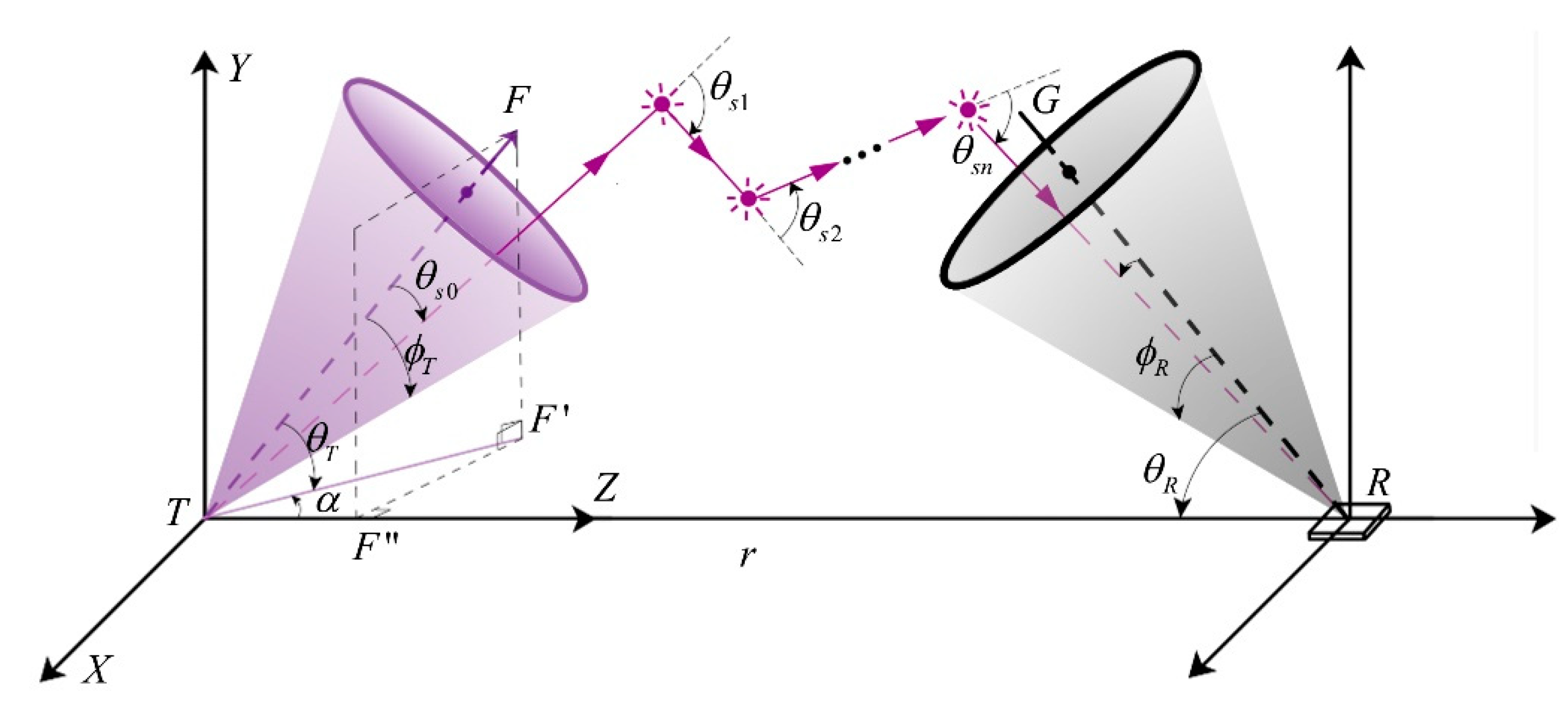
Figure 1 illustrates the process of ultraviolet light atmospheric transmission. T is the position of the emitting light source. A photon eventually reaches the receiver R (such as a photomultiplier tube, PMT) after it is scattered by aerosols and air molecules multiple times [29]. TF and RG indicate the central axes of the emergent light and the field of view (FOV), respectively. ${\varphi }_T$ and ${\varphi }_R$ are defined as the half-beam angle of the source and half-FOV angle, respectively. ${\theta }_T$ and ${\theta }_R$ represent the elevation angle of light source and receiver. ${\theta }_{sn}$ is the scattering angle after the nth scattering, and α refers to the off-axis angle. When $\alpha =0$, TF and RG are coplanar. ${\theta }_{s0}$ is the angle between the initial photon emission direction and TF. And r is the horizontal distance between T and R. TF’ is the projection of TF in the XTZ plane.

Because of the randomness of photons’ direction distribution and the limited receiving area of the detector, a large number of photons need to be traced for more accuracy. This greatly increases the running time of the program, as large numbers of photons are absorbed and have little contribution to the received signals. In the direct MC method, it is necessary to determine whether a photon reaches the detector at each scattering point, and calculate the weight of the photon after the last scattering. For the point probability method, we did not need to consider whether the scattered photons reached the detector; we just needed to calculate the point probability that the photon reached the detector at each scattering point [21].

The Monte Carlo point probability method simulates the propagation process of a large number of photons, and calculates the reception probability of the received photons. In this way, every scattering of each photon is valuable. Compared with the direct Monte Carlo method, it improves the photon utilization and reduces the program operation time, meaning that we can obtain the received light intensity as a function of time. The entire simulation process can be divided into three steps: the simulation of light, the propagation of the photons, and the reception of photons.

2.1. Photon Modeling of LED Light Sources

Part one: We first considered LEDs as the light source. We assumed that an LED is a Lambertian light source [30,31]. For the sake of simplicity, we assume it as a point light source. Lambertian light sources exist widely in nature, such as the sun, snow, etc. The beam divergence angle $2{\varphi }_T$ of the LED is generally 120°, which leads its luminous intensity to be very weak. However, it can be 60°, 34°, 30°, or even 12° when lens modules are installed. As a Lambertian light source, the irradiance of an LED light source can be expressed by Equation (1).

$$I\left(\theta \right)=I_0{\cos }^m\theta$$

(1)

where $I_0$ describes the intensity of light on the luminous axis of the LED light source and $\theta$ is the off-axis angle. m is the Lambertian emissivity, and it is defined by Equation (2).

$$m=-\ln \left(2\right)/\ln \left(\cos \left({\varphi }_T\right)\right)$$

(2)

Generally, in industrial contexts, ${\varphi }_T$ refers to the off-axis angle where the light intensity is equal to 0.5$I_0$. As shown in Figure 2, the light intensity of LEDs was more densely distributed in the paraxial region and we assumed that it had the same distribution of light intensity at different azimuths.

For the Monte Carlo simulation, we introduced the random number ${\xi }_{\theta }$, which satisfies uniform distribution on the interval [0,1], to simulate the initial emission state of a large number of photons. It can be obtained by the following expression.

$$H\left({\theta }_{\xi }\right)=\left({\displaystyle {\int }_0^{{\theta }_{\xi }}\frac{I\left(\theta \right)}{I_0}}\mathrm{d}\theta \right)/\left({\displaystyle {\int }_0^{\frac{\pi }{2}}\frac{I\left(\theta \right)}{I_0}}\mathrm{d}\theta \right)={\xi }_{\theta }$$

(3)

where ${\theta }_{\xi }$ is the off-axis angle uniquely determined by ${\xi }_{\theta }$. Since the left side of the equation is a hyper-geometric function, we cannot get the analytical solution of ${\theta }_{\xi }$. However, numerical solutions can be obtained by using spline interpolation method. We can obtain a series of numerical values $\left\{H\left({\theta }_1\right),H\left({\theta }_2\right),\dots ,H\left({\theta }_n\right)\right\}$ by taking equally spaced samples in $\left[0,\pi /2\right]$ and the spline interpolation expression $H\left({\theta }_{\xi }\right)$ can be obtained using the interp1 function in Matlab2014a.

2.2. Photon Modeling of Gaussian Laser Beam

Next, we considered the situation of a laser beam. The distribution of the intensity of a laser beam with its angle can be considered a Gaussian distribution [32,33]. In order to facilitate subsequent comparison with the classic communication model [28], we regarded the light source as a point light source. The brightness of the light source was uniform at all azimuth angles and the light intensity followed a normal distribution with the off-axis angle ${\xi }_{\mathsf{\Theta }}$, and ${\xi }_{\mathsf{\Theta }}~N\left(0,\sigma \right)$.

According to the 3σ-principle in the probability distribution, the probability that ${\xi }_{\mathsf{\Theta }}>3\sigma$ can be considered a small probability event. Let 3σ equal 1. We know that when $X~N\left(\mu ,{\sigma }^2\right)$, the probability density function (PDF) of X can be written as in Equation (4).

$$f\left(x,\mu ,\sigma \right)=\frac{1}{\sigma \sqrt{2\pi }}{e}^{-\frac{{\left(x-\mu \right)}^2}{2{\sigma }^2}}.$$

(4)

Furthermore, when $a$ and $b$ are real numbers,

$$aX+b~N\left(a\mu +b,{\left(a\sigma \right)}^2\right)$$

(5)

Therefore, if $Y~N\left(0,1\right)$, we have $X=Y/3~N\left(0,{\left(1/3\right)}^2\right)$. Remove the case where X = Y/3 is less than 0. The off-axis angle of the initial launch of each photon can be obtained from Equation (6).

$$\cos \left({\theta }_{{\xi }_{\mathsf{\Theta }}}\right)=1-{\xi }_{\mathsf{\Theta }}\left(1-\cos {\varphi }_T\right).$$

(6)

In conclusion, Figure 3 shows the relationship between the light intensity of different sources (with different ${\varphi }_T$) and the off-axis angle $\theta$.

2.3. Monte Carlo Point Probability Method

For the simulation of photon atmospheric transport, we used the Rayleigh phase function (Equation (5)) and generalized Henyey–Greenstein function (Equation (6)) to model the scattering caused by air molecules and aerosols, respectively, according to References [34,35].

$$P^{mie}\left(\mu \right)=\frac{1-g^2}{4\pi }\left[\frac{1}{{\left(1+g^2-2g\mu \right)}^{1.5}}+f\frac{3{\mu }^2-1}{2{\left(1+g^2\right)}^{1.5}}\right],$$

(7)

$$P^{ray}\left(\mu \right)=\frac{3\left[1+3\gamma +\left(1-\gamma \right){\mu }^2\right]}{16\pi \left(1+2\gamma \right)},$$

(8)

where $\mu =\cos {\theta }_s$, $\gamma =0.17$, $g=0.72$, and $f=0.5$. The total scattering phase function can be written as a weighted sum of the Rayleigh scattering (Equation (8)) and the Mie scattering phase function (Equation (7)).

$$P\left(\mu \right)=\frac{k_{sr}}{k_s}{p}^{ray}\left(\mu \right)+\frac{k_{sm}}{k_s}{p}^{mie}\left(\mu \right),$$

(9)

where $k_{sr}$ and $k_{sm}$ are the Rayleigh and Mie scattering coefficients, respectively. The total scattering coefficient $k_s=k_{sr}+k_{sm}$. As for the ultraviolet light at wavelength 266 nm, $k_{sm}=0.25{\mathrm{km}}^{-1}$, $k_{sr}=0.24{\mathrm{km}}^{-1}$ and the absorption coefficient can be set as $k_a=0.74{\mathrm{km}}^{-1}$ [36].

The algorithm of the MC point probability method includes four steps: photon emission, propagation, scattering, and detection.

Step 1. Emissions: For the scattering, the propagation direction vectors at the nth scattering position can be expressed as $\left(s_{xn},s_{yn},s_{zn}\right)$, and the acceptance probability is $P_{reci}$. The acquisition probability of all photons is assumed to be 1 at the beginning. Factors such as atmospheric absorption and the limit of the receiver’s FOV (field of view) can both make it much less than 1. The photon is initially emitted from point T and the coordinate is $\mathrm{T}\left(x_0,y_0,z_0\right)$. The direction cosines of a photon can be described by two angles ${\theta }_{\mathrm{si}}$ and ${\varphi }_{\mathrm{si}}$ in a 3D Cartesian coordinate system. The initial direction cosines can be derived by ${\theta }_{s0}$ and ${\varphi }_{s0}$.

Step 2. Propagation: The transmission distance of a photon needs to be determined during the simulation. According to Bill Lambert’s Law [27], the random propagation distance of photons between each scattering point can be set as

$$d=-\frac{\ln {\xi }_d}{k_e},$$

(10)

where ${\xi }_d$ is a random number that satisfies uniform distribution in the interval [0,1]. Thus, the coordinates of the nth scattering point can be obtained using (Equation (11)).

$$\{\begin{array}{c}{x}_n=x_0+{\displaystyle \sum _{i=0}^{n-1}{s}_{xi}{d}_i}\\ y_n=y_0+{\displaystyle \sum _{i=0}^{n-1}{s}_{yi}{d}_i}\\ z_n=z_0+{\displaystyle \sum _{i=0}^{n-1}{s}_{zi}{d}_i}\end{array},$$

(11)

Step 3. Scattering: According to Reference [37], the direction cosines $\left(s_{x,i+1},s_{y,i+1},s_{z,\mathrm{i}+1}\right)$ at the $i$th scattering point after scattering can be derived by $\left(s_{x,i},s_{y,i},s_{z,\mathrm{i}}\right)$ and the spatial scattering angle, which is derived by $\left({\theta }_{si},{\varphi }_{si}\right)$.

$$\begin{array}{l}{s}_{x,i+1}=\frac{\sin {\theta }_{si}}{\sqrt{1-s_{zi}^2}}\left(s_{xi}{s}_{zi}\cos {\varphi }_{si}-s_{yi}\sin {\varphi }_{si}\right)+s_{xi}\cos {\theta }_{si},\\ s_{y,i+1}=\frac{\sin {\theta }_{si}}{\sqrt{1-s_{zi}^2}}\left(s_{yi}{s}_{zi}\cos {\varphi }_{si}+s_{xi}\sin {\varphi }_{si}\right)+s_{yi}\cos {\theta }_{si},\\ s_{z,i+1}=-\sin {\theta }_{si}\cos {\varphi }_{si}\sqrt{1-s_{zi}^2}+s_{zi}\cos {\theta }_{si}.\end{array}$$

(12)

Step 4. Photon detection: The probability of a photon being successfully received after passing through $S_n$ is $P_{2n}=\exp \left(-k_e\left|S_n-R\right|\right)$.$A_r$ refers to the effective area of the detector. We set $A_r=\pi {\left(d/2\right)}^2$ and $d=1.5cm$ according to Reference [38]. ${\left|S_n-R\right|}^2$ is the distance between the nth scattering position $S_n$ and the receiver $R$. $\mathsf{\Omega }$ is the spatial solid angle composed of all possible scattering directions from point $S_n$ that can be detected by the receiver. The total probability that a photon reaches R after n scattering is $P_n=W_n{P}_{1n}{P}_{2n}$, where $W_n$ refers to the survival probability before reaching $S_n$, and $W_0$ is the initial survival probability and is equal to 1.

$$W_n=\left(1-P_{1n}\right)\exp \left(-k_e\left|S_n-S_{n-1}\right|\right)W_{n-1},$$

(13)

Therefore, the total probability of a single photon reaching the detector can be expressed as

$$\mathrm{P}={\displaystyle \sum _{n=1}^N{P}_n}={\displaystyle \sum _{n=1}^N{W}_n}{P}_{1n}{P}_{2n}$$

(14)

3. Numerical Results

For LEDs, from Figure 2, we can see that when ${\varphi }_T=\pi /12$, $\theta =0.62rad$, it has $I\left(\theta \right)/I_0\approx 0.015\ll 1$. We assumed that $I\left(\theta \right)/I_0=0$ when $\theta >\pi /5\approx 0.628rad$. The results of the Monte Carlo simulation under single-scattering (SS) mode are shown in Figure 4a, Figure 5a, Figure 6a, Figure 7a, Figure 8a and Figure 9a, and the results under multiple-scattering (MS) mode are shown in Figure 4b, Figure 5b, Figure 6b, Figure 7b, Figure 8b and Figure 9b.

Table 1. The parameter settings in Figure 4, Figure 5, Figure 6, Figure 7, Figure 8 and Figure 9.

Serial Number	Light Sources	${\mathit{\theta }}_{\mathit{T}}$ (rad)	${\mathit{\theta }}_{\mathit{R}}$ (rad)	r (m)	${\mathit{\varphi }}_{\mathit{T}}$ (rad)	${\mathit{\varphi }}_{\mathit{R}}$ (rad)
Figure 4a,b	Ordinary light source	$\pi /4$	$\pi /4$	100	$\pi /5$	$\pi /12$
Figure 5a,b	Lambertian LED	$\pi /4$	$\pi /4$	100	$\pi /12$	$\pi /12$
Figure 6a,b	Gaussian expanded laser beam	$\pi /4$	$\pi /4$	100	$\pi /5$	$\pi /12$
Figure 7a,b	Gaussian laser beam 1	1.5	$\pi /2$	1.5	0.01	$\pi /12$
Figure 8a,b	Gaussian laser beam 2	1.5	$\pi /2$	1.5	$\pi /5$	$\pi /12$
Figure 9a,b	Gaussian laser beam 3	$\pi /4$	$\pi /4$	100	0.01	$\pi /12$

illustrates the specific parameter settings.

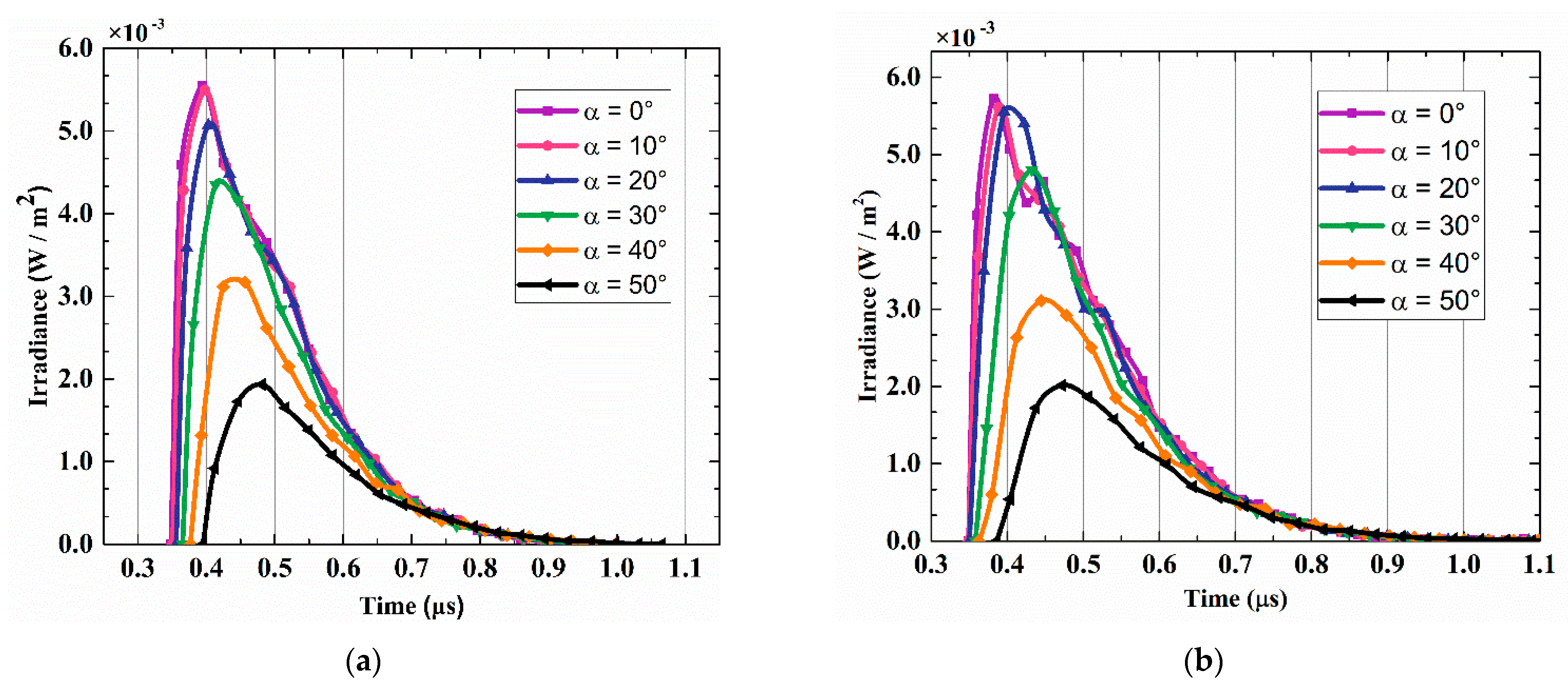
In general, when the distance r is a constant, there is a time delay of the received scattering light signal. Different off-axis angles α will lead to different signal delays in single-scattering mode, as shown in Figure 4a, Figure 5a, Figure 6a, Figure 7a, Figure 8a and Figure 9a. This is because as α increases, the non-coplanarity of the transceiver increases, and so does the shortest propagation range for a photon. The shortest propagation time of the received photons increases and it will let fewer photons be absorbed and scattered, and the peak of the received irradiance decreases.

In Figure 5a, when the light source is an LED with a Lambertian distribution, the received signals are also delayed. The difference is that the peak of the received irradiance has shifted to the right along the time line, and the received irradiance is much higher (nearly one order of magnitude) than that from the ordinary light source. This is because the light intensity of the LED is more concentrated in the paraxial region.

It also makes the light source more sensitive to non-coplanar deflection angles α. When α = 40°, the received irradiance is very weak and close to zero. When $\alpha ={50}^{°}$, photons simply cannot reach the receiver with only a single scattering in (Figure 5a). However, there are still some weak signals in multiple-scattered signals, as shown in Figure 5b.

For the Gaussian expanded laser beam, the curves of UV irradiance shown in Figure 6 behaved similarly to those of the LEDs in Figure 5, but there were differences specifically in the following two aspects. First, in Figure 6, the irradiance curve of the expanded laser beam is always located below the LED. Second, in Figure 6, when α = 0°, 10°, 20°, the peak value of the expanded laser is lower than the LED’s in Figure 5, but when α = 30°, 40°, 50°, the situation is reversed. This shows that the irradiance of the detector is not only related to the non-coplanarity of the transceiver, but also to the light intensity distribution of the light source.

In Figure 9a,b, the other variables were kept the same and the light source was replaced with an unexpanded Gaussian beam (${\varphi }_{\mathrm{T}}=0.01\mathrm{rad}$), In Figure 9a, the received signals became more sensitive to α. When α ≥ 30°, we could not detect the signals in single-scattering mode. We could still detect weak signals in multiple-scattering mode under this circumstance.

Under the single-scattering mode, the common scattering volume formed by the thin laser beam and the receiving FOV was very small, which resulted in a very limited time-span of photon propagation. Under the multiple-scattering mode, the curve in Figure 9b did not change much, but the detector captured trace photons outside the original time range.

For application in short-range detection instead of long-distance optical communications, we simulated the received signal a short distance from the transceivers.

In Figure 7 and Figure 8, compared to Figure 4, Figure 5, Figure 6 and Figure 9, the peaks of the curves were increased by two to three orders of magnitude. The pulse width was reduced by an order of magnitude (in Figure 7a, the pulse time ranged from 0.03 μs to 0.16 μs.) In the case of short-distance transmission, the off-axis angle $\alpha$ had little effect on the irradiance. As can be seen from Figure 7a, even when $\alpha ={50}^{°}$, the peak value dropped from only $2.25W/m^2$ to $1.75W/m^2$.

4. Analysis of the Received Energy Density

We also simulated the relationship between the energy received by the receiver under different types of light sources and the distance of transmission and reception. The output energy of the light was assumed to be 1mJ and the detector had a diameter $d$ of 1.5 cm. During the simulation, $N={10}^6$ photons were simulated and the received energy density of the detector can be expressed as

$$E_R=\frac{E_0}{N\pi {\left(d/2\right)}^2}{\displaystyle \sum _{i=1}^N{P}_{ni}},$$

(15)

where $E_0$ represents the total initial energy of the light source. $P_{ni}$ refers to the total received probability of the ith photon.

The test results are shown in Figure 10. Overall, no matter what kind of light source, the energy density of the received signal $E_{\mathrm{R}}$ decreased sharply with the increase of the sending and receiving distance.

As shown in Figure 10, light sources with different illuminating properties had different rates of acceptance energy reduction.

Comparing the two curves of Laser beams 1 and 2 in Figure 10a,b, for received energy density $E_R$, within a certain distance of $r$ in Figure 1, we can see that a smaller transmitting light convergence ${\varphi }_T$ was more favorable to improve the receiving energy when the laser transmitting energy $E_0$ and the elevation angle ${\theta }_T$, ${\theta }_R$ remained unchanged.

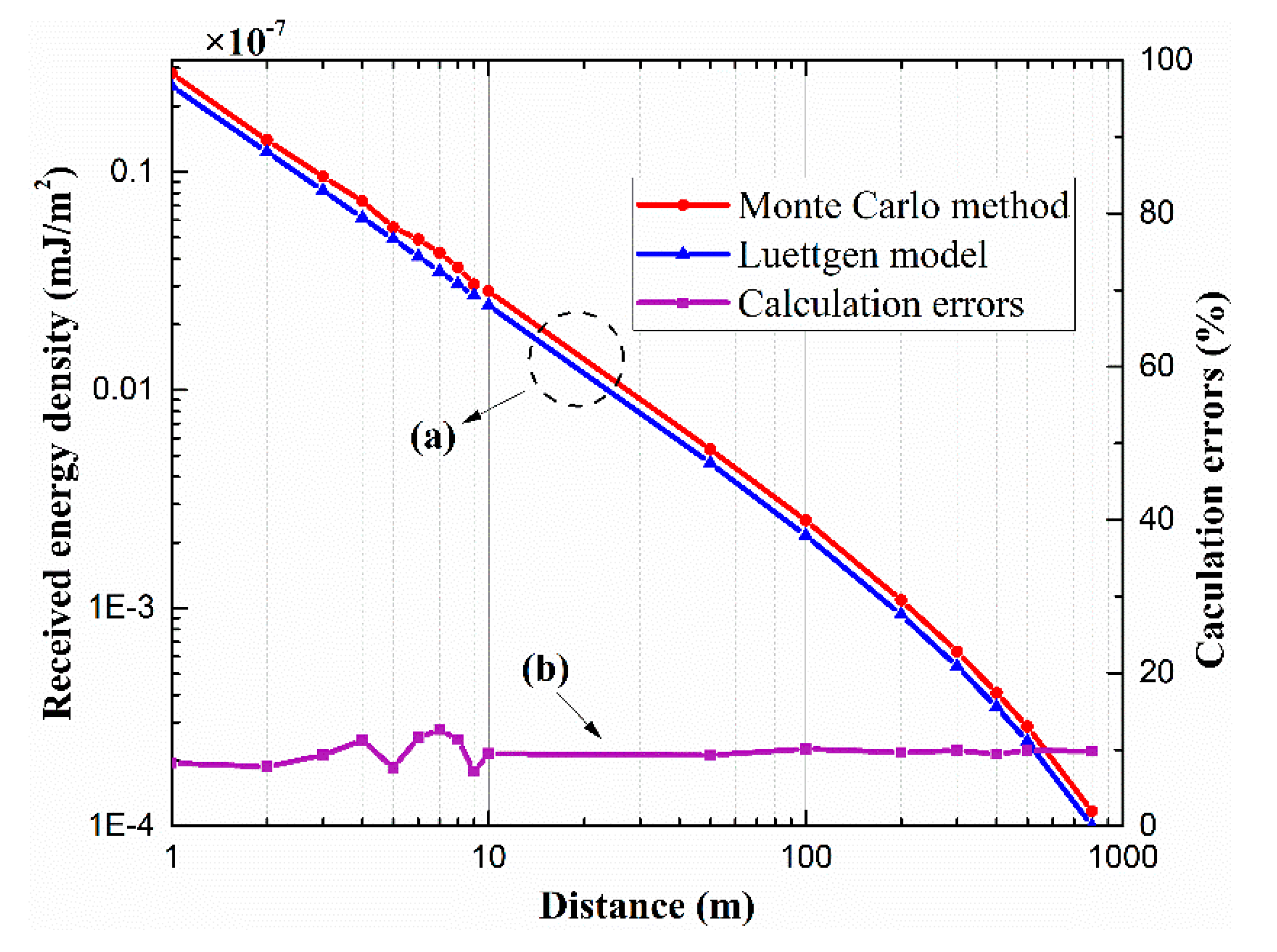
To verify the correctness of the program above, we compared the results with data obtained using the Luettgen classic model [6]. The relationships between received energy density $E_J$ and distance r are shown in Figure 11a on the left Y axis. The numerical differences $\left(E_{J,MC}-E_{J,Luettgen}\right)$ are shown in

Table 2. The numerical differences of Figure 11 ($E_{J,}{}_{MC}-E_{J,Luettgen}$ ).

Distances r	${\mathit{E}}_{\mathit{J},}{}_{\mathit{M}\mathit{C}}-{\mathit{E}}_{\mathit{J},\mathit{L}\mathit{u}\mathit{e}\mathit{t}\mathit{t}\mathit{g}\mathit{e}\mathit{n}}$
1	$2.15 \times {10}^{-9}$
2	$1.01 \times {10}^{-9}$
3	$8.10 \times {10}^{-10}$
4	$7.41 \times {10}^{-10}$
5	$3.93 \times {10}^{-10}$
6	$5.09 \times {10}^{-10}$
7	$4.77 \times {10}^{-10}$
8	$3.72 \times {10}^{-10}$
9	$2.04 \times {10}^{-10}$
10	$2.46 \times {10}^{-10}$
50	$4.53 \times {10}^{-11}$
100	$2.31 \times {10}^{-11}$
200	$9.54 \times {10}^{-12}$
300	$5.70 \times {10}^{-12}$
400	$3.51 \times {10}^{-12}$
500	$2.58 \times {10}^{-12}$
800	$1.04 \times {10}^{-12}$

. For the sake of simplicity, we only tested ordinary light sources under the single-scattering model. Since only the molecular scattering coefficient was considered in Luettgen’s paper, we ignored the effects of aerosols in the following test. The specific parameter settings are shown in Figure 11, and the calculation errors $\left(E_{J,MC}-E_{J,Luettgen}\right){/E}_{J,Luettgen}$ are shown in Figure 11 on the right Y axis.

It can be seen that the results obtained by the two models were similar. The trends of the curves were roughly the same. The differences between the two curves were chiefly caused by the randomness of the Monte Carlo point probability model and the two different ways of curve fitting.

5. Conclusions

In conclusion, a model of UV light atmospheric transport under different types of light source based on a Monte Carlo point probability method is presented. The results indicated that due to the different optical density distributions, under the single-scattering model or multiple scattering, different types of light sources will affect the distribution of the received signal, which includes irradiance and time offset of the pulse peak. In the case of single scattering, the degree of misalignment of the transceiver $\alpha$ affects the peak and width of the received pulse. When $\alpha$ increases, a wider pulse width and smaller peak value can be obtained. For different light sources, in the case of the same divergence angle, the peak value of the received signal will be different due to the different energy density distributions of the different lights. Multiple scattering will cause a time broadening of the received optical pulse, but it does not bring much improvement to the received energy density. Regardless of the source, the energy density received by the detector decreases exponentially as the distance from the transceiver increases, but the rate of decrease is different. Based on these simulation data, an appropriate light source can be selected according to the actual needs, and the gate-controlled switch of the detector can be controlled according to the impulse response. We hope our research will offer good technical support for short-range ultraviolet atmospheric communication and ultraviolet detection.

References

- Zhang, S.; Wang, J.; Xu, Z.; Chao, S.; Rong, W.; Chen, Y.; Zhao, J.; Wei, Y. Attenuation analysis of long-haul nlos atmospheric optical scattering communication. Opt. Laser Technol. 2016, 80, 51–55. [Google Scholar] [CrossRef]
- Sun, X.J.; Li, S.H.; Yan, W.X.; Zhang, R.W.; Zhang, C.L. Non-line-of-sight optical scattering communication based on atmospheric inhomogeneity. Opt. Commun. 2017, 382, 318–323. [Google Scholar] [CrossRef]
- Vavoulas, A.; Sandalidis, H.G.; Chatzidiamantis, N.D.; Xu, Z.; Karagiannidis, G.K. A Survey on Ultraviolet C-Band (UV-C) Communications. IEEE Commun. Surv. Tutor. 2019, 21, 2111–2133. [Google Scholar] [CrossRef]
- Reitebuch, O.; Lemmerz, C.; Nagel, E.; Paffrath, U.; Durand, Y.; Endemann, M.; Fabre, F.; Chaloupy, M. The airborne demonstrator for the direct-detection doppler wind lidar aladin on adm-aeolus. part i: Instrument design and com-parison to satellite instrument. J. Atmos. Ocean. Technol. 2009, 26, 2501–2515. [Google Scholar] [CrossRef] [Green Version]
- Lavigne, C.; Durand, G.; Roblin, A. Ultraviolet light propagation under low visibility atmospheric conditions and its application to aircraft landing aid. Appl. Opt. 2006, 45, 9140–9150. [Google Scholar] [CrossRef] [PubMed]
- Shen, F.; Zhuang, P.; Shi, W.; Qiu, C.; Wang, B.; Xie, C. Fabry–perot etalon-based ultraviolet high-spectral-resolution lidar for tropospheric temperature and aerosol measurement. Appl. Phys. B 2018, 124, 138. [Google Scholar] [CrossRef]
- Gong, C.; Wang, K.; Xu, Z.; Wang, X. On full-duplex relaying for optical wireless scattering communication with on-off keying modulation. IEEE Trans. Wirel. Commun. 2018, 17, 2525–2538. [Google Scholar] [CrossRef]
- Fountoulakis, I.; Natsis, A.; Siomos, N.; Drosoglou, T.; Bais, A.F. Deriving aerosol absorption properties from solar ultraviolet radiation spectral measurements at Thessaloniki, Greece. Remote Sens. 2019, 11, 2179. [Google Scholar] [CrossRef] [Green Version]
- Raptis, I.P.; Kazadzis, S.; Eleftheratos, K.; Amiridis, V.; Fountoulakis, I. Single Scattering Albedo’s Spectral Dependence Effect on UV Irradiance. Atmosphere 2018, 9, 364. [Google Scholar] [CrossRef] [Green Version]
- Moosmüller, H.; Engelbrecht, J.P.; Skiba, M.; Frey, G.; Chakrabarty, R.K.; Arnott, W.P. Single scattering albedo of fine mineral dust aerosols controlled by iron concentration. J. Geophys. Res. Atmos. 2012, 117. [Google Scholar]
- Mok, J.; Krotkov, N.A.; Torres, O.; Jethva, H.; Li, Z.; Kim, J.; Koo, J.H.; Go, S.; Irie, H.; Labow, G.; et al. Comparisons of spectral aerosol single scattering albedo in Seoul, South Korea. Atmos. Meas. Tech. 2018, 11, 2295–2311. [Google Scholar] [CrossRef] [Green Version]
- Kazadzis, S.; Kouremeti, N.; Amiridis, V.; Arola, A.; Gerasopoulos, E. Aerosol absorption retrieval at ultraviolet wavelengths in a complex environment. Atmos. Meas. Tech. Discuss. 2012, 5, 6991–7023. [Google Scholar] [CrossRef]
- Ialongo, I.; Buchard, V.; Brogniez, C.; Casale, G.R.; Siani, A.M. Aerosol Single Scattering Albedo retrieval in the UV range: An application to OMI satellite validation. Atmos. Chem. Phys. Discuss. 2009, 9, 19009–19033. [Google Scholar] [CrossRef]
- Arola, A.; Kazadzis, S.; Krotkov, N.; Bais, A.; Gröbner, J.; Herman, J.R. Assessment of TOMS UV bias due to absorbing aerosols. J. Geophys. Res. Atmos. 2005, 110. [Google Scholar] [CrossRef] [Green Version]
- Drost, R.J.; Sadler, B.M. Survey of ultraviolet non-line-of-sight communications. Semicond. Sci. Technol. 2014, 29, 084006. [Google Scholar] [CrossRef]
- Reilly, D.M. Atmospheric Optical Communications in the Middle Ultraviolet; Massachusetts Institute of Technology: Cambridge, MA, USA, 1976. [Google Scholar]
- Luettgen, M.R.; Reilly, D.M.; Shapiro, J.H. Non-line-of-sight single-scatter propagation model. J. Opt. Soc. Am. A 1991, 8, 1964–1972. [Google Scholar] [CrossRef]
- Xu, Z.; Ding, H.; Sadler, B.M.; Chen, G. Analytical performance study of solar blind non-line-of-sight ultraviolet short-range communication links. Opt. Lett. 2008, 33, 1860–1862. [Google Scholar] [CrossRef]
- Song, P.; Liu, C.; Zhao, T.; Guo, H.; Chen, J. Research on pulse response characteristics of wireless ultraviolet communication in mobile scene. Opt. Express 2019, 27, 10670–10683. [Google Scholar] [CrossRef]
- Wang, L.; Xu, Z.; Sadler, B.M. Non-line-of-sight ultraviolet link loss in noncoplanar geometry. Opt. Lett. 2010, 35, 1263–1265. [Google Scholar] [CrossRef]
- Elshimy, M.A.; Hranilovic, S. Non-line-of-sight single-scatter propagation model for noncoplanar geometries. J. Opt. Soc. Am. Opt. Image Sci. Vis. 2011, 28, 420. [Google Scholar] [CrossRef]
- Wang, P.; Xu, Z. Characteristics of ultraviolet scattering and turbulent channels. Opt. Lett. 2013, 38, 2773. [Google Scholar] [CrossRef]
- Hutt, D.L.; Tofsted, D.H. Effect of atmospheric turbulence on propagation of ultraviolet radiation. Opt. Laser Technol. 2000, 32, 39–48. [Google Scholar] [CrossRef]
- Luo, P.; Zhang, M.; Han, D.; Li, Q. Performance analysis of short-range nlos uv communication system using monte carlo simulation based on measured channel parameters. Opt. Express 2012, 20, 23489–23501. [Google Scholar] [CrossRef] [PubMed]
- Chen, G.; Xu, Z.; Sadler, B.M. Experimental demonstration of ultraviolet pulse broadening in short-range non-line-of-sight communication channels. Opt. Express 2010, 18, 10500–10509. [Google Scholar] [CrossRef]
- Chen, G.; Xu, Z.; Ding, H.; Sadler, B.M. Path loss modeling and performance trade-off study for short-range non-line-of-sight ultraviolet communications. Opt. Express 2009, 17, 3929. [Google Scholar] [CrossRef] [PubMed]
- Raptis, N.; Pikasis, E.; Syvridis, D. Power losses in diffuse ultraviolet optical communications channels. Opt. Lett. 2016, 41, 4421–4424. [Google Scholar] [CrossRef]
- Qin, H.; Zuo, Y.; Li, F.; Cong, R.; Meng, L.; Wu, J.; Qin, H.; Zuo, Y.; Li, F.; Cong, R. Analytical link bandwidth model based square array reception for non-line-of-sight ultraviolet communication. Opt. Express 2017, 25, 22693. [Google Scholar] [CrossRef]
- Fan, X.; Zheng, W.; Singh, D.J. Light scattering and surface plasmons on small spherical particles. Light Sci. Appl. 2014, 3, e179. [Google Scholar] [CrossRef] [Green Version]
- Xunli, X.; Binhai, Y.; Zhenqiang, M. Design on Approximate Lambertian LED Opto Lens Configuration. Electro-Opt. Technol. Appl. 2010, 25, 22–37. [Google Scholar]
- Wu, D.; Ghassemlooy, Z.; Le Minh, H.; Rajbhandari, S.; Khalighi, M.A.; Tang, X. Optimisation of Lambertian order for indoor non-directed optical wireless communication. In Proceedings of the 2012 1st IEEE International Conference on Communications in China Workshops (ICCC), Bejing, China, 15–17 August 2012; pp. 43–48. [Google Scholar]
- Milsom, P.K. A ray-optic, Monte Carlo, description of a Gaussian beam waist–applied to reverse saturable absorption. Appl. Phys. B 2000, 70, 593–599. [Google Scholar] [CrossRef]
- Arnaud, J.A.; Hubbard, W.M.; Mandeville, G.D.; De la Claviere, B.; Franke, E.A.; Franke, J.M. Technique for fast measurement of Gaussian laser beam parameters. Appl. Opt. 1971, 10, 2775–2776. [Google Scholar] [CrossRef] [PubMed]
- Bucholtz, A. Rayleigh-scattering calculations for the terrestrial atmosphere. Appl. Opt. 1995, 34, 2765–2773. [Google Scholar] [CrossRef] [PubMed]
- Zachor, A.S. Aureole radiance field about a source in a scattering absorbing medium. Appl. Opt. 1978, 17, 1911. [Google Scholar] [CrossRef] [PubMed]
- Shaw, G.A.; Nischan, M.L.; Iyengar, M.A.; Kaushik, S.; Griffin, M.K. NLOS UV communication for distributed sensor systems. Integr. Command Environ. 2000, 4126, 83–96. [Google Scholar]
- Ding, H.; Chen, G.; Majumdar, A.K.; Sadler, B.M.; Xu, Z. Modeling of non-line-of-sight ultraviolet scattering channels for communication. IEEE J. Sel. Areas Commun. 2009, 27, 1535–1544. [Google Scholar] [CrossRef]
- Chen, G.; Abou-Galala, F.; Xu, Z.; Sadler, B.M. Experimental evaluation of LED-based solar blind NLOS communication links. Opt. Express 2008, 16, 15059–15068. [Google Scholar] [CrossRef]
Figure 1.
The ultraviolet light atmospheric transmission model.
Figure 2.
(a) Plot of the LED’s normalized light intensity contrast as a function of off-axis angle . (b) vs. curve drawn by Mathematica.
Figure 3.
Plot of the different light sources’ normalized light intensity vs. off-axis angle .
Figure 4.
Curves of the UV irradiance vs. time with an ordinary light source under single scattering (SS) (a) and multiple scattering (MS) (b) modes.
Figure 5.
Curves of the UV irradiance vs. time with a Lambertian LED light source under SS (a) and MS (b) modes.
Figure 6.
Curves of the UV irradiance vs. time with a Gaussian expanded laser beam under SS (a) and MS (b) modes.
Figure 7.
Curves of the UV irradiance vs. time with Gaussian laser beam 1 under SS (a) and MS (b) modes.
Figure 8.
Curves of the UV irradiance vs. time with Gaussian laser beam 2 under SS (a) and MS (b) modes.
Figure 9.
Curves of the UV irradiance vs. time with Gaussian laser beam 3 under SS (a) and MS (b) modes.
Figure 10.
Curves of the received energy density vs. distance r under different light sources by single scattering. Parameters of the light sources are the same as in Figure 4, Figure 5, Figure 6, Figure 7, Figure 8 and Figure 9. (a) The linear scale in Y axis. (b)The log10 scale in Y axis.
Figure 11.
(a) Curves of the received energy density vs. distance . (b) The calculation errors of these two models. (, , λ = 266 nm, , , , single scattering, uniform light source.).