Development of Visible/Near-Infrared Hyperspectral Imaging for the Prediction of Total Arsenic Concentration in Soil

Abstract

Soil total arsenic (TAs) contamination caused by human activities—such as mining, smelting, and agriculture—is a problem of global concern. Visible/near-infrared (VNIR), X-ray fluorescence spectroscopy (XRF), and laser-induced breakdown spectroscopy (LIBS) do not need too much sample preparation and utilization of chemicals to evaluate total arsenic (TAs) concentration in soil. VNIR with hyperspectral imaging has the potential to predict TAs concentration in soil. In this study, 59 soil samples were collected from the Daye City mining area of China, and hyperspectral imaging of the soil samples was undertaken using a visible/near-infrared hyperspectral imaging system (wavelength range 470–900 nm). Spectral preprocessing included standard normal variate (SNV) transformation, multivariate scatter correction (MSC), first derivative (FD) preprocessing, and second derivative (SD) preprocessing. Characteristic bands were then identified based on Spearman’s rank correlation coefficients. Four regression models were used for the modeling prediction: partial least squares regression (PLSR) (R² = 0.71, RMSE = 0.48), support vector machine regression (SVMR) (R² = 0.78, RMSE = 0.42), random forest (RF) (R² = 0.78, RMSE = 0.42), and extremely randomized trees regression (ETR) (R² = 0.81, RMSE = 0.38). The prediction results were compared with the results of atomic fluorescence spectrometry methods. In the prediction results of the models, the accuracy of ETR using FD preprocessing was the highest. The results confirmed that hyperspectral imaging combined with Spearman’s rank correlation with machine learning models can be used to estimate soil TAs content.

1. Introduction

Arsenic (As) is a ubiquitous element in nature, and can be found in rocks, soils, sediments, fossil fuels, plants, and almost all living organisms, including the biota of aquatic ecosystems [1]. Worldwide total arsenic (TAs) levels in soils have been reported to range between 2 and 5 mg/kg [2,3]. However, TAs can be very harmful due to excessive accumulation in agricultural soils [4,5]. Firstly, the transfer of TAs from soil to human beings through the food chain poses a potential disease risk [6,7]. Secondly, excess TAs entering the pedosphere can affect the quality of cultivated land and reduce productivity [7,8]. Research has suggested that the TAs can be accumulated due to human activities such as mining and smelting, industrial processes, and agricultural fertilizers. Most countries have been confronted with the soil contamination caused by heavy metals has become a worldwide issue [9,10,11,12,13]. Traditional chemical-based methods are destructive, time-consuming, and expensive. Therefore, nondestructive, cheap, and rapid methods for detecting soil TAs content, such as hyperspectral imaging, are needed to avoid human health risks and achieve soil protection [14].

Visible/near infrared (VNIR), X-ray fluorescence spectroscopy (XRF), and laser-induced breakdown spectroscopy (LIBS) do not need too much sample preparation and utilization of chemicals to evaluate TAs concentration in soil [15,16]. Hyperspectral imaging utilizes the VNIR spectrum and is used under laboratory conditions to acquire high spectral resolution images of soil, through its advantages of being fast, effective, non-destructive, and low cost [17,18]. Prediction of TAs content is made possible by correlating the spectral data extracted from the hyperspectral images to their corresponding chemical concentrations [19]. Previous studies showed that the partial least squares (PLS) model can be used to determine the TAs concentration in soil samples (R²_p = 0.75, RMSE_p = 153.77) [20].

In recent years, the development of machine learning algorithms also allowed their application for the prediction of element concentration in soil by the use of hyperspectral imaging (400–2500 nm) [21,22,23]. Compared with support vector machine regression (SVMR), the random forest (RF) model is a more effective machine learning method for developing diagnosis models [23]. Feature selection and machine learning methods are now important methods of predicting total nitrogen, total zinc, and total magnesium [24,25]. Selecting the sensitive bands based on Spearman’s rank correlation coefficients is a common approach when estimating soil concentration content [24,25], but there is only a limited number of studies regarding the estimation of TAs content in soil using hyperspectral imaging technology. In addition, distribution maps obtained using hyperspectral imaging techniques are now widely used in agricultural studies, forestry, meat quality testing, etc. [26,27,28,29]. Meanwhile, the use of hyperspectral imaging techniques for generating soil TAs concentration distribution maps using machine learning models remains to be studied [30].

The objectives of this study were to investigate the use of VNIR hyperspectral imaging technology in the prediction of TAs concentration in soil. Preprocessing methods were used for selecting the characteristic bands in hyperspectral imaging technology, based on Spearman’s rank correlation coefficients. We also compared the machine learning techniques of PLSR, SVMR, RF, and extremely randomized trees regression (ETR) in the prediction of TAs concentration in soil. The estimation of soil TAs content was then achieved based on the best-performing regression model for the prediction of soil TAs concentration distribution map.

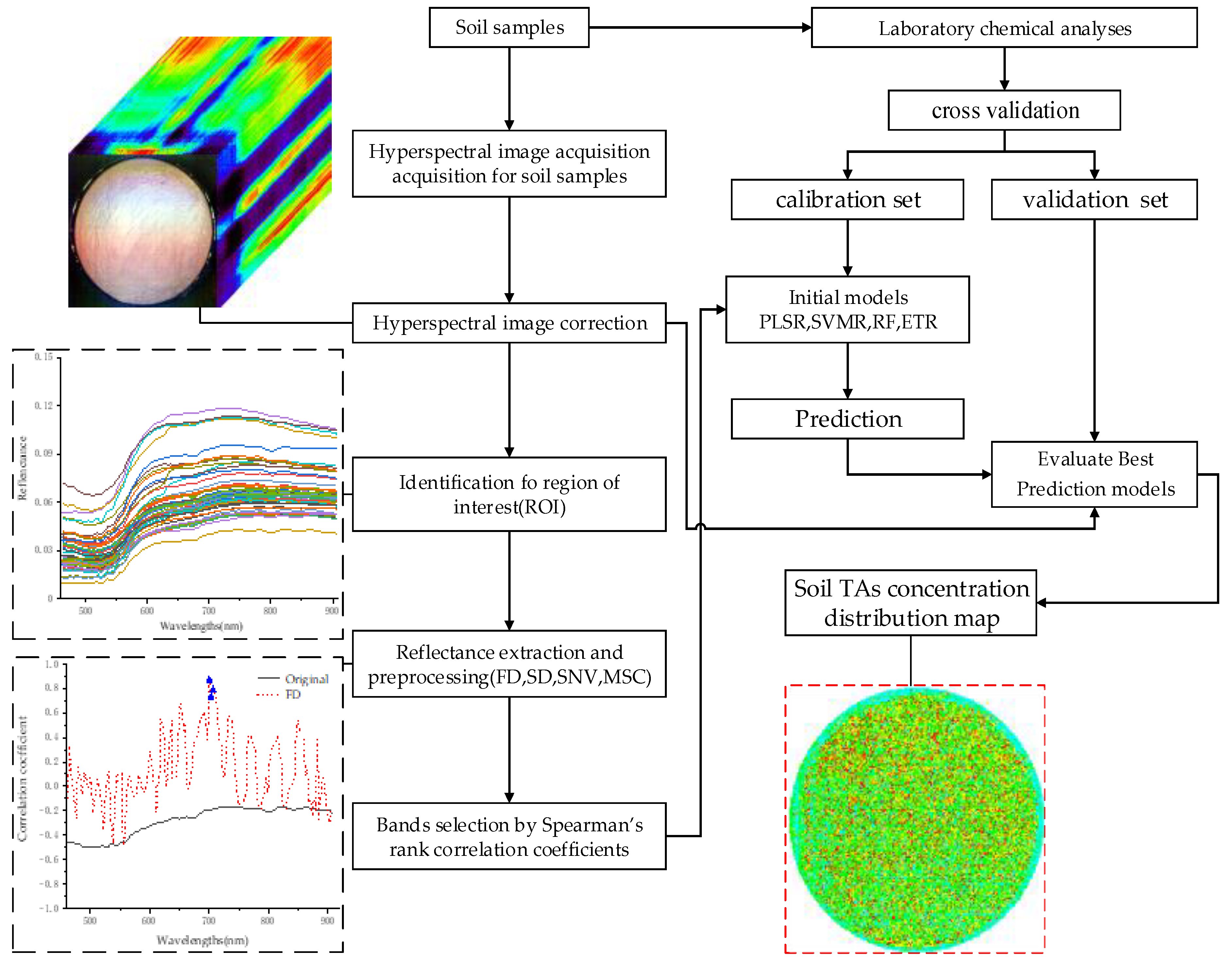
2. Materials and Methods

2.1. Sample Preparation and Soil Chemical Analysis

Soil samples used in this experiment were collected from the area of Daye mine, a typical area of Jianghan Plain in Hubei province, China (114°31′~115°20′E, 29°40′~30°40′N). The climate of this area is subtropical with an annual average temperature of 16.9 °C.According to the classification and codes for Chinese soil (National Standard of China, GB/T 17296-2009), the soils in this area are mainly red soil and yellow-brown soil. The Daye area is a production base of crops and rich in mineral resources [31]. The mining has greatly damaged the ecological environment, and the farmland soil near the mining area has been seriously polluted.

A total of 59 soil samples were collected from different types of cultivated soils near mining areas in Daye. They were taken from the upper soil layer (0–20 cm) in 2018. After removal of the stones and plant roots, then they were sifted through a 200-mesh sieve and then ground into fine particles, approximate particle size after grinding ≤74 µm [32]. Each soil sample was then divided into two parts. One part was sent to the laboratory digested with nitric acid/hydrochloric acid/perchloric acid. After that, measured by atomic fluorescence spectrometry (AFS) (AFS-9730, Haiguang, China) (National Standard of China: analysis of total arsenic contents in soils, GB/T 21191-2007, GB/T 22105.2-2008). Instrument limits of detection (LODs, mg/kg) were 0.001 for TAs. The other part was sent to the dark chamber for hyperspectral imaging (HSI) measurement. The highest observed soil TAs content was 16.41 µg/g and lowest was 7.04 µg/g. The averaged TAs content of soils average was 9.65 µg/g. The soil sample concentrations are listed in

Table 1. Statistical descriptions for the arsenic content (µg/g) and the soil sample percentages.

TAs	No.	Maximum	Minimum	Mean	Std.	Skewness	Kurtosis	Per%
Total data set	59	16.41	7.04	9.6527	1.4699	1.74	5.71	100

.

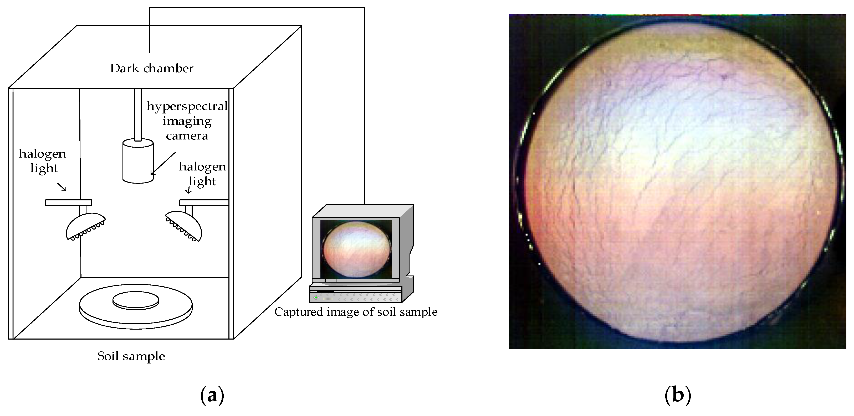
2.2. Hyperspectral Imaging System and Image Acquisition

A VNIR hyperspectral imaging system was used to capture images of the soil samples [33,34,35,36] (Figure 1a). The system consisted of the following components: a SNAPSCAN hyperspectral imaging camera (Imec, Belgium), operating in the spectral range of 470–900 nm, with a spectral resolution of 3 nm, producing a total 147 spectral bands; two current-controlled wide spectrum quartz halogen lights; a sample station for scanning; a dark chamber; and data acquisition software (Imec snapscan acquisition, Imec Corp, Leuven, Belgium). Soil samples were positioned on a moving stage and moved into the camera’s field of view. Samples were shaken after capturing each image for homogenization, and the imaging was repeated until reproducible spectral signatures were obtained for consecutive images. The acquired imagery (R: 640 nm, G: 548 nm, B: 470 nm) is illustrated in Figure 1b.

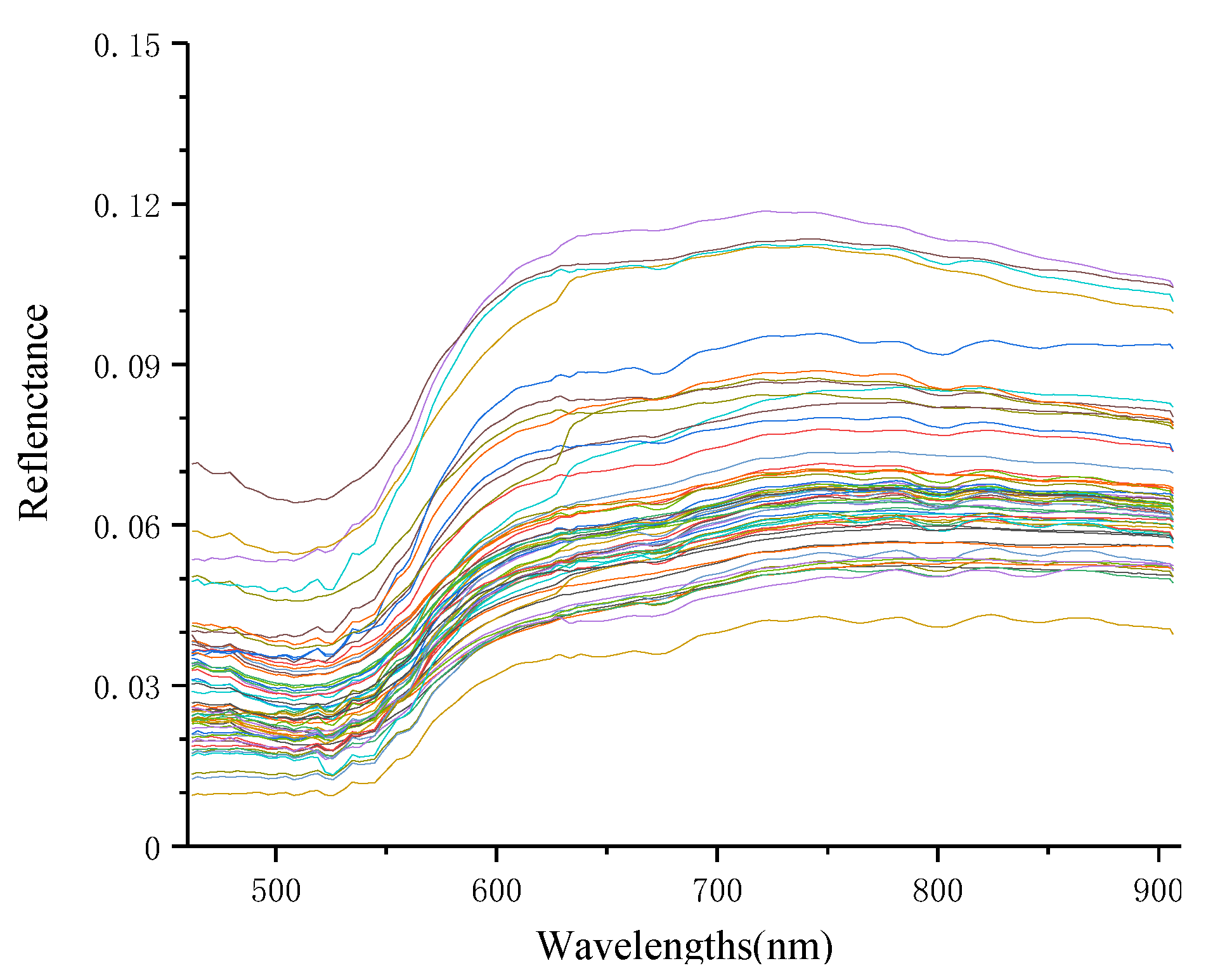
2.3. Spectral Profile Extraction and Data Calibration

To eliminate the impacts of uneven illumination and dark current noise, the raw hyperspectral imagery was calibrated by standard white and dark reference images according to the formula [37]

$$R_c=\frac{R_0-B}{W-B}$$

(1)

where R₀ indicates the raw hyperspectral image, R_c represents the calibrated hyperspectral image, W represents the standard white reference image obtained using a rectangular Teflon plate, and B denotes the standard black reference image obtained by covering the lens completely with an opaque black cover [38].

For each hyperspectral image, a region of interest (ROI) was used to measure the mean VNIR spectral reflectance. The ROI (a circle with a diameter of about 150 pixels) was positioned in the middle of the sample image, and close to Petri dish (90 × 17 mm) edge [20,39] (Figure 2). The spectral bands for this study are 519, 560, 564, 576, 697, 700, 703, 706, and 749 nm. The standard deviation of the averaged spectral band of each sample is between 30~50. The standard deviation of the 697 nm band is even lower than 20.

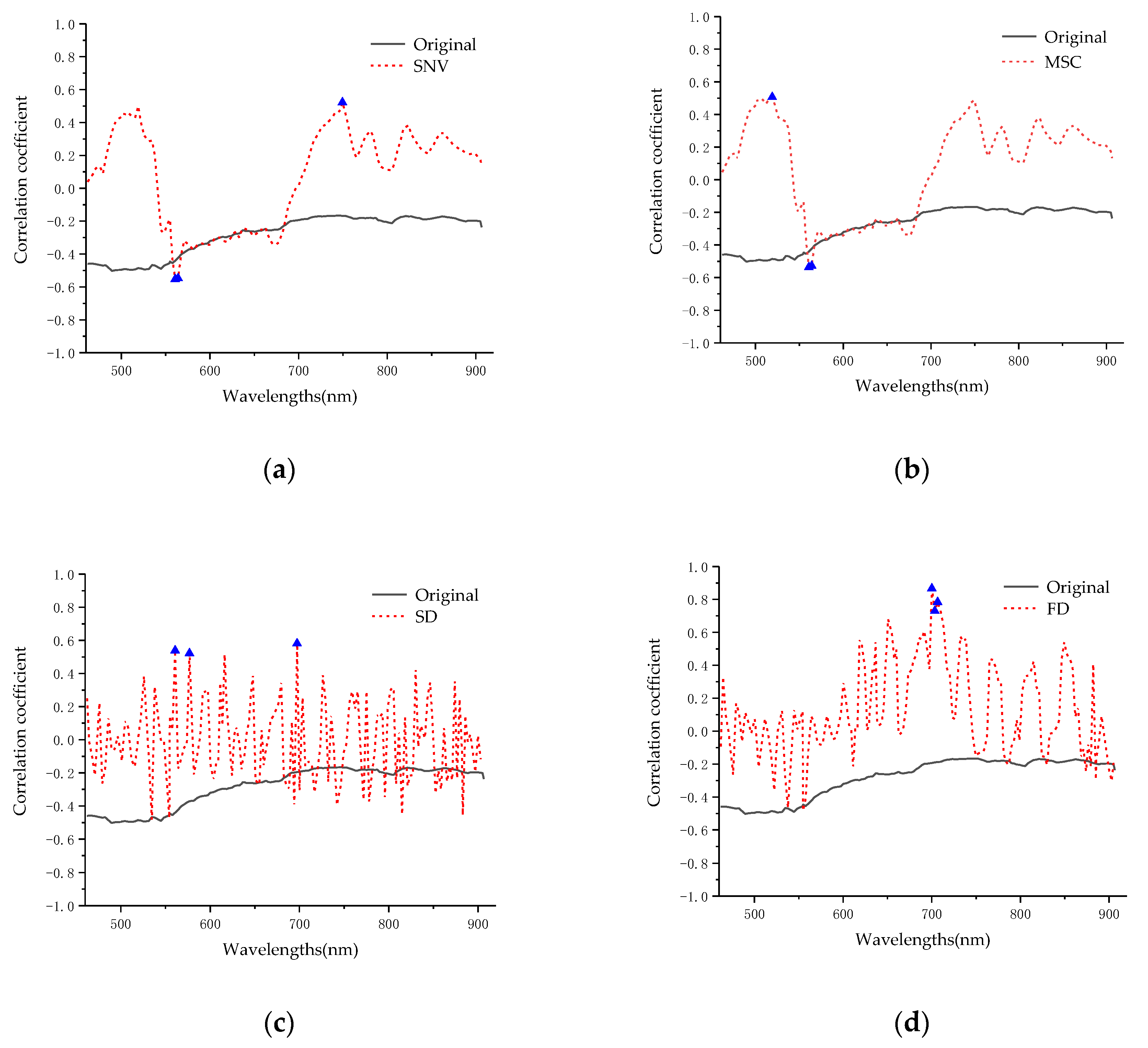
2.4. Feature Band Selection

The reflectance spectral data also contained other irrelevant information and noise. Therefore, before the establishment of the regression model, it was necessary to complete a basic preprocessing to remove the irrelevant information and noise. The common preprocessing methods are first derivative (FD) preprocessing, second derivative (SD) preprocessing, standard normal variate (SNV) transformation, and multivariate scatter correction (MSC) [18,40,41]. We then selected the bands with higher correlation according to the Spearman’s rank correlation coefficients [42].

2.5. Model Development and Evaluation

In this study, we refer to the detailed of the model information of previous studies, partial least squares regression (PLSR), support vector machine regression (SVMR), random forest (RF), and extremely randomized trees regression (ETR) models were used to analyze the soil sample data. Good results have been obtained in the past based on the PSLR model [20]. SVMR has been proven to be effective in predicting the TAs concentration in soil in many studies [43]. There are many methods for tuning the hyper-parameters of SVMR, grid search being the most frequently used. In this study, use as grid search computes performance at all pairs of e and C to get the performance surface [44]. RF has been reported as performing better than PLSR and SVMR [23,45].

In addition, we also considered the ETR model developed in recent years on the basis of the RF model. The ETR model has been reported as having a higher prediction accuracy than the RF model for soil elements, and has been used in soil spectral prediction models in recent years [46]. ETR was developed as an extension of another tree-based ensemble method (random forest) to be a more computationally efficient algorithm. It consists of three factors: K is the number of randomly selected variables for splitting a node, n_min represents the minimum number of samples required for splitting an internal node, and M, the number of trees formed in the ensemble model [47].

According to the results of laboratory measurement samples, the 59 soil samples were divided using the 10-fold cross validation method into calibration set and validation set [48].

The main steps of the work were shown in Figure 3. After hyper spectral image acquisition, correction and reflectance preprocessing, and the ROI spectrum was extractwed. Through the pretreatment methods of FD, SNV and MSC, combined with the Spearman’s rank correlation coefficients, the characteristic bands were selected, and the PLSR, SVMR, RF, and ETR models were compared. The best model was used to estimate the soil TAs content and generate the soil TAs distribution map.

The parameters of the determination coefficients (R²), root-mean-square error (RMSE), and relative error (RE%) were used to measure the accuracy of the models [39,49]. The closer R² is to 1, the better the stability of the model and the higher the degree of fit. RMSE and RE were used to test the predictive ability of the models. The smaller the RMSE and RE, the better the predictive ability.

$$R^2=1-\frac{{\displaystyle \sum _{n-1}^n{(y_i-{\widehat{y}}_i)}^2}}{{\displaystyle \sum _{n-1}^n{(y_i-{\overline{y}}_i)}^2}}$$

(2)

$$RMSE=\sqrt{\frac{{\displaystyle \sum _{n-1}^n{(y_i-{\widehat{y}}_i)}^2}}{n}}$$

(3)

$$RE=100\times \frac{RMSE}{\overline{y}}$$

(4)

where n is the number of samples, y_i is the measured value, $\widehat{y}$_i is the predicted value, and $\overline{y}$ is the average of the measured values.

3. Results and Discussion

3.1. Preprocessing Comparative Analysis

Feature selection can improve the prediction performance, and gain a better understanding of the data in machine learning. Feature selection by correlation is a commonly used feature selection method [24,25]. In this study, a Spearman’s rank correlation analysis between the TAs concentration in the soil and the preprocessed spectra was carried out.

The preprocessing of the soil spectral can effectively highlight the absorption and reflection bands [18,40,41]. We calculated the Spearman’s rank correlation coefficients for the spectral bands after FD, SD, SNV, and MSC preprocessing (Figure 4). In Figure 4, the black line is the original spectrum Spearman’s rank correlation coefficients, where it can be seen that the correlation is low, around −0.4 to 0.5. After SNV, MSC, and SD preprocessing, some bands have been improved (red line), but the correlation is still low (0.4 to 0.5). After FD preprocessing, we find bands with correlation of higher than 0.8 appears near the 700 nm region TAs previous studies indicated [20,23,33], the VIS-NIR (650–700 nm) included important wavelengths for estimating TAs contents in soil. Therefore, we selected the three bands (Blue triangle in Figure 4) with the highest correlation coefficient, around 700 nm, and input this into the different machine learning models for calculation. Meanwhile, the three bands (blue triangle in Figure 4) with the highest correlation coefficients in other preprocessing methods are selected for comparison [42].

We then used the model to predict the final result so that we could evaluate the model effect. The results are shown in

Table 2. Results of model regression based on the different preprocessing methods.

Preprocessing and Modeling	Characteristic Bands Wavelength (nm) and Correlation Coefficients	Validation
		${{\mathit{R}}^2}_{\mathbf{CV}}$	RMSECV	REcv(%)
SNV+PLSR	560.7 (−0.55), 564.0 (−0.54), 749.5 (0.52)	0.49	0.63	6.63
SNV+SVMR		0.56	0.58	6.14
SNV+RF		0.53	0.60	6.31
SNV+ETR		0.59	0.56	5.86
MSC+PLSR	519 (0.50), 560.7 (−0.53), 564.0 (−0.52)	0.07	0.76	7.88
MSC +SVMR		0.23	0.69	7.22
MSC +RF		0.25	0.68	7.15
MSC +ETR		0.26	0.67	6.98
SD+PLSR	560.7 (0.53), 576.7 (0.52), 697.0 (0.58)	0.23	0.64	6.64
SD +SVMR		0.36	0.58	6.09
SD +RF		0.51	0.51	5.47
SD +ETR		0.51	0.51	5.43
FD+PLSR	700 (0.86), 703 (0.72), 706 (0.78)	0.71	0.48	5.03
FD +SVMR		0.78	0.42	4.50
FD +RF		0.78	0.42	4.45
FD +ETR		0.81	0.38	4.08

. After using SNV, MSC, and SD preprocessing, three bands selected according to the correlation were input into the prediction models, and each model prediction set result was poor. However, the prediction effect of the model with high correlation (0.7 or higher) after using the FD preprocessing is ideal. This shows that as the correlation coefficient increases, the effect of the model increases. Using a higher correlation band can greatly improve the stability and predictability of the model [50]. Finally, FD was selected as the preprocessing method, and the three characteristic bands with the highest correlation (700, 703, and 706 nm) were selected for the modeling.

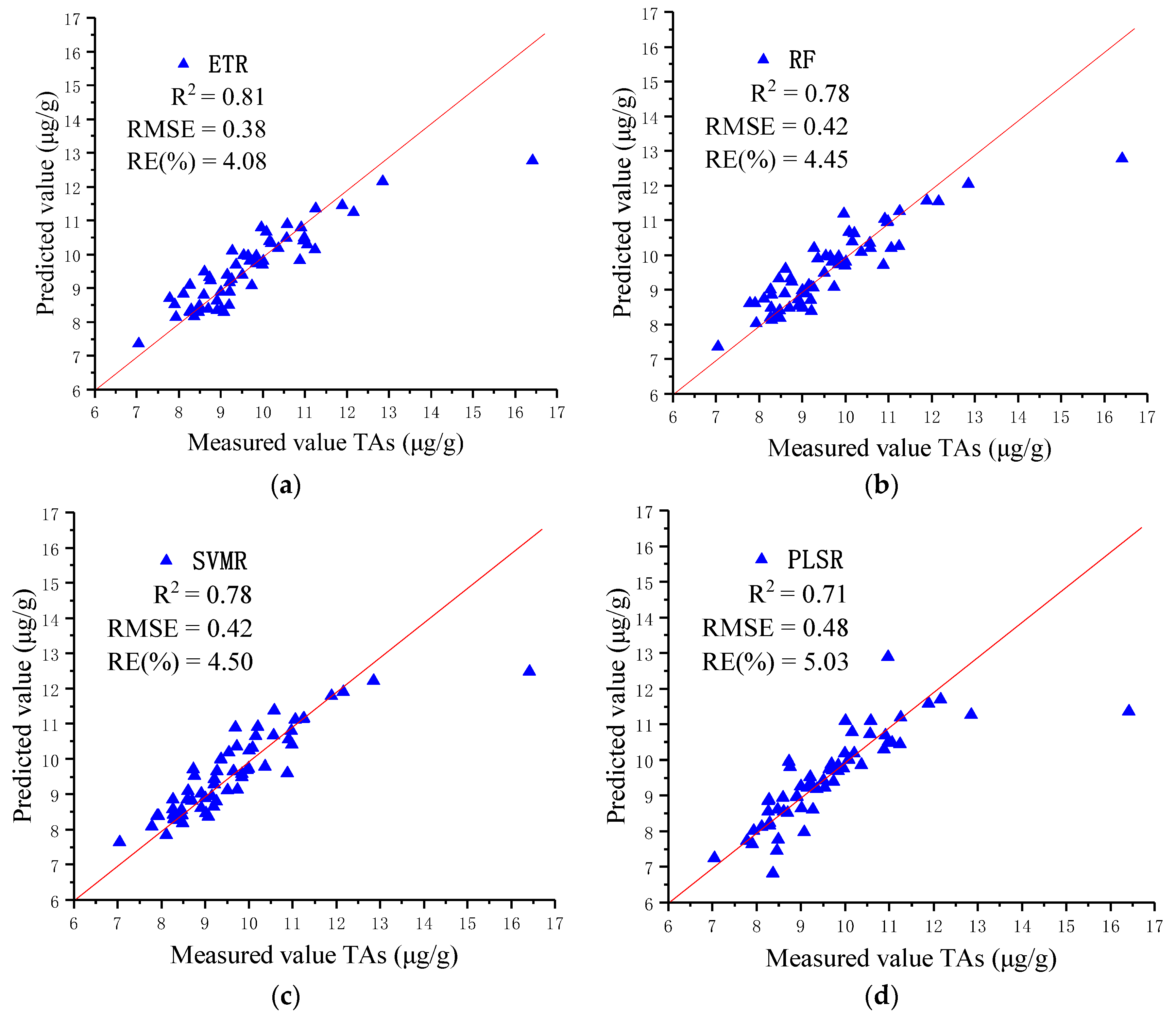
3.2. Regression Model

PLSR, SVMR, RF, and ETR were used to model the regression. The calibration set was used to train the prediction of the TAs concentration in the soil model. Comparing the model predictions with the validation sets, it can be seen from Figure 5 that the four models all obtain a good accuracy. Model predictive power is estimated by the R². The closer the value of R² to 1, and closer the scatter plot of the measured value and predicted accuracy value for the 1:1 line. Among them, the ETR regression model shows the smallest deviation from the 1:1 line, and the degree of fitting is the highest. Model predictive accuracy estimated by the RMSE and RE (%). Most of the predictions are closely distributed around the 1:1 line, few predictions far away from the 1:1 line generated errors, indicating that the models are accurate. From the results of the model accuracy evaluation, the RMSE of the ETR (RMSE = 0.38) model is the lowest, RE (%) of the ETR (RE = 4.08%) model is also lower, indicating that the ETR prediction accuracy is optimal.

From

Table 3. Accuracy validation of the different models.

Modeling Method	R2cv	RMSEcv	REcv (%)
PLSR	0.71	0.48	5.03
SVMR	0.78	0.42	4.50
RF	0.78	0.42	4.45
ETR	0.81	0.38	4.08

, it can be seen that the PLSR prediction is lowest, and the R², RMSE, and RE (%) of the validation set are 0.71, 0.48, and 5.03, respectively. Meanwhile, the R², RMSE, and RE (%) of the ETR validation set are 0.81, 0.38, and 4.08, respectively, which represent the best prediction results for prediction models. In summary, ETR has advantages in four models of model prediction power and prediction accuracy.

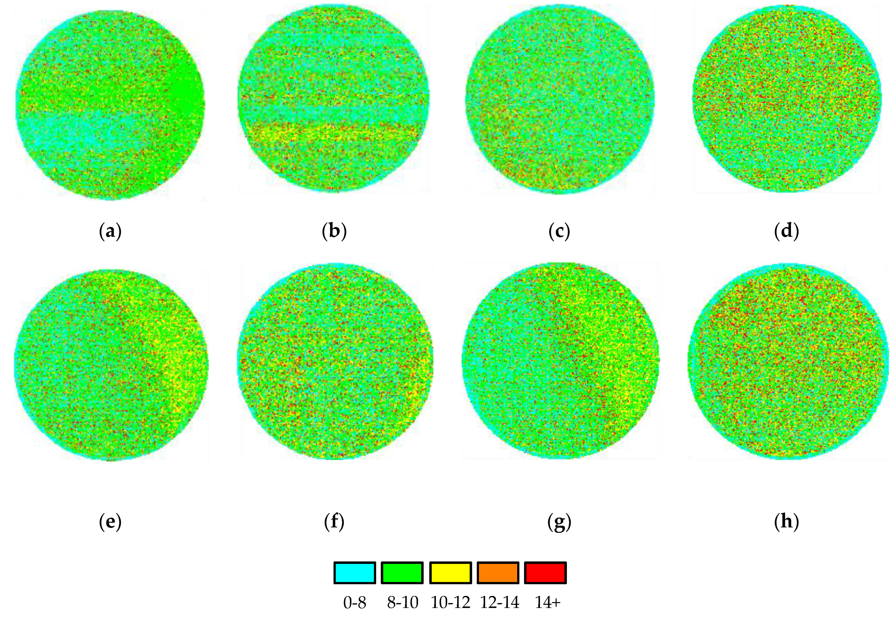
3.3. Concentration Distribution Map

The superiority of hyperspectral images to simultaneously obtain both spectral and spatial information makes it possible to display the results of soil TAs concentration distribution map. This study picks eight soil sample hyperspectral images to generate a TAs concentration distribution map, the maximum TAs concentration soil sample (Figure 6h), minimum TAs concentration soil sample (Figure 6a), and 6 other TAs soil samples. The best model—ETR based on FD preprocessed—was selected to visualize the soil TAs concentration distribution map. The spectral information on each pixel in hyperspectral images was input into ETR model to predict the results. Combined with the prediction results of spatial location information of hyperspectral images, the TAs concentration distribution map could be eventually formed [37,51]. Then, according to the prediction values, divide the values in the graph into five intervals to statistical analysis, cyan (0–8 µg/g), green (8–10 µg/g), yellow (10–12 µg/g), orange (12–14 µg/g), and red (14+ µg/g) (Figure 6).

In Figure 6, with more cyan and green sample distribution maps, the sample prediction value is low. Sample distribution maps with more red, orange, and yellow have higher predicted values. According to the results in the Figure 6, mean and standard deviation were statistically analyzed, as shown in

Table 4. Statistical summary of the TAs distribution maps.

No.	Measured Value (μg/g)	Std.	Mean	0–8 (μg/g)	8–10 (μg/g)	10–12 (μg/g)	12–14 (μg/g)	14+ (μg/g)
a	7.04	4.10	8.01	37%	42%	4%	13%	4%
b	8.26	4.12	8.58	32%	47%	5%	11%	5%
c	8.69	4.13	8.59	25%	56%	7%	8%	4%
d	9.36	4.20	8.63	23%	54%	5%	11%	7%
e	10.58	4.23	8.68	24%	50%	10%	9%	6%
f	11.05	4.36	8.92	23%	51%	9%	11%	6%
g	11.25	4.37	8.96	25%	48%	12%	10%	5%
h	16.41	4.39	9.05	22%	48%	9%	13%	8%

.

Shown in Table 4, all soil sample maps with low values (0–10) µg/g (cyan and green) totaled around 75%. The higher area (more than 10 µg/g) (yellow, orange, red) is about 25%. Meanwhile, according to Table 4, HSI predicted TAs and measured TAs used the standard deviation plotted as error bars for each sample is drawn (Figure 7).

As shown in Figure 7, the mean HSI predicted value increases as the measured value increases, confirming a positive correlation between the two datasets. Furthermore, on the whole, the HSI and measured values are in agreement when considering the standard deviation associated with the HSI prediction.

Overall, the results of TAs content in soil samples for measured value were compared with the results shown in the distribution map. The results show that the concentration gradually increases from soil sample a to soil sample h. This confirms that the model is highly correlated with the real results. It shows that the soil TAs content distribution map generated by the model is valid.

4. Conclusions

In this study, we collected 59 soil samples from the Daye City mining area of China. Hyperspectral imaging of the soil samples was undertaken using a hyperspectral imaging system (470–900 nm). Through the pretreatment methods of FD, SNV, and MSC, combined with the Spearman’s rank correlation coefficients, the characteristic bands were selected, and the PLSR, SVMR, RF, and ETR models were compared. The ETR model was used to estimate the soil TAs content and generate the soil TAs distribution map. The main conclusions are as follows:

(1)

Using the images acquired in the hyperspectral imaging system, bands selected according to different correlation coefficients are put into different models for prediction, it was found that the Spearman’s rank correlation coefficients were an effective way to select the characteristic bands of TAs content. ETR (R² = 0.81, RMSE = 0.38), RF (R² = 0.78, RMSE = 0.42), SVMR (R² = 0.78, RMSE = 0.42) models are capable of predicting total As content.

(2)

Soil TAs concentration distribution map shows, the Spearman’s rank correlation coefficients selected bands for ETR model, to predict the soil TAs distribution map generated by the pixel spectral of the hyperspectral image can be used as for estimation of TAs concentration in soil.

The restriction on estimating total As could be considered a limitation of this present study. This is because not all forms of As are soluble and thus toxic. Therefore, in the context of toxicity, future research should focus instead on predicting the concentration of bioavailable As.

References

1. Cullen, W.; Reimer, K. ChemInform Abstract: Arsenic Speciation in the Environment. ChemInform 1989, 20, 713–764. [Google Scholar] [CrossRef]
2. Wedepohl, K. The Composition of the Continental Crust. Geochim. Cosmochim. Acta 1995, 59, 1217–1232. [Google Scholar] [CrossRef]
3. Rudnick, R.; Gao, S. Composition of the Continental Crust. Treatise Geochem 3:1–64. Treatise Geochem. 2003, 3, 1–64. [Google Scholar]
4. Shi, T.Z.; Liu, H.Z.; Wang, J.J.; Chen, Y.Y.; Fei, T.; Wu, G.F. Monitoring Arsenic Contamination in Agricultural Soils with Reflectance Spectroscopy of Rice Plants. Environ. Sci. Technol. 2014, 48, 6264–6272. [Google Scholar] [CrossRef]
5. Shi, T.Z.; Chen, Y.Y.; Liu, Y.L.; Wu, G.F. Visible and near-infrared reflectance spectroscopy-An alternative for monitoring soil contamination by heavy metals. J. Hazard. Mater. 2014, 265, 166–176. [Google Scholar] [CrossRef]
6. Kabata-Pendias, A.; Pendias, H. Trace Elements in Soils and Plants, 3rd ed.; CRC Press: Boca Raton, FL, USA, 2001. [Google Scholar]
7. Kabata-Pendias, A.; Mukherjee, A.B. Trace Elements from Soil to Humans; Springer: Berlin, Germany, 2007. [Google Scholar]
8. Miano, T.; D’Orazio, V.; Zaccone, C. Trace elements and food safety. In PHEs, Environment and Human Health. Potentially Harmful Elements in the Environment and the Impact on Human Health; Springer: Berlin, Germany, 2014; Volume 9, pp. 339–370. [Google Scholar]
9. Yang, Q.Q.; Li, Z.Y.; Lu, X.N.; Duan, Q.N.; Huang, L.; Bi, J. A review of soil heavy metal pollution from industrial and agricultural regions in China: Pollution and risk assessment. Sci. Total Environ. 2018, 642, 690–700. [Google Scholar] [CrossRef]
10. Stazi, S.R.; Cassaniti, C.; Marabottini, R.; Giuffrida, F.; Leonard, C. Arsenic uptake and partitioning in grafted tomato plants. Hortic. Environ. Biotechnol. 2016, 57, 241–247. [Google Scholar] [CrossRef]
11. Choe, E.; van der Meer, F.; van Ruitenbeek, F.; van der Werff, H.; de Smeth, B.; Kim, K.-W. Mapping of heavy metal pollution in stream sediments using combined geochemistry, field spectroscopy, and hyperspectral remote sensing: A case study of the Rodalquilar mining area, SE Spain. Remote Sens. Environ. 2008, 112, 3222–3233. [Google Scholar] [CrossRef]
12. Mahar, A.; Wang, P.; Ali, A.; Awasthi, M.K.; Lahori, A.H.; Wang, Q.; Li, R.H.; Zhang, Z.Q. Challenges and opportunities in the phytoremediation of heavy metals contaminated soils: A review. Ecotoxicol. Environ. Saf. 2016, 126, 111–121. [Google Scholar] [CrossRef]
13. Jiang, X.L.; Zou, B.; Feng, H.H.; Tang, J.W.; Tu, Y.L.; Zhao, X.G. Spatial distribution mapping of Hg contamination in subclass agricultural soils using GIS enhanced multiple linear regression. J. Geochem. Explor. 2019, 196, 1–7. [Google Scholar] [CrossRef]
14. Tao, C.; Wang, Y.J.; Cui, W.B.; Zou, B.; Zou, Z.R.; Tu, Y.L. A transferable spectroscopic diagnosis model for predicting arsenic contamination in soil. Sci. Total Environ. 2019, 669, 964–972. [Google Scholar] [CrossRef]
15. Cheburkin, A.; Shotyk, W. An Energy-dispersive Miniprobe Multielement Analyzer (EMMA) for direct analysis of Pb and other trace elements in peats. Anal. Bioanal. Chem. 1996, 354, 688–691. [Google Scholar] [CrossRef] [PubMed]
16. Dell’Aglio, M.; Gaudiuso, R.; Senesi, G.S.; De Giacomo, A.; Zaccone, C.; Miano, T.M.; De Pascale, O. Monitoring of Cr, Cu, Pb, V and Zn in polluted soils by laser induced breakdown spectroscopy (LIBS). J. Environ. Monit. 2011, 13, 1422–1426. [Google Scholar] [CrossRef] [PubMed]
17. Malmir, M.; Tahmasbian, I.; Xu, Z.H.; Farrar, M.B.; Bai, S.H. Prediction of soil macro- and micro-elements in sieved and ground air-dried soils using laboratory-based hyperspectral imaging technique. Geoderma 2019, 340, 70–80. [Google Scholar] [CrossRef]
18. Manley, M. Near-infrared spectroscopy and hyperspectral imaging: Non-destructive analysis of biological materials. Chem. Soc. Rev. 2014, 43, 8200–8214. [Google Scholar] [CrossRef] [Green Version]
19. Kamruzzaman, M.; Makino, Y.; Oshita, S. Rapid and non-destructive detection of chicken adulteration in minced beef using visible near-infrared hyperspectral imaging and machine learning. J. Food Eng. 2016, 170, 8–15. [Google Scholar] [CrossRef]
20. Stazi, S.R.; Antonucci, F.; Pallottino, F.; Costa, C.; Marabottini, R.; Petruccioli, M.; Menesatti, P. Hyperspectral Visible-Near Infrared Determination of Arsenic Concentration in Soil. Commun. Soil Sci. Plant Anal. 2014, 45, 2911–2920. [Google Scholar] [CrossRef]
21. Tahmasbian, I.; Xu, Z.H.; Boyd, S.; Zhou, J.; Esmaeilani, R.; Che, R.X.; Bai, S.H. Laboratory-based hyperspectral image analysis for predicting soil carbon, nitrogen and their isotopic compositions. Geoderma 2018, 330, 254–263. [Google Scholar] [CrossRef]
22. Yang, M.; Xu, D.; Chen, S.; Li, H.; Shi, Z. Evaluation of Machine Learning Approaches to Predict Soil Organic Matter and pH Using vis-NIR Spectra. Sensors 2019, 19, 263. [Google Scholar] [CrossRef] [Green Version]
23. Shi, T.Z.; Liu, H.Z.; Chen, Y.Y.; Fei, T.; Wang, J.J.; Wu, G.F. Spectroscopic Diagnosis of Arsenic Contamination in Agricultural Soils. Sensors 2017, 17, 1036. [Google Scholar] [CrossRef] [Green Version]
24. Wei, L.F.; Yuan, Z.R.; Zhong, Y.F.; Yang, L.F.; Hu, X.; Zhang, Y.X. An Improved Gradient Boosting Regression Tree Estimation Model for Soil Heavy Metal (Arsenic) Pollution Monitoring Using Hyperspectral Remote Sensing. Appl. Sci. 2019, 9, 1943. [Google Scholar] [CrossRef] [Green Version]
25. Bai, S.H.; Tahmasbian, I.; Zhou, J.; Nevenimo, T.; Hannet, G.; Walton, D.; Randall, B.; Gama, T.; Wallace, H.M. A non-destructive determination of peroxide values, total nitrogen and mineral nutrients in an edible tree nut using hyperspectral imaging. Comput. Electron. Agric. 2018, 151, 492–500. [Google Scholar] [CrossRef]
26. Zhao, L.; Hu, Y.-M.; Zhou, W.; Liu, Z.-H.; Pan, Y.-C.; Shi, Z.; Wang, L.; Wang, G.-X. Estimation Methods for Soil Mercury Content Using Hyperspectral Remote Sensing. Sustainability 2018, 10, 2474. [Google Scholar] [CrossRef] [Green Version]
27. Schimleck, L.; Dahlen, J.; Yoon, S.-C.; Lawrence, K.C.; Jones, P.D. Prediction of Douglas-Fir Lumber Properties: Comparison between a Benchtop Near-Infrared Spectrometer and Hyperspectral Imaging System. Appl. Sci. 2018, 8, 2602. [Google Scholar] [CrossRef] [Green Version]
28. Kandpal, L.M.; Lee, J.; Bae, J.; Lohumi, S.; Cho, B.-K. Development of a Low-Cost Multi-Waveband LED Illumination Imaging Technique for Rapid Evaluation of Fresh Meat Quality. Appl. Sci. 2019, 9, 912. [Google Scholar] [CrossRef] [Green Version]
29. Liang, J.; Li, X.; Zhu, P.; Xu, N.; He, Y. Hyperspectral Reflectance Imaging Combined with Multivariate Analysis for Diagnosis of Sclerotinia Stem Rot on Arabidopsis Thaliana Leaves. Appl. Sci. 2019, 9, 2092. [Google Scholar] [CrossRef] [Green Version]
30. Wu, S.W.; Wang, C.K.; Liu, Y.; Li, Y.L.; Liu, J.; Xu, A.A.; Pan, K.; Li, Y.C.; Pan, X.Z. Mapping the Salt Content in Soil Profiles using Vis-NIR Hyperspectral Imaging. Soil Sci. Soc. Am. J. 2018, 82, 1259–1269. [Google Scholar] [CrossRef]
31. Wang, Y.K.; Yin, C.Q.; Zhang, J.Q.; Liu, X.L.; Kang, W.; Liu, L.; Xiao, W.S. Risk Assessment of Heavy Metals in Farmland Soils near Mining Areas in Daye City, Hubei Province, China. Fresenius Environ. Bull. 2016, 25, 490–499. [Google Scholar]
32. Zhang, X.; Sun, W.C.; Cen, Y.; Zhang, L.F.; Wang, N. Predicting cadmium concentration in soils using laboratory and field reflectance spectroscopy. Sci. Total Environ. 2019, 650, 321–334. [Google Scholar] [CrossRef]
33. Tan, K.; Ye, Y.Y.; Du, P.J.; Zhang, Q.Q. Estimation of Heavy Metal Concentrations in Reclaimed Mining Soils Using Reflectance Spectroscopy. Spectrosc. Spectr. Anal. 2014, 34, 3317–3322. [Google Scholar]
34. Shan, J.J.; Zhao, J.B.; Liu, L.F.; Zhang, Y.T.; Wang, X.; Wu, F.C. A novel way to rapidly monitor microplastics in soil by hyperspectral imaging technology and chemometrics. Environ. Pollut. 2018, 238, 121–129. [Google Scholar] [CrossRef] [PubMed]
35. Qi, H.J.; Jin, X.; Zhao, L.; Dedo, I.M.; Li, S.W. Predicting sandy soil moisture content with hyperspectral imaging. Int. J. Agric. Biol. Eng. 2017, 10, 175–183. [Google Scholar]
36. Burud, I.; Moni, C.; Flo, A.; Futsaether, C.; Steffens, M.; Rasse, D.P. Qualitative and quantitative mapping of biochar in a soil profile using hyperspectral imaging. Soil Tillage Res. 2016, 155, 523–531. [Google Scholar] [CrossRef]
37. Li, X.L.; Wei, Y.Z.; Xu, J.; Feng, X.P.; Wu, F.Y.; Zhou, R.Q.; Jin, J.J.; Xu, K.W.; Yu, X.J.; He, Y. SSC and pH for sweet assessment and maturity classification of harvested cherry fruit based on NIR hyperspectral imaging technology. Postharvest Biol. Technol. 2018, 143, 112–118. [Google Scholar] [CrossRef]
38. Ariana, D.P.; Lu, R.; Guyer, D.E. Near-infrared hyperspectral reflectance imaging for detection of bruises on pickling cucumbers. Comput. Electron. Agric. 2006, 53, 60–70. [Google Scholar] [CrossRef]
39. Jia, S.Y.; Li, H.Y.; Wang, Y.J.; Tong, R.Y.; Li, Q. Hyperspectral Imaging Analysis for the Classification of Soil Types and the Determination of Soil Total Nitrogen. Sensors 2017, 17, 2252. [Google Scholar] [CrossRef]
40. Rinnan, Å.; Van Den Berg, F.; Engelsen, S.B. Review of the most common pre-processing techniques for near-infrared spectra. TrAC Trends Anal. Chem. 2009, 28, 1201–1222. [Google Scholar] [CrossRef]
41. Xu, S.X.; Zhao, Y.C.; Wang, M.Y.; Shi, X.Z. Comparison of multivariate methods for estimating selected soil properties from intact soil cores of paddy fields by Vis-NIR spectroscopy. Geoderma 2018, 310, 29–43. [Google Scholar] [CrossRef]
42. Tan, K.; Wang, H.M.; Zhang, Q.Q.; Jia, X.P. An improved estimation model for soil heavy metal(loid) concentration retrieval in mining areas using reflectance spectroscopy. J. Soils Sediments 2018, 18, 2008–2022. [Google Scholar] [CrossRef]
43. Tan, K.; Ma, W.B.; Wu, F.Y.; Du, Q. Random forest-based estimation of heavy metal concentration in agricultural soils with hyperspectral sensor data. Environ. Monit. Assess. 2019, 191, 446. [Google Scholar] [CrossRef]
44. Dong, B.; Cao, C.; Lee, S.E. Applying support vector machines to predict building energy consumption in tropical region. Energy Build. 2005, 37, 545–553. [Google Scholar] [CrossRef]
45. Tan, K.; Wang, H.; Chen, L.; Du, Q.; Du, P.; Pan, C. Estimation of the spatial distribution of heavy metal in agricultural soils using airborne hyperspectral imaging and random forest. J. Hazard. Mater. 2020, 382, 120987. [Google Scholar] [CrossRef] [PubMed]
46. Sirsat, M.S.; Cernadas, E.; Fernandez-Delgado, M.; Barro, S. Automatic prediction of village-wise soil fertility for several nutrients in India using a wide range of regression methods. Comput. Electron. Agric. 2018, 154, 120–133. [Google Scholar] [CrossRef]
47. Ahmad, M.W.; Mouraud, A.; Rezgui, Y.; Mourshed, M. Deep Highway Networks and Tree-Based Ensemble for Predicting Short-Term Building Energy Consumption. Energies 2018, 11, 3408. [Google Scholar] [CrossRef] [Green Version]
48. Galvão, R.K.H.; Araujo, M.C.U.; José, G.E.; Pontes, M.J.C.; Silva, E.C.; Saldanha, T.C.B. A method for calibration and validation subset partitioning. Talanta 2005, 67, 736–740. [Google Scholar] [CrossRef] [PubMed]
49. Barrett, J.P. The Coefficient of Determination—Some Limitations. Am. Stat. 1974, 28, 19–20. [Google Scholar]
50. Liu, J.; Dong, Z.; Sun, Z.; Ma, H.; Shi, L. Study on Hyperspectral Characteristics and Estimation Model of Soil Mercury Content. IOP Conf. Ser. Mater. Sci. Eng. 2017, 274, 012030. [Google Scholar] [CrossRef]
51. Hobley, E.; Steffens, M.; Bauke, S.L.; Kogel-Knabner, I. Hotspots of soil organic carbon storage revealed by laboratory hyperspectral imaging. Sci. Rep. 2018, 8, 13900. [Google Scholar] [CrossRef]
Figure 1. (a) Hyperspectral imaging setup. (b) Acquired imagery (R: 640 nm, G: 548 nm, B: 470 nm).
Applsci 10 02941 g001
Figure 2. Average spectra each of the samples (59 samples).
Applsci 10 02941 g002
Figure 3. Main steps of this work.
Applsci 10 02941 g003
Figure 4. Variation of the correlation coefficients after the different preprocessing. (a) SNV; (b) MSC; (c) SD; (d) FD.
Applsci 10 02941 g004
Figure 5. Comparison between the measured values and predicted values of the different regression models. (a) ETR; (b) RF; (c) SVMR; (d) PLSR.
Applsci 10 02941 g005
Figure 6. Soil TAs concentration distribution maps (Label value is soil sample of arsenic concentration measured with atomic fluorescence spectrometry). (a) Sample a 7.04 (µg/g); (b) sample b 8.26 (µg/g); (c) sample c 8.69 (µg/g); (d) sample d 9.36 (µg/g); (e) sample e 10.58 (µg/g); (f) sample f 11.05 (µg/g); (g) sample g 11.25 (µg/g); (h) sample h 16.41 (µg/g).
Applsci 10 02941 g006
Figure 7. HSI predicted TAs and measured TAs with the standard deviation as error bars.
Applsci 10 02941 g007