Simplified Theoretical Model for Temperature Evaluation in Tissue–Implant–Bone Systems during Ultrasound Diathermy

Department of Civil Engineering, Chung Yuan Christian University, Taoyuan 32023, Taiwan
Appl. Sci. 2020, 10(4), 1306; https://doi.org/10.3390/app10041306
Submission received: 6 January 2020
/
Revised: 9 February 2020
/
Accepted: 11 February 2020
/
Published: 14 February 2020
(This article belongs to the Special Issue Computational Modeling and Artificial Intelligence for Engineering Applications)
Abstract
:Featured Application
This study could provide useful information to clinicians and the optimal selection of a slab implant material could be obtained under given specifications for therapeutic ultrasounds.
Abstract
Deep heating procedures are helpful in treating joint contractures that frequently occur with fractures and joint diseases involving surgical implants and artificial joint prostheses. This study uses a one-dimensional composite medium model consisting of parallel slabs as a simplified approach to shed light on the influences of implants during ultrasound diathermy. Analytical solutions for the one-dimensional transient heat generation and conduction problem were derived using the orthogonal expansion technique and a Green’s function approach. The analytical solutions provided deep insight into the temperature profile by therapeutic ultrasound heating in the composite system. The effects of the implant material type, tissue thickness, and ultrasound operation frequency on temperature distribution were studied for clinical application. In addition, sensitivity analyses were carried out to investigate the influences of material properties on the temperature distribution during ultrasound diathermy. Based on the derived analytical solutions, the numerical simulations indicate that materials with high density, high specific heat, and low thermal conductivity may be optimal implant materials. Among available implant materials, a tantalum implant, which can achieve a lower temperature rise within the tissue (hydrogel) and bone layers during ultrasound diathermy, is a better choice thanks to its thermodynamics.
1. Introduction
Surgical implants and artificial joint prostheses are commonly used in the treatment of fractures and joint diseases. However, patients receiving such therapies frequently develop joint contractures. It is believed that deep heating procedures are helpful in such circumstances [1]. Unfortunately, the use of short wave and microwave diathermy, in most cases, would result in overheating in the vicinity of the implants [2]. As a result, ultrasound diathermy has become an alternative for deep heating.
Ultrasound produces heat through molecular vibrations at high frequency, which conduct or propagate energy throughout a medium. Such energy transmission in ultrasound treatments is minimally hindered by adipose tissue and has many benefits [3,4]. Therapeutic ultrasound can be utilized as either a superficial or a deep heating modality depending on its operation frequency and power. In general, 3 MHz ultrasound is often adopted in superficial heating within 3 cm while 1 MHz ultrasound can be used to heat tissues at depths of 3–5 cm and is considered a deep heating agent [4].
In clinical applications, therapeutic ultrasound is used as a deep heating agent for the treatment of various musculoskeletal disorders [5,6,7]. The biophysical effects of therapeutic ultrasound on tissues result from two mechanisms: (1) thermal effects due to continuous acoustic wave, and (2) non-thermal effects due to pulse acoustic wave [8]. However, there are few studies [9,10,11,12,13] that take into account the presence of implants during ultrasound diathermy and discuss the influence of implants on the temperature field in the tissues near the implant.
Early research [9,10,11] considered the possibility that ultrasonic energy was reflected at the metal implant. Such reflection could result in the focusing of ultrasonic intensity in such a fashion that “hot spots” could develop, resulting in overheating of the tissues. In vitro experimental results demonstrated that a large amount of ultrasonic energy is reflected at the tissue-metal implant surface [9]. The increase of intensity in the focal area has been measured and found to be appreciable. However, the increase in ultrasonic intensity does not lead to a selective temperature rise in the focal area or in the standing waves, since the presence of the metal implant, which has a higher thermal conductivity than that of the tissue, produces a markedly increased heat loss [10,11]. These results suggested that it was possible to use ultrasound as a deep heating tool for tissues even with the presence of metallic surgical implants.
Alternatively, Sun et al. [12] conducted a series of in vitro experiments using a tissue-mimicking hydrogel phantom to investigate the influences of an implant on the temperature field in the composite system during ultrasound thermal therapy. The temperature history curves from these experiments revealed that a polyethylene implant led to a higher temperature in the hydrogel phantom as compared to the metal implant. However, the standing wave pattern in front of the implants was not observed in the transparent hydrogel phantom. In addition, some in vitro experiments showed that the intramuscular temperature was significantly higher (p < 0.05) in groups with a presence of a metal plate [13]. From the literature review, some uncertainties remain about the effect of implants on ultrasound thermal therapies.
With rapid progress in material science and manufacture technology, the surgical implant materials have improved. Advancements and developments in both the qualities and quantities for implant materials have promoted the salutary treatments very promising in recent years. In addition to metals [14,15], a variety of polymers has been used as surgical implants or artificial joint prostheses [16,17]. Recently, newer biocompatible materials such as zirconia, roxolid, surface-modified titanium, and hydrogels have also shown potential as implants [18,19,20].
Appropriate selection of the implant material plays an important role for the long-term success of surgical treatments. In order to optimize in vivo performance, implants should be selected to maximize adequate functions and minimize negative biological responses. Since the influences of implants on the temperature field in the surrounding tissue during ultrasound diathermy are unknown for new implant materials, it is necessary to investigate whether ultrasound diathermy would result in overheating in the presence of surgical implants or artificial joint prostheses made with new materials.
Since it is very challenging to investigate the influences of surgical implants or artificial joint prostheses on the temperature distribution during ultrasound diathermy through human experiments, numerical simulations, such as the finite-element method and the finite-difference method, have become alternative solutions. However, it is time consuming to study the effects of different factors, such as the ultrasound operation frequency, heating duration, material, and sectional properties of implants, on ultrasound thermal therapies with different numerical models. As a result, an analytical solution of a simplified realistic system provides a convenient way to discuss the effects of different factors.
In this study, the actual tissue-implant-bone system was idealized as a composite system consisting of three parallel layers. The composite system was heated by an ultrasound probe that was attached on the surface of the tissue. The analytical temperature field solution in the composite system during ultrasound diathermy in the presence of an implant was derived. The closed-form solution can provide a deep insight into the influences of implants on the temperature field in surrounding tissues. In addition, parametric studies were conducted to discuss the effects of the ultrasound operation frequency, tissue thickness, and implant material properties on the temperature field in the composite system. Such parametric studies are useful to obtain better designs of slab implants in clinical applications.
2. Materials and Methods
To investigate the influences of the implant on the temperature field in the tissues during ultrasound thermal therapy, the complex tissue-implant-bone system was simplified as a composite system consisting of three parallel slabs. Without loss of generality, it is reasonable to further simplify such bio-composite system by using a one-dimensional (1-D) model along a single spatial direction. Analytical solutions were derived for the one-dimensional transient heat conduction problem with heat generation.
2.1. Evaluation of Pressure Fields
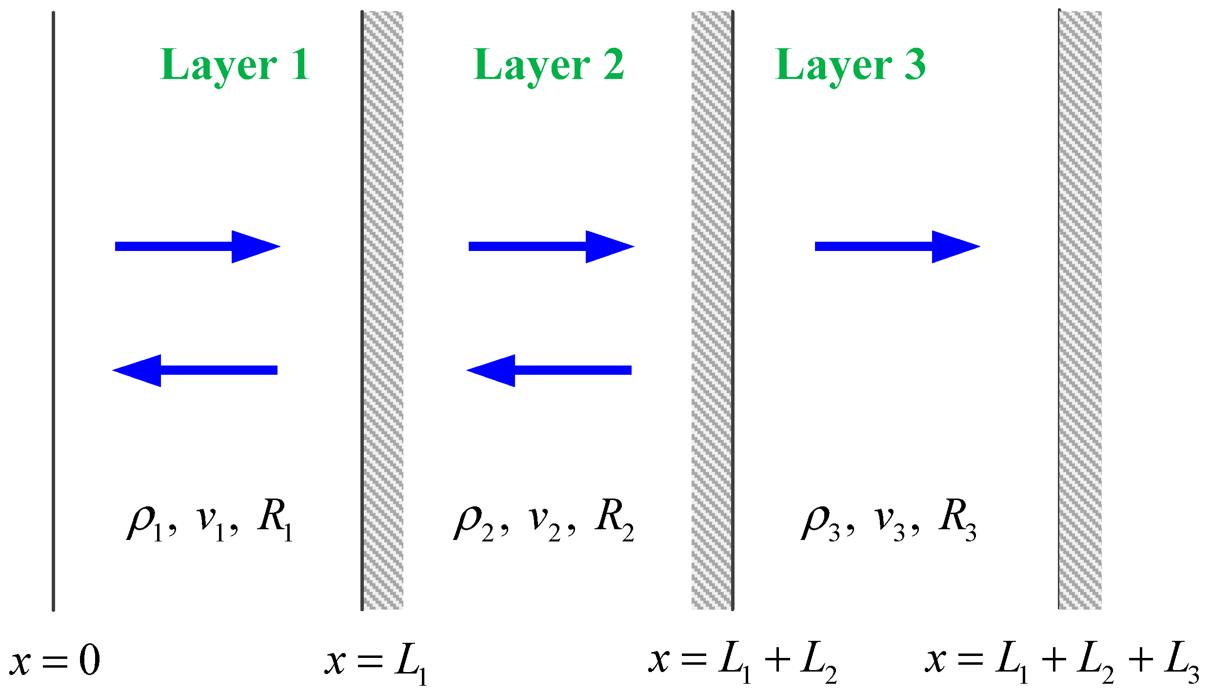
As shown in Figure 1, with the model consists of a composite solid with three parallel layers, labeled by regions 1, 2, and 3, respectively. Each layer has a thickness Lj, for which the subscript j denotes the region number. The one-dimensional coordinate system origin is located at the surface of the composite system. As a result, the interfacial layers are positioned at x = L1 and L1+L2. Each layer material is assumed to be isotropic, homogeneous, and linearly elastic. Although the heterogeneities of the complex tissue–implant–bone system are not taken into consideration, these assumptions for biological tissues can provide acceptable results for ultrasonic thermal therapies [21]. For these three layers, the mass density, the longitudinal wave velocity, and the acoustic characteristic impedance are given, respectively, by ρj, vj, and Rj. The incident acoustic wave was considered to be harmonic with an angular frequency ω so that the velocity potential Φj(x, t) describing the motion in each region is given by
where Re[ ] signifies the real part of the complex number, ϕj(x) is the spatial potential function, and i is the unit imaginary number [22]. Based on linear acoustics, the solutions of the spatial potential function can be solved by the 1-D reduced wave equation, namely
where kj = ω/vj is the wave number.
The acoustic waves, generated by the ultrasound probe, are considered as an infinite train of plane waves horizontally incident from x = 0 [23,24]. For each layer, the pressure fields of the left- or right-going waves can be expressed as follows [25]:
where A1i, A1r, A2i, A2r, and A3i are the unknown amplitude coefficients. The subscripts i and r represent the amplitudes of the incident wave and the reflection wave, respectively. It should be noted that multiple reflections appearing in each medium are neglected for simplicity.
The pressure and velocity continuity conditions must be satisfied on each bilayer interface. This gives rise to a linear system of four equations with four unknowns. Using Cramer’s rule and normalizing yields the following explicit forms:
2.2. Evaluation of Temperature Fields
The focus of this section is solving the transient temperature distribution in a 1-D composite medium with finite thickness; the overall thickness of the present model is L1 + L2 + L3 (see Figure 1). Mathematically, the conduction of heat into a composite medium with internal heat generation within each layer has to obey
where αj = Kj/(ρ cj) is the thermal diffusivity, cj is the specific heat capacity, Tj is the temperature, t is the time measured in seconds, Kj is the thermal conductivity, and qj is the volumetric rate of heat generation.
The molecular vibration in the tissue due to ultrasound will result in temperature change and achieve the therapeutic effect. The volumetric heat generation rate, qj, which results from the propagation of ultrasound can be calculated from the computed pressure by [26]:
where aj stands for the attenuation coefficient, and Pj is the pressure resulted from the ultrasound diathermy (see Equation (3)). The superscript * represents the conjugate of complex numbers.
The composite system is initially set at a uniform temperature, hence, the initial conditions are
Without losing generality, the front surface (at x = 0) of the composite system is exposed to a change in the temperature up until Tend after heating [27]. In addition, the rear surface is set as adiabatic, resulting in the corresponding boundary conditions,
and
Moreover, the temperature matching condition across the interface between adjacent layers is given by
and the heat-flux matching condition that assures perfect thermal contact is
The analytical solution for the one-dimensional transient heat conduction problem with non-homogeneous boundary conditions can be obtained with the aid of the orthogonal expression technique and a Green’s function approach [28]. More details of the derivation are listed in the Appendix A.
3. Results and Discussions
In the following numerical simulations, the initial temperature of the composite specimen was set to be 26 °C and the final temperature on the front surface, Tend, was also set to 26 °C. The computed temperature profile, according to the analytical solution, is assumed along the acoustic axis of the ultrasound probe. In addition, it is worth noting that the volumetric rate of heat generation in Equation (6) was calibrated by the factor A1i with values of 1.9 × 10⁵ and 1.25 × 10⁵ to fit the results of the in vitro experiments under 1 MHz and 3 MHz ultrasound thermal therapy [12], respectively. It is worth noting that the following investigation is based on a simplified theoretical model in which all media are homogeneous and parallel slabs. The effects of the scattering and reflection of ultrasound due to heterogeneities in media and uneven surfaces are neglected in this study.
3.1. Ultrasound Operation Frequency
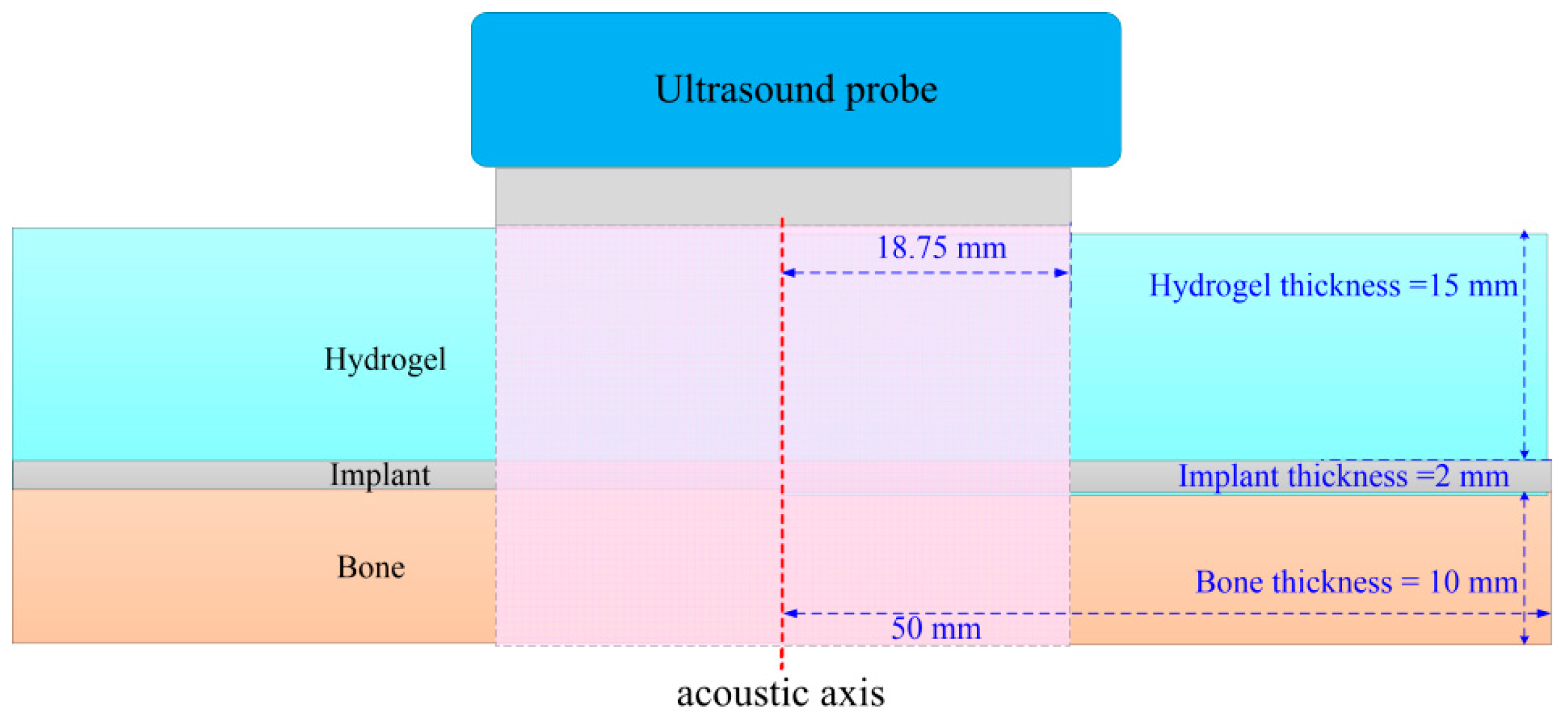
The hydrogel-implant-bone composite specimen in the literature [12] was selected as the benchmark example. The transparent hydrogel layer has a thickness of 15 mm. The metal implant, made of 316 stainless steel, has a thickness of 2 mm. The average thickness of the flat bovine bone is about 10 mm. The material properties of the hydrogel phantom, metal implant, and bone used in the analytical solutions and numerical simulations are listed in Table 1.
In addition to the proposed analytical solution, two-dimensional finite element models were also created to simulate the in vitro experiments using the commercial finite element package Abaqus [29]. A two-dimensional finite-element model was constructed using quadratic thermal elements (D2TH8 in Abaqus) with an element size of 1 × 10⁻⁴ m. The dimensions of the hydrogel–implant–bone system are shown in Figure 2. The front surface of the composite system was set to a constant initial temperature while the other three outer surfaces were set as adiabatic. The area beneath the ultrasound probe was the heating region with the heat source given by Equation (6). The time increment was 0.5 s in the thermal transient analyses.
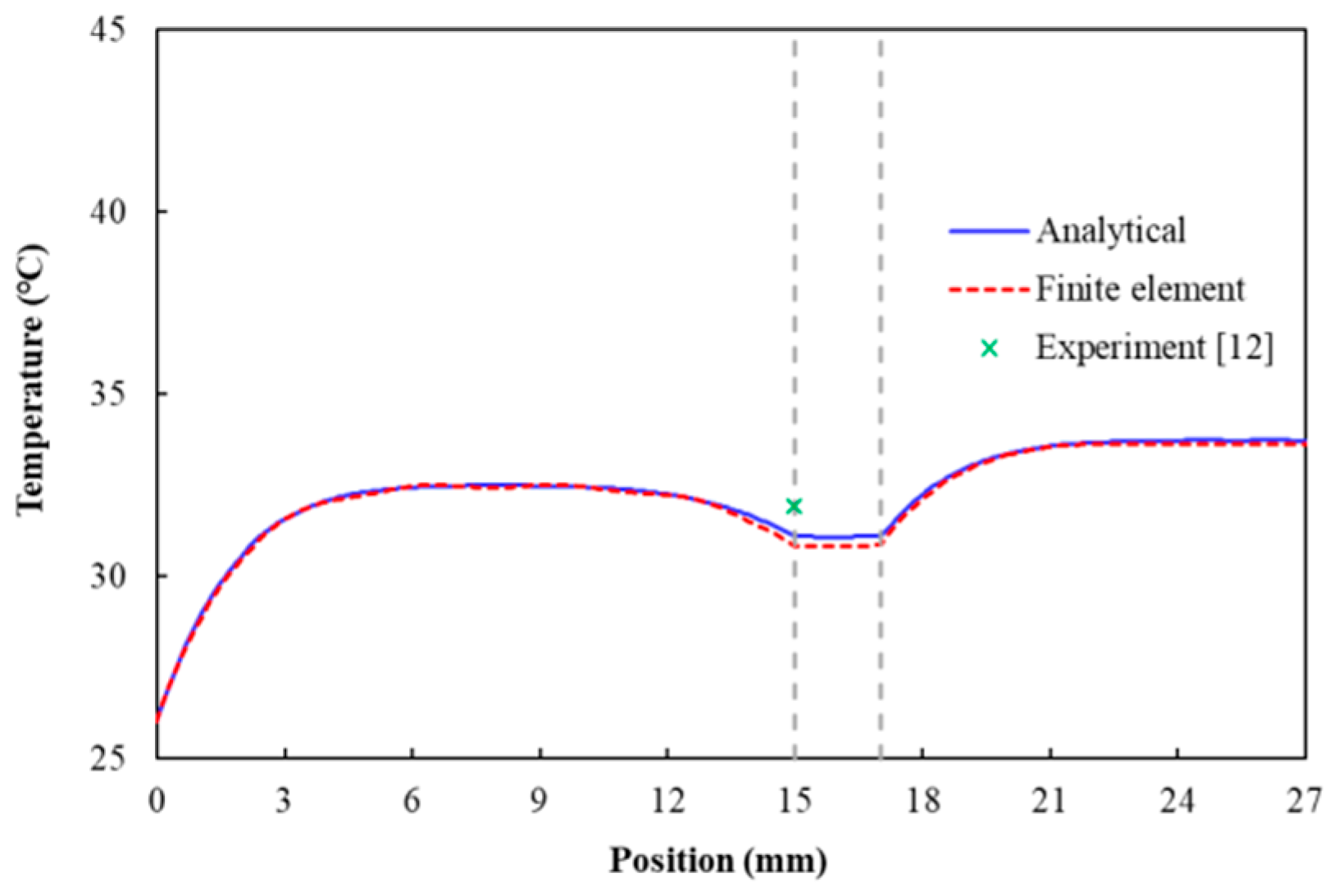
Figure 3 and Figure 4 show the temperature distribution along the acoustic axis at 30 s during the ultrasound diathermy corresponding to 1 MHz and 3 MHz, respectively. For an operational ultrasound frequency of 1 MHz, the peak temperature occurs in the hydrogel phantom of the bio-composite system. Alternatively, the peak temperature occurs in the bone of the bio-composite system for an operational frequency of 3 MHz. In addition, the peak temperature in the hydrogel under 1 MHz is slightly higher than that in the hydrogel under 3 MHz. The peak temperature in the bone under 3 MHz is higher than that in the bone under 1 MHz. As shown in Figure 3 and Figure 4, the analytical results coincide well with the numerical results from Abaqus. These two figures provide sufficient evidence to demonstrate the accuracy of the proposed analytical solutions.
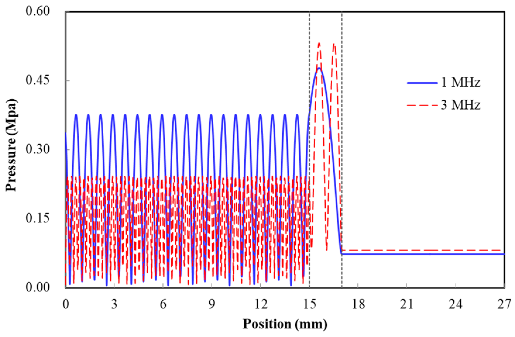
Since material and geometric properties of these two composite systems are the same, the differences in temperature distribution in Figure 3 and Figure 4 mainly resulted from the changes in the pressure field under different ultrasound operation frequencies. Figure 5 shows the pressure amplitude distributions along the acoustic axis corresponding to 1 MHz and 3 MHz. One can observe that the pressure amplitude in hydrogel for 1 MHz is higher than that for 3 MHz, which implies that more energy is input into the hydrogel in the case of 1 MHz and the ultrasound of 1 MHz can propagate deeper in tissues. As a result, the temperature in hydrogel in the case of 1 MHz is higher than that for 3 MHz. However, the temperature in the stainless implant for 1 MHz is higher than that for 3 MHz, although the pressure amplitude in the implant for 1 MHz is lower than that for 3 MHz. This result is likely because the temperature in the medium depends not only on the input energy from the heat source but also on the heat conduction from the neighboring medium (hydrogel). Finally, since the area enclosed by the pressure amplitude curve in the bone layer for 1 MHz is smaller than that for 3 MHz, the temperature in bone layer for 1 MHz is lower than that for 3 MHz.
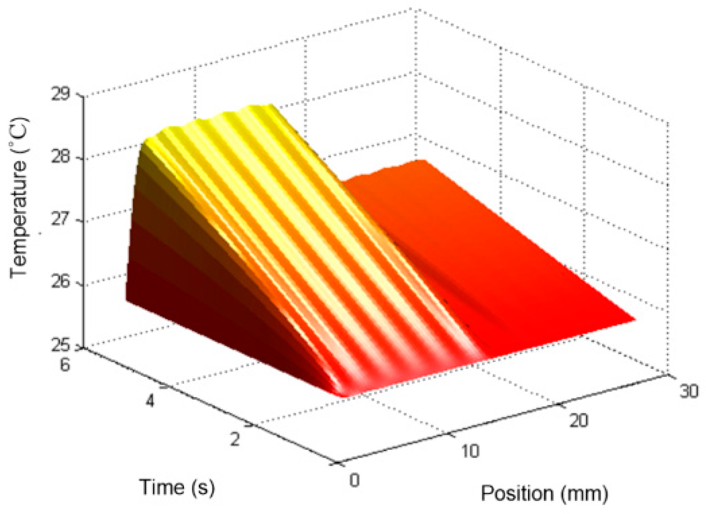
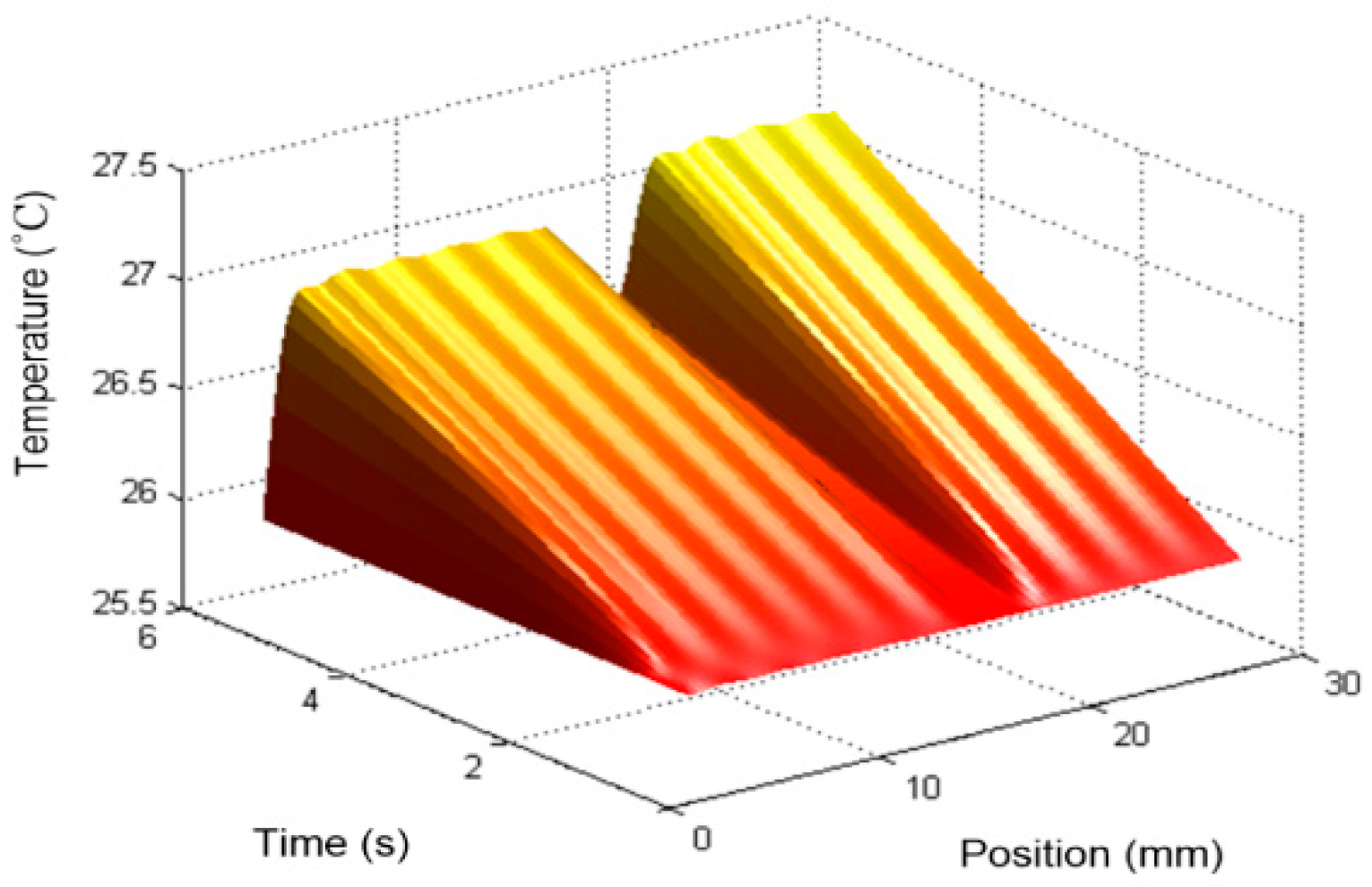
Figure 6 and Figure 7 represent the temperature distribution, obtained from the analytical solution, in the three-layer composite system in the first five seconds corresponding to the low (1 MHz) and high (3 MHz) ultrasound frequencies, respectively. As observed in Figure 6 and Figure 7, the standing wave pattern occurred in the hydrogel layer. These results explain the light and dark parallel patterns of standing waves in front of a reflective stainless steel plate in water bath experiments [2]. In addition, the amplitudes of the temperature oscillations decreased with increasing ultrasound frequency. The temperature variation amplitudes gradually reduced along both the spatial and temporal directions. The amplitude reduction in the temporal direction occurred faster as compared to the spatial direction. Moreover, the amplitudes of the temperature oscillations were smaller than the temperature variation in the hydrogel during ultrasound diathermy. As a result, the small temperature oscillations cannot be easily observed in the in vitro or ex vivo experiments.
3.2. Tissue Thickness
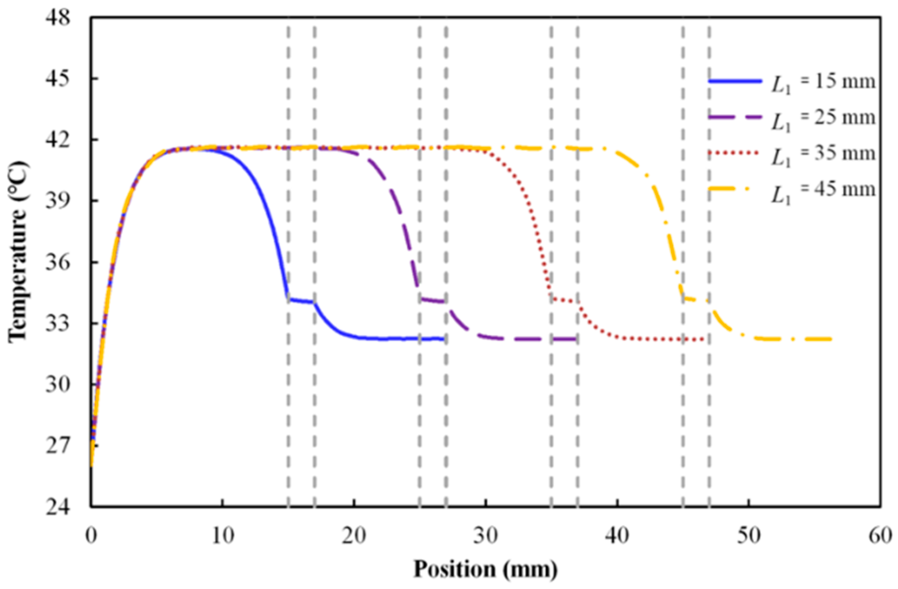
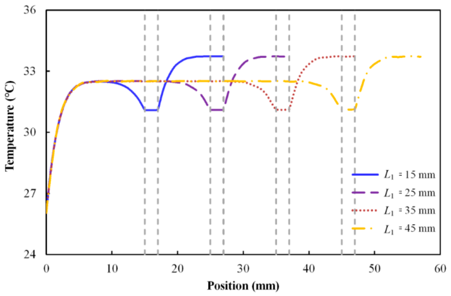
The thicknesses of tissues, which may affect the ultrasound thermal therapy, are different from person to person. As a result, the effects of the hydrogel phantom thickness on the temperature variation were investigated. The three-layer composite systems were simulated for ultrasound diathermy with 30 s at a power of 15 W and 12 W using 1 MHz and 3 MHz, respectively. Figure 8 and Figure 9 show the simulated results of the temperature profiles in the composite specimens with a stainless steel implant and different thicknesses hydrogel phantom under 1 MHz and 3 MHz ultrasound operation frequencies.
For the cases of 1 MHz, the peak temperature location predicted by the analytical solution occurs at the middle region of the hydrogel phantom in the composite system. It is worth noting that the peak temperature does not change depending on different hydrogel thickness. However, the region with the peak temperature in the hydrogel has greater expansion with increasing thickness of the hydrogel in the composite system. Approaching the interface between the hydrogel and the stainless implant, the temperature decreases and continues to decrease in the bone of the composite system as shown in Figure 8.
Alternatively, the peak temperature location predicted by the analytical solution is always in the bone for the case of 3 MHz as shown in Figure 9. Similarly, the peak temperature in each layer does not change with different hydrogel thicknesses. However, the region of the peak local temperature in the hydrogel expands more with increasing thickness of the hydrogel. Close to the interface between the hydrogel and the stainless implant, the temperature decreases, but the temperature keeps increasing in the bone of the composite system.
These results can be explained by the pressure distribution curves, as shown in Figure 5, where the pressure oscillation does not change in the composite system media. In addition, the amplitude of the heat source in each medium, according to Equations (A1) and (A2), is related to the thickness of the implant, and not to the thickness of the hydrogel. As a result, the highest temperature in the media remains the same with different hydrogel thicknesses.
3.3. Implant Materials
Since the influences of implants on the temperature distribution during ultrasound diathermy can be studied from analytical solutions, another important issue for implants in clinical applications is the selection of implant materials. In recent years, the list of potential materials for surgical implants has been notably expanded. However, the effects of these new implant materials on ultrasound diathermy are still unknown. To enhance the safety in clinical applications, it is important to get more understanding of the responses of ultrasound thermal therapies using new implant materials.
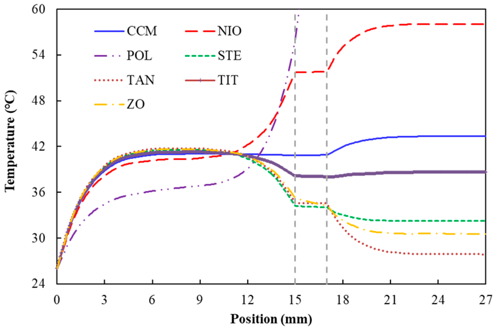
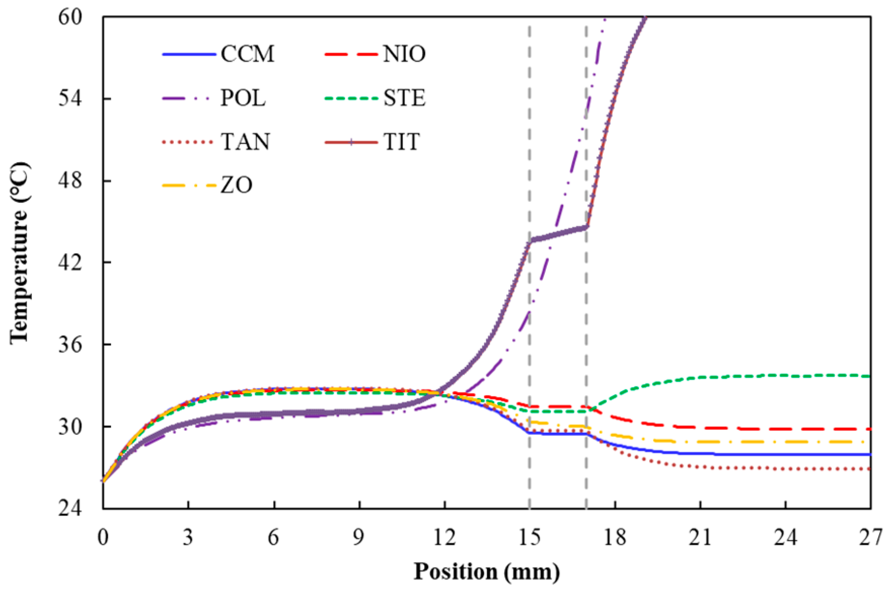
Five metals (Stainless steel, Tantalum, Titanium alloys, Co-Cr-Mn Alloy, Niobium), one plastic (Polyethylene), and one ceramic implant (Zirconia Oxide), for which material properties are listed in Table 2 and Table 3, were selected. These seven implant materials are denoted as ‘STE’, ‘TAN’, ‘TIT’, ‘CCM’, ‘NIO’, ‘POL’, and ‘ZO’ for short. Typical simulation results for the temperature distribution within the composite specimen, obtained from the analytical solution, are presented in Figure 10 and Figure 11, which correspond to 1 MHz and 3 MHz ultrasound operation frequency, respectively. The duration of the heating process was 30 s. The location of the implant is indicated by dashed gray lines in Figure 10 and Figure 11.
As observed in Figure 10 and Figure 11, the obtained results show a rising trend when the value of x ranged between 0 and 8 mm. As opposed to the polymer implant, the temperature responses of the metal and ceramic implants were very close when x < 10 mm. In the case of Polyethylene (POL), the temperature rose considerably in the implant and bone region. The peak temperature of the POL case was above 65 °C and 125 °C for 1 MHz and 3 MHz, respectively, at 30 s. Therefore, ultrasound should avoid near polymer implants. Alternatively, the average temperature of the Tantalum (TAN) was under 25 °C in the bone region, while in the tissue region it was also the minimum. As a result, the use of Tantalum in implants is preferred with regard to ultrasound diathermy. It is worth emphasizing that only thermal responses were considered in this study. One may consider mechanical properties, surface properties, and biocompatibility in clinical performances to determine the optimal implant material.
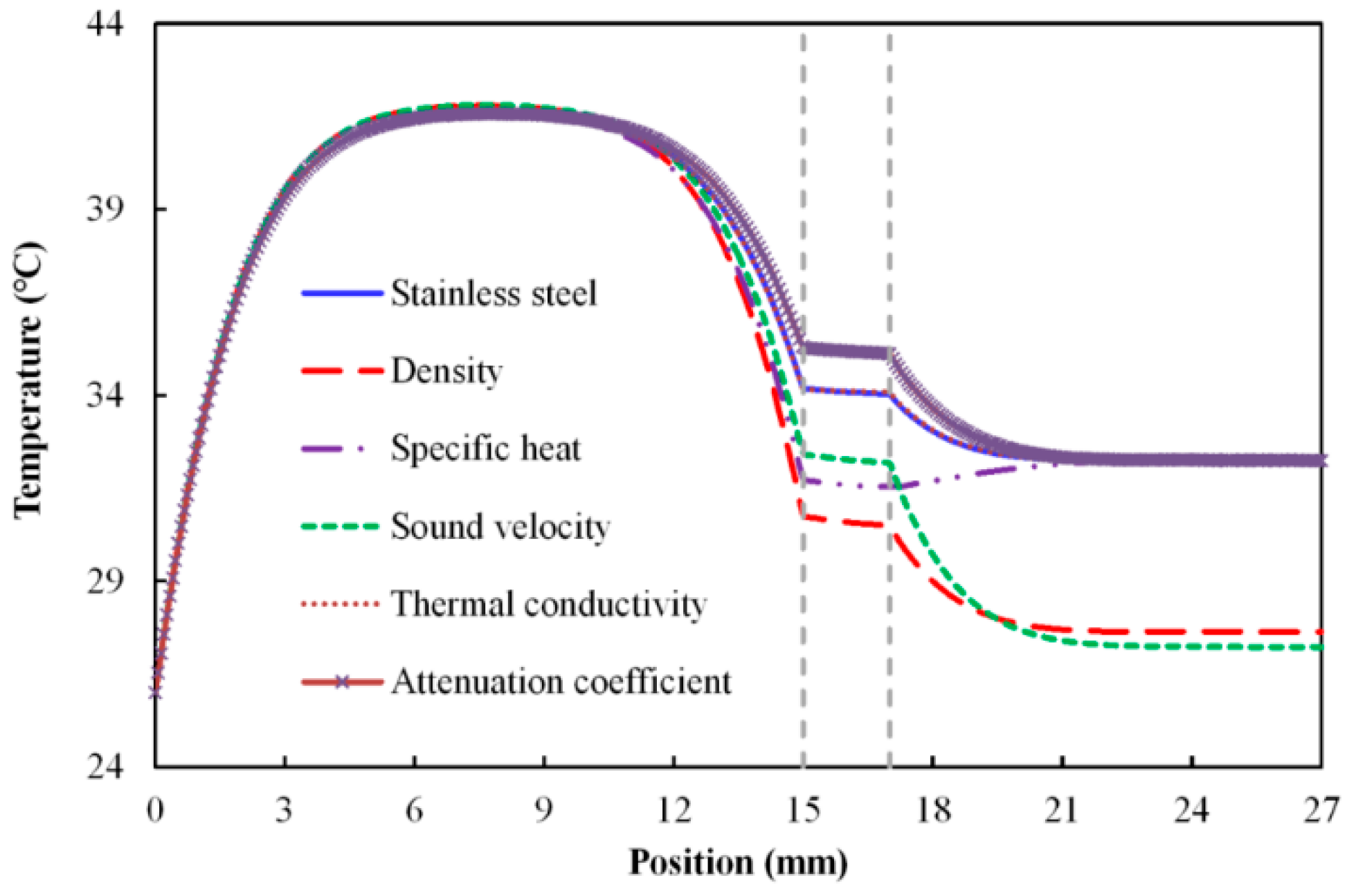
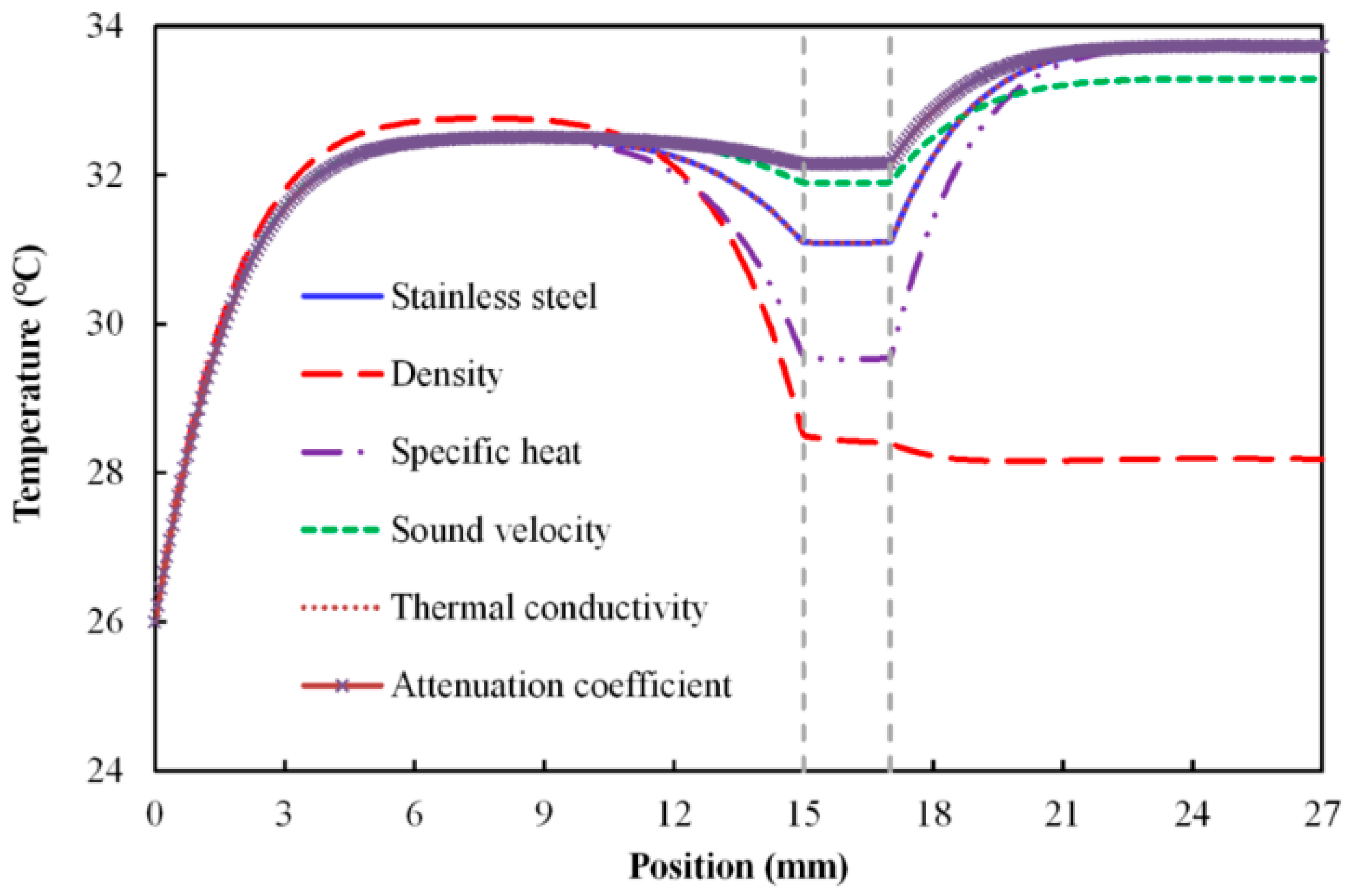
Furthermore, to determine which material property has the most influence on the temperature distribution, sensitivity analyses were performed to investigate the effects of five material properties of the stainless steel—density, specific heat, sound velocity, thermal conductivity, and attenuation coefficient—on the temperature distribution during the ultrasound diathermy. Figure 12 and Figure 13 show the temperature distribution along the acoustic axis at 30 s during the ultrasound diathermy, corresponding to 1 MHz and 3 MHz, respectively. Each temperature curve represents an increase of a specific material property to two times that of the stainless steel while keeping other material properties the same as those of the stainless steel. Figure 12 and Figure 13 show that an increase in the attenuation coefficient increases the temperature in the composite system during the ultrasound diathermy. However, the increases in the density and specific heat cause the temperature in the composite system to decrease during the ultrasound diathermy. Finally, the increase of the thermal conductivity seems not to affect the temperature in the composite system during the ultrasound diathermy. The increase of the sound velocity may increase or decrease the temperature in the composite system depending on the ultrasound operation frequency.
4. Conclusions
In this study, a tissue-implant-bone specimen was modeled as a composite system with three parallel layers. This simplified system can be used to investigate the influences of an implant on the temperature field in tissues during ultrasound thermal therapy and provides a better selection of implant materials from thermodynamics. An analytical solution was derived for the one-dimensional transient heat conduction problem using the orthogonal expansion technique and a Green’s function approach. The accuracy of the derived analytical solution was verified by in vitro experimental results [12] and finite element numerical simulations.
The analytical solution explained well the pattern of standing waves in the beginning of the ultrasound diathermy and the disappearance of these standing waves during longer duration (above 1 min) thermal application. In addition, while the thickness of the hydrogel layer does not change the highest temperature in each layer during ultrasound diathermy, it only changes the temperature distribution profile. Furthermore, a parametric study conducted through analytical solutions indicates that materials with high density, high specific heat, and low thermal conductivity may be suitable implant materials. Since most materials lack all these features, the tantalum implant is a good choice among the available implant materials as a lower temperature rise can be achieved within the hydrogel and bone layers during ultrasound diathermy.
Funding
This research was funded by the Ministry of Science and Technology (106-2221-E-033-034-MY3 and 108-2218-E-080-001), Republic of China (Taiwan).
Acknowledgments
The author acknowledges the financial support of the Ministry of Science and Technology (106-2221-E-033-034-MY3 and 108-2218-E-080-001), Republic of China (Taiwan). The author is also grateful to Simutech Solution Corporation (Taiwan) for providing the computational resources.
Conflicts of Interest
The author declares no conflict of interest. The funders had no role in the design of the study; in the collection, analyses, or interpretation of data; in the writing of the manuscript, or in the decision to publish the results.
Appendix A
Substituting Equation (3) into Equation (6), one can obtain an explicit form for heat generation from ultrasound:
with
Equation (5) and Equations (7)–(10) present a 1-D transient heat conduction problem with nonhomogeneous boundary conditions. The nonhomogeneous boundary condition in Equation (8a) can be overcome by shifting the temperature scale. By setting , a new formulation with homogeneous boundary conditions can be found as follows.
with initial conditions:
The solution of Equation (A3) can be obtained by solving the homogeneous transient heat conduction problem by first neglecting the heat generation in Equation (A3a). From the separation of variables method, the shifted temperature fields without heat generation can be separated as
Substituting Equation (A4) into Equation (A3a), one can obtain
The separation given by Equation (A5) results in two ordinary differential equations for the determination of the time-dependent function Γ(t) and the space-dependent function ψj(x) in each layer. For parallel layers, the general solution of the space-dependent function ψj(x) in each layer can be obtained by solving the corresponding eigenvalue problem,
where An, Bn, Cn, and Dn are unknown coefficients which can be determined from the boundary conditions in Equations (A3b)–(A3e). For An = 1,
with
In addition, βn are the eigenvalues satisfying the following transcendental equation:
with
The solution of the time-dependent function Γ(t) in Equation (A5) is
where Γn is an undetermined coefficient. Substituting Equation (A9) back into Equation (A4) and substituting the initial conditions, one can obtain the temperature distribution without internal heat generation in each layer, that is
where Γn is given by
with
Finally, the effects of heat generation within each layer can be considered by utilizing a Green’s function approach [25]. Referring to Equation (A10), one may get the start-up Green’s function of each layer. When multiplying Equations (A6a)–(A6c) respectively, by Equations (A1a)–(A1c) and then integrating with respect to x, one can obtain the temperature distribution Θh,j(x, t) induced by ultrasound heat generation within each layer, that is
where
with
and
Summing up the above derivations, the temperature field in each layer of the one-dimensional composite system is given by
References
- Cameron, M.H. Physical Agents in Rehabilitation: From Research to Practice, 4th ed.; Elsevier Health Sciences: USA, 2012; pp. 185–214. [Google Scholar]
- Lehmann, J.F.; Lane, K.E.; Bell, J.W.; Brunner, G.D. Influence of surgical metal implants on the distribution of the intensity in the ultrasonic field. Arch. Phys. Med. Rehabil. 1958, 39, 756–760. [Google Scholar] [CrossRef]
- Rose, S.; Draper, D.O.; Schulthies, S.S.; Durrant, E. The stretching window part two: Rate of thermal decay in deep muscle following 1-MHz ultrasound. J. Athl. Train. 1996, 31, 139–143. [Google Scholar] [CrossRef]
- Denegar, C.R.; Saliba, E.; Saliba, S. Therapeutic Modalities for Musculoskeletal Injuries, 4th ed.; Human Kinetics: Champaign, IL, USA, 2015; pp. 1–42. [Google Scholar]
- Morishita, K.; Karasuno, H.; Yokoi, Y.; Morozumi, K.; Ogihara, H.; Ito, T.; Hanaoka, M.; Fujiwara, T.; Fujimoto, T.; Abe, K. Effects of therapeutic ultrasound on range of motion and stretch pain. J. Phys. Ther. Sci. 2014, 26, 711–715. [Google Scholar] [CrossRef] [PubMed] [Green Version]
- Analan, P.D.; Leblebici, B.; Adam, M. Effects of therapeutic ultrasound and exercise on pain, function, and isokinetic shoulder rotator strength of patients with rotator cuff disease. J. Phys. Ther. Sci. 2015, 27, 3113–3117. [Google Scholar] [CrossRef] [PubMed]
- Zhang, C.; Xie, Y.; Luo, X.; Ji, Q.; Lu, C.; He, C.; Wang, P. Effects of therapeutic ultrasound on pain, physical functions and safety outcomes in patients with knee osteoarthritis: A systematic review and meta-analysis. Clin. Rehabil 2016, 30, 960–971. [Google Scholar] [CrossRef] [PubMed]
- Baker, K.G.; Robertson, V.J.; Duck, F.A. A review of therapeutic ultrasound: Biophysical effects. J. Womens Health Phys. Ther. 2010, 34, 111–118. [Google Scholar] [CrossRef]
- Gersten, J.W. Effect of metallic objects on temperature rises produced in tissue by ultrasound. Am. J. Phys. Med. Rehabil. 1958, 37, 75–82. [Google Scholar] [CrossRef]
- Lehmann, J.F.; Brunner, G.D.; McMillan, J.A. Influence of surgical metal implants on the temperature distribution in thigh specimens exposed to ultrasound. Arch. Phys. Med. Rehabil. 1958, 39, 692–695. [Google Scholar] [CrossRef]
- Lehmann, J.F.; Brunne, G.D.; Martinis, A.J.; McMillan, J.A. Ultrasonic effects as demonstrated in live pigs with surgical metallic implants. Arch. Phys. Med. Rehabil. 1659, 40, 483–488. [Google Scholar] [CrossRef]
- Sun, M.K.; Shieh, J.; Chen, C.S.; Chiang, H.G.; Huang, C.W.; Chen, W.S. Effects of an implant on temperature distribution in tissue during ultrasound diathermy. Ultrason. Sonochem. 2016, 32, 44–53. [Google Scholar] [CrossRef]
- Andrades, A.O.; Mazzanti, A.; Beckmann, D.V.; Aiello, G.; Chaves, R.O.; Santos, R.P. Heating produced by therapeutic ultrasound in the presence of a metal plate in the femur of canine cadavers. Arq. Bras. Med. Vet. Zootec. 2014, 66, 1343–1350. [Google Scholar] [CrossRef]
- Hsu, S.K.; Huang, W.T.; Liu, B.S.; Li, S.M.; Chen, H.T.; Chang, C.J. Effects of near-field ultrasound stimulation on new bone formation and osseointegration of dental titanium implants in vitro and in vivo. Ultrasound Med. Biol. 2011, 37, 403–416. [Google Scholar] [CrossRef] [PubMed]
- Schröder, C.; Steinbrück, A.; Müller, T.; Woiczinski, M.; Chevalier, Y.; Weber, P.; Müller, P.E.; Jansson, V. Rapid prototyping for in vitro knee rig investigations of prosthetized knee biomechanics: Comparison with cobalt-chromium alloy implant material. BioMed Res. Int. 2015, 2015, 185142. [Google Scholar] [CrossRef] [Green Version]
- Öztürk, S.; Sengezer, M.; Zor, F. Reconstruction of acquired partial auricular defects by porous polyethylene implant and superficial temporoparietal fascia flap in adult patients. Plast. Reconstr. Surg. 2006, 118, 1349–1357. [Google Scholar] [CrossRef]
- Vainionpää, S.; Rokkanen, P.; Törmälä, P. Surgical applications of biodegradable polymers in human tissues. Prog. Polym. Sci. 1989, 14, 679–716. [Google Scholar] [CrossRef]
- Kienapfel, H.; Sprey, C.; Wilke, A.; Griss, P. Implant fixation by bone ingrowth. J. Arthroplast. 1999, 14, 355–368. [Google Scholar] [CrossRef]
- Iwai, T.; Harada, Y.; Imura, K.; Iwabuchi, S.; Murai, J.; Hiramatsu, K.; Myoui, A.; Yoshikawa, H.; Tsumaki, N. Low-intensity pulsed ultrasound increases bone ingrowth into porous hydroxyapatite ceramic. J. Bone Miner. Metab. 2007, 25, 392–399. [Google Scholar] [CrossRef]
- Adams, T.S.; Crook, T.; Cadier, M.A. A late complication following the insertion of hydrogel breast implants. J. Plast. Reconstr. Aesthet. Surg. 2007, 60, 210–212. [Google Scholar] [CrossRef]
- Lints, M. Optimised Signal Processing for Nonlinear Ultrasonic Nondestructive Testing of Complex Materials and Biological Tissues. Ph.D. Thesis, Tallinn University of Technology, Tallinn, Estonia, 2017. [Google Scholar]
- Kinsler, L.E.; Frey, A.R.; Coppens, A.B.; Sanders, J.V. Fundamentals of Acoustics, 4th ed.; John Wiley & Sons: New York, NY, USA, 1999; pp. 171–203. [Google Scholar]
- Zhou, Y. Principles and Applications of Therapeutic Ultrasound in Healthcare; CRC Press: Boca Raton, FL, USA; Taylor & Francis Group: Oxfordshire, UK, 2016; p. 129. [Google Scholar]
- Shaw, A.; Hodnett, M. Calibration and measurement issues for therapeutic ultrasound. Ultrasonics 2008, 48, 234–252. [Google Scholar] [CrossRef]
- Blackstock, D.T. Fundamentals of Physical Acoustics; John Wiley & Sons: New York, NY, USA, 2000; pp. 163–172. [Google Scholar]
- Meaney, P.M.; Clarke, R.L.; Ter Haar, G.R.; Rivens, I.H. A 3-D finite-element model for computation of temperature profiles and regions of thermal damage during focused ultrasound surgery exposures. Ultrasound Med. Biol. 1998, 24, 1489–1499. [Google Scholar] [CrossRef]
- Schimmel, W.P.; Beck, J.V.; Donaldson, A.B. Effective thermal diffusivity for a multimaterial composite laminate. J. Heat Transfer 1977, 99, 466–470. [Google Scholar] [CrossRef]
- Hahn, D.W.; Özisik, M.N. Heat Conduction, 3rd ed.; John Wiley & Sons: New York, NY, USA, 2012; pp. 393–430. [Google Scholar]
- SIMULIA-Abaqus 2017 User’s Manual; Dassault Systemes Simulia: Providence, RI, USA, 2017.
- Xi, F.; Jin, K.; Cai, L.; Geng, H.; Tan, Y.; Li, J. Sound velocity of tantalum under shock compression in the 18–142 GPa range. J. Appl. Phys. 2015, 117, 185901. [Google Scholar] [CrossRef]
- Veiga, C.; Davim, J.P.; Loureiro, A.J.R. Properties and applications of titanium alloys: A brief review. Rev. Adv. Mater. Sci. 2012, 32, 133–148. [Google Scholar] [CrossRef]
- Baron, S.; Desmond, D.; Ahearne, E. The fundamental mechanisms of wear of cemented carbide in continuous cutting of medical grade cobalt chromium alloy (ASTM F75). Wear 2019, 424, 89–96. [Google Scholar] [CrossRef]
- Grill, R.; Gnadenberger, A. Niobium as mint metal: Production–properties–processing. Int. J. Refract. Metals Hard Mater. 2006, 24, 275–282. [Google Scholar] [CrossRef]
- Guo, S.Q. Densification of ZrB2-based composites and their mechanical and physical properties: A review. J. Eur. Ceram. Soc. 2009, 29, 995–1011. [Google Scholar] [CrossRef]
- Zhang, Y.; Malzbender, J.; Mack, D.E.; Jarligo, M.O.; Cao, X.; Li, Q.; Vaßen, R.; Stöver, D. Mechanical properties of zirconia composite ceramics. Ceram. Int. 2013, 39, 7595–7603. [Google Scholar] [CrossRef]
Figure 1.
Schematic layout of a three-layer composite medium subjected to ultrasound waves.

Figure 2.
Dimensions of the composite sample model consisted of bone, implant, and hydrogel layer.

Figure 3.
Temperature distribution along the acoustic axis from the proposed analytical solution and numerical simulation at 30 s using 1 MHz ultrasound.
Figure 3.
Temperature distribution along the acoustic axis from the proposed analytical solution and numerical simulation at 30 s using 1 MHz ultrasound.

Figure 4.
Temperature distribution along the acoustic axis from the proposed analytical solution and numerical simulation at 30 s using 3 MHz ultrasound.
Figure 4.
Temperature distribution along the acoustic axis from the proposed analytical solution and numerical simulation at 30 s using 3 MHz ultrasound.

Figure 5.
Pressure distribution along the acoustic axis from the proposed analytical solution for 1 MHz and 3 MHz ultrasounds.
Figure 5.
Pressure distribution along the acoustic axis from the proposed analytical solution for 1 MHz and 3 MHz ultrasounds.

Figure 6.
Temperature profiles in the composite bio-system from the proposed analytical solution in the first five seconds using 1 MHz ultrasound.
Figure 6.
Temperature profiles in the composite bio-system from the proposed analytical solution in the first five seconds using 1 MHz ultrasound.

Figure 7.
Temperature profiles in the composite bio-system from the proposed analytical solution in the first five seconds using 3 MHz ultrasound.
Figure 7.
Temperature profiles in the composite bio-system from the proposed analytical solution in the first five seconds using 3 MHz ultrasound.

Figure 8.
Temperature distribution within the three-layer composite bio-system for different hydrogel thickness at 30 s using 1 MHz ultrasound.
Figure 8.
Temperature distribution within the three-layer composite bio-system for different hydrogel thickness at 30 s using 1 MHz ultrasound.

Figure 9.
Temperature distribution within the three-layer composite bio-system for different hydrogel thickness at 30 s using 3 MHz ultrasound.
Figure 9.
Temperature distribution within the three-layer composite bio-system for different hydrogel thickness at 30 s using 3 MHz ultrasound.

Figure 10.
Temperature distribution within the three-layer composite bio-system for various implants at 30 s using 1 MHz ultrasound.
Figure 10.
Temperature distribution within the three-layer composite bio-system for various implants at 30 s using 1 MHz ultrasound.

Figure 11.
Temperature distribution within the three-layer composite bio-system for various implants at 30 s using 3 MHz ultrasound.
Figure 11.
Temperature distribution within the three-layer composite bio-system for various implants at 30 s using 3 MHz ultrasound.

Figure 12.
Temperature distribution within the three-layer composite bio-system for different material properties at 30 s using 1 MHz ultrasound.
Figure 12.
Temperature distribution within the three-layer composite bio-system for different material properties at 30 s using 1 MHz ultrasound.

Figure 13.
Temperature distribution within the three-layer composite bio-system for different material properties at 30 s using 3 MHz ultrasound.
Figure 13.
Temperature distribution within the three-layer composite bio-system for different material properties at 30 s using 3 MHz ultrasound.


Table 1.
Material properties of the N-isopropyl acrylamide (NIPAM)-based hydrogel phantom, implants, and bone [12].
Table 1.
Material properties of the N-isopropyl acrylamide (NIPAM)-based hydrogel phantom, implants, and bone [12].
| Hydrogel Phantom | 316 Stainless Steel | Bone | |
|---|---|---|---|
| Density (kg/m3) | 1190 | 8000 | 1975 |
| Specific heat (J/kg°C) | 3431 | 502 | 1313 |
| Sound velocity (m/s) | 1512 | 5600 | 3476 |
| Thermal conductivity (W/m°C) | 0.6 | 16.27 | 0.32 |
| Attenuation coefficient (dB/m) | 54 | 110 | 690 |
Table 2.
Material properties of the different implant materials (polymer and metal).
| Polyethylene (POL) [12] | Tantalum (TAN) [30] | Titanium Alloys (TIT) [31] | |
|---|---|---|---|
| Density (kg/m3) | 960 | 16,650 | 4470 |
| Specific heat (J/kg°C) | 2300 | 141.8 | 561 |
| Sound velocity (m/s) | 2460 | 5374 | 6132 |
| Thermal conductivity (W/m°C) | 0.442 | 57 | 7.2 |
| Attenuation coefficient (dB/m) | 66 | 144 | 150 |
Table 3.
Material properties of the different implant materials (metal and ceramic).
| Co-Cr-Mo Alloy (CCM) [32] | Niobium (NIO) [33] | Zirconia Oxide (ZO) [34,35] | |
|---|---|---|---|
| Density (kg/m3) | 8768 | 8570 | 6050 |
| Specific heat (J/kg°C) | 452 | 265 | 418 |
| Sound velocity (m/s) | 4750 | 3480 | 7040 |
| Thermal conductivity (W/m°C) | 14.8 | 53.70 | 2.7 |
| Attenuation coefficient (dB/m) | 230 | 347 | 120 |
© 2020 by the author. Licensee MDPI, Basel, Switzerland. This article is an open access article distributed under the terms and conditions of the Creative Commons Attribution (CC BY) license (http://creativecommons.org/licenses/by/4.0/).
Share and Cite
MDPI and ACS Style
Huang, C.-W. Simplified Theoretical Model for Temperature Evaluation in Tissue–Implant–Bone Systems during Ultrasound Diathermy. Appl. Sci. 2020, 10, 1306. https://doi.org/10.3390/app10041306
AMA Style
Huang C-W. Simplified Theoretical Model for Temperature Evaluation in Tissue–Implant–Bone Systems during Ultrasound Diathermy. Applied Sciences. 2020; 10(4):1306. https://doi.org/10.3390/app10041306
Chicago/Turabian StyleHuang, Chang-Wei. 2020. "Simplified Theoretical Model for Temperature Evaluation in Tissue–Implant–Bone Systems during Ultrasound Diathermy" Applied Sciences 10, no. 4: 1306. https://doi.org/10.3390/app10041306
Note that from the first issue of 2016, this journal uses article numbers instead of page numbers. See further details here.