Automatic Method for Bone Segmentation in Cone Beam Computed Tomography Data Set
by
 ,
,
Mantas Vaitiekūnas
1,*,†, 
Darius Jegelevičius
1,2,†,
Andrius Sakalauskas
3,† and
Simonas Grybauskas
4,† 1
Biomedical Engineering Institute, Kaunas University of Technology, 51423 Kaunas, Lithuania
2
Department of Electronics Engineering, Kaunas University of Technology, 51367 Kaunas, Lithuania
3
JSC Telemed, 03154 Vilnius, Lithuania
4
Simonas Grybauskas’ Orthognathic Surgery, 03229 Vilnius, Lithuania
*
Author to whom correspondence should be addressed.
†
These authors contributed equally to this work.
Appl. Sci. 2020, 10(1), 236; https://doi.org/10.3390/app10010236
Submission received: 28 November 2019
/
Revised: 16 December 2019
/
Accepted: 20 December 2019
/
Published: 27 December 2019
(This article belongs to the Special Issue Biomaterials for Bone Tissue Engineering)
Abstract
:Due to technical aspects of Cone Beam Computed Tomography (CBCT), the automatic methods for bone segmentation are not widely used in the clinical practice of endodontics, orthodontics, oral and maxillofacial surgery. The aim of this study was to evaluate method’s accuracy for bone segmentation in CBCT data sets. The sliding three dimensional (3D) window, histogram filter and Otsu’s method were used to implement the automatic segmentation. The results of automatic segmentation were compared with the results of segmentation performed by an experienced oral and maxillofacial surgeon. Twenty patients and their forty CBCT data sets were used in this study (20 preoperative and 20 postoperative). Intraclass Correlation Coefficients (ICC) were calculated to prove the reliability of surgeon segmentations. ICC was 0.958 with 95% confidence interval [0.896 ... 0.983] in preoperative data sets and 0.931 with 95% confidence interval [0.836 ... 0.972] in postoperative data sets. Three basic metrics were used in order to evaluate the accuracy of the automatic method—Dice Similarity Coefficient (DSC), Root Mean Square (RMS), Average Distance Error (ADE) of surfaces mismatch and additional metric in order to evaluate computation time of segmentation was used. The mean value of preoperative DSC was 0.921, postoperative—0.911, the mean value of preoperative RMS was 0.559 mm, postoperative—0.647 mm, the ADE value of preoperative cases was 0.043 mm, postoperative—0.057 mm, the mean computational time to perform the segmentation was 46 s. The automatic method showed clinically acceptable accuracy results and thus can be used as a new tool for automatic bone segmentation in CBCT data. It can be applied in oral and maxillofacial surgery for performance of 3D Virtual Surgical Plan (VSP) or for postoperative follow-up.
1. Introduction
Three dimensional (3D) segmentation of bones from Cone Beam Computed Tomography (CBCT) is very important for the orthodontics, endodontics, oral and maxillofacial surgeons. Accuracy of segmentation ensures a correct diagnosis, an accurate 3D Virtual Surgical Plan (VSP) and a successful postoperative follow-up of the patients with Cranio-maxillofacial (CMF) deformities [1,2]. Application of CBCT imaging modality in oral and maxillofacial surgery is increased due to its lower radiation dose and shorter acquisition time compared with the conventional multislice CT (MSCT). However, images of CBCT most often are noisier and have beam hardening artifacts. Properties of CBCT also affect the ability to correctly display Hounsfield units (HU) of head tissues (immediately after surgery when edema of soft tissues is present) as opposed to traditional CT [3,4]. These disadvantages also influence image quality and accuracy of bone segmentation [5]. Due to these reasons, 3D VSP and evaluation of postoperative follow-up must be performed using segmentation by highly experienced experts. Such a procedure of bone segmentation becomes time-consuming [6].
Wang et al. published three studies dedicated to fully automatic bone segmentation using CBCT images [6,7,8]. In 2013 [6] and 2014 [7] studies, the principle of the automatic method was a patch-based sparse representation. Patient-specific atlas (probability map) using a sparse label fusion strategy from conventional CT atlases was used as a first estimation. Then a convex segmentation framework was used in order to get the final result. The introduced method led to an accurate segmentation but the basic limitation of this method was computation time (about 5 h [7]). Also, the variety of CBCT data sets (patients with metallic implants, metallic plates and different face deformities) was low in their studies. Data collection of CT to get more variety of the atlases is complicated in relation to the requirements of bioethics. In a 2016 study [8], the same authors also suggested a new automatic method that used the random forest. The multiclass classifier was used to create probability maps for each region of interest (mandible, maxilla and background). The results of the method were achieved almost the same as in the previous study [7] but also with some similar limitations: the limited amount of CBCT data and also computation time of segmentation (20 min). Gollmer and Buzug presented a fully automatic method for mandible segmentation. Segmentation was based on the idea of using a statistical shape model (SSM). They showed accurate results, however, they also—as did the previous authors—tested the algorithm with just six CBCT data sets [9]. Fan et al. [10] proposed an automatic method for mandible segmentation. Marker-based watershed transform method was used in their study. The authors performed accurate and fast enough (12-14 min per data set) segmentation on 20 CBCT data sets. The errors of segmentation were obtained mostly in these three basic areas—around the wisdom teeth, condyles and dental enamel. The reasons of segmentation errors were the different (bigger) or the same intensity of selected basic markers (mandible and background). Performance of manual editing in these areas was recommended. Eijnatten et al. [11] carried out a review of literature on different methods for bone segmentation. The authors discovered that global thresholding is the most used method for bone segmentation. However, a limitation of this method is that the manual post-processing is required.
This study presents a fully automatic 3D thresholding method which is based on local statistical information. In the previous pilot study [12], the automatic segmentation of ten CBCT data sets of preoperative patients was performed. We increased the amount and variety (postoperative cases) of data sets (n = 40) in the current study. Compared with the previous study, we included more anatomical areas of interest in order to better evaluate the accuracy of the presented method. Otsu’s method [13], histogram filter and 3D sliding window [14] are used for the implementation of the segmentation method. The accuracy of the current method is evaluated using three metrics—Dice Similarity Coefficient (DSC) [15], Root Mean Square (RMS) [16,17], Average Distance Error (ADE). The computation time of the segmentation is also evaluated. The results of the automatic segmentation are compared with the segmentation results of an experienced oral and maxillofacial surgeon.
2. Materials and Methods
2.1. Data Acquisition
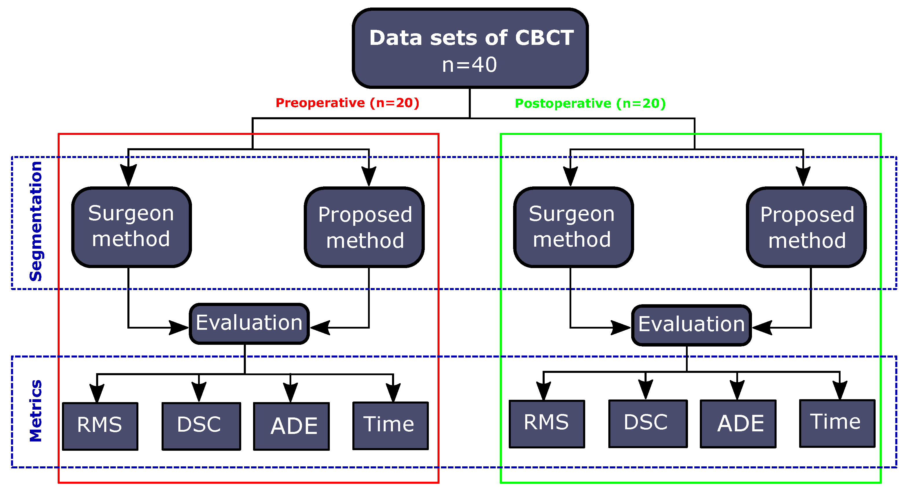
A retrospective study was performed by using 40 CBCT data sets from the database of the Simonas Grybauskas’ Orthognathic Surgery clinic. Before the study, all CBCT data sets were anonymised in order to protect the patients’ data. Half of them (n = 20) were preoperative (obtained one week before the surgery) and another half (n = 20) were postoperative (obtained about one week after surgery) scans of the same patients’ group. All scans were done using the i-CAT FLX V17 machine. All patients undertook double jaws correction. CBCT data sets were acquired with a resolution of an isotropic voxel of 0.3 mm, 230 mm × 170 mm field of view (FOV), the time of exposure was 7 s, tube voltage 120 kV and tube current 5 mA. Preoperative and postoperative CBCT data sets were segmented by an experienced oral and maxillofacial surgeon using ITK-SNAP software (Version 3.4.0) selecting a global threshold value for each case individually. Mandible and lower parts of skull (including maxilla, zygomatic bone) were used to perform the segmentation. Therefore, mentioned anatomical regions were selected as the segmentation target assessing the importance of them to perform a surgery. The study framework is presented in Figure 1.
2.2. Description of Proposed Method
The proposed method was based on the finding of an optimal threshold by using Otsu’s method in a sliding 3D window. However, Otsu’s method works most accurately when the analyzing histogram is bimodal. This means that the intensity values of voxels must be divided into two basic classes with intensity range [1, …, T] and with intensity range [T + 1, …, L] (where L is the upper limit of intensity in the volume), T representing the threshold optimally separating modes in bimodal histogram. The number of voxels with intensity threshold i is denoted by . A probability of intensity threshold i in an image is
N—the total number of voxels. Then, the probabilities that a randomly selected voxels belong to one of the classes or are
The average of classes is defined
The intensity average of the total image is defined by
Using discriminant analysis, Otsu’s method defines both classes variance of the thresholded image
Then the optimal threshold value is calculated by
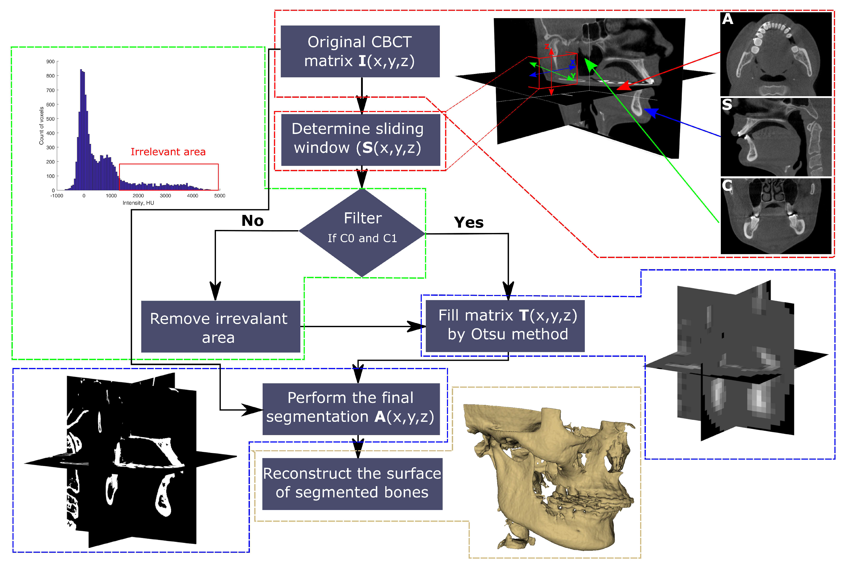
The illustration of the proposed method is presented in Figure 2.
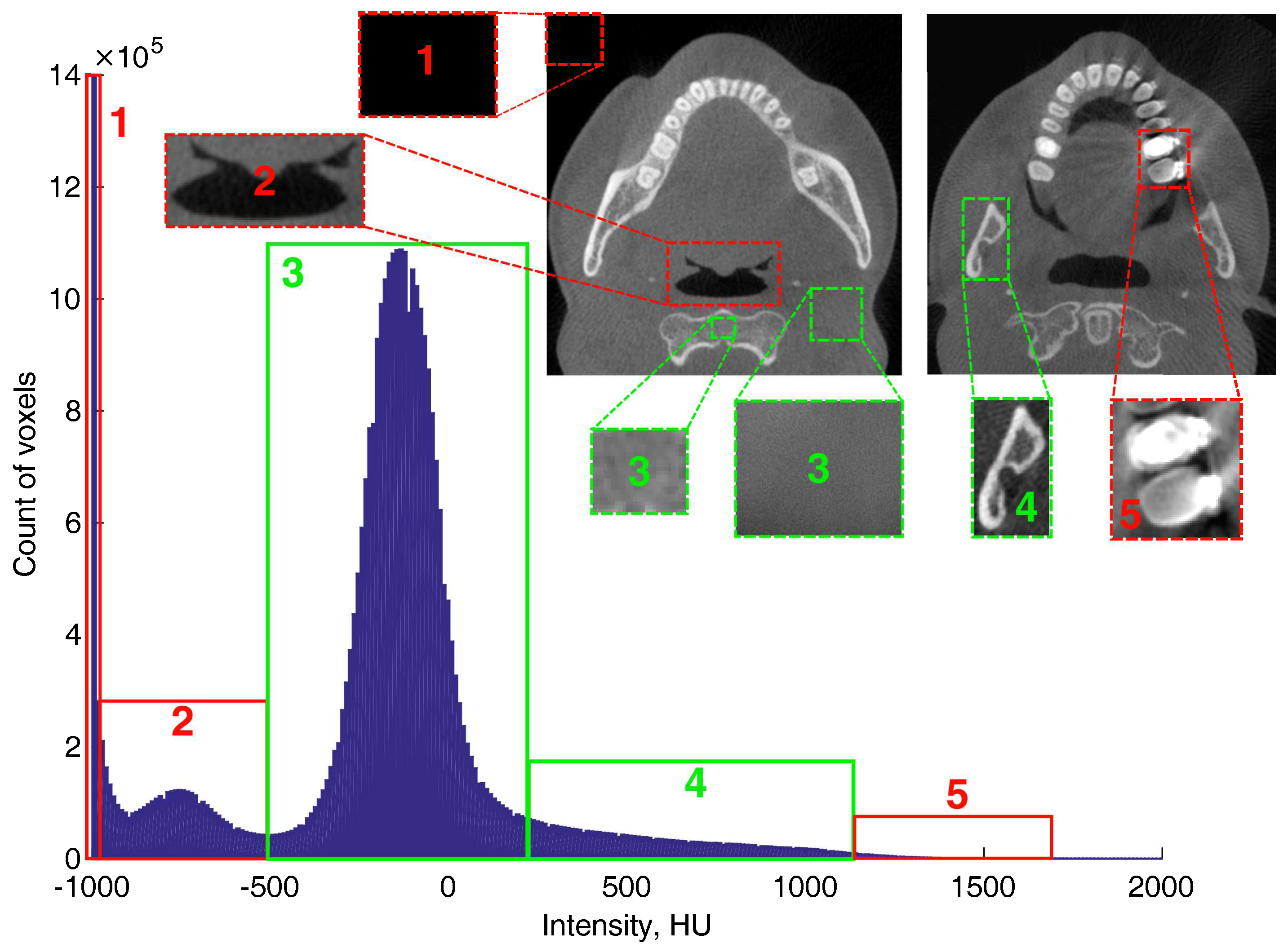
The typical histogram of CBCT data set is not bimodal and Otsu’s method does not work accurately in order to find optimal threshold value. The typical histogram of CBCT data set is presented in Figure 3.
In order to perform an accurate segmentation using Otsu’s method, a histogram filter was involved. The purpose of the filter is to remove irrelevant areas and to make analysed histograms bimodal. The optimal threshold was found after filtration, that is, removal of the , and areas in the histogram (Figure 3). Intensity values for histogram filtering areas were defined by the results of studies published in References [18,19]. Misch et al. [18] determined that the intensity of cortical bone of mandible is 1250 HU and it cover about 8% of the volume of mandible, trabecular bone intensity of mandible is 850–1250 HU, 350–850 HU levels corresponds to trabecular bone intensity of maxilla, levels of 150–350 HU limit posterior maxilla and levels of 150 HU could be found in sinus areas where the bone is very soft. The study performed by Norton et al. [19] divided the intensity scale of bone into these ranges of HU: anterior mandible 850 HU, posterior mandible/anterior maxilla 500–850 HU, posterior maxilla 0–500 HU, tuberosity region 0 HU. Air intensity is −1000 HU and internal anatomical areas such as cavity of maxillary sinuses, nasal cavities, airways are between −950 HU and −500 HU. This analysis was used to set which areas of the histogram are useful for the segmentation and which areas should be filtered out. Then the filter was built to automatically remove areas in the sliding volume histogram with the intensities of more than 1250 HU and areas with the intensities less than −500 HU. An optimal threshold value using Otsu’s method is found in the defined range [−500 HU ... 1250 HU]. The filter is involved before processing CBCT data set and it ensures that CBCT volumetric histogram is bimodal (Figure 4, C0—object, C1—background). Then the matrix of local thresholds (T(x,y,z)) is filled by the found T values and the final segmentation (A(x,y,z)) is performed by:
Here A(x,y,z)—3D final matrix of segmentation, I(x,y,z)—3D matrix of the original CBCT data set.
The local threshold value T is found in a volume of sliding window (S(x,y,z)), the segmentation object is the segment of bone (mandible and maxilla)—C0 and background is the segment of soft tissues (including soft bone)—C1 (Figure 4).
2.3. Surface Reconstruction
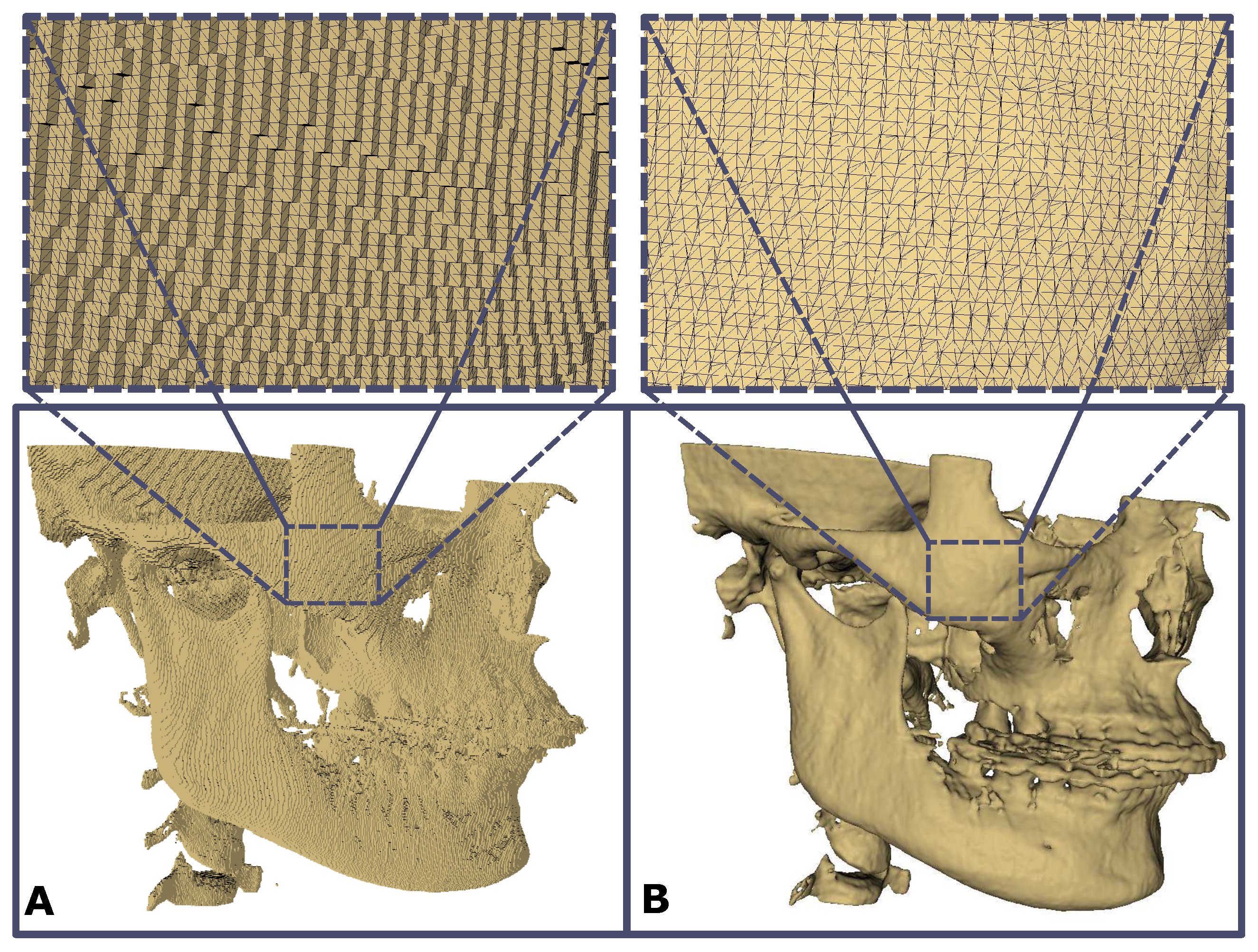
Segmented bone (A(x,y,z)) is saved as a surface in the STereoLithography (STL) file format. The reconstruction of the bone surface from segmented voxels is performed by the volumetric reconstruction algorithm (Visualization and Computer Graphics (VCG) reconstruction filter) using MeshLab software (Visual Computing Lab of ISTI–CNR, University of Pisa) [20,21] (Figure 5).
The basic parameters of the surface reconstruction ((1) voxel size, (2) the level of the subvolume reconstruction process, (3) geodesic weighting, number of Volume Laplacian iterations, (4) widening, (5) number of smoothing iterations) were used the same for all forty cases in order to have comparable results of reconstruction.
2.4. Evaluation of Method Accuracy
The results of the proposed algorithm were compared with the results of segmentation performed by an experienced surgeon. In order to evaluate the reliability of surgeon’s segmentation, the segmentations were done twice with a 2 weeks interval. For the quantitative evaluation of the reliability, Intraclass Correlation Coefficient (ICC) by using a two-way mixed model, unit: single rater and the type of relationship: absolute agreement method [22] was calculated by:
where = mean square for rows, k = number of raters/measurements; = mean square for error; = mean square for columns; n = number of subjects.
ICC was calculated separately for preoperative and postoperative cases and segmentation thresholds selected by the surgeon were used for this.
The evaluation of segmentation accuracy by using proposed method three basic metrics were used:
- (1)
- Root mean square (RMS) of the intersurface distance used to evaluate reconstructed surface mismatch:where represents the coordinates of reference surface point, —the coordinates of surface point created with the proposed method;
- (2)
- Dice similarity coefficient (DSC), used to evaluate volume discrepancy:where A represents the volume of the reference model, B—volume of automatically segmented bone;
- (3)
- Average intersurface distance error (ADE) was calculated by:where represents the coordinates of 3D point of the reference model, —the coordinates of 3D point of the automatically segmented model;
Positive and negative ADE values were calculated also.
Additional metric to evaluate the rapidity of segmentation the computation time of automatic segmentation was calculated. In this study, personal computer with parameters—processor—Intel(R) Core(TM) i7-4790 CPU @ 3.60 GHz, RAM—16 GB, system type—64-bit Windows 10 Operating System was used. The automatic method was implemented by using Matlab software.
3. Results
The reliability of segmentations performed by surgeon was evaluated by calculating ICC values for preoperative and postoperative CBCT data sets (Table 1).
The results show that in preoperative data ICC = 0.958 with 95% confidence interval [0.896 ... 0.983] and in postoperative data ICC = 0.931 with 95% confidence interval [0.836 ... 0.972]. Calculated values of ICC show that the level of surgeon reliability is sufficient [22].
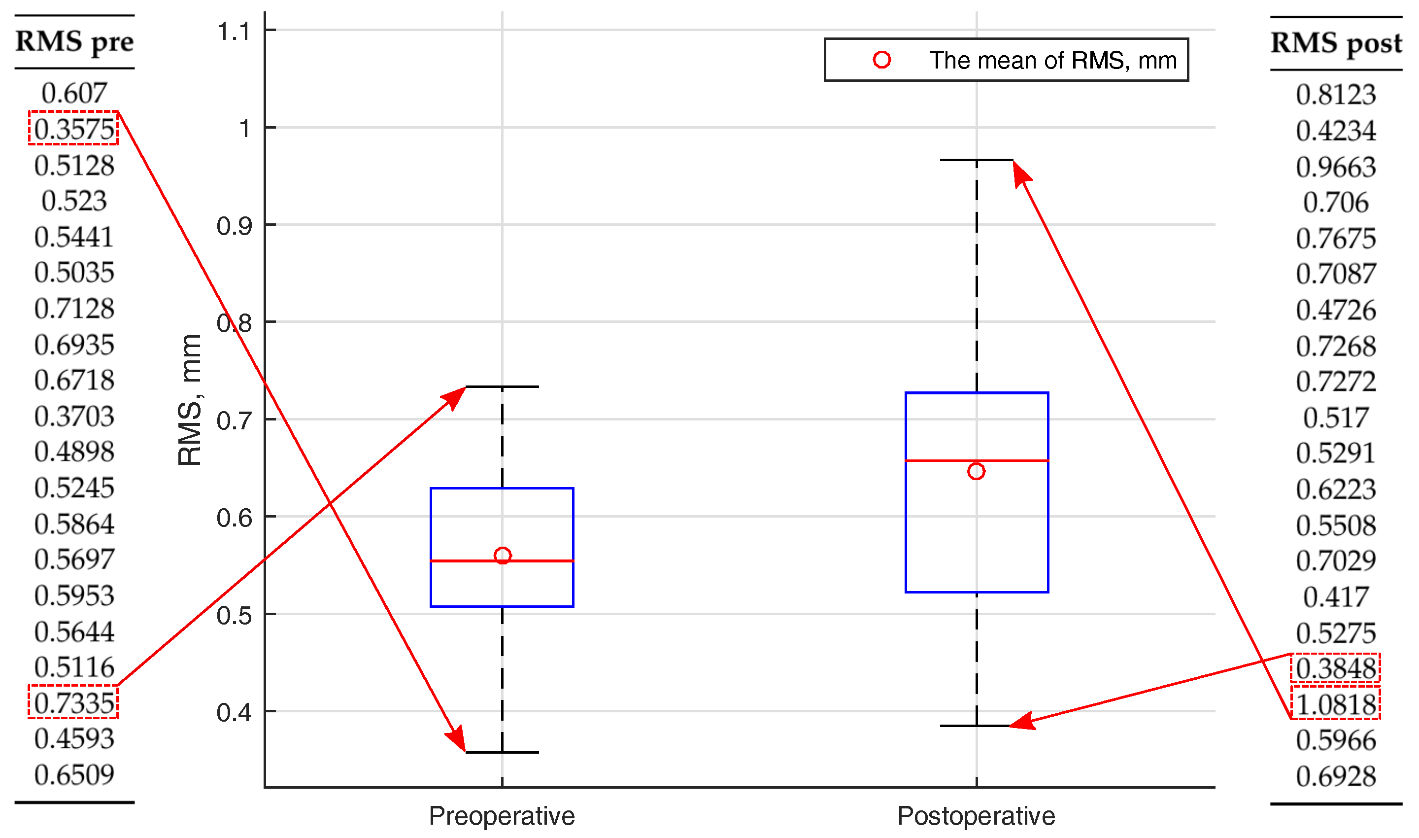
(1) The mean RMS value of intersurface distance in preoperative cases was 0.559 mm and in postoperative—0.647 mm. Calculated RMS values of intersurface distance for all cases are presented by a boxplot in Figure 6.
The interquartile range of boxplot is narrower for preoperative RMS values. The bigger distribution of RMS values is seen in postoperative cases. This could have been caused by a better quality of preoperative CBCT data sets.
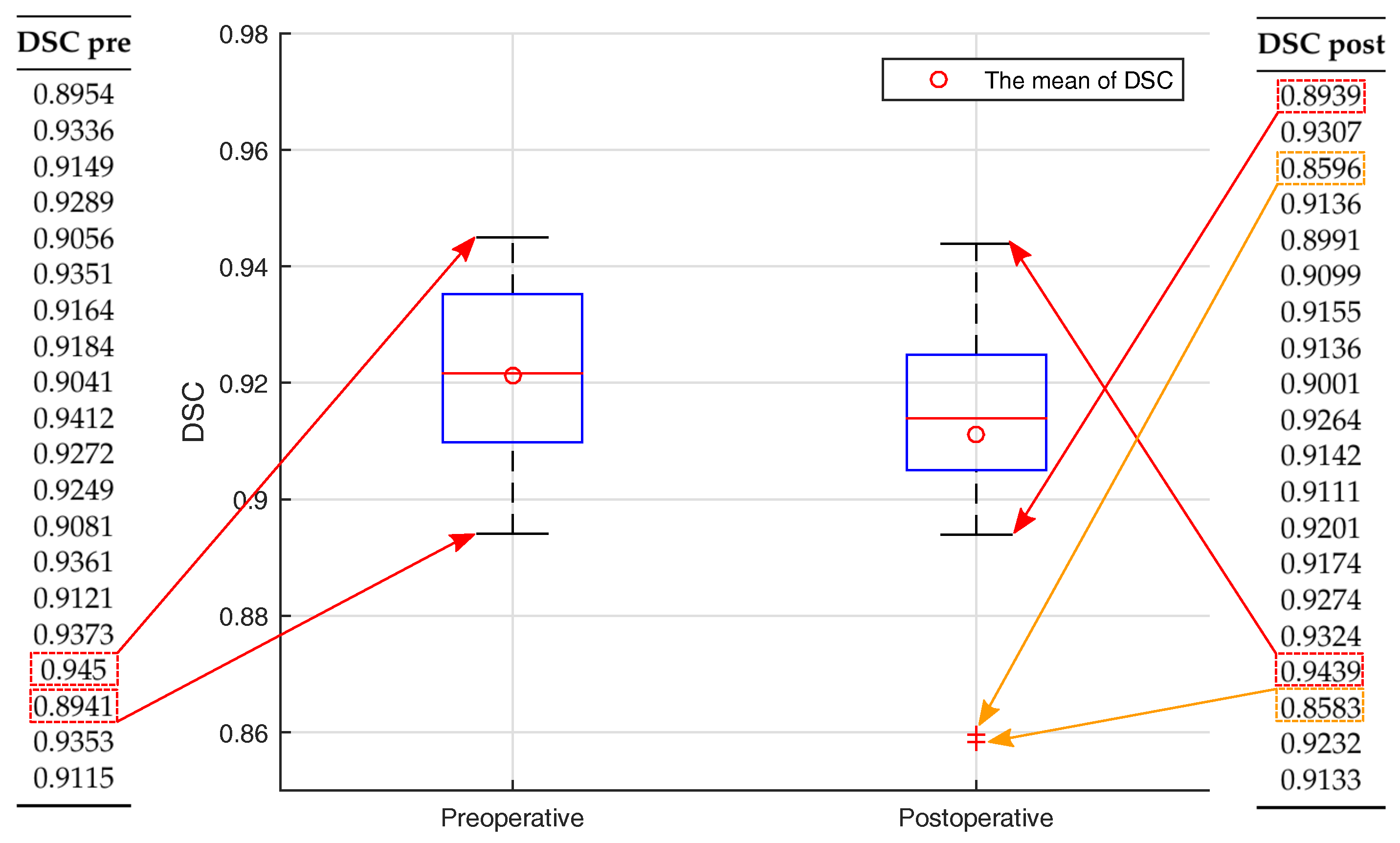
(2) The mean value of DSC was 0.921 in preoperative cases. In postoperative cases, the mean value of DSC was 0.911. Calculated DSC values are similar and are very high—more than 0.9. The results of DSC in preoperative and postoperative segmentation data are presented by using the boxplot function in Figure 7.
The narrower range of interquartile is found in postoperative cases. Two DSC values are out of the DSC range in postoperative cases and are marked as outliers.
(3) The ADE values were calculated and divided into three groups: general average, positive average and negative average. The whole results are presented in Table 2.
The mean value of computational time to perform an automatic segmentation by using all CBCT data sets was 46 s. Compared with other studies, this computation time is very fast. The achieved results are compared with the results of other similar studies. The comparison is presented in Table 2.
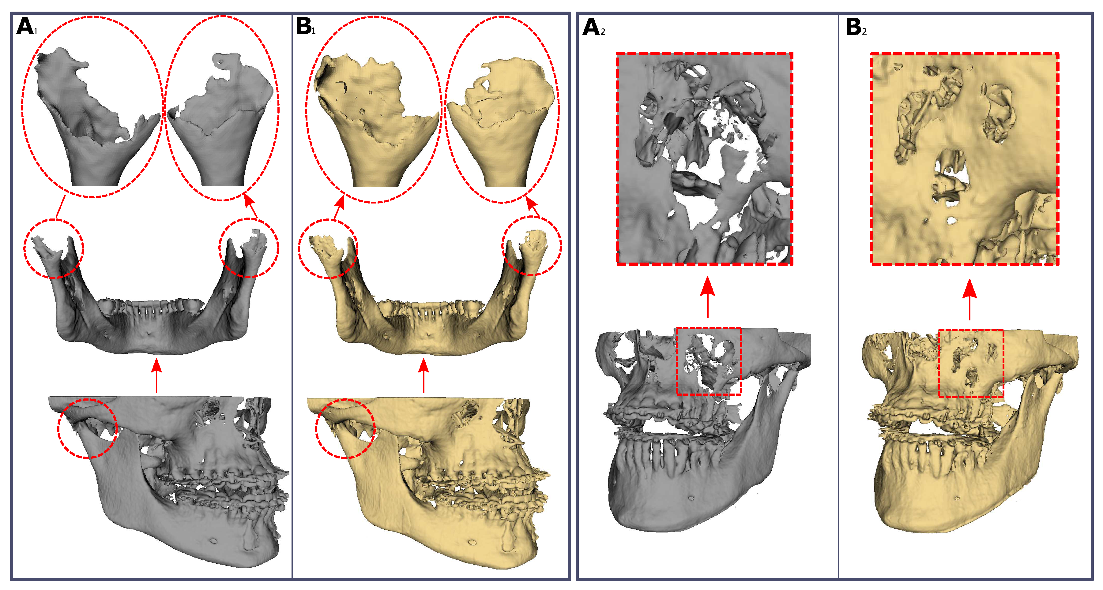
DSC is the most popular metric in order to prove the accuracy of segmentation. Achieved values of DSC were similar in comparison with other studies (values were near 0.9). ADE also is a frequent metric in order to evaluate the segmentation. In our study, ADE was calculated and divided into three groups. The results between ADE values in different groups (preoperative and postoperative) were compared. It was found that differences were similar (Table 2). In comparison with the other studies, in which the proposed method was used, ADE values were found lower. The proposed method showed a short computation time to an automatic segmentation performance. The comparison of segmentation results by using automatic and surgeon methods are shown in Figure 8.
The results of segmentation by using the proposed method showed that bones with low density were not fully segmented. However, areas of condyles and sinuses were segmented with fewer holes by using the proposed method, compared to the surgeon segmentation results (Figure 8).
4. Discussion
Automatic methods for bone segmentation are very important in order to get 3D surfaces. It helps surgeons in making correct diagnoses, in performing accurate and quicker VSP and in the evaluation of postoperative follow-up without the influence of surgeon’s experience [23,24,25,26,27]. The aim of this study was to evaluate method’s accuracy for bone segmentation in CBCT data sets. The method is based on the histogram filter, 3D sliding window and Otsu’s thresholding. The results of automatic segmentation revealed sufficient accuracy of bone segmentation. For the evaluation of method accuracy, three kind of metrics were used: voxel-based–DSC [15,17,28], based on the intersurface distance evaluation–RMS and ADE [16,17]. Additional metric based on the time to perform segmentation–computation time was calculated. The mean DSC coefficient values of two groups (preoperative and postoperative) were bigger than 0.9, which proved the complete overlap and high accuracy of the automatic and surgeon segmented bone voxels. The mean RMS values of intersurface distance for preoperative (0.559 mm) and postoperative (0.647 mm) cases were about two times bigger than the voxel size (0.3 mm). Calculated ADE values showed small discrepancies of surfaces. It shows that segmentation result is good, either we succeeded to avoid superimposition step because both automatic and global segmentations were made by using the same source data sets. In this way, surface superimposition did not yield any additional errors. Compared with the other studies [7,8,10], the proposed method performed the segmentation very rapidly ( 46 s/case). The achieved results showed that the proposed automatic method worked accurately.
However, the proposed method had some limitations. CBCT images were not filtered for metal artefacts (brackets, metal plates and mini-implants) before or after segmentation. Due to this reason, metal artefacts were seen in 3D models. These artefacts hide important areas of bone. Therefore, assessment of the bone near these artefacts became complicated and inaccurate. Especially it is important when postoperative follow-ups are performed [29,30]. The other limitation of the proposed method is the difficulty to segment areas with low density (thin anatomical areas, e.g., alveolar part of the mandible, mandibular condyles or areas of maxillary sinuses) in CBCT images [31]. This is also valid for other threshold-based segmentation methods. Problematic areas could be segmented including more sensitive techniques [31,32,33,34].
Further studies may be concentrated to evaluate proposed method with higher amount and different kind of CT/CBCT data sets. The next direction of further study may be to increase accuracy of the segmentation for anatomical areas with low density. Fully automatic segmentation of selected anatomical areas especially condyles would be important tool to increase the evaluation of treatment or postoperative follow-up [35,36].
5. Conclusions
The presented study proposed a new automatic method for bone segmentation in a CBCT data set. The important feature of the proposed segmentation method is simple and rapid implementation. The results of segmentation were very accurate and reliable to use in the clinical practice of oral and maxillofacial surgery. The method does not require access to a computer with high computation power parameters. It can be integrated into the most popular software of 3D medical imaging processing using an ordinary computer.
Author Contributions
All authors contributed equally to this work. All authors have read and agreed to the published version of the manuscript.
Funding
This research received no external funding.
Conflicts of Interest
The authors declare no conflict of interest.
Abbreviations
The following abbreviations are used in this manuscript:
| CBCT | Cone Beam Computed Tomography |
| 3D | Three dimensional |
| VSP | Virtual Surgical Plan |
| RMS | Root Mean Square |
| DSC | Dice Similarity Coefficient |
| ADE | Average Distance Error |
References
- Deeb, G.; Antonos, L.; Tack, S.; Carrico, C.; Laskin, D.; Deeb, J.G. Is Cone-Beam Computed Tomography Always Necessary for Dental Implant Placement? J. Oral Maxillofac. Surg. 2017, 75, 285–289. [Google Scholar] [CrossRef] [Green Version]
- Fourie, Z.; Damstra, J.; Schepers, R.H.; Gerrits, P.O.; Ren, Y. Segmentation process significantly influences the accuracy of 3D surface models derived from cone beam computed tomography. Eur. J. Radiol. 2012, 81, 524–530. [Google Scholar] [CrossRef]
- Pauwels, R.; Jacobs, R.; Singer, S.R.; Mupparapu, M. CBCT-based bone quality assessment: Are Hounsfield units applicable? Dentomaxillofac. Radio 2015, 44, 20140238. [Google Scholar] [CrossRef] [Green Version]
- Pauwels, R.; Nackaerts, O.; Bellaiche, N.; Stamatakis, H.; Tsiklakis, K.; Walker, A.; Bosmans, H.; Bogaerts, R.; Jacobs, R.; Horner, K. Variability of dental cone beam CT grey values for density estimations. Br. J. Radiol. 2013, 86, 20120135. [Google Scholar] [CrossRef] [Green Version]
- Katsumata, A.; Hirukawa, A.; Noujeim, M.; Okumura, S.; Naitoh, M.; Fujishita, M.; Ariji, E.; Langlais, R.P. Image artifact in dental cone-beam CT. Oral. Surg. Oral Med. Oral Pathol. Oral Radiol. Endod. 2006, 101, 652–657. [Google Scholar] [CrossRef]
- Wang, L.; Chen, K.C.; Shi, F.; Liao, S.; Li, G.; Gao, Y.; Shen, S.G.; Yan, J.; Lee, P.K.; Chow, B.; et al. Automated segmentation of CBCT image using spiral CT atlases and convex optimization. Med. Image Comput. Comput. Assist. Interv. 2013, 16, 251–258. [Google Scholar]
- Wang, L.; Chen, K.C.; Gao, Y.; Shi, F.; Liao, S.; Li, G.; Shen, S.G.; Yan, J.; Lee, P.K.; Chow, B.; et al. Automated bone segmentation from dental CBCT images using patch-based sparse representation and convex optimization. Med. Phys. 2014, 41, 043503. [Google Scholar] [CrossRef] [PubMed] [Green Version]
- Wang, L.; Gao, Y.; Shi, F.; Li, G.; Chen, K.C.; Tang, Z.; Xia, J.J.; Shen, D. Automated segmentation of dental CBCT image with prior-guided sequential random forests. Med. Phys. 2016, 43, 336–346. [Google Scholar] [CrossRef] [PubMed] [Green Version]
- Gollmer, S.T.; Buzug, T.M. Fully automatic shape constrained mandible segmentation from cone-beam CT data. In Proceedings of the 9th IEEE International Symposium on Biomedical Imaging (ISBI), Barcelona, Spain, 2–5 May 2012; pp. 1272–1275. [Google Scholar]
- Fan, Y.; Beare, R.; Matthews, H.; Schneider, P.; Kilpatrick, N.; Clement, J.; Claes, P.; Penington, A.; Adamson, C. Marker-based watershed transform method for fully automatic mandibular segmentation from cBct images. Dentomaxillofac. Radiol. 2019, 48, 20180261. [Google Scholar] [CrossRef] [PubMed]
- Van Eijnatten, M.; van Dijk, R.; Dobbe, J.; Streekstra, G.; Koivisto, J.; Wolff, J. CT image segmentation methods for bone used in medical additive manufacturing. Med. Eng. Phys. 2018, 51, 6–16. [Google Scholar] [CrossRef]
- Vaitiekunas, M.; Jegelevicius, D.; Sakalauskas, A.; Grybauskas, S. Method for automatic 3D bone segmentation in CBCT data. In Proceedings of the Joint Conference of the European Medical and Biological Engineering Conference (EMBEC) and the Nordic-Baltic Conference on Biomedical Engineering and Medical Physics (NBC), Tampere, Finland, 11–15 June 2017; pp. 1–4. [Google Scholar]
- Otsu, N. A Threshold Selection Method from Gray-Level Histograms. IEEE Trans. Syst. Man Cybern. 1979, 9, 62–66. [Google Scholar] [CrossRef] [Green Version]
- Yang, P.; Clapworthy, G.; Dong, F.; Codreanu, V.; Williams, D.; Liu, B.; Roerdink, J.B.; Deng, Z. GSWO: A programming model for GPU-enabled parallelization of sliding window operations in image processing. Signal Process. Image Commun. 2016, 47, 332–345. [Google Scholar] [CrossRef] [Green Version]
- Dice, L.R. Measures of the Amount of Ecologic Association Between Species. Ecology 1945, 26, 297–302. [Google Scholar] [CrossRef]
- Park, G.H.; Son, K.B.D.; Lee, K.B. Feasibility of using an intraoral scanner for a complete-arch digital scan. J. Prosthet. Dent. 2019, 121, 803–810. [Google Scholar] [CrossRef] [PubMed]
- Hosseini, M.P.; Nazem-Zadeh, M.R.; Pompili, D.; Jafari-Khouzani, K.; Elisevich, K.; Soltanian-Zadeh, H. Comparative performance evaluation of automated segmentation methods of hippocampus from magnetic resonance images of temporal lobe epilepsy patients. Med. Phys. 2016, 43, 538–553. [Google Scholar] [CrossRef]
- Misch, C.E. Density of bone: effect on treatment plans, surgical approach, healing, and progressive boen loading. Int. J. Oral Implantol. 1990, 6, 23–31. [Google Scholar]
- Norton, M.R.; Gamble, C. Bone classification: an objective scale of bone density using the computerized tomography scan. Clin. Oral Implants Res. 2001, 12, 79–84. [Google Scholar] [CrossRef]
- Meshlab Software. Available online: www.meshlab.net (accessed on 5 May 2019).
- Curless, B.; Levoy, M. A volumetric method for building complex models from range images. In Proceedings of the 23rd Annual Conference on Computer Graphics and Interactive Techniques—SIGGRAPH ’96, New York, NY, USA, 11–15 June 1996; pp. 303–312. [Google Scholar]
- Koo, T.K.; Li, M.Y. A Guideline of Selecting and Reporting Intraclass Correlation Coefficients for Reliability Research. J. Chiropr. Med. 2016, 15, 155–163. [Google Scholar] [CrossRef] [Green Version]
- Wallner, J.; Hochegger, K.; Chen, X.; Mischak, I.; Reinbacher, K.; Pau, M.; Zrnc, T.; Schwenzer-Zimmerer, K.; Zemann, W.; Schmalstieg, D.; et al. Clinical evaluation of semi-automatic open-source algorithmic software segmentation of the mandibular bone: Practical feasibility and assessment of a new course of action. PLoS ONE 2018, 13, e0196378. [Google Scholar] [CrossRef]
- Lebre, M.A.; Vacavant, A.; Grand-Brochier, M.; Rositi, H.; Abergel, A.; Chabrot, P.; Magnin, B. Automatic segmentation methods for liver and hepatic vessels from CT and MRI volumes, applied to the Couinaud scheme. Comput. Biol. Med. 2019, 110, 42–51. [Google Scholar] [CrossRef]
- Sakinis, T.; Milletari, F.; Roth, H.; Korfiatis, P.; Kostandy, P.; Philbrick, K.; Akkus, Z.; Xu, Z.; Xu, D.; Erickson, B.J. Interactive segmentation of medical images through fully convolutional neural networks. arXiv 2019, arXiv:1903.08205. [Google Scholar]
- Fripp, J.; Crozier, S.; Warfield, S.K.; Ourselin, S. Automatic segmentation of the bone and extraction of the bone-cartilage interface from magnetic resonance images of the knee. Phys. Med. Biol. 2007, 52, 1617–1631. [Google Scholar] [CrossRef] [PubMed]
- Indraswari, R.; Arifin, A.Z.; Suciati, N.; Astuti, E.R.; Kurita, T. Automatic segmentation of mandibular cortical bone on cone-beam CT images based on histogram thresholding and polynomial fitting. Int. J. Intell. Eng. Syst. 2019, 12, 130–141. [Google Scholar] [CrossRef]
- Taha, A.A.; Hanbury, A. Metrics for evaluating 3D medical image segmentation: Analysis, selection, and tool. BMC Med. Imaging 2015, 15, 29. [Google Scholar] [CrossRef] [PubMed] [Green Version]
- Shokri, A.; Jamalpour, M.R.; Khavid, A.; Mohseni, Z.; Sadeghi, M. Effect of exposure parameters of cone beam computed tomography on metal artifact reduction around the dental implants in various bone densities. BMC Med. Imaging 2019, 19, 34. [Google Scholar] [CrossRef]
- Scarfe, W.C.; Farman, A.G.; Sukovic, P. Clinical applications of cone-beam computed tomography in dental practice. J. Can. Dent. Assoc. 2006, 72, 75–80. [Google Scholar]
- Chang, Y.B.; Xia, J.J.; Yuan, P.; Kuo, T.H.; Xiong, Z.; Gateno, J.; Zhou, X. 3D segmentation of maxilla in cone-beam computed tomography imaging using base invariant wavelet active shape model on customized two-manifold topology. J. Xray Sci. Technol. 2013, 21, 251–282. [Google Scholar] [CrossRef] [Green Version]
- Xi, T.; Schreurs, R.; Heerink, W.J.; Bergé, S.J.; Maal, T.J. A novel region-growing based semi-automatic segmentation protocol for three-dimensional condylar reconstruction using cone beam computed tomography (CBCT). PLoS ONE 2014, 9, e111126. [Google Scholar] [CrossRef]
- Descoteaux, M.; Audette, M.; Chinzei, K.; Siddiqi, K. Bone enhancement filtering: application to sinus bone segmentation and simulation of pituitary surgery. Comput. Aided Surg. 2006, 11, 247–255. [Google Scholar] [CrossRef]
- Chuang, Y.J.; Doherty, B.M.; Adluru, N.; Chung, M.K.; Vorperian, H.K. A Novel Registration-Based Semiautomatic Mandible Segmentation Pipeline Using Computed Tomography Images to Study Mandibular Development. J. Comput. Assist. Tomogr. 2018, 42, 306–316. [Google Scholar] [CrossRef]
- Engelbrecht, W.P.; Fourie, Z.; Damstra, J.; Gerrits, P.O.; Ren, Y. The influence of the segmentation process on 3D measurements from cone beam computed tomography-derived surface models. Clin. Oral Investig. 2013, 17, 1919–1927. [Google Scholar] [CrossRef] [PubMed]
- Nicolielo, L.F.P.; Van Dessel, J.; Shaheen, E.; Letelier, C.; Codari, M.; Politis, C.; Lambrichts, I.; Jacobs, R. Validation of a novel imaging approach using multi-slice CT and cone-beam CT to follow-up on condylar remodeling after bimaxillary surgery. Int. J. Oral Sci. 2017, 9, 139–144. [Google Scholar] [CrossRef] [PubMed] [Green Version]
Figure 1.
The framework of the current study. The study was performed using preoperative and postoperative Cone Beam Computed Tomography (CBCT) data sets. Four metrics (Root Mean Square (RMS), Dice Similarity Coefficient (DSC), Average Distance Error (ADE) and Time) were used to evaluate the proposed method.

Figure 2.
Implementation of segmentation by using the proposed automatic method.

Figure 3.
Typical histogram of CBCT data set. The basic areas: air (1), internal anatomical structures containing air (2), soft tissues/soft bone (3), bone (4) and metal artifacts/restorative materials (5).
Figure 3.
Typical histogram of CBCT data set. The basic areas: air (1), internal anatomical structures containing air (2), soft tissues/soft bone (3), bone (4) and metal artifacts/restorative materials (5).

Figure 4.
Analysing histogram (2) in selected sliding window volume (1) in order to find an optimal threshold T to segmented a bone (3).
Figure 4.
Analysing histogram (2) in selected sliding window volume (1) in order to find an optimal threshold T to segmented a bone (3).

Figure 5.
Reconstruction of segmented bone. (A) The surface of the bone after segmentation, (B) Reconstructed surface of the bone. At the top, are shown the small fragments of surfaces before and after reconstruction.
Figure 5.
Reconstruction of segmented bone. (A) The surface of the bone after segmentation, (B) Reconstructed surface of the bone. At the top, are shown the small fragments of surfaces before and after reconstruction.

Figure 6.
Distributions of RMS values of preoperative and postoperative segmentation data.

Figure 7.
Distribution of DSC values of preoperative and postoperative segmentation data.

Figure 8.
Evaluation of two random selected 3D models using different segmentation methods. (A) represents 3D models segmented using a global threshold method by the surgeon, (B)—segmented with proposed method (region of interest: 1–condyles, 2–sinuses).
Figure 8.
Evaluation of two random selected 3D models using different segmentation methods. (A) represents 3D models segmented using a global threshold method by the surgeon, (B)—segmented with proposed method (region of interest: 1–condyles, 2–sinuses).


Table 1.
Results of Intraclass Correlation Coefficient (ICC) using single rater, absolute agreement and 2-way random effects model.
Table 1.
Results of Intraclass Correlation Coefficient (ICC) using single rater, absolute agreement and 2-way random effects model.
| Itraclass Correlation | 95% Confidence Interval | F Test with True Value 0 | |||||
|---|---|---|---|---|---|---|---|
| Lower Bound | Upper Bound | Value | df1 | df2 | Sig | ||
| Single measures preoperative | 0.958 | 0.896 | 0.983 | 49.03 | 19 | 19 | 0.000 |
| Single measures postoperative | 0.931 | 0.836 | 0.972 | 27.43 | 19 | 19 | 0.000 |
© 2019 by the authors. Licensee MDPI, Basel, Switzerland. This article is an open access article distributed under the terms and conditions of the Creative Commons Attribution (CC BY) license (http://creativecommons.org/licenses/by/4.0/).
Share and Cite
MDPI and ACS Style
Vaitiekūnas, M.; Jegelevičius, D.; Sakalauskas, A.; Grybauskas, S. Automatic Method for Bone Segmentation in Cone Beam Computed Tomography Data Set. Appl. Sci. 2020, 10, 236. https://doi.org/10.3390/app10010236
AMA Style
Vaitiekūnas M, Jegelevičius D, Sakalauskas A, Grybauskas S. Automatic Method for Bone Segmentation in Cone Beam Computed Tomography Data Set. Applied Sciences. 2020; 10(1):236. https://doi.org/10.3390/app10010236
Chicago/Turabian StyleVaitiekūnas, Mantas, Darius Jegelevičius, Andrius Sakalauskas, and Simonas Grybauskas. 2020. "Automatic Method for Bone Segmentation in Cone Beam Computed Tomography Data Set" Applied Sciences 10, no. 1: 236. https://doi.org/10.3390/app10010236
Note that from the first issue of 2016, this journal uses article numbers instead of page numbers. See further details here.