
Crop Sequencing to Improve Productivity and Profitability in Irrigated Double Cropping Using Agricultural System Simulation Modelling


1
School of Agricultural, Environmental and Veterinary Sciences, Charles Sturt University, Wagga Wagga, NSW 2650, Australia
2
Gulbali Institute for Agriculture, Water and Environment, Charles Sturt University, Wagga Wagga, NSW 2650, Australia
*
Author to whom correspondence should be addressed.
Agronomy 2022, 12(5), 1229; https://doi.org/10.3390/agronomy12051229
Submission received: 30 April 2022
/
Revised: 17 May 2022
/
Accepted: 18 May 2022
/
Published: 20 May 2022
(This article belongs to the Special Issue Optimal Water Management and Sustainability in Irrigated Agriculture)
Abstract
:Land and water are two major inputs for crop production. Simulation modelling was used to determine crop sequences that maximise farm return. Crop yield was determined for different irrigation scheduling scenarios based on the fraction of available soil water (FASW). Farm returns ($ ML−1 and $ ha−1) were evaluated for seven crop sequences. Three irrigation water price scenarios (dry, median, wet) were considered. The yield of summer crops increased with irrigation. For winter crops, despite increase in irrigation, the yield would not increase. The optimum irrigation (ML ha−1) was: soybean 8.2, maize 10.4, wheat 2.5, barley 3.1, fababean 2.5, and canola 2.7. The water productivity curve of summer crops has a parabolic shape, increasing with FASW, reaching a maximum value at FASW 0.4–0.6, and then decreasing. The water productivity of winter crops decreases as FASW increases following a power function. Gross margins are positive when water is cheap ($60 ML−1) and when water has a median price ($124 ML−1). When water is expensive ($440 ML−1), positive gross margin would be obtained only for the continuous wheat scenario. Deficit irrigation of summer crops leads to significant yield loss. Supplemental irrigation of winter crops results in the highest gross margin per unit of water.
1. Introduction
The rapid growth of the world population and pressure on land and environmental resources has amplified the need to increase food and fibre production with minimal resource input. Multiple cropping or increasing cropping intensity is one means of increasing global crop production [1]. Crop diversification increases food production sustainability by supressing pests, absorbing climatic shocks, reducing fertiliser use, and reducing business risks [2]. In the Australian grain crop production system, winter crops are normally grown under a dryland/rainfed environment. When and where water is available, supplemental irrigation is applied as pre-irrigation in autumn and at the reproductive growth stage in spring. However, with the changing climate and competing needs such as environmental watering requirements, the amount of water available for irrigation is declining. In the Riverina region of south-eastern New South Wales (NSW), the farm-land holdings are also relatively small compared to other parts of the country. As a result, there is a need to optimise the limited amount of available irrigation water and land resources.
Irrigation farmers in the region have water entitlements, which are an ongoing share of surface and ground water resources in their catchment. However, they do not always obtain 100% of their entitlement as this depends on the rainfall in the season and water already available in the dams. Depending on the reliability of obtaining the full amount of entitlement, there are two kinds of water securities: high security water and general security water. High security water entitlement holders obtain 100% of their entitlement unless there is severe drought. This is the water for permanent plantings such as horticulture and viticulture. General security water is for annual crops. Most of the water in the region is as general security entitlement. When there is low or no general security water allocated, farmers buy water on the water market. The price of water varies from year to year depending on the amount of water available in the dams and the prevailing rainfall. As a result, the gross margin per unit of irrigation water also varies with the price of water.
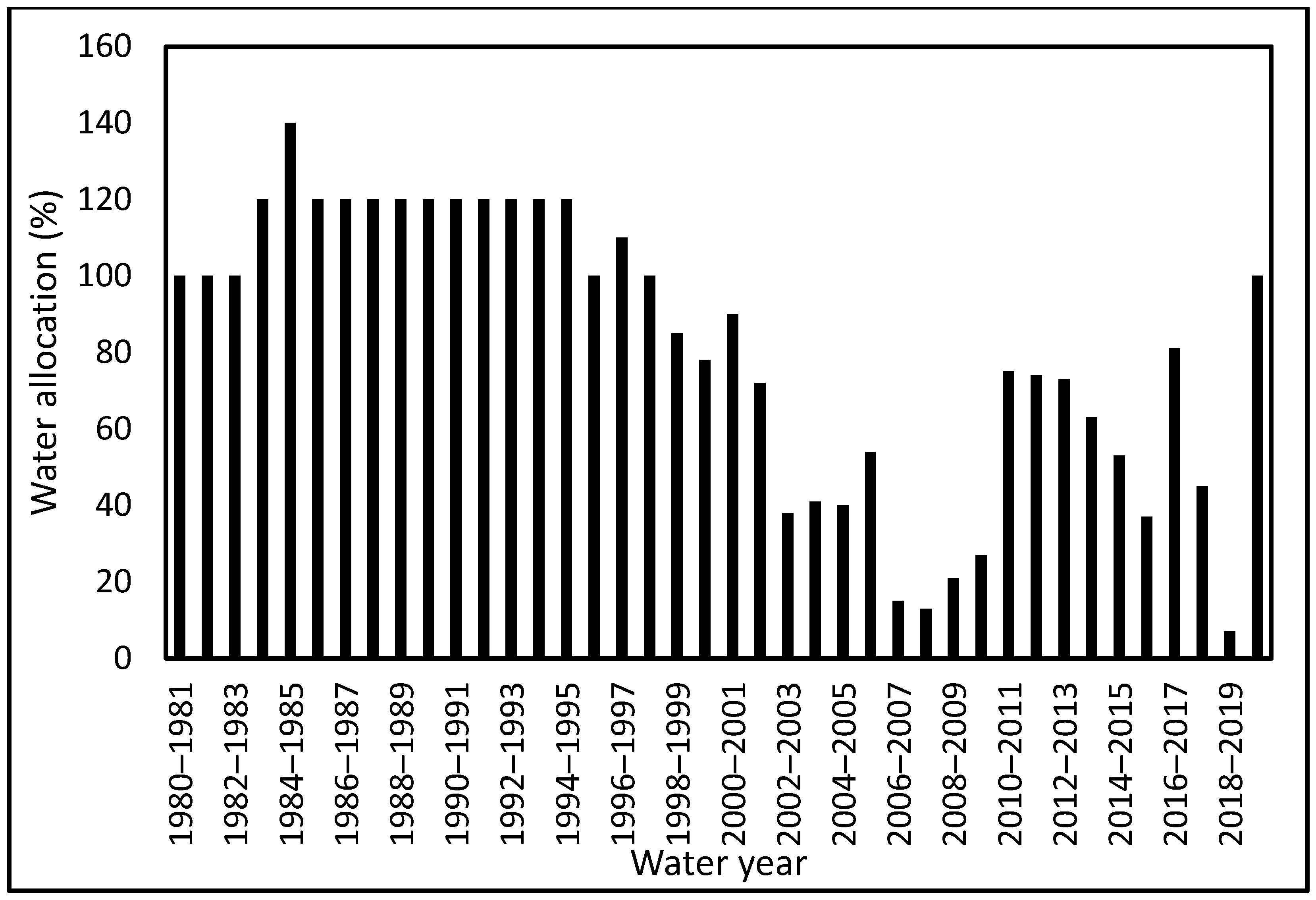
In recent years, low water allocation brought about by a combination of climatic and environmental policy-related factors have constrained Riverina irrigators’ production capacity. In the past 20 years, the amount of water in the region has been around 40% less than the long-term average (Figure 1). As a result, average seasonal allocations were less than 50% of the entitlement with high year to year variability. Innovative on-farm water management practices and planning are required to maintain a profitable irrigation industry in a future climate of reduced and variable irrigation water supply [3]. Some of the approaches that could help farmers adapt to reduced water allocations by increasing water and land productivity are: partial (deficit) irrigation, changes in crop rotations, crop species or varieties, and changes in water allocation to winter crops relative to summer crops [4,5,6]. In this study, different winter–summer crop sequences were evaluated in terms of gross margin per unit of water applied and per unit of cultivated land area. Crop yields were simulated using Agricultural Production Systems sIMulator (APSIM v.7.10) [7].
2. Materials and Method
2.1. General Description of the Study Area
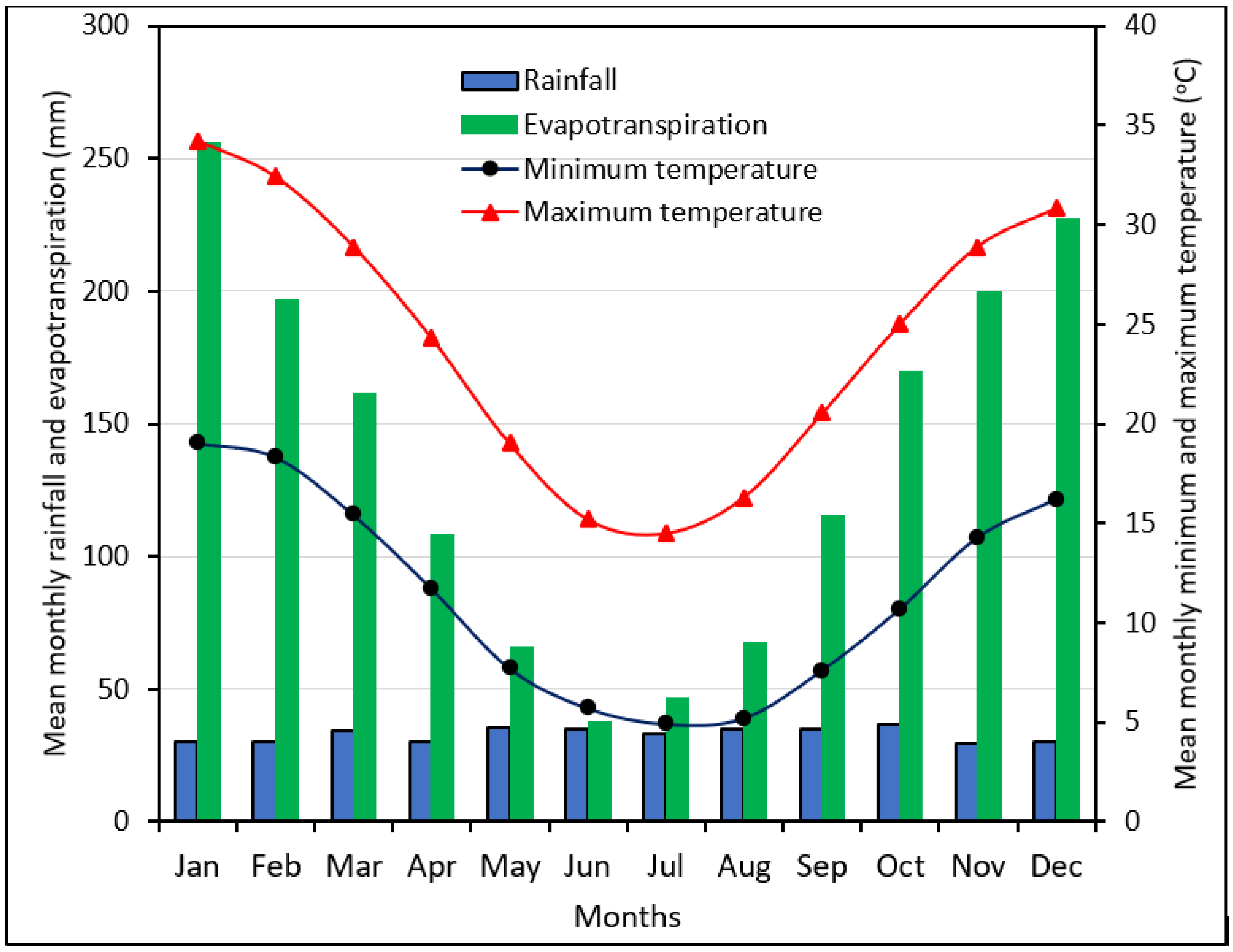
The study area is at Leeton in the Riverina region in NSW, Australia. The Riverina region of southern NSW has a mixed (crop and livestock) farming system. There are two large irrigation areas, Murrumbidgee and Coleambally, in the region. The Murrumbidgee river, the third longest in the country, originates from two large dams, Blowering and Burrinjuck, in the Snowy mountain of the Great Dividing Range. Water is diverted to the two irrigation areas using the two weirs, Berembed and Gogeldrie, on the Murrumbidgee river. The major irrigated crops in the region are horticulture, grapevine, cotton, rice, legumes, and maize. The climate of the region (south-eastern NSW) is partly semi-arid and partly temperate. It has a cold winter and hot summer with monthly temperature variation shown in Figure 2.
The annual mean minimum temperature is 11 °C while the mean maximum temperature is 24 °C. It has high evapotranspiration except during the winter season. The mean annual rainfall is 395 mm (monthly average 33 mm) and mean annual evapotranspiration is 1652 mm (http://www.bom.gov.au/ (accessed on 14 September 2021)).
2.2. Crops Used in the Study
Two summer crops (maize and soybean) and four winter crops (barley, canola, fababean, and wheat) commonly grown in the Australian wheat-belt were chosen for this study. In the Riverina region, in the summer season, after the winter crop harvest, fields are either left fallow or sown to a summer crop (double-cropping), depending on irrigation water availability. Introduction of summer crops in a winter-dominant cropping system is important for farming system sustainability to manage diseases and weeds. However, determining the crop sequence or which crop follows which requires careful planning. When double cropping is used, the time of harvest of one crop may overlap with the time of sowing of the next crop. Careful planning and choice of variety is required to ensure smooth transition. The availability of short-season varieties in recent years has enabled timely sowing of a crop and harvest without incurring substantial yield penalty. In order to meet crop water demand during the critical reproductive growth stages of crop development, where possible, supplemental irrigation of winter crops is used [8].
In the region, maize (Zea mays L.) is grown for silage and grain production. Depending on the variety, the length of growing season from planting to harvest is 130 to 150 days. The average maize irrigation requirement is 8–9 ML ha−1 with an average grain yield of 10.2 t ha−1 [9]. In southern NSW, the optimum time of sowing of maize is from early October to mid-November. Riverina is one of the two areas where soybean is widely grown in NSW. The soybean (Glycine max L.) irrigation requirement is 6–8 ML ha−1. Its optimum sowing time is mid-November to mid-December. For barley (Hordeum vulgare L.), sowing time is important to avoid risk of frost damage and drought stress during and after anthesis [10]. Its recommended sowing time is from mid-May to mid-June. Canola (Brassica napus L.) is a profitable break crop for weed and disease control. Its best sowing time is from the fourth week of April to the second week of May. Fababeans (Vicia faba L.) is an important break crop in crop rotation for disease control and nitrogen fixation [11]. The recommended sowing window is from the fourth week of April to the second week of May [12]. The optimum sowing time of wheat (Triticum aestivum L.) is not fixed but varies with location, season and variety [13]. Supplemental irrigation is used for winter crops during critical growth stages [14].
2.3. Simulation Setup
2.3.1. Weather and Soil Data
The Agricultural Production Systems sIMulator (APSIM) version 7.10 was used to simulate water-limited potential yield of the crops [7]. The details of the model can be found at www.apsim.info (accessed on 4 August 2021). Briefly, APSIM links the specific crop module (CROP), the soil water module (SOILWAT), the nitrogen module (SOILN), and residue module (RESIDUE) and irrigation. The model calculates biomass accumulation from solar radiation interception and adjusts for water and nitrogen stresses. Empirical coefficients are used to partition the biomass into different organs. The model can be used to study the effect of environmental factors and management decisions on resource use, crop growth, and yield. APSIM requires climate, soil, crop, and management decisions’ data to simulate crop yield. The SILO patched point daily climate dataset (1989–2020) of the Yanco Agricultural Institute Station (−34.6222° latitude and 146.4326° longitude) was used ([15], https://legacy.longpaddock.qld.gov.au/silo/ (accessed on 23 July 2021)). The soil of the study area is Brown Chromosol with a moderate water holding capacity (126 mm/m), the hydrologic characteristics of which, as used in APSIM, are shown in Table 1 [16]. The APSIM model has already been calibrated and validated for the crops used in this study: wheat [17,18], soybean [19], fababean [20,21], maize [22], barley [23], and canola [24,25].
2.3.2. Crop Sequences
Seven winter–summer crop sequences were evaluated under different water allocation/water price scenarios and irrigation amounts (Table 2). These were selected and adapted based on Napier et al. [26]. The simulation was done for five seasons (three winter and two summer—starting with winter season and ending with winter season). Crop cultivars and sowing dates used in the APSIM simulation were: soybean (cv. dragon), 15 Nov; maize (generic—early maturing), 15 Nov; fababean (cv. fiord), 15 May; wheat (cv. suntop), 01 May; barley (cv. scope), 15 May; canola (generic—early), 01 May. The soil water, nitrogen and organic matter were reset at the time of sowing in the long-term simulations.
2.3.3. Soil Water Deficit
Irrigation would be applied when the soil moisture is at a certain fraction of available soil water, hereafter designated as FASW. FASW varies between 0 and 1: 1 when the soil water is close to field capacity or drained upper limit and 0 when the soil water is close to permanent wilting point or drained lower limit. FASW is computed as:
where FASW = fraction of available soil water (0–1); θ = soil water content (cm3 cm−3); DUL = drained upper limit or field capacity (cm3 cm−3); LL15 = soil water content ((cm3 cm−3) at wilting point or 1.5 MPa soil water potential). In this study, irrigation scheduling at the following FASWs was investigated: 0.1, 0.2, 0.3, 0.4, 0.5, 0.6, 0.7, 0.8, and 0.9. For example, FASW 0.1 means irrigation is applied when the moisture remaining in the soil is 10% of the available soil water. This is a dry scenario, which means the crop is under water stress. On the other hand, in FASW 0.9, irrigation is applied while the soil moisture is still 90% of full capacity (a wet scenario). For all crop sequence scenarios and soil moisture deficit levels, the variations in the total seasonal irrigation, crop yield, and water productivity were determined.
Gross margins ($ ML−1 and $ ha−1) were determined for different winter–summer crop sequences, irrigation water price scenarios, and soil moisture deficit levels. Irrigation scheduling is determined by the amount of water available in the soil and the rate at which the crop uses this water. For most crops, crop yield is not affected if irrigation is applied before 50% of the available soil moisture (FASW 0.5) is depleted. For gross margin analysis, three soil moisture deficit scenarios were considered. In the first scenario, irrigation would be applied when the soil water is depleted to 20% of the available water (FASW 0.2) (dry scenario). The other scenarios are FASW 0.5 (medium scenario) and FASW 0.8 (wet scenario). The furrow irrigation water application efficiency was set at 75%.
2.4. Water Allocation Scenarios
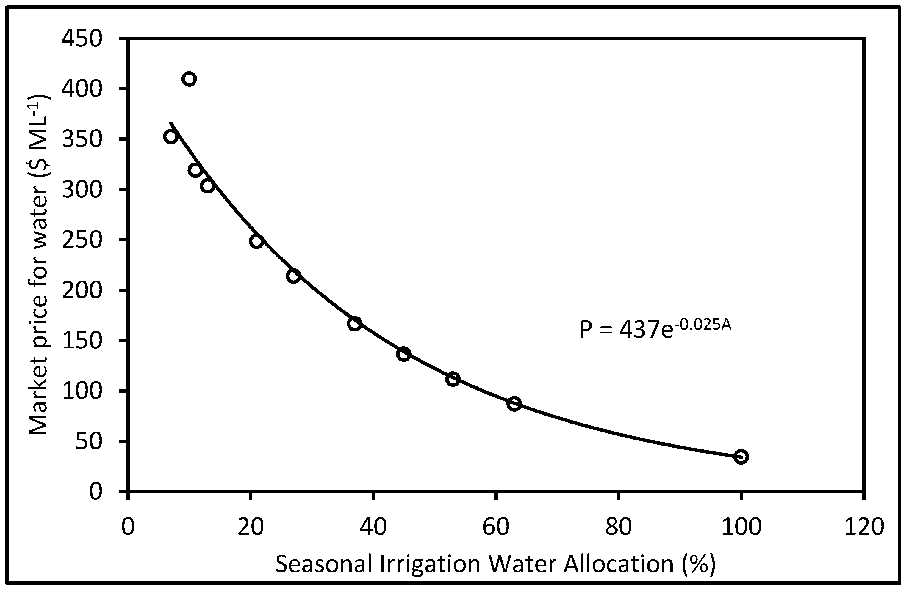
Water price highly varies from year to year depending on dam storage and rainfall in the catchments. As a result, the gross margin was determined for different percentiles of water price obtained from historical water allocation prices of the Murrumbidgee river catchment (https://www.awe.gov.au/abares/research-topics/water/water-market-outlook (accessed on 24 August 2021)). The 25 percentile irrigation water price was $60 ML−1, the median (50 percentile) irrigation water price was $124 ML−1, and the 75 percentile irrigation water price was $440 ML−1. The annual average water prices for different water-years were as shown in Figure 3. The generalized price-allocation function is shown in Equation (2):
where P is the market water price ($ ML−1); A is the seasonal allocation (%). A similar relationship was reported by [3].
P = 437 × e−0.025A
2.5. Gross Margin Analysis
Gross margin was calculated using the Decision Support Tool developed during the “Correct Crop Sequencing” Grain Research and Development Cooperation (GRDC) project (https://www.dpi.nsw.gov.au/agriculture/budgets/costs/cost-calculators/correct-crop-sequencing-decision-support-tool (accessed on 25 September 2021)).
Gross margin for a given cropping season was calculated as:
Gross margin ($ ha−1) = Gross income ($ ha−1) − Variable cost ($ ha−1)
Gross income ($ ha−1) = Grain yield (t ha−1) * Price ($ t−1)
Variable cost ($ ha−1) = Cost of water ($ ha−1) + Cost of other inputs and farm operations (cultivation, sowing, fertiliser, spraying, harvest) ($ ha−1)
Cost of water ($ ha−1) = Water use (ML ha−1) * Water price ($ ML−1)
Gross margin per unit of water ($ ML−1) = Gross margin ($ ha−1)/Water use (ML ha−1)
The data required to run this model are grain yield, grain yield price, water use, cost of water, and costs related to other farm operations (cultivation, sowing, fertiliser, spraying, harvest). It calculates gross margins per unit area ($ ha−1) and per unit of water ($ ML−1) for different crop sequences. The default variable cost (excluding cost of water) used in the decision support tool was adopted for this simulation study as it is from the same site as this simulation study. The variation of the variables costs over time were not considered. The long-term average price for the Riverina area, as obtained from Grain Price Australia Listings igrainPlus (https://www.igrain.com.au/) (accessed on 14 August 2021) was used in the Gross Margin Decision Support Tool. Accordingly, the average prices per tonne were: soybean ($535), fababean ($374), barley ($291), canola ($559), wheat ($324), and maize ($384). Water price varied highly from year to year. For example, it was as high as $1349 in December 2007, $665 in September 2008, and $759 in January 2020. It was also as low as $6 in April 2011, $4 in May 2012, and $6 in June 2017 (https://www.awe.gov.au/abares/research-topics/water/water-market-outlook) (accessed on 4 August 2021). As a result, the gross margin was analysed for three water price ($ ML−1) scenarios: 25 percentile ($60) (dry), median ($124) (normal), and 75 percentile ($440) (wet).
Crop yield and crop water use were simulated using APSIM [7] for typical varieties, sowing dates, and long-term climate data for Yanco station, Leeton, NSW.
3. Results and Discussion
3.1. Yield of Summer and Winter Crops at Different Soil Moisture Deficit Levels
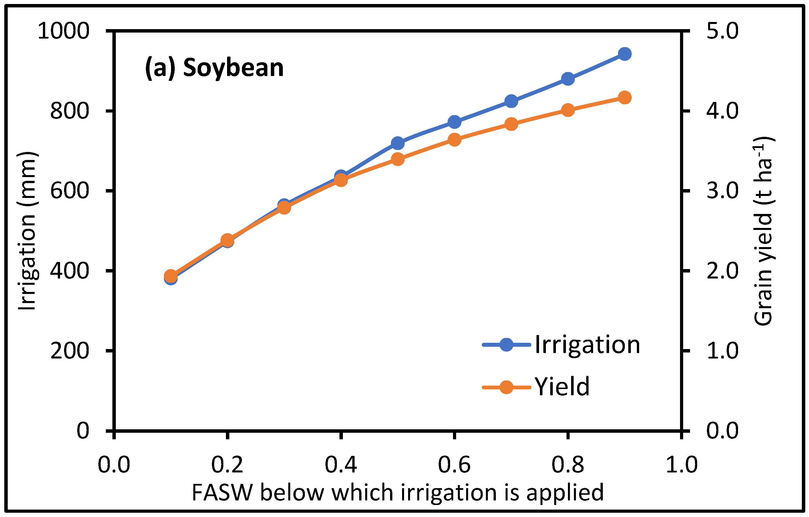
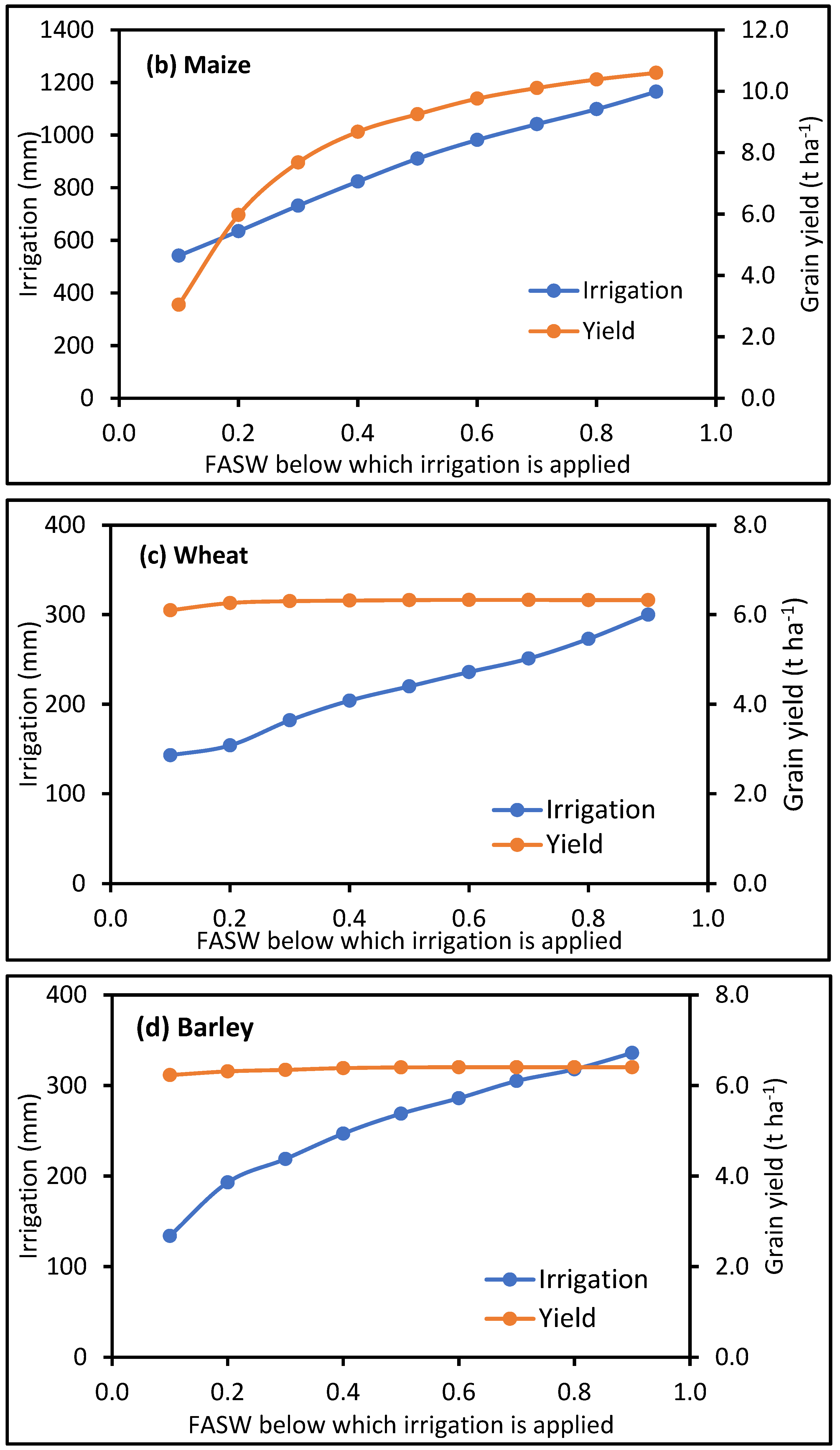
The simulated irrigation water requirement and corresponding grain yield at different soil moisture deficit levels is presented in Figure 4. The optimum irrigation, the amount of irrigation that maximises yield per unit of water applied, is: soybean, 820 mm (8.2 ML ha−1); maize, 1040 mm (10.4 ML ha−1); wheat, 250 mm (2.5 ML ha−1); barley, 310 mm (3.1 ML ha−1); fababean, 250 mm (2.5 ML ha−1); and canola, 270 mm (2.7 ML ha−1). In this study area, Gaydon et al. [3] estimated the irrigation requirement of 8 ML ha−1 for soybean and 3 ML ha−1 for barley. The relationship between grain yield, irrigation, and soil water deficit levels is different for summer (soybean, maize) and winter (canola, fababean, wheat, barley) crops. Figure 4a shows that if soybean is scheduled to be irrigated when the soil moisture is only slightly depleted (FASW 0.8), the total amount of irrigation is high. However, if irrigation is applied when the soil moisture is depleted to a level that is only 20% of the available soil water (FASW 0.2), the total amount of irrigation decreases significantly. The grain yield also follows a similar trend. However, the rate of yield increase slows when irrigation is scheduled in the high soil moisture range. Above FASW 0.5, the rate of yield increase is only 5%. However, when FASW is less than 0.5, the rate of yield increase is 20%. Figure 4b also shows that maize has a similar pattern. It has a slightly quicker increase in yield in the early part of the curve and plateaus once FASW > 0.45. The average rate of yield increase is 56% for FASW < 0.45 and it was only 3% once FASW > 0.45. This pattern is different for winter crops; there is only a slight yield increase as the amount of irrigation increases. Overall, the highest yield is obtained at the lowest soil moisture deficit level. If irrigation was to be applied only after the soil moisture was highly depleted (FASW 0.2), less irrigation would be required.
The FASW below which crop yields are affected depends on the crop species, growth stage, and environmental condition. For example, for shallow-rooted crops it is 0.25–0.40, for deep rooted-crops it is 0.50, and for deep-rooted crops with dense rooting systems it is 0.60–0.65. FAO recommends that the commonly used average FASW 0.50 should be increased by 15% when the reference evapotranspiration ETo <3 mm day−1 and decreased by 15% when ETo > 8 mm day−1 [27].
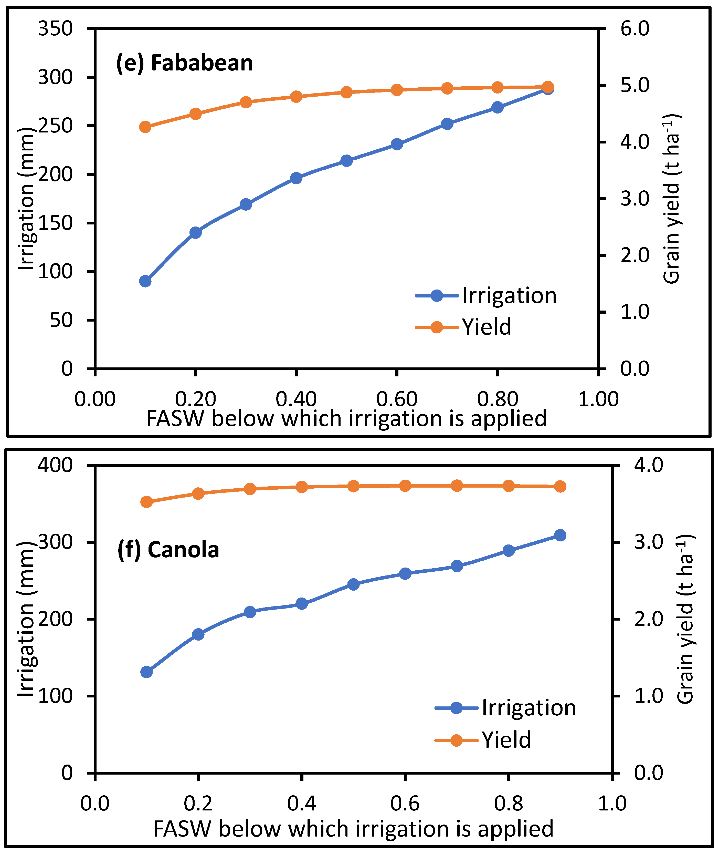
The relationship between the amount of irrigation and grain yield is presented in Figure 5. From Figure 5a (soybean), it can be seen that when irrigation was reduced from 942 to 636 mm (32%), yield dropped by 25%, and when irrigation was reduced from 564 to 381 mm (32%), yield dropped by 31%. For maize (Figure 5b), when irrigation was reduced from 1165 to 824 mm (29%), yield dropped by only 18%. However, when irrigation was reduced from 732 to 542 mm (26%), yield dropped by 60%. This shows that for soybean, the rate of crop yield loss per unit reduction in irrigation amount is the same at a higher and lower irrigation ranges. When a higher amount of irrigation is applied, some of the applied water is lost by deep percolation below the root zone [3]. There is high solar radiation and temperature during the summer period, implying no yield-limiting environmental factors. As a result, unlike winter crops, for summer crops, when a higher amount of irrigation water is applied, correspondingly a higher yield can be obtained. For soybean, the amount of irrigation that maximizes yield per unit of water is 8.2 ML ha−1 resulting in 3.8 t ha−1 yield, and for maize, it is 10.4 ML ha−1 irrigation resulting in 10.1 t ha−1 yield.
When the available soil moisture is highly depleted and the plant is unable to easily extract water, plant water stress and crop yield loss result. Different crops have different water stress tolerance [28]. The stress tolerance level also depends on the season, summer or winter. Due to low evaporative demand during the winter period, the plants are not significantly affected by the low soil moisture levels. During the summer period, however, due to high evaporative demand, the plants would not be able to withstand high soil water depletion. The total amount of irrigation is different for different soil moisture deficit levels. If irrigation was to be applied only after the soil moisture is highly depleted (long irrigation interval), the overall amount of irrigation required would be lower. However, irrigating while the soil moisture is still high results in more frequent and higher amount of irrigation. Crop water use is high when the soil moisture is high because crops can easily extract soil water. As a result, the total seasonal irrigation decreases as irrigation is applied less frequently, that is, waiting until the soil water is significantly depleted. However, this happens at the expense of crop yield.
3.2. Water Productivity of Summer and Winter Crops at Different Soil Moisture Deficit Levels
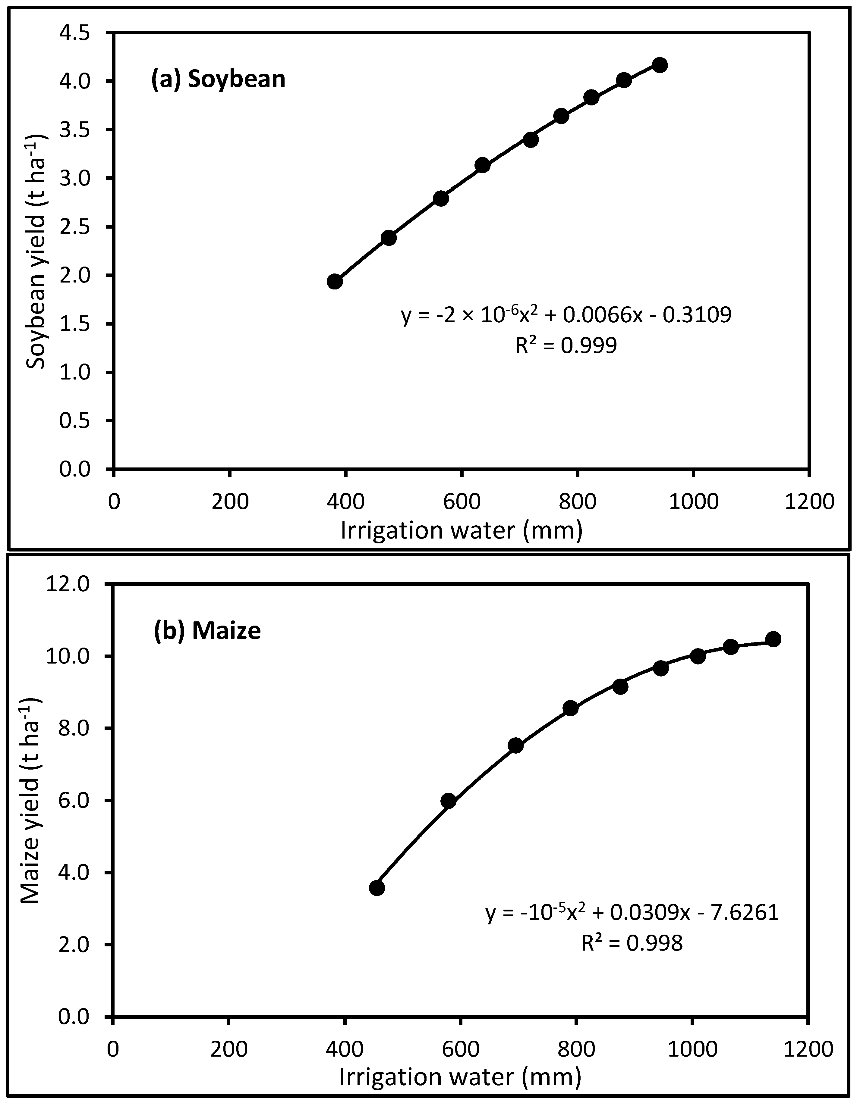
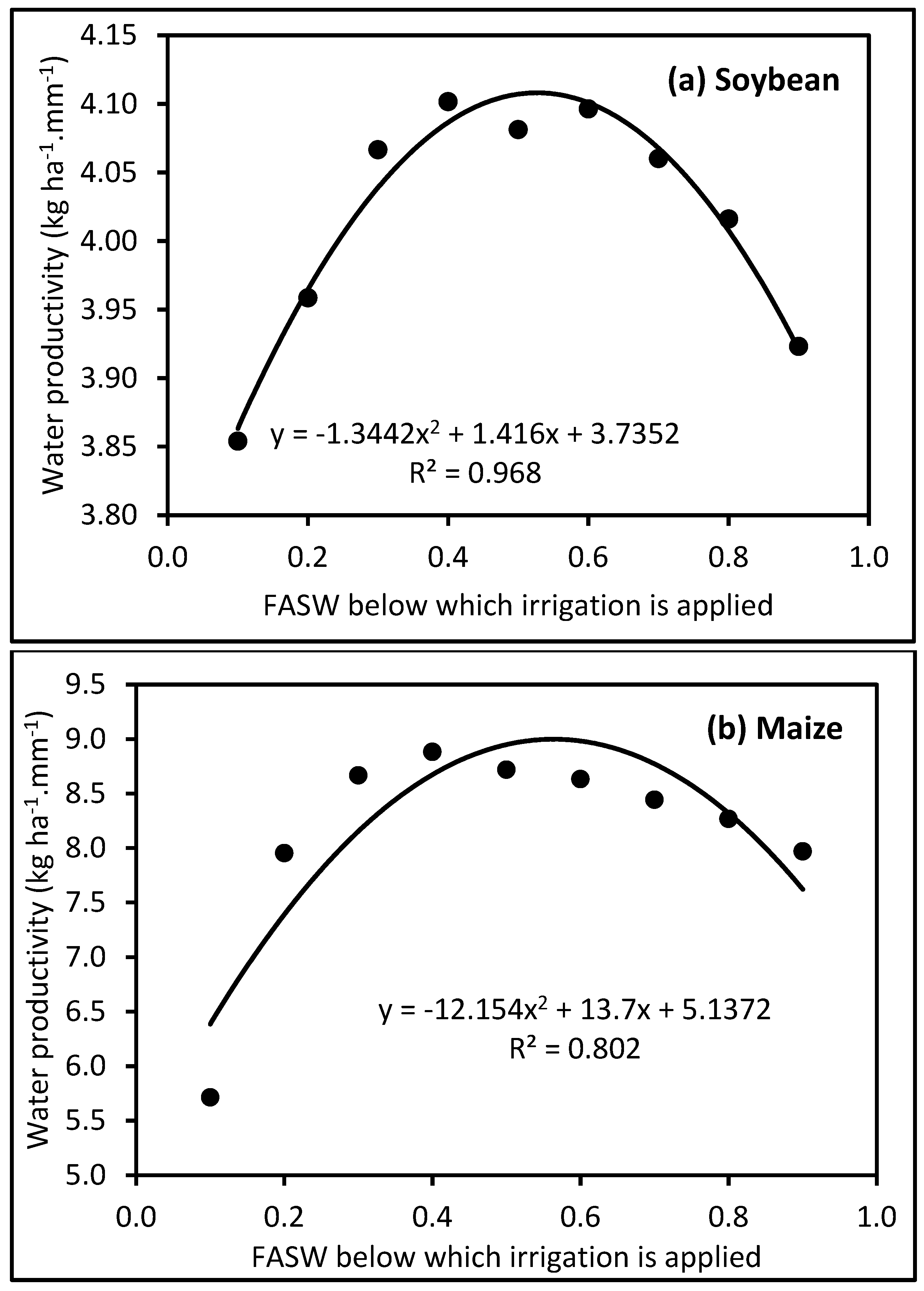
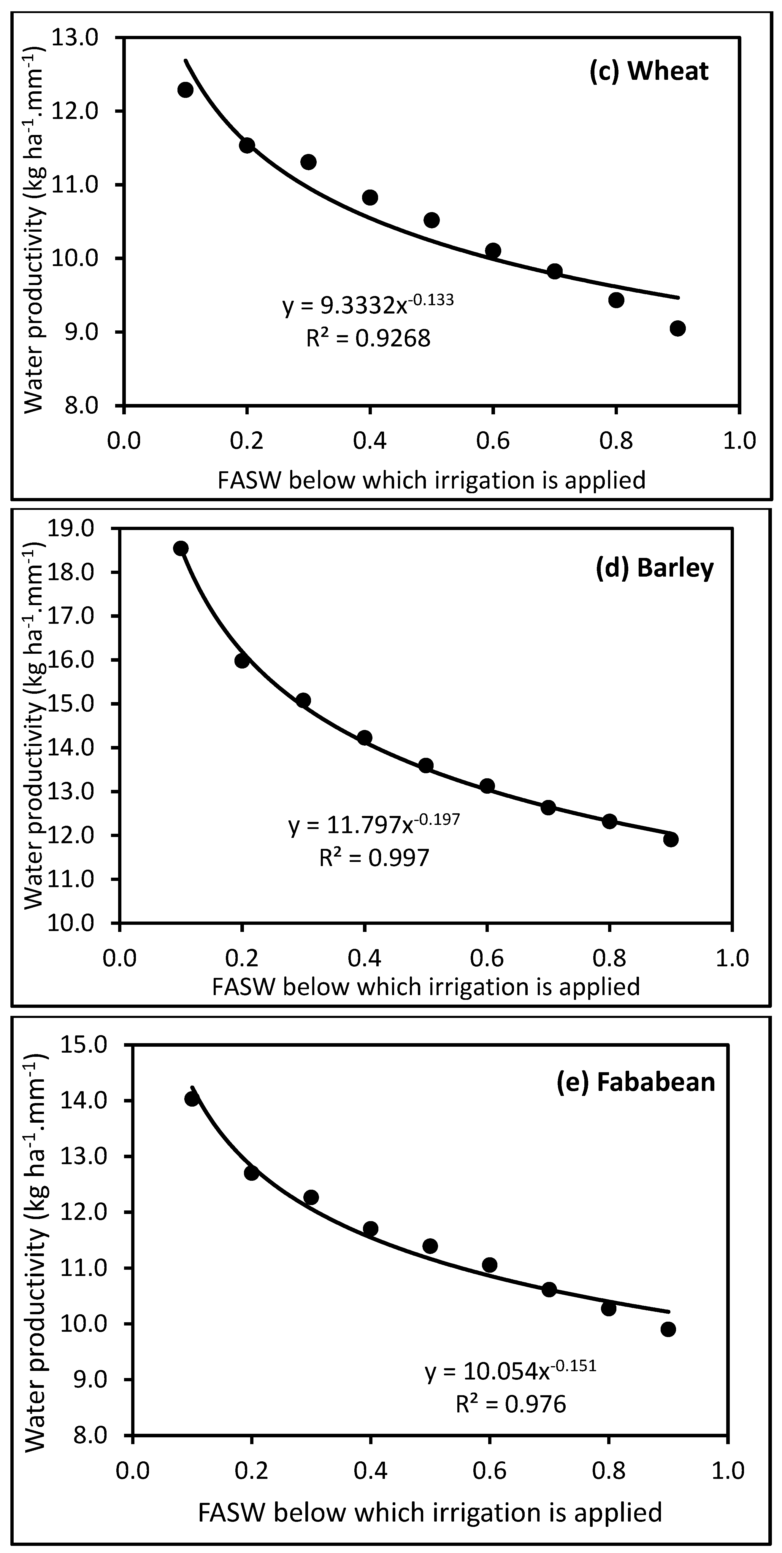
Crop water productivity was calculated as a ratio of crop yield and the total amount of water applied (rainfall plus irrigation). This was done for the water deficit levels varying from 0.1 to 0.9. The response of water productivity to different irrigation trigger soil moisture levels differs for summer and winter crops (Figure 6). The variation of water productivity with the soil water deficit levels was different for summer and winter crops. For summer crops, water productivity increases as the soil moisture level at which irrigation is applied increases. However, once it reached a maximum value at about FASW 0.5, it decreases. However, for winter crops, it starts at a higher value at FASW 0.1 and starts decreasing. This is attributed to less evapotranspiration during the winter crop growing season. Compared to the summer crops, the variation in water productivity with soil moisture depletion levels is not that high. For summer crops, if irrigation is applied only after the soil moisture drops to a low level (such as FASW 0.2), water productivity is low. It increases as the FASW increases and reaches a maximum at about FASW 0.4–0.6 before it decreases again; this is well-represented by a second-degree polynomial equation (Figure 6a,b). For winter crops, the highest water productivity is when FASW is low (e.g., FASW 0.2). From this highest point, it decreases as the FASW increases following a trend line represented by a power function (Figure 6c–f).
Summer crops have higher water requirements compared to winter crops due to high evaporative demand during the summer season. If irrigation is applied before the plant available water is depleted, the crop grows at an optimum level and yield will not be affected. However, depending on the crop type, growth stage, and crop water demand, crop yields can be affected when irrigation is applied after the soil water is depleted below a certain level called the management allowed deficit or critical soil moisture content [29]. Supplemental or deficit irrigation is practiced when irrigation is applied after the soil moisture is depleted below the critical soil moisture level. If the soil water is allowed to be depleted below the critical level before irrigation is applied, the practice is called regulated deficit irrigation [30].
3.3. Gross Margins for Different Crop Sequences
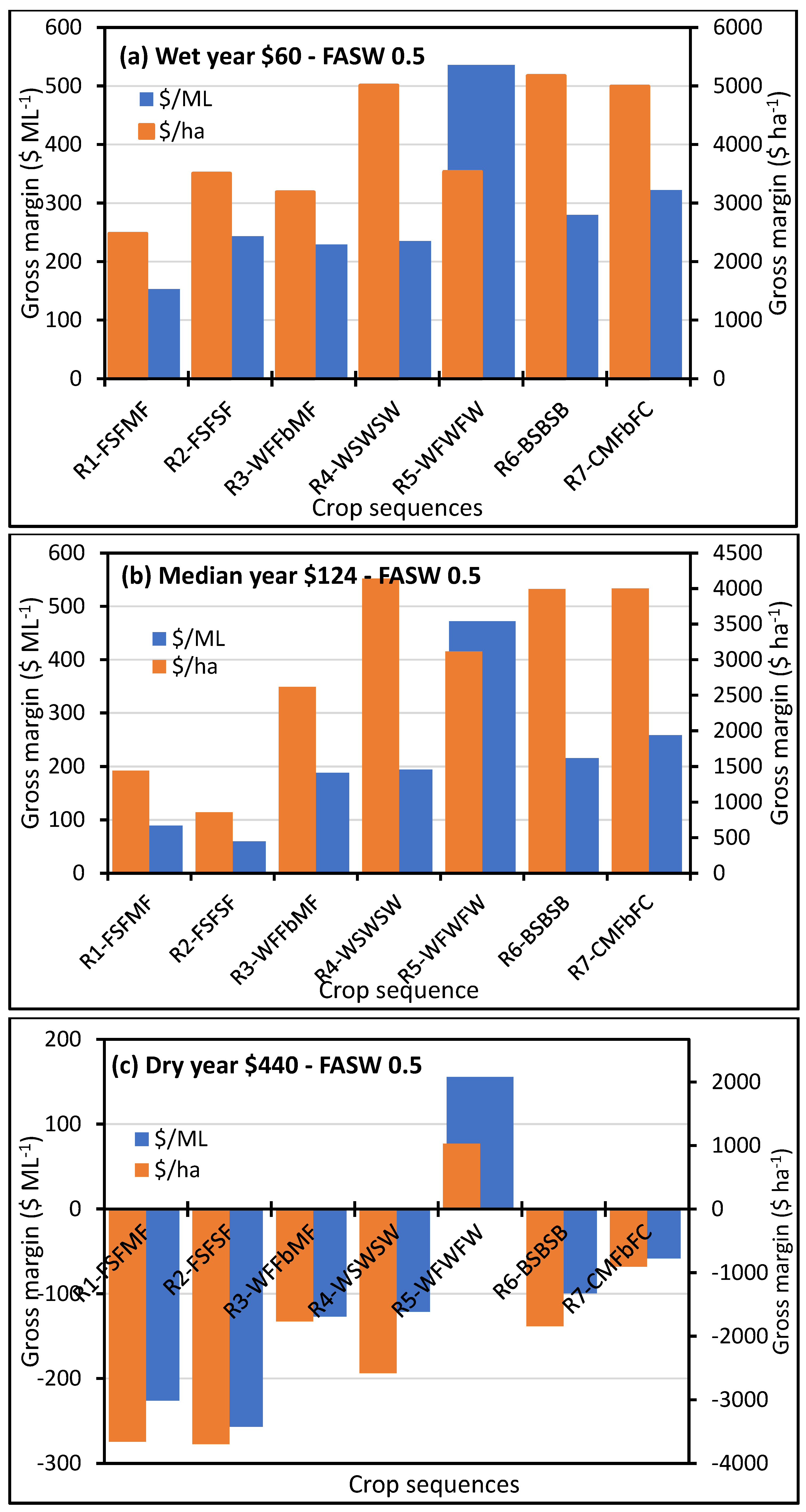
Gross margin ($ ML−1 and $ ha−1) for different water prices, soil water deficits, and crop sequences is presented in Figure 7. When irrigation water is limited, irrigation scheduling depends on the prevailing seasonal conditions and the value of water. It can be seen that when irrigation is applied at the commonly used FASW 0.5, positive gross margins were obtained under all crop sequence scenarios and the 25 percentile ($60 ML−1) and 50 percentile ($124 ML−1) water price scenarios. When water is expensive (75 percentile—$440 ML−1), all, except the continuous wheat scenario, resulted in negative gross margins. Obviously, the gross margin (both per ML and per ha) was the highest when water was cheap ($60 ML−1). When water was cheap ($60 ML−1), continuous wheat (WFWFW) resulted in the highest gross margin per unit of water used ($536 ML−1) and the lowest was for the FSFMF sequence ($153 ML−1). Per unit of cultivated land area, the two non-fallow crop sequences (WSWSW and BSBSB) resulted in the highest return, $5010 ha−1 and $5175 ha−1, respectively. When water was expensive ($440 ML−1), the biggest loss was for the soybean-only sequence (FSFSF) scenario (−$257 ML−1 and −$3696 ha−1).
Comparing the three deficit levels (FASW 0.2, FASW 0.5, FASW 0.8) under the cheap water scenario ($60 ML−1), the highest gross margin per ML was obtained for the WFWFW crop sequence. The gross margin for the three soil water deficit levels FASW 0.2, FASW 0.5, and FASW 0.8 was $781 ML−1, $536 ML−1, and $420 ML−1, respectively. For all of the three water deficit scenarios, the highest per unit area gross margin would be obtained for crop sequences where there is neither summer nor winter fallow (WSWSW and BSBSB). The highest per unit area gross margin was obtained for the FASW 0.8. For example, considering the WSWSW scenario, the gross margin per cultivated land area was 5881 $ ha−1, 5010 $ ha−1, and 4542 $ ha−1, for the FASW 0.8, FASW 0.5, and FASW 0.2 scenarios, respectively.
When water is expensive ($440 ML−1), under all three soil moisture deficit levels, only the WFWFW crop sequence resulted in a positive gross margin. For this crop sequence, under the expensive water scenario, the highest gross margin (as $ ML−1) was when FASW was 0.8. The gross margin as $ ML−1 for the three soil moisture deficit scenarios FASW 0.2, FASW 0.5, and FASW 0.8 was 429 $ ML−1, 156 $ ML−1, and 41 $ ML−1, respectively. Per unit of cultivated land area it also followed a similar pattern, 1930 $ ha−1, 1028 $ ha−1, and 335 $ ha−1 for FASW 0.2, FASW 0.5, and FASW 0.8, respectively. The biggest loss in gross margin as $ ML−1 was for the only-soybean scenario FSFSF. The gross margin losses were −$272 ML−1, −$257 ML−1, and −$253 ML−1, for FASW 0.2, FASW 0.5, and FASW 0.8, respectively. The biggest gross margin loss per ha was also for the soybean-only scenario FSFSF. The gross margin losses were −4457 $ ha−1, −3696 $ ha−1, and −2561 $ ha−1 for FASW 0.8, FASW 0.5, and FASW 0.2, respectively.
When water is plentiful and cheap and land is not limited, full irrigation of winter and summer crops that results in high return per unit of water and land area can be practiced. However, when water is limited, partial/deficit irrigation results in better return in $ per ML. A high gross margin per unit area ($ ha−1) is obtained when both summer and winter crops are sown (i.e., no fallow). Crop intensification can minimize the expansion of agricultural land, although its viability depends on attainable crop yield [2].
3.4. Gross Margin under Different Water Price and Soil Water Deficit Scenarios
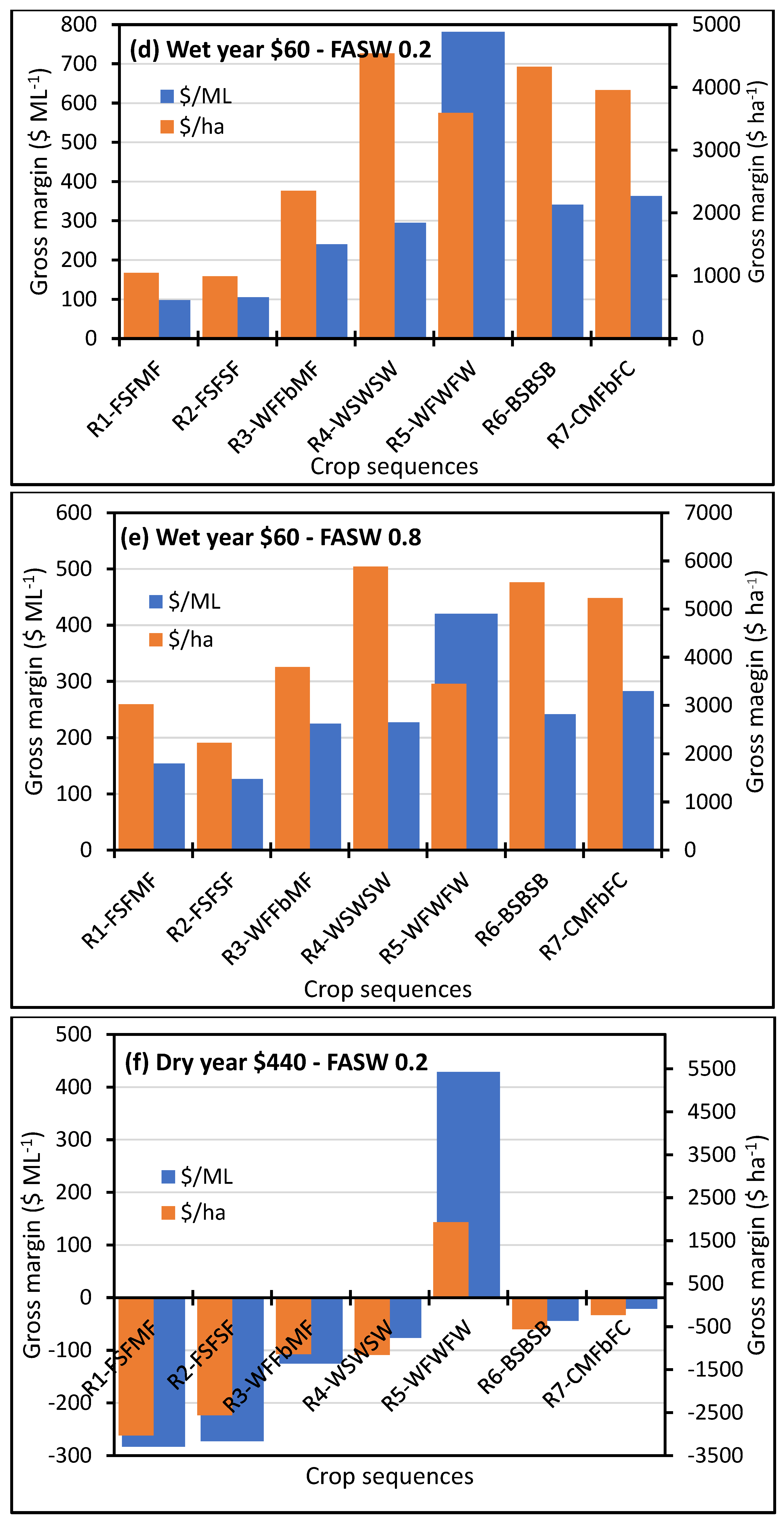
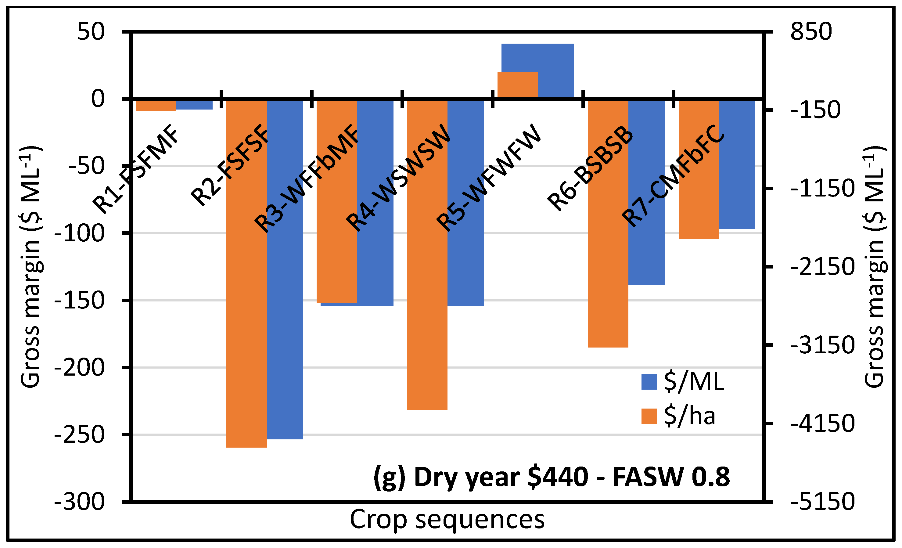
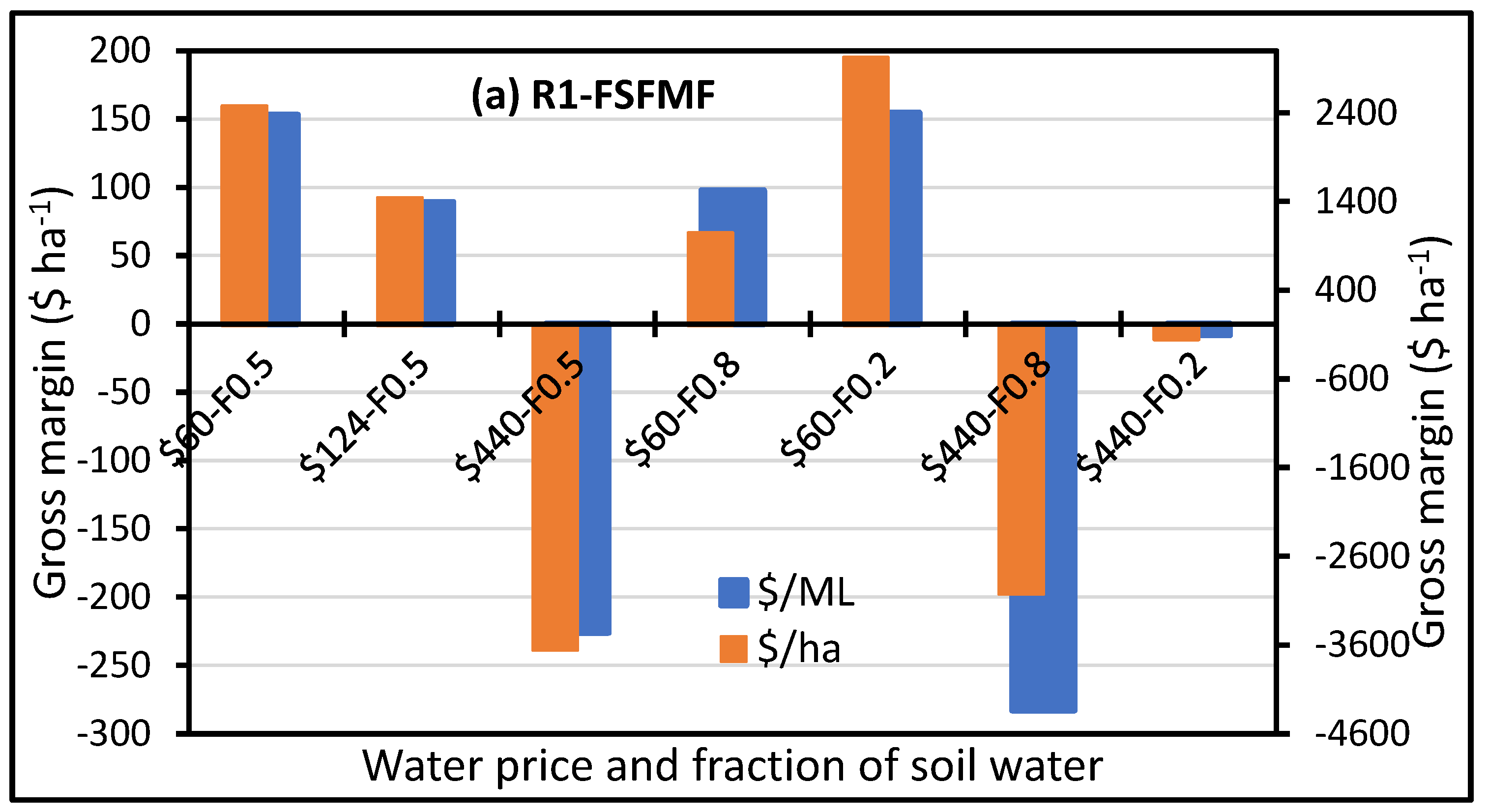
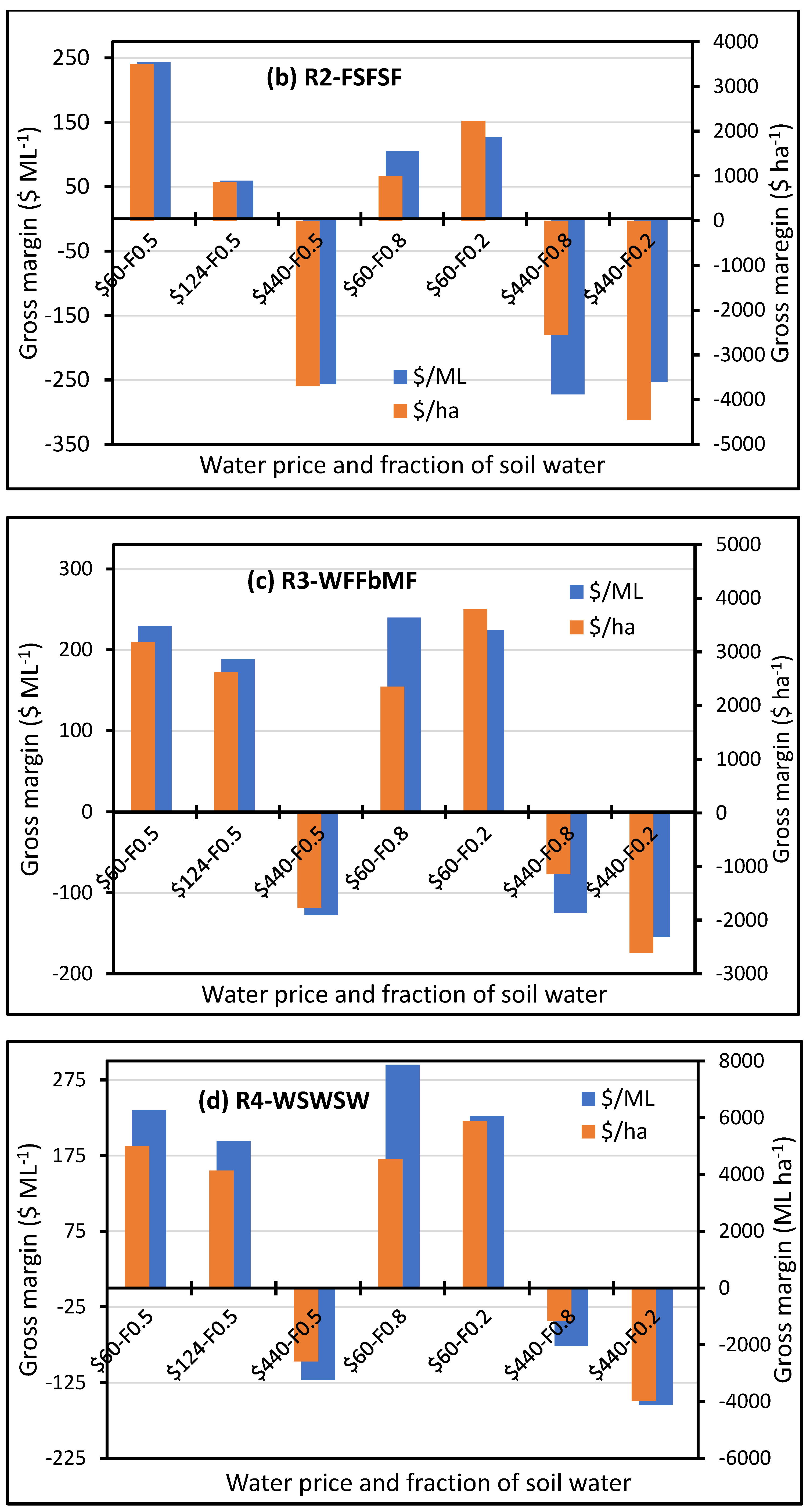
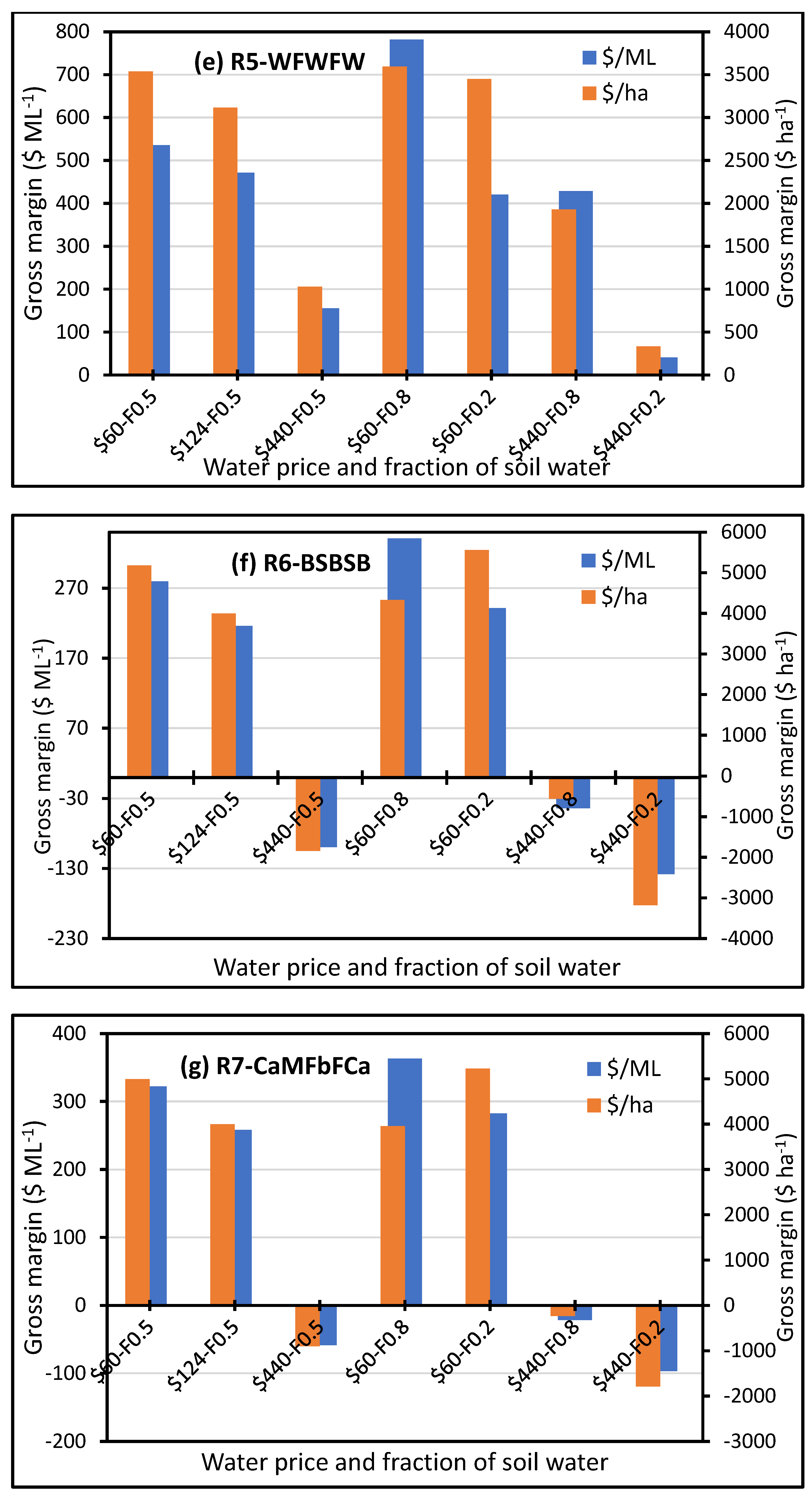
One of the factors determining the gross margin of an irrigated farm is the price of water, which varies with the amount of rainfall received by the catchments and runoff into reservoirs. There is significant year to year rainfall variability in Australia. Water trade was instituted in Australia to move water from where it has a lower value to where it can be used at its highest value (e.g., for permanent horticulture). The Australian water market is highly complex and occurs across catchments and state boundaries. For this study, 15 years’ water price data in the Murrumbidgee catchment were used. Accordingly, the 25 percentile water price ($) was $60 ML−1, the median water price was $124 ML−1, and the 75 percentile water price was $440 ML−1. The gross margin was determined for the three water prices and different irrigation scheduling criteria. Irrigation could be applied at different soil moisture deficit levels between field capacity (drained upper limit) and permanent wilting point (drained lower limit). From Figure 8a it can be seen that having two summer crops (soybean and maize) with winter fallows in between has positive gross margins ($ ML−1 and $ ha−1) for 25 percentile and median water prices with the gross margin of the $60 water price being higher than that of the median price $124. When water is cheap, all crop sequence scenarios resulted in positive gross margins (Figure 8a–g). At a higher water price of $440 ML−1, the gross margins were negative. At an intermediate water price ($124 ML−1), all crop sequences resulted in positive gross margins for an FASW of 0.5. The highest gross margin ($ ML−1 and $ ha−1) was for the winter crop-only sequence R5-WFWFW, while the lowest was for the summer crop-only sequence R2-FSFSF. A water price of $60 ML−1 and FASW 0.8 resulted in the highest yield and profit when winter crops are gown. However, for a summer crop-only sequence or when there is at least one season summer crop, partial irrigations (FASW 0.2 and 0.5) resulted in better gross margins. In seasons with low water allocation and when water is expensive, maximizing crop yields does not necessarily lead to the highest whole-farm gross margins.
When seasonal allocation is low and water is expensive, farmers need to concentrate on fully irrigated winter cropping. This can be seen from Figure 8, where at 440 $ ML−1 all of the crop sequence scenarios resulted in negative gross margins both per unit of water and per unit of land area. The only scenario that resulted in a positive gross margin was R5-WFWFW (Figure 4e), where the gross margin at all three soil moisture deficit levels was positive. The gross margin was highest for the full irrigation (FASW 0.8) and lowest for the deficit irrigation scenario (FASW 0.2). The 50% deficit (FASW 0.5) resulted in the intermediate gross margin.
Historically, irrigation allocation was close to 100%. However, in recent years the allocation has been much lower. This requires maximising crop yield and profit per unit of water. For winter crops, the greatest yield return per unit of water is when about 200–300 mm (2–3 ML ha−1) of irrigation water is applied. Above this amount, the rate of return of yield for each unit of irrigation water applied decreases (diminishing rate of return). The relationship between crop production and transpiration is linear [31]; hence this decreased slope shows that there are other yield-limiting factors. For winter crops, solar radiation and temperature are the liming factors. Even if a higher amount of irrigation water is applied, the crops do not grow in proportion to the amount of water applied. However, in this study, for summer crops the yield continued to increase as the amount of irrigation was increased.
4. Conclusions
This study evaluated different crop sequence, irrigation scheduling and water price scenarios to improve the whole-farm gross margin. APSIM, the agricultural system model used in this study, is a vital tool in prioritizing the use of limited resources such as water and land. The analyses demonstrated that when water supply is not limited and full irrigation is practiced, irrigation needs to be triggered with only small soil water deficits, leading to smaller but frequent irrigations, generally resulting in a higher total irrigation. When full irrigation is not possible due to limited water supply, irrigation should be applied only after the soil water is highly depleted, leading to larger but fewer irrigation events and, generally, a lower amount of total irrigation. These strategies can be used to maximise long-term profitability.
Summer and winter crops show different relationships between water productivity and soil water deficit levels. Summer crops have a parabolic relationship with water productivity, increasing, reaching a maximum, and then decreasing as the amount of irrigation increases. Winter crops, however, have the highest water productivity at the lowest irrigation level.
In the current environment, and more so in the future water-limited environment, supplemental irrigation of winter crops will have more whole farm return compared to fully irrigated intensive winter–summer cropping systems. When water is limited, it would be better to practice supplemental irrigation of a winter crop rather than full irrigation of a summer crop. In hot and dry environments such as the Riverina region, deficit irrigation of summer crops is not a viable option due to high evaporative demand. However, this needs to be decided based on the relative price of summer and winter crops as well. In order to maximise long-term average returns, farm management strategies that vary on a season-by-season basis, based on resource availability, cost, and commodity prices, are required.
The interaction between relative prices of summer and winter crops and different irrigation water allocations was not considered. The gross margin comparison as influenced by the fluctuation in commodity prices needs to be investigated in any future study. Farm return was evaluated only from the water and land value perspective; for example, addition of nitrogen by legumes was not considered.
Author Contributions
Conceptualization, methodology, software: K.Z.; investigation, visualization, writing: K.Z. and J.M. All authors have read and agreed to the published version of the manuscript.
Funding
This research received no external funding.
Institutional Review Board Statement
Not applicable.
Informed Consent Statement
Not applicable.
Acknowledgments
Charles Sturt University for paying the publication processing fee.
Conflicts of Interest
There is no conflict of interest to declare.
References
- Ray, D.K.; Foley, J.A. Increasing global crop harvest frequency: Recent trends and future directions. Environ. Res. Lett. 2013, 8, 44041. [Google Scholar] [CrossRef]
- Waha, K.; Dietrich, J.P.; Portmann, F.T.; Siebert, S.; Thornton, P.K.; Bondeau, A.; Herrero, M. Multiple cropping systems of the world and the potential for increasing cropping intensity. Glob. Environ. Chang. 2020, 64, 102131. [Google Scholar] [CrossRef] [PubMed]
- Gaydon, D.; Meinke, H.; Rodriguez, D. The best farm-level irrigation strategy changes seasonally with fluctuating water availability. Agric. Water Manag. 2012, 103, 33–42. [Google Scholar] [CrossRef]
- Fereres, E.; Soriano, M.A. Deficit irrigation for reducing agricultural water use. J. Exp. Bot. 2007, 58, 147–159. [Google Scholar] [CrossRef] [PubMed] [Green Version]
- Howell, T.A. Enhancing Water Use Efficiency in Irrigated Agriculture. Agron. J. 2001, 93, 281–289. [Google Scholar] [CrossRef] [Green Version]
- Lorite, I.; Mateos, L.; Orgaz, F.; Fereres, E. Assessing deficit irrigation strategies at the level of an irrigation district. Agric. Water Manag. 2007, 91, 51–60. [Google Scholar] [CrossRef] [Green Version]
- Holzworth, D.P.; Huth, N.I.; Devoil, P.G.; Zurcher, E.J.; Herrmann, N.I.; McLean, G.; Chenu, K.; van Oosterom, E.J.; Snow, V.; Murphy, C.; et al. APSIM—Evolution towards a new generation of agricultural systems simulation. Environ. Model. Softw. 2014, 62, 327–350. [Google Scholar] [CrossRef]
- Zhang, X.; Wang, Y.; Sun, H.; Chen, S.; Shao, L. Optimizing the yield of winter wheat by regulating water consumption during vegetative and reproductive stages under limited water supply. Irrig. Sci. 2013, 31, 1103–1112. [Google Scholar] [CrossRef]
- Serafin, L.; Hertel, K.; Moore, N. Summer Crop Management Guide; NSW Department of Primary Industries: Sydney, NSW, Australia, 2019. Available online: https://www.dpi.nsw.gov.au/__data/assets/pdf_file/0011/1187750/SCMG-web-FINAL-5Nov.pdf (accessed on 18 October 2021).
- Dodig, D.; Kandić, V.; Zorić, M.; Nikolić-Đorić, E.; Nikolić, A.; Mutavdžić, B.; Perović, D.; Šurlan-Momirović, G. Comparative kernel growth and yield components of two- and six-row barley (Hordeum vulgare) under terminal drought simulated by defoliation. Crop Pasture Sci. 2018, 69, 1215–1224. [Google Scholar] [CrossRef]
- Felton, W.L.; Marcellos, H.; Alston, C.; Martin, R.J.; Backhouse, D.; Burgess, L.W.; Herridge, D.F. Chickpea in wheat-based cropping systems of northern New South Wales. II. Influence on biomass, grain yield, and crown rot in the following crop. Aust. J. Agric. Res. 1998, 49, 401–407. [Google Scholar] [CrossRef]
- Matthews, P.; McCaffery, D.; Jenkins, L. Winter Crop Variety Sowing Guide 2017; NSW Department of Primary Industries: Sydney, NSW, Australia, 2017. Available online: https://www.dpi.nsw.gov.au/__data/assets/pdf_file/0017/1302173/nsw-dpi-wcvsg-2021-web.pdf (accessed on 24 September 2021).
- Kirkegaard, J.A.; Hunt, J.R. Increasing productivity by matching farming system management and genotype in water-limited environments. J. Exp. Bot. 2010, 61, 4129–4143. [Google Scholar] [CrossRef] [PubMed] [Green Version]
- Sissons, M.; Ovenden, B.; Adorada, D.; Milgate, A. Durum wheat quality in high-input irrigation systems in south-eastern Australia. Crop Pasture Sci. 2014, 65, 411–422. [Google Scholar] [CrossRef]
- Jeffrey, S.J.; Carter, J.O.; Moodie, K.B.; Beswick, A.R. Using spatial interpolation to construct a comprehensive archive of Australian climate data. Environ. Model. Softw. 2001, 16, 309–330. [Google Scholar] [CrossRef]
- ApSoil. A Database of Soil Characteristics. 2013. Available online: http://www.apsim.info/Products/APSoil.aspx (accessed on 24 August 2021).
- Lilley, J.M.; Bell, L.W.; Kirkegaard, J. Optimising grain yield and grazing potential of crops across Australia’s high-rainfall zone: A simulation analysis. 2. Canola. Crop Pasture Sci. 2015, 66, 349–364. [Google Scholar] [CrossRef]
- Zeleke, K.; Nendel, C. Analysis of options for increasing wheat (Triticum aestivum L.) yield in south-eastern Australia: The role of irrigation, cultivar choice and time of sowing. Agric. Water Manag. 2016, 166, 139–148. [Google Scholar] [CrossRef]
- Archontoulis, S.V.; Miguez, F.E.; Moore, K.J. A methodology and an optimization tool to calibrate phenology of short-day species included in the APSIM PLANT model: Application to soybean. Environ. Model. Softw. 2014, 62, 465–477. [Google Scholar] [CrossRef]
- Turpin, J.E.; Robertson, M.J.; Haire, C.; Bellotti, W.D.; Moore, A.D.; Rose, I. Simulating fababean development, growth, and yield in Australia. Aust. J. Agric. Res. 2003, 54, 39–52. [Google Scholar] [CrossRef]
- Zeleke, K.; Nendel, C. Growth and yield response of faba bean to soil moisture regimes and sowing dates: Field experiment and modelling study. Agric. Water Manag. 2019, 213, 1063–1077. [Google Scholar] [CrossRef]
- Peake, A.S.; Robertson, M.J.; Bidstrup, R.J. Optimising maize plant population and irrigation strategies on the Darling Downs using the APSIM crop simulation model. Aust. J. Exp. Agric. 2008, 48, 313–325. [Google Scholar] [CrossRef]
- Liu, K.; Harrison, M.T.; Hunt, J.; Angessa, T.T.; Meinke, H.; Li, C.; Tian, X.; Zhou, M. Identifying optimal sowing and flowering periods for barley in Australia: A modelling approach. Agric. For. Meteorol. 2010, 282–283, 107871. [Google Scholar] [CrossRef]
- Robertson, M.J.; Kirkegaard, J.A. Water-use efficiency of dryland canola in an equi-seasonal rainfall environment. Aust. J. Agric. Res. 2005, 56, 1373–1386. [Google Scholar] [CrossRef]
- Zeleke, K.; Luckett, D.; Cowley, R. The influence of soil water conditions on canola yields and production in Southern Australia. Agric. Water Manag. 2014, 144, 20–32. [Google Scholar] [CrossRef]
- Napier, T.; Gaynor, L.; Johnston, D.; Morris, G.; Rollin, M. Crop Sequencing for Irrigated Double Cropping—Murrumbidgee Valley Site. GRDC Update. 2016, pp. 95–99. Available online: https://grdc.com.au/resources-and-publications/grdc-update-papers/tab-content/grdc-update-papers/2016/07/crop-sequencing-for-irrigated-double-cropping-murrumbidgee-valley-site (accessed on 8 September 2021).
- Allen, R.; Pereira, L.S.; Raes, D.; Smith, M. Crop Evapotranspiration: Guidelines for Computing Crop Water Requirements; FAO Irrigation and Drainage Paper No 56; FAO: Rome, Italy, 1998; 300p. [Google Scholar]
- Osakabe, Y.; Osakabe, K.; Shinozaki, K.; Tran, L.-S.P. Response of plants to water stress. Front. Plant Sci. 2014, 5, 86. [Google Scholar] [CrossRef] [PubMed] [Green Version]
- Soothar, R.K.; Singha, A.; Soomro, S.A.; Chachar, A.-U.; Kalhoro, F.; Rahaman, A. Effect of different soil moisture regimes on plant growth and water use efficiency of Sunflower: Experimental study and modeling. Bull. Natl. Res. Cent. 2021, 45, 121. [Google Scholar] [CrossRef]
- Chai, Q.; Gan, Y.; Zhao, C.; Xu, H.-L.; Waskom, R.M.; Niu, Y.; Siddique, K.H. Regulated deficit irrigation for crop production under drought stress. A review. Agron. Sustain. Dev. 2015, 36, 3. [Google Scholar] [CrossRef] [Green Version]
- Perry, C.; Steduto, P.; Allen, R.G.; Burt, C.M. Increasing productivity in irrigated agriculture: Agronomic constraints and hydrological realities. Agric. Water Manag. 2009, 96, 1517–1524. [Google Scholar] [CrossRef] [Green Version]
Figure 1.
Historical annual percentage allocation of irrigation water entitlement in the Murrumbidgee Irrigation Area, Riverina, NSW (data from https://www.industry.nsw.gov.au/water/allocations-availability/water-accounting/historical-available-water-determination-data, accessed on 20 November 2021).

Figure 2.
Mean monthly rainfall, temperature and evapotranspiration at Leeton station, Riverina region, NSW Australia (1989–2018).
Figure 2.
Mean monthly rainfall, temperature and evapotranspiration at Leeton station, Riverina region, NSW Australia (1989–2018).

Figure 3.
Water price as a function of seasonal water allocation in the Murrumbidgee valley of NSW, Australia.
Figure 3.
Water price as a function of seasonal water allocation in the Murrumbidgee valley of NSW, Australia.

Figure 4.
The amount of irrigation and corresponding grain yield of summer and winter crops for different soil water deficit levels in the Riverina region, NSW, Australia.
Figure 4.
The amount of irrigation and corresponding grain yield of summer and winter crops for different soil water deficit levels in the Riverina region, NSW, Australia.


Figure 5.
Simulated water production function of soybean and maize and fitted polynomial function in the Riverina region of NSW, Australia.
Figure 5.
Simulated water production function of soybean and maize and fitted polynomial function in the Riverina region of NSW, Australia.

Figure 6.
Water productivity of summer and winter crops at different soil water deficit levels in the Riverina region of NSW, Australia.
Figure 6.
Water productivity of summer and winter crops at different soil water deficit levels in the Riverina region of NSW, Australia.


Figure 7.
Total gross margin per unit of water and per cultivated land for different water prices ($) and available soil water fractions (FASW) as affected by crop sequences. Wet, medium, and dry refer to years with above average, average, and below average rainfall, respectively.
Figure 7.
Total gross margin per unit of water and per cultivated land for different water prices ($) and available soil water fractions (FASW) as affected by crop sequences. Wet, medium, and dry refer to years with above average, average, and below average rainfall, respectively.


Figure 8.
Total gross margin per unit of water and per unit cultivated land for different water prices ($) and available soil water fractions (F).
Figure 8.
Total gross margin per unit of water and per unit cultivated land for different water prices ($) and available soil water fractions (F).


Table 1.
Hydrologic properties of the Brown Chromosol soil in Murrumbidgee Irrigation Area, NSW Australia (http://www.apsim.info) (accessed on 4 August 2021).
Table 1.
Hydrologic properties of the Brown Chromosol soil in Murrumbidgee Irrigation Area, NSW Australia (http://www.apsim.info) (accessed on 4 August 2021).
| Soil Depth (cm) | Bulk Density (g cm−3) | Wilting Point (LL15) * (cm3 cm−3) | Field Capacity (DUL) + (cm3 cm−3) | Saturation Moisture Content (cm3 cm−3) | Plant Available Water Capacity, PAWC (mm) |
|---|---|---|---|---|---|
| 0–15 | 1.47 | 0.101 | 0.265 | 0.414 | 24.6 |
| 15–30 | 1.44 | 0.247 | 0.375 | 0.427 | 19.2 |
| 30–60 | 1.43 | 0.244 | 0.380 | 0.430 | 40.8 |
| 60–90 | 1.50 | 0.244 | 0.354 | 0.404 | 32.7 |
| 90–120 | 1.58 | 0.228 | 0.325 | 0.375 | 29.1 |
| 120–150 | 1.59 | 0.224 | 0.319 | 0.366 | 26.7 |
| 150–160 | 1.49 | 0.224 | 0.324 | 0.408 | 17.7 |
* LL15 is the soil water content at 15 bar pressure, which is the lower limit of the plant available water. + DUL (drainable upper limit) is the soil water content at field capacity.
Table 2.
Winter–summer crop sequence scenarios used in the simulation.
| Rotation 1—R1 | F-S-F-M-F | Fallow–Soybean–Fallow–Maize–Fallow |
| Rotation 2—R2 | F-S-F-S-F | Fallow–Soybean–Fallow–Soybean–Fallow |
| Rotation 3—R3 | W-F-Fb-M-F | Wheat–Fallow–Fababean–Maize–Fallow |
| Rotation 4—R4 | W-S-W-S-W | Wheat–Soybean–Wheat–Soybean–Wheat |
| Rotation 5—R5 | W-F-W-F-W | Wheat–Fallow–Wheat–Fallow–Wheat |
| Rotation 6—R6 | B-S-B-S-B | Barley–Soybean–Barley–Soybean–Barley |
| Rotation 7—R7 | C-M-Fb-F-C | Canola–Maize–Fababean–Fallow–Canola |
Publisher’s Note: MDPI stays neutral with regard to jurisdictional claims in published maps and institutional affiliations. |
© 2022 by the authors. Licensee MDPI, Basel, Switzerland. This article is an open access article distributed under the terms and conditions of the Creative Commons Attribution (CC BY) license (https://creativecommons.org/licenses/by/4.0/).
Share and Cite
MDPI and ACS Style
Zeleke, K.; McCormick, J. Crop Sequencing to Improve Productivity and Profitability in Irrigated Double Cropping Using Agricultural System Simulation Modelling. Agronomy 2022, 12, 1229. https://doi.org/10.3390/agronomy12051229
AMA Style
Zeleke K, McCormick J. Crop Sequencing to Improve Productivity and Profitability in Irrigated Double Cropping Using Agricultural System Simulation Modelling. Agronomy. 2022; 12(5):1229. https://doi.org/10.3390/agronomy12051229
Chicago/Turabian StyleZeleke, Ketema, and Jeff McCormick. 2022. "Crop Sequencing to Improve Productivity and Profitability in Irrigated Double Cropping Using Agricultural System Simulation Modelling" Agronomy 12, no. 5: 1229. https://doi.org/10.3390/agronomy12051229
Note that from the first issue of 2016, this journal uses article numbers instead of page numbers. See further details here.