
Evaluation of SEBS, METRIC-EEFlux, and QWaterModel Actual Evapotranspiration for a Mediterranean Cropping System in Southern Italy

 , , , , and
Abstract
:1. Introduction
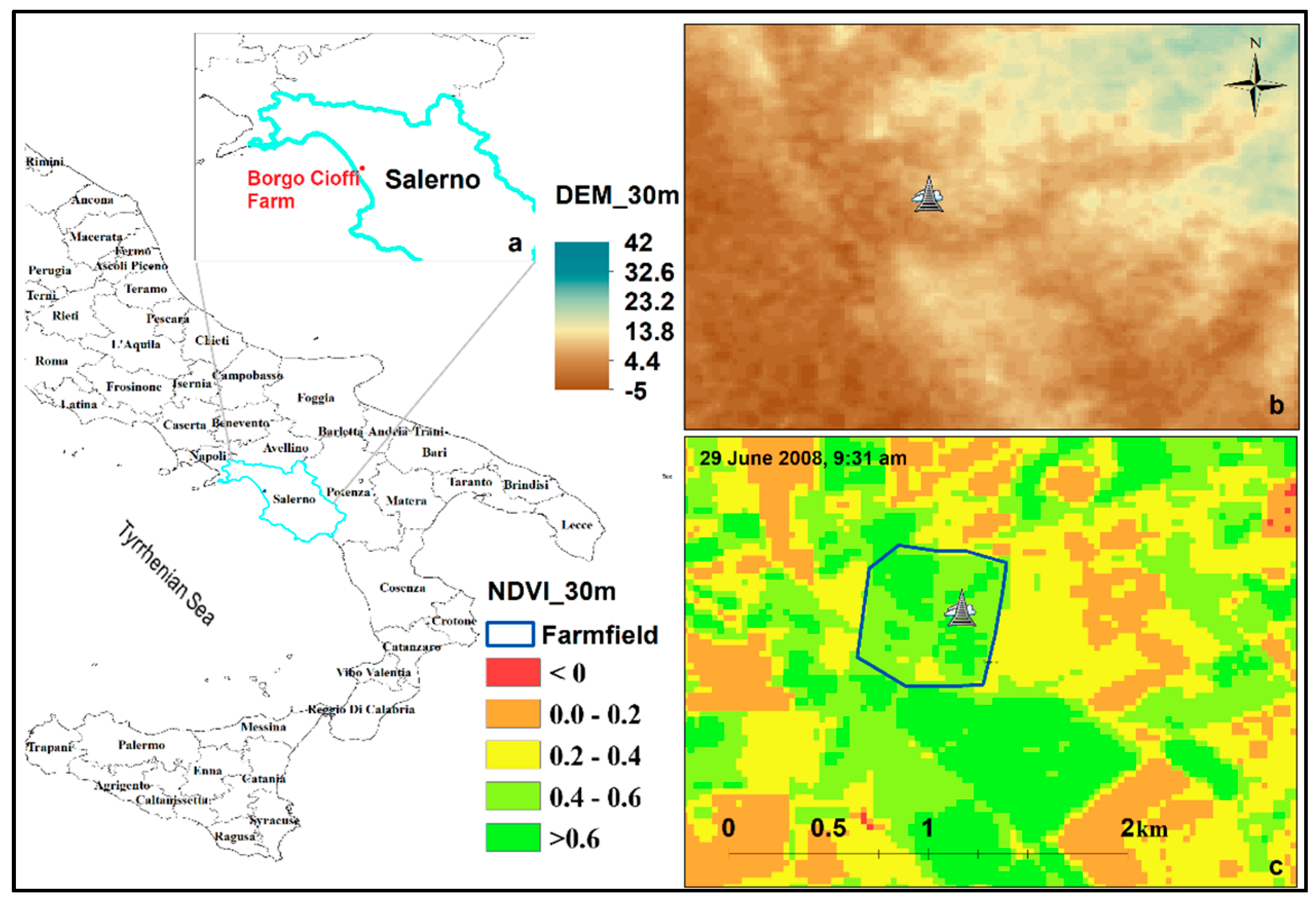
2. Site Features
3. Materials and Methods
3.1. Ground-Based Actual Evapotranspiration (ETa) Estimates
3.2. Ground-Based Reference ET (ETO_FAO56)
3.3. Remote Sensing Data and Retrievals
- ee. Algorithms.Landsat. simpleCloudScore
- ee. Algorithms.Landsat. calibratedRadiance
- ee. Algorithms.Landsat.TOA
3.4. Crop Field Related Measurements
3.5. Energy Balance Models
3.5.1. Mapping Evapotranspiration at High Resolution with Internalized Calibration- (METRIC)-EEFlux
3.5.2. Surface Energy Balance System (SEBS)
3.5.3. QWaterModel
3.6. Validation of Model-Based ETa
4. Results and Discussion
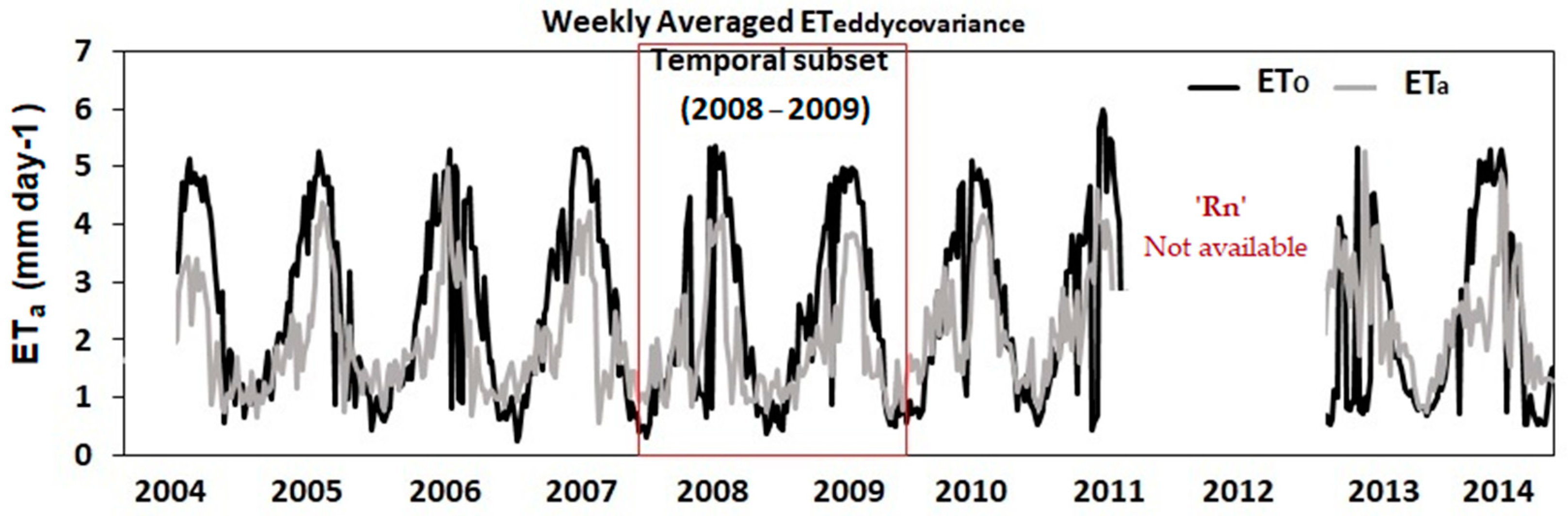
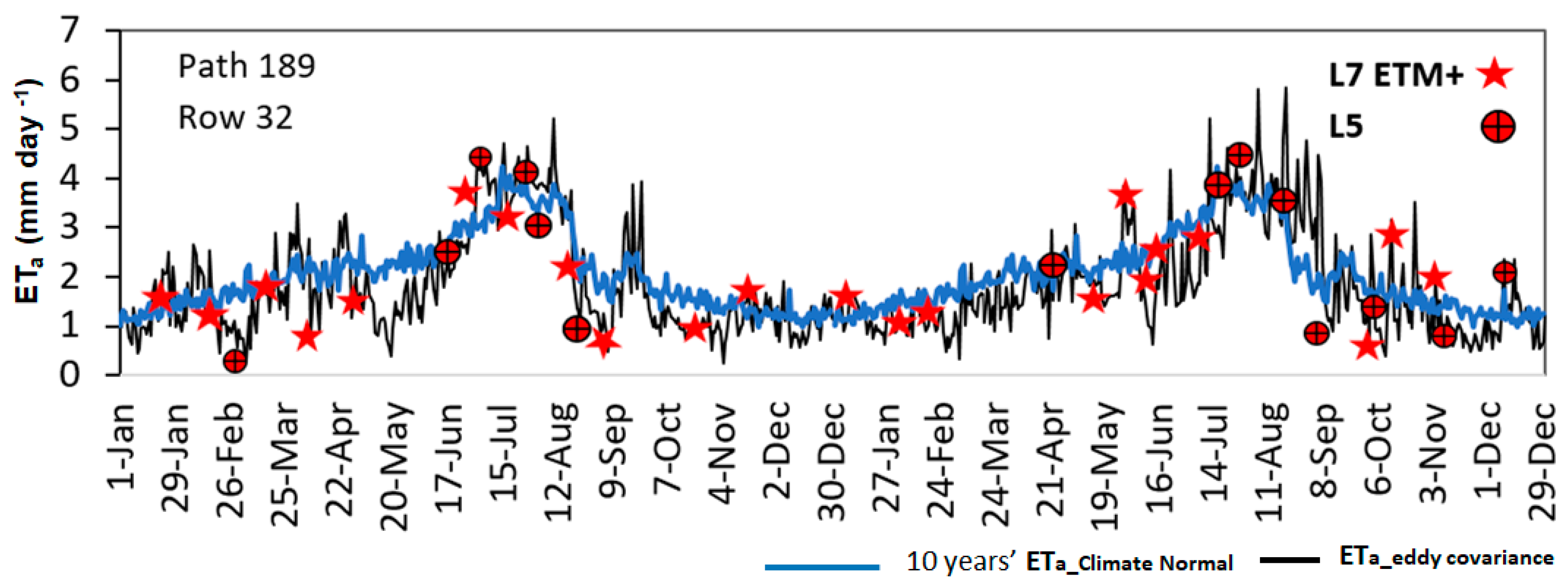
4.1. Averaged Ground Based Evapotranspiration (ET) Trend and Temporal Selection
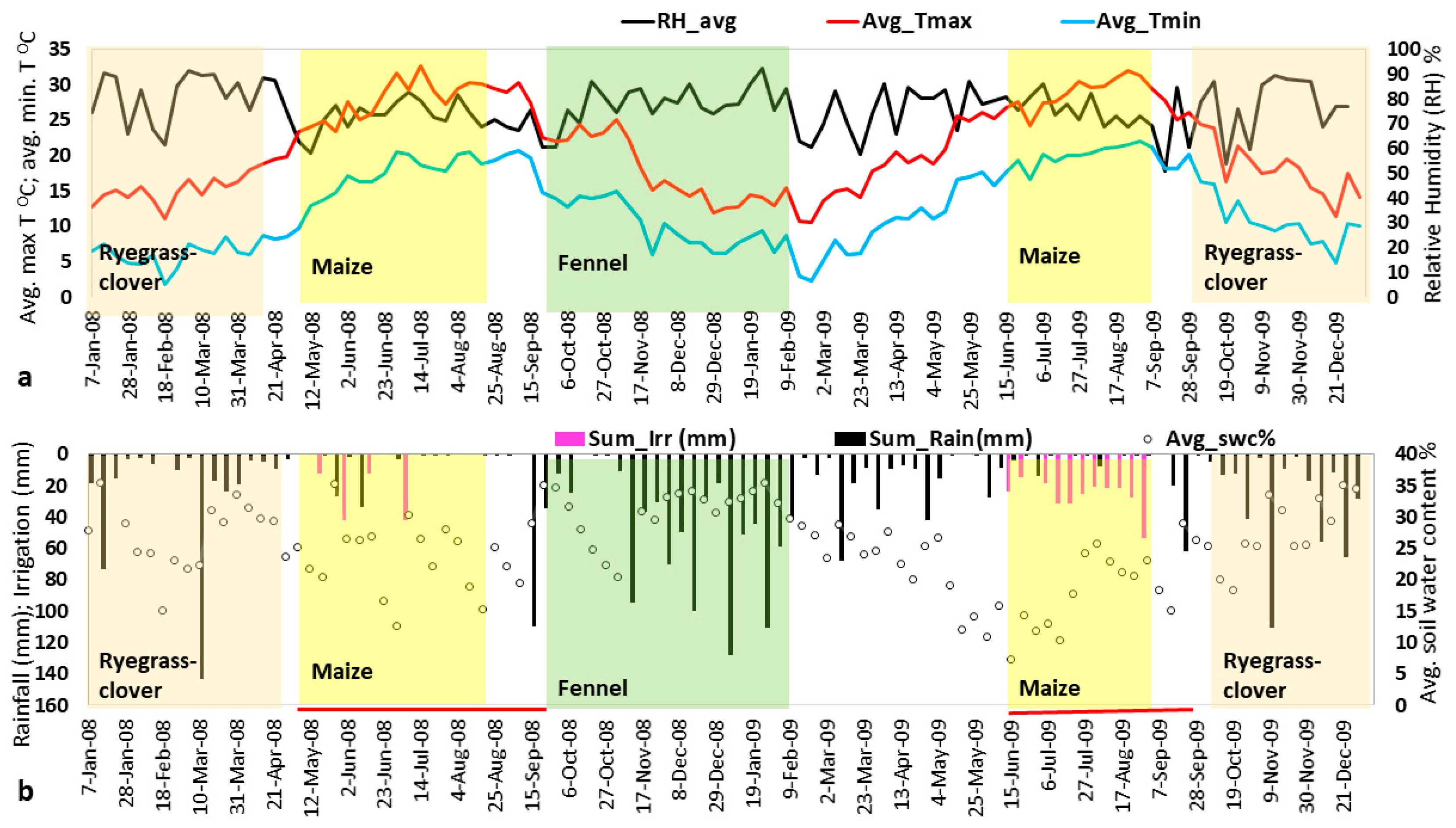
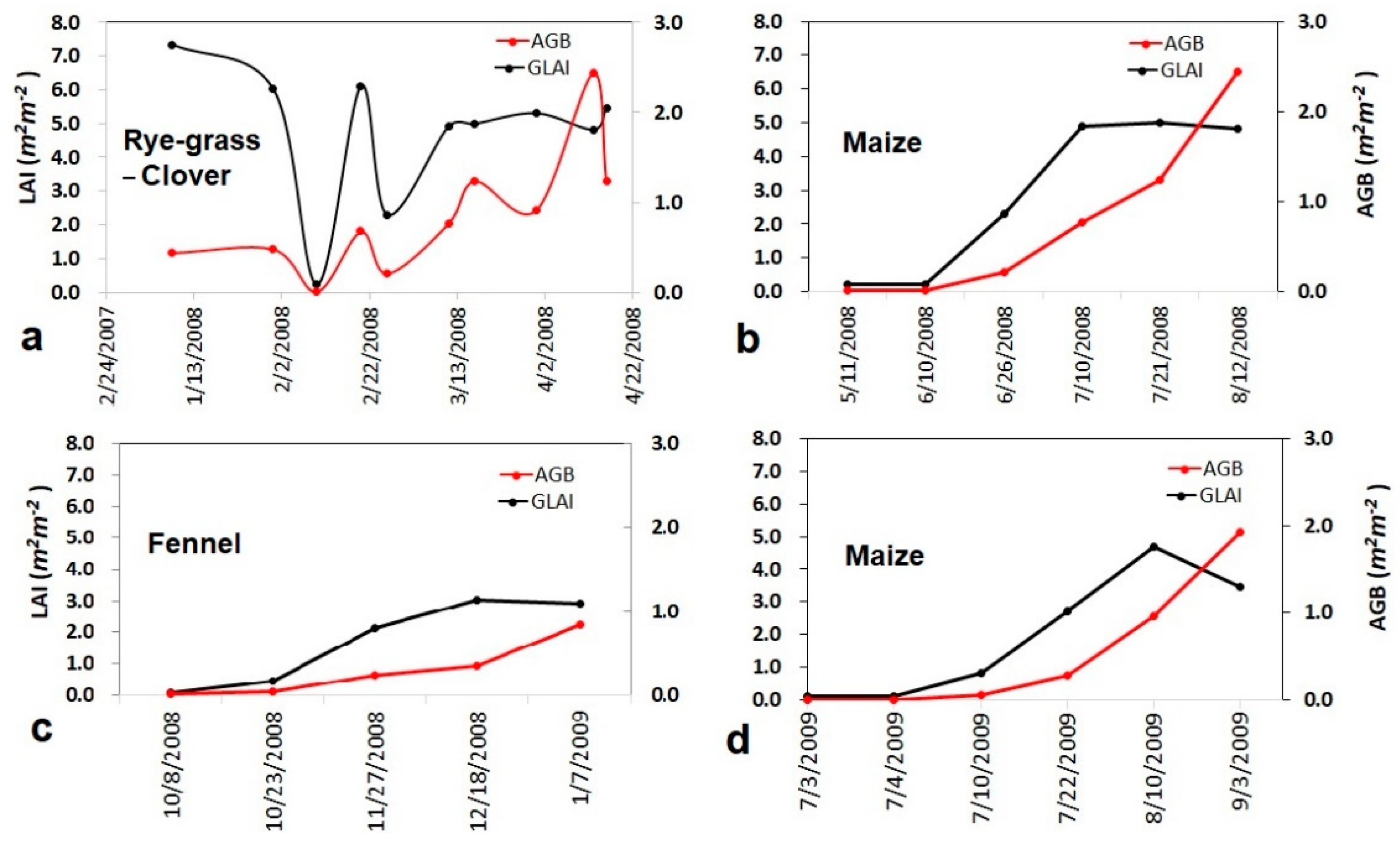
4.2. Irrigated Water Management and Crop Performance
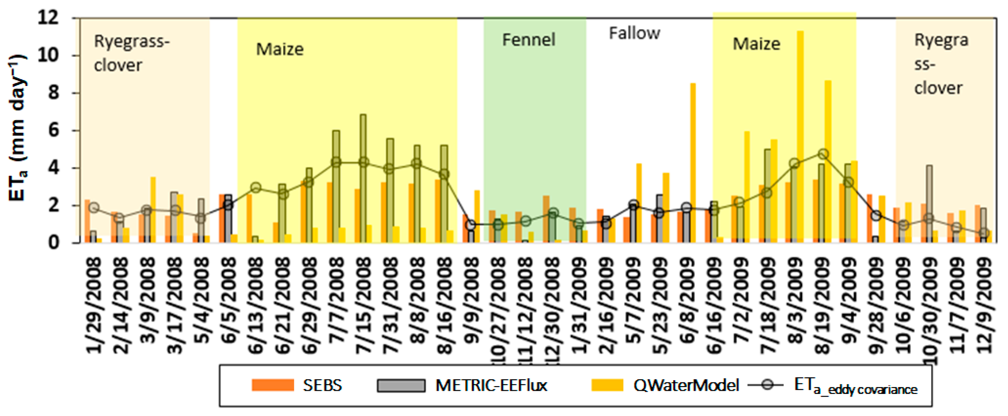
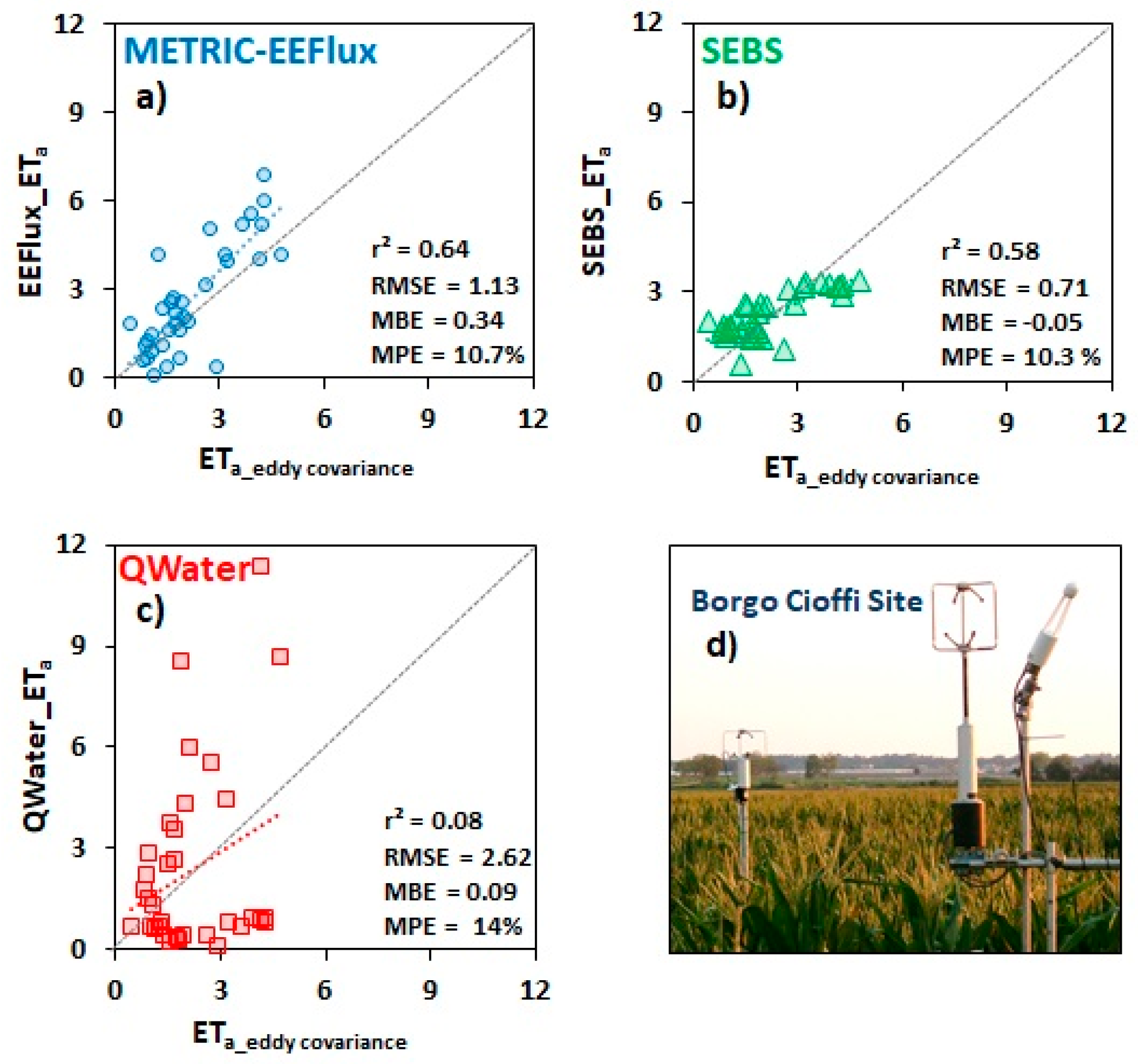
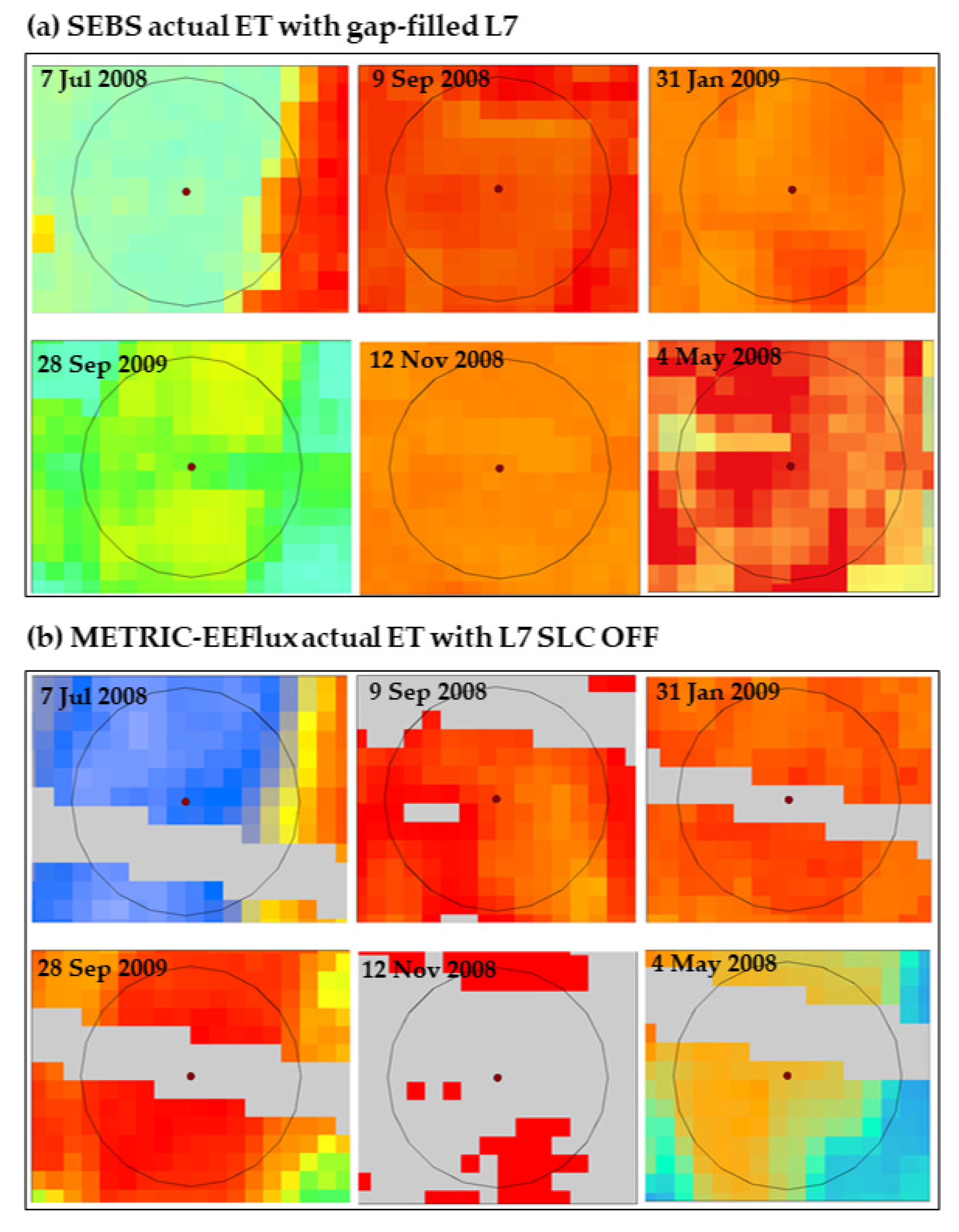
4.3. Evaluation of Model-Based Evapotranspiration
5. Conclusions
Supplementary Materials
Author Contributions
Funding
Data Availability Statement
Acknowledgments
Conflicts of Interest
References
- Oki, T.; Kanae, S. Global Hydrological Cycles and Freshwater Resources. Freshwater. Science 2006, 313, 1068–1073. [Google Scholar] [CrossRef] [PubMed] [Green Version]
- Fisher, J.B.; Melton, F.; Middleton, E.; Hain, C.; Anderson, M. The future of evapotranspiration: Global requirements for ecosystem functioning, carbon and climate feedbacks, agricultural management, and water resources. Water Resour. Res. 2017, 53, 2618–2626. [Google Scholar] [CrossRef]
- Milano, M.; Ruelland, D.; Fernandez, S.; Dezetter, A.; Fabre, J. Current state of Mediterranean water resources and future trends under climatic and anthropogenic changes. Hydrol. Sci. J. 2013, 58, 498–518. [Google Scholar] [CrossRef]
- Dury, J.; Schaller, N.; Garcia, F.; Reynaud, A.; Bergez, J.E. Models to support cropping plan and crop rotation decisions, A review. Agron. Sustain. Dev. 2012, 32, 567–580. [Google Scholar] [CrossRef] [Green Version]
- Govind, A.; Kumari, J. Understanding the terrestrial carbon cycle: An ecohydrological perspective. J. Ecol. 2014. [Google Scholar] [CrossRef] [Green Version]
- Govind, A.; Chen, J.M.; McDonnell, J.; Kumari, J.; Sonnentag, O. Effects of lateral hydrological processes on photosynthesis and evapotranspiration in a boreal ecosystem. Ecohydrology 2011, 4, 394–410. [Google Scholar] [CrossRef]
- Christou, A.; Dalias, P.; Neocleous, D. Spatial and temporal variations in evapotranspiration and net water requirements of typical Mediterranean crops on the island of Cyprus. J. Agric. Sci. 2017, 155, 1311–1323. [Google Scholar] [CrossRef]
- Khan, M.S.; Liaqat, U.W.; Baik, J.; Choi, M. Stand-alone uncertainty characterization of GLEAM, GLDAS and MOD16 evapotranspiration products using an extended triple collocation approach. Agric. For. Meteorol. 2018, 252, 256–268. [Google Scholar] [CrossRef]
- Blatchford, M.L.; Mannaerts, C.M.; Zeng, Y.; Nouri, H.; Karimi, P. Status of accuracy in remotely sensed and in-situ agricultural water productivity estimates: A review. Remote Sens. Environ. 2019, 234, 111413. [Google Scholar] [CrossRef]
- Paço, T.A.; Conceição, N.; Ferreira, M.I. Measurements and estimates of peach orchard evapotranspiration in Mediterranean conditions. Acta Hortic. 2004, 664, 505–512. [Google Scholar] [CrossRef]
- Alberto, M.C.R.; Wassmann, R.; Hirano, T.; Miyata, A.; Hatano, R. Comparisons of energy balance and evapotranspiration between flooded and aerobic rice fields in the Philippines. Agric. Water Manag. 2011, 98, 1417–1430. [Google Scholar] [CrossRef]
- Sugita, M.; Matsuno, A.; El-Kilani, R.M.M.; Abdel-Fattah, A.; Mahmoud, M.A. Crop evapotranspiration in the Nile Delta under different irrigation methods. Hydrol. Sci. J. 2017, 62, 1618–1635. [Google Scholar] [CrossRef] [Green Version]
- Liu, S.; Xu, Z. Micrometeorological Methods to Determine Evapotranspiration. Obs. Meas. Ecohydrol. Process. 2018. [Google Scholar] [CrossRef]
- Zitouna-Chebbi, R.; Prévot, L.; Chakhar, A.; Ben Abdallah, M.M.; Jacob, F. Observing actual evapotranspiration from flux tower eddy covariance measurements within a hilly watershed: Case study of the Kamech site, Cap Bon Peninsula, Tunisia. Atmosphere 2018, 9, 68. [Google Scholar] [CrossRef] [Green Version]
- Govind, A.; Cowling, S.; Kumari, J.; Rajan, N.; Al-Yaari, A. Distributed modeling of ecohydrological processes at high spatial resolution over a landscape having patches of managed forest stands and crop fields in SW Europe. Ecol. Modell. 2015, 297, 126–140. [Google Scholar] [CrossRef]
- Govind, A.; Chen, J.M.; Margolis, H.; Ju, W.; Sonnentag, O.; Giasson, M.A. A spatially explicit hydro-ecological modeling framework (BEPS-TerrainLab V2. 0): Model description and test in a boreal ecosystem in Eastern North America. J. Hydrol. 2009, 367, 200–216. [Google Scholar] [CrossRef]
- García-Tejero, I.F.; Hernández, A.; Rodríguez, V.M.; Ponce, J.R.; Ramos, V. Estimating almond crop coefficients and physiological response to water stress in semiarid environments (SW Spain). J. Agric. Sci. Technol. 2015, 17, 1255–1266. [Google Scholar]
- Samiha, O.; Noreldin, T.; Elsayed, M. “Et-Calculator” a New Model To Robustly Calculate Evapotranspiration in Egypt. J. Soil Sci. Agric. Eng. 2015, 6, 203–211. [Google Scholar] [CrossRef] [Green Version]
- Clarke, D.; Smith, M.; El-Askari, K. CropWat for Windows (Version 4.2); University of Southampton: Southampton, UK, 1998; p. 43. Available online: http://eprints.soton.ac.uk/73992/ (accessed on 1 February 2021).
- Albano, R.; Manfreda, S.; Celano, G. MY SIRR: Minimalist agro-hYdrological model for Sustainable IRRigation management—Soil moisture and crop dynamics. SoftwareX 2017, 6, 107–117. [Google Scholar] [CrossRef]
- Möller, M.; Stanhill, G. Hydrological impacts of changes in evapotranspiration and precipitation: Two case studies in semi-arid and humid climates. Hydrol. Sci. J. 2007, 52, 1216–1231. [Google Scholar] [CrossRef]
- de Teixeira, A.H.C.; Bastiaanssen, W.G.M. Five methods to interpret field measurements of energy fluxes over a micro-sprinkler-irrigated mango orchard. Irrig. Sci. 2012, 30, 13–28. [Google Scholar] [CrossRef] [Green Version]
- Khan, M.S.; Baik, J.; Choi, M. Inter-comparison of evapotranspiration datasets over heterogeneous landscapes across Australia. Adv. Sp. Res. 2020, 66, 533–545. [Google Scholar] [CrossRef]
- Er-Raki, S.; Chehbouni, A.; Guemouria, N.; Ezzahar, J.; Khabba, S. Citrus orchard evapotranspiration: Comparison between eddy covariance measurements and the FAO-56 approach estimates. Plant Biosyst. 2009, 143, 201–208. [Google Scholar] [CrossRef] [Green Version]
- Bhattarai, N.; Shaw, S.B.; Quackenbush, L.J.; Im, J.; Niraula, R. Evaluating five remote sensing based single-source surface energy balance models for estimating daily evapotranspiration in a humid subtropical climate. Int. J. Appl. Earth Obs. Geoinf. 2016, 49, 75–86. [Google Scholar] [CrossRef]
- Olivera-Guerra, L.; Merlin, O.; Er-Raki, S.; Khabba, S.; Escorihuela, M.J. Estimating the water budget components of irrigated crops: Combining the FAO-56 dual crop coefficient with surface temperature and vegetation index data. Agric. Water Manag. 2018, 208, 120–131. [Google Scholar] [CrossRef] [Green Version]
- Senay, G.B.; Bohms, S.; Singh, R.K.; Gowda, P.H.; Velpuri, N.M. Operational Evapotranspiration Mapping Using Remote Sensing and Weather Datasets: A New Parameterization for the SSEB Approach. J. Am. Water Resour. Assoc. 2013, 49, 577–591. [Google Scholar] [CrossRef] [Green Version]
- de Oliveira Costa, J.; José, J.V.; Wolff, W.; de Oliveira, N.P.R.; Oliveira, R.C. Spatial variability quantification of maize water consumption based on Google EEflux tool. Agric. Water Manag. 2020, 232. [Google Scholar] [CrossRef]
- Allen, R.; Irmak, A.; Trezza, R.; Hendrickx, J.M.H.; Bastiaanssen, W. Satellite-based ET estimation in agriculture using SEBAL and METRIC. Hydrol. Process. 2011, 25, 4011–4027. [Google Scholar] [CrossRef]
- Al-Bakri, J.T. Crop mapping and validation of ALEXI-ET in Azraq and Mafraq areas. In A Report for Regional Coordination on Improved Water Resources Management and Capacity Building; Ministry of Water and Irrigation: Amman, Jordan, 2015. [Google Scholar]
- Ma, W.; Hafeez, M.; Rabbani, U.; Ishikawa, H.; Ma, Y. Retrieved actual ET using SEBS model from Landsat-5 TM data for irrigation area of Australia. Atmos. Environ. 2012, 59, 408–414. [Google Scholar] [CrossRef]
- Khan, M.S.; Baik, J.; Choi, M. A physical-based two-source evapotranspiration model with Monin-Obukhov similarity theory. GIsci. Remote Sens. 2021, 1–32. [Google Scholar] [CrossRef]
- Samuel, A.; Girma, A.; Zenebe, A.; Ghebreyohannes, T. Spatio-temporal variability of evapotranspiration and crop water requirement from space. J. Hydrol. 2018, 567, 732–742. [Google Scholar] [CrossRef]
- French, A.N.; Jacob, F.; Anderson, M.C.; Kustas, W.P.; Timmermans, W. Surface energy fluxes with the Advanced Spaceborne Thermal Emission and Reflection radiometer (ASTER) at the Iowa 2002 SMACEX site (USA). Remote Sens. Environ. 2005, 99, 55–65. [Google Scholar] [CrossRef]
- Timmermans, W.J.; Van Der Kwast, J.; Gieske, A.S.; Su, Z.; Olioso, A. Intercomparison of Energy Flux Models Using ASTER Imagery at the SPARC 2004 Site. In Proceedings of the ESA WPP-250: SPARC Final Workshop, Barrax, Spain, 12–14 July 2003; pp. 4–5. [Google Scholar]
- Vitale, L.; Di Tommasi, P.; D’Urso, G.; Magliulo, V. The response of ecosystem carbon fluxes to LAI and environmental drivers in a maize crop grown in two contrasting seasons. Int. J. Biometeorol. 2016, 60, 411–420. [Google Scholar] [CrossRef] [PubMed] [Green Version]
- Twine, T.E.; Kustas, W.P.; Norman, J.M.; Cook, D.R.; Houser, P.R. Correcting eddy-covariance flux underestimates over a grassland. Agric. For. Meteorol. 2000, 103, 279–300. [Google Scholar] [CrossRef] [Green Version]
- Bowen, I.S. The ratio of heat losses by conduction and by evaporation from any water surface. Phys. Rev. 1926, 27, 779–787. [Google Scholar] [CrossRef] [Green Version]
- Walter, I.A.; Allen, R.G.; Elliott, R.; Jensen, M.E.; Itenfisu, D.; Mecham, B.; Howell, T.A.; Snyder, R.; Brown, P.; Echings, S.; et al. ASCE’s standardized reference evapotranspiration equation. In Proceedings of the Watershed Management and Operations Management, Fort Collins, CO, USA, 20–24 June 2000; ASCE Library: Reston, VA, USA, 2000; pp. 1–11. [Google Scholar]
- Chander, G.; Markham, B.L.; Helder, D.L. Summary of current radiometric calibration coefficients for Landsat MSS, TM, ETM+, and EO-1 ALI sensors. Remote Sens. Environ. 2009, 113, 893–903. [Google Scholar] [CrossRef]
- Desai, M.; Ganatra, A. Survey on Gap Filling in Satellite Images and Inpainting Algorithm. Int. J. Comput. Theory Eng. 2012, 4, 341–345. [Google Scholar] [CrossRef]
- Zhang, C.; Li, W.; Civco, D. Application of geographically weighted regression to fill gaps in SLC-off Landsat ETM+ satellite imagery. Int. J. Remote Sens. 2014, 35, 7650–7672. [Google Scholar] [CrossRef]
- Liang, S. Narrowband to broadband conversions of land surface albedo I: Algorithms. Remote Sens. Environ. 2001, 76, 213–238. [Google Scholar] [CrossRef]
- Smith, R.B. The Heat Budget of the Earth’s Surface Deduced from Space; Yale University Center for Earth Observation: New Haven, CT, USA, 2010. [Google Scholar]
- Valor, E.; Caselles, V. Mapping land surface emissivity from NDVI: Application to European, African, and South American areas. Remote Sens. Environ. 1996, 57, 167–184. [Google Scholar] [CrossRef]
- Farr, T.; Rosen, P.; Caro, E. The Shuttle Radar Topography Mission. Rev. Geophys. 2007, 45, RG2004. [Google Scholar] [CrossRef] [Green Version]
- Reichstein, M.; Falge, E.; Baldocchi, D.; Papale, D.; Aubinet, M. On the separation of net ecosystem exchange into assimilation and ecosystem respiration: Review and improved algorithm. Glob. Chang. Biol. 2005, 11, 1424–1439. [Google Scholar] [CrossRef]
- Geerts, S.; Raes, D. Deficit irrigation as an on-farm strategy to maximize crop water productivity in dry areas. Agric. Water Manag. 2009, 96, 1275–1284. [Google Scholar] [CrossRef] [Green Version]
- Allen, R.G.; Tasumi, M.; Morse, A.; Trezza, R.; Wright, J.L. Satellite-Based Energy Balance for Mapping Evapotranspiration with Internalized Calibration (METRIC)—Applications. J. Irrig. Drain. Eng. 2007, 133, 395–406. [Google Scholar] [CrossRef]
- Laounia, N.; Abderrahmane, H.; Abdelkader, K.; Zahira, S.; Mansour, Z. Evapotranspiration and Surface Energy Fluxes Estimation Using the Landsat-7 Enhanced Thematic Mapper Plus Image over a Semiarid Agrosystem in the North-West of Algeria. Rev. Bras. Meteorol. 2017, 32, 691–702. [Google Scholar] [CrossRef] [Green Version]
- Hamimed, A.; Zaagane, M. Assessing Evapotranspiration and Drought Stress over a Semiarid Agricultural Area in Algeria with RS Data. Int. J. Water Resour. Arid. Environ. 2017, 6, 58–64. [Google Scholar]
- Su, Z.; Schmugge, T.; Kustas, W.P.; Massman, W.J. An evaluation of two models for estimation of the roughness height for heat transfer between the land surface and the atmosphere. J. Appl. Meteorol. 2001, 40, 1933–1951. [Google Scholar] [CrossRef] [Green Version]
- Karssenberg, D.; de Jong, K.; van der Kwast, J. Modelling landscape dynamics with Python. Int. J. Geogr. Inf. Sci. 2007, 21, 483–495. [Google Scholar] [CrossRef]
- Van Der Kwast, J.; Timmermans, W.; Gieske, A.; Su, Z.; Olioso, A. Evaluation of the Surface Energy Balance System (SEBS) applied to ASTER imagery with flux-measurements at the SPARC 2004 site (Barrax, Spain). Hydrol. Earth Syst. Sci. 2009, 13, 1337–1347. [Google Scholar] [CrossRef] [Green Version]
- Timmermans, W.J.; Kustas, W.P.; Andreu, A. Utility of an Automated Thermal-Based Approach for Monitoring Evapotranspiration. Acta Geophys. 2015, 63, 1571–1608. [Google Scholar] [CrossRef] [Green Version]
- Ellsäßer, F.; Röll, A.; Stiegler, C.; Hölscher, D. Introducing QWaterModelModel, a QGIS plugin for predicting evapotranspiration from land surface temperatures. Environ. Model. Softw. 2020, 130. [Google Scholar] [CrossRef]
- Ayyad, S.; Al Zayed, I.S.; Ha, V.T.T.; Ribbe, L. The performance of satellite-based actual evapotranspiration products and the assessment of irrigation efficiency in Egypt. Water 2019, 11, 1913. [Google Scholar] [CrossRef] [Green Version]
- Swelam, A.; Govind, A.; Abdallah, M.; Steduto, P.; Taha, A. Validation of remote-sensing evapotranspiration data of selected crops in the nile delta. In Proceedings of the 3rd World Irrigation Forum (WIF3), Bali, Indonesia, 1–7 September 2019. [Google Scholar]


| Instrument | Field Measurements |
|---|---|
| Eppley Laboratory Inc., Newport, RI, USA | Incident and reflected global radiation (4 m) |
| Rebs Q7.1, Seattle, WA, USA | Net radiation (4 m) |
| LI-190SA, LI-COR Inc., Lincoln, NE, USA, Rotronic MP, Campbell Sci. Ltd., Shepshed, UK | Incident and reflected photo-synthetically active radiation, air temperature and relative humidity (4 m) |
| Sonic anemometer R3 (Gill Instruments Ltd., Lymington, UK) | Wind speed and direction (4 m) |
| Rain Collector II, Davis Instruments, Hayward, CA, USA | Precipitation and irrigation (ground level) |
| TCAV thermocouple probes | Soil temperature (0.3 m depth) |
| CS water content reflectometer (Campbell Scientific, Ltd., Shepshed, UK) | Volumetric soil water content (SWC)—(0.3 m depth) |
| Variables | Equations |
|---|---|
| Albedo | |
| NDVI | |
| Fractional Cover | |
| Emissivity |
| Crop | ETa (mm) | Irrigation (mm) | Rain (mm) | Rainy Days | Duration |
|---|---|---|---|---|---|
| Maize 2008 | 305.41 | 34.21 | 68.59 | 18.00 | 1 May–22 August 2008 |
| Fennel 2008–2009 | 179.61 | 0.00 | 924.67 | 88.00 | 15 September 2008–5 February 2009 |
| Maize 2009 | 275.90 | 291.60 | 24.90 | 17.00 | 11 June–8 September 2009 |
| All crops | 1336.88 | 399.58 | 2966.35 | 309.00 | 1 January 2008–31 December 2009 |
| Crop | GPP (g cm−2) | AGB (m2m−2) | Max Yield (kg m−2) | WUE (kgha−1mm−1) | Canopy Height (m) | Max LAI (m2m−2) |
|---|---|---|---|---|---|---|
| Maize 2008 | 9.55 | 2.44 | 1171.30 | 5.20–30.00 | 0.31–2.95 | 4.98 |
| Fennel 2008–2009 | 2.41 | 0.87 | 406.39 | 6.80–36.40 | 0.10–0.80 | 3.00 |
| Maize 2009 | 8.20 | 1.92 | 923.50 | 3.60–34.00 | 0.26–2.64 | 4.80 |
Publisher’s Note: MDPI stays neutral with regard to jurisdictional claims in published maps and institutional affiliations. |
© 2021 by the authors. Licensee MDPI, Basel, Switzerland. This article is an open access article distributed under the terms and conditions of the Creative Commons Attribution (CC BY) license (http://creativecommons.org/licenses/by/4.0/).
Share and Cite
Nisa, Z.; Khan, M.S.; Govind, A.; Marchetti, M.; Lasserre, B.; Magliulo, E.; Manco, A. Evaluation of SEBS, METRIC-EEFlux, and QWaterModel Actual Evapotranspiration for a Mediterranean Cropping System in Southern Italy. Agronomy 2021, 11, 345. https://doi.org/10.3390/agronomy11020345
Nisa Z, Khan MS, Govind A, Marchetti M, Lasserre B, Magliulo E, Manco A. Evaluation of SEBS, METRIC-EEFlux, and QWaterModel Actual Evapotranspiration for a Mediterranean Cropping System in Southern Italy. Agronomy. 2021; 11(2):345. https://doi.org/10.3390/agronomy11020345
Chicago/Turabian StyleNisa, Zaibun, Muhammad Sarfraz Khan, Ajit Govind, Marco Marchetti, Bruno Lasserre, Enzo Magliulo, and Antonio Manco. 2021. "Evaluation of SEBS, METRIC-EEFlux, and QWaterModel Actual Evapotranspiration for a Mediterranean Cropping System in Southern Italy" Agronomy 11, no. 2: 345. https://doi.org/10.3390/agronomy11020345