Simulated Climate Change Impacts on Corn and Soybean Yields in Buchanan County, Iowa

Abstract

Projections of climate patterns through the end of the 21st century indicate varying impacts across the U.S. However, a common thread of these projections calls for increasing atmospheric temperatures in every region, some more pronounced than others. The significance of these projections for corn and soybean production cannot be overestimated. This study contributes to our understanding of climate change impacts on production and farm revenues by projecting their impacts on corn and soybean yields in Buchanan County, Iowa, a county in the center of the Corn Belt. Projections indicate that as atmospheric temperatures rise and precipitation levels vary markedly, the result is a significant decline in corn and soybean yields, the latter to a lesser extent, as compared to long-term yield trends. Depending upon the climate change scenario that will materialize, corn yields are projected to decline by up to 29%, while soybean yields are projected to decline by up to 24% from their normal upward trends by the year 2100. Due to the long-term upward trends in yields, corn and soybean yields will increase in absolute terms by the end of the century. Depending upon the climate change scenario, actual corn and soybean yields will increase by 30 to 57% and 30 to 66%, respectively, by the end of the 21st century, significantly less than they would have in the absence of these climate projections.

1. Introduction

Iowa is the top corn-producing state in the U.S. and consistently ranks either first or second in soybean production. As a result, the state plays a major role in national and global food and fiber markets. About 90 percent of the land in the state is utilized for agriculture, dominated by corn and soybean production [1]. Given the dominance of agriculture in general, and corn (Zea mays L.) and soybeans (Glycine max L.) in particular, any significant changes in the production of these two crops due to changes in ambient factors such as climate will impact the agricultural sector domestically and globally. The impact of potential changes in weather patterns on crop and livestock production and farm incomes has received some attention in the literature, e.g., [2,3,4]. The primary climate variables of interest are precipitation and temperature, though other weather variables such as solar radiation and wind speed also play noticeable roles.

In the Midwestern states of the U.S., the average air temperature increased by more than 1.5 degrees F between 1910 and 2010 [5]. Various studies indicate that there has been a large increase in the number of days of heavy rainfall while total annual precipitation levels remain largely unchanged. Heavy rains predispose to soil erosion and loss of nutrients, while increasing the costs of field operations due to heavy moisture conditions [6]. Increased precipitation could also increase the infestation of pests and disease, and water clogging conditions, particularly in clayey soils.

Various studies indicate that future crop yields will be highly predicated upon extreme weather events [5]. For instance, wetter springs would delay planting, leading to the necessity to utilize shorter-season varieties. Consequently, the distribution of temperature and precipitation and other pertinent weather variables will play a key role in the future patterns of production and incomes.

The relationship between crop yields and climate/weather is well documented, e.g., [7]. For example, Hatfield and Prueger [7] indicated how extreme temperatures impact plant growth by adding stress to plants, thus reducing yield potential [7,8,9]. Hatfield and Prueger [7] further recognized that increased CO₂ levels promote weeds and that other climate changes such as high humidity levels promote diseases and insect growth. In addition, studies in the academic literature have documented that agricultural production is strongly correlated with biophysical attributes of farms in addition to weather and management practices, e.g., [10,11,12]. It is thus not surprising that the projected changes in climate patterns are being received with apprehension among the scientific community.

More apropos to climate change and corn production, Schlenker and Roberts [2] found using regression models that corn yields are projected to decline by about 40% under the mildest warming scenario and as much as 80% under the most rapid warming scenario. They found soybean yields may also be impacted, but not quite as much—about 30% under the mildest scenario and about 70% under the most rapid warming scenario. In contrast, Parajulia et al. [13], using the Soil and Water Assessment Tool (SWAT) ecohydrological model [14,15,16], did not find any significant decline in corn or soybean yields under climate change in the Big Sunflower watershed in Mississippi. In fact, they found that the impacts on corn yields may range from a reduction of 12% to an increase of 34%, while soybean yields may increase by up to 12.5% or decrease by up to 16.6%. The discrepancy between some of the reported impacts is attributable in part to the methodology used. Regression models, however complex, are not as capable of reflecting the complex mechanistic relationships between crop growth and productivity as compared to SWAT and the Agricultural Policy Environmental eXtender (APEX) ecohydrological models [16,17,18].

Dell et al. [12] studied the extent to which climate change has impacted various economic outcomes, including economic impacts on the agricultural sector. In that study, as in most others, the primary weather-related inputs include precipitation rates, minimum and maximum temperatures, and humidity levels, which often serve as inputs in production functions. Other studies have also used cross-sectional regressions, utilizing panel data and applying a hedonic approach (as in Lambert [11], which included key weather variables). These studies confirmed that adverse weather negatively impacted U.S. agriculture. Similar results were observed in studies covering India, Mexico, and Indonesia. While crop insurance payments buffer farmers from revenue losses, these offsets of price movements nonetheless have to be shouldered by taxpayers via government payments.

Schlenker and Roberts [2], examining temperature data and plant growth, discovered optimum temperatures in output yields ranging from 29 to 32 °C. They also discovered that the relationship between temperature and agricultural output is often nonlinear. The ideal temperatures vary from one crop to another; for example, for corn, it is 29 °C; for soybeans, it is 30 °C; while for cotton it is 32 °C. Temperatures within the optimal range are most conducive to plant growth and productivity. However, even a small increase above the threshold levels significantly reduces output yields. Thus, the relationship between temperature and yields follows a non-linear path.

Changes in precipitation levels also impact yields, particularly for rain-fed crops. For example, in Mexico (whose agriculture is highly dependent on rainfall), warmer and dryer conditions have substantial nutritional and economic implications. Even with irrigation reservoirs, water can become scarce under dryer conditions [19]. In addition, dry and warmer climates in agricultural regions heighten the exodus of farm workers to urban areas [20]. In general, high levels of rainfall lead to higher yields, and vice versa [21,22].

The foregoing discussion relates to short-term implications. Some economists have argued that in the long run, adaptation and mitigation methods such as utilization of drought-resistant crops and other adaptive management practices such as conservation tillage could mitigate the impacts of short-run weather fluctuations [23]. Nevertheless, long-run impacts of climate change are likely to adversely impact agriculture output. Previous discussions regarding changes in climate patterns have raised interest in opposing opinions regarding whether these changes are caused by natural geological forces or anthropogenic factors. Notwithstanding the inconclusive nature of climate change viewpoints, substantial efforts have been expended to forecasting weather patterns into the future. Projections of daily weather data are available through the end of the 21st century from a wide ensemble of global climate models. From a food security standpoint, what is most pertinent is the implications of these projections for the distribution of food production and farm incomes.

While forecasted variabilities in climate are likely to impact food and fiber production and have significant implications for U.S. policy and food security, the specific impacts have not been adequately quantified. However, the conclusions from recent studies provide clear indications about general expectations. For instance [24,25], indicate with a high degree of confidence that climate change impacts have already slowed agricultural productivity and will continue to impede food availability and nutritional quality, especially under the Representative Concentration Pathway (RCP) 8.5 scenario, unless checked by robust mitigation measures. Besides its well-documented impacts on the general availability of food, climate change has also been projected to impact food safety [26].

The research we have conducted here is focused on providing insight into the likely impacts on corn and soybean yields in Iowa, which is a leading U.S. producer of both crops [27]. We use widely accredited compilations of climate projections to determine the likely impacts on corn and soybean yields assuming that current market conditions and crop production (genetic) potential hold. For this purpose, we use the well-tested and calibrated APEX ecohydrological model [28,29] to estimate climate change impacts on crop yields and production levels. Gassman et al. [28] documented extensive hydrologic and pollutant-transport testing in their review of (1) APEX applications for livestock production scenarios in Texas and Iowa, and (2) cropland conditions in Iowa, Missouri, and Texas, forested conditions in Texas, and other landscapes in North Dakota, Texas, and China. Expanded use of APEX has since been reported in the more recent literature, including applications focused on evapotranspiration [30,31], corn yields, and water balance [32], rainfall distribution and snowmelt [33], forage production [34], soybean–rice production and irrigation strategies [35], climate change [36,37,38], and phosphorus transport in subsurface tile drains [39]. Recent studies also describe modified versions of APEX for bacteria transport [40], rice paddy dynamics [41,42,43], and groundwater interactions via an interface with the MODFLOW model [44].

We employ APEX in this study to determine the most plausible future trajectory of corn and soybean yields in a northeastern county in Iowa, where the model has been successfully calibrated to simulate crop yields and the impacts of various conservation practices [45]. We also shed light on potential yields by incorporating the effects of the long-term trajectory of corn and soybean yields, an aspect that is largely absent from previous studies. The results of this study indicate the extent to which current production levels and counter-cyclical farm income support programs will be subject to significant stresses if the projections of warmer weather patterns materialize.

2. Materials and Methods

2.1. Modeling System

APEX [17] is a comprehensive field-scale model that was developed to assess the effects of management strategies on a broad spectrum of agronomic and ecological indicators such as crop growth and yields, livestock grazing, and water quality. APEX is specifically designed for whole-farm or small-watershed analyses and is a modified version of the Erosion Productivity Impact Calculator (EPIC; [46,47]) model that has also been used widely to simulate alternative management scenarios such as variations in manure and fertilizer application rates, mode and timing, alternative tillage practices, structural controls, and other cultural management practices. Model components include weather, hydrology, soil temperature, grazing, erosion-sedimentation, nutrient and carbon cycling, tillage, dairy management practices, crop management and growth, fate and transport of pesticide and nutrients, and costs and returns of various management practices.

APEX operates on a daily time step and can be applied for a wide range of soil, landscape, climate, crop rotation, and management practice combinations. A key advantage is its ability to simulate up to ten types of vegetation growing concurrently on the same subarea. APEX can be executed for a single field or for a wide range of multi-field configurations including whole farms or small watersheds. APEX is detailed enough to simulate precise management practices such as filter strip impacts on nutrient and chemical transport from application fields. The model permits input of simulated cropping system, manure and/or fertilizer nutrient characteristics, tillage practices, soil layer properties, and other characteristics for each subarea. Key model outputs include crop yields, edge-of-field nutrient and sediment losses, and other water and nutrient balance indicators.

APEX has also been calibrated against annual county-level crop yield data that is available through the USDA National Agricultural Statistics Service (USDA-NASS) [1]. The model is included in USDA’s web-based Nutrient Tracking Tool (NTT) [48] and has been calibrated extensively for various applications to assess edge-of-field water quality impacts across a wide variety of land uses in the U.S. and other nations, e.g., [28]. APEX was calibrated against historical weather and agricultural production data in a prior application to the upper Maquoketa River watershed (UMRW) in northeastern Iowa [45]. For this study, APEX was validated for Buchanan County—which covers a portion of the UMRW in Iowa—using available crop yield and edge-of-field water quality measurements. APEX was then used to estimate crop yields under future climate patterns.

2.2. Data Sources

A number of data sources were used for this study. Many of the following datasets are also incorporated into the web-based NTT tool. Others were specifically assembled for this study. Various Geographic Information Systems (GIS) data layers—as specified below—were overlaid in order to determine the distribution of corn- and soybean-growing areas in Buchanan County, Iowa. Key data used were the cropland data layer for 2021, soils data, weather data (historical as well as future climate projections), and crop management data.

2.2.1. Cropland Data Layer (CDL)

A 20-year GIS history of cropland cover for Buchanan County, Iowa, was obtained from the USDA-NRCS CDL data server [49]. For this study, the corn and soybean layers for 2021, the most recent layer, were used. The CDL data are available at a 30 m level of precision, and this level of precision was used to identify fields on which corn and soybeans were planted in 2021. For the continuous corn results reported here, simulations were restricted only to fields used for corn in 2021. For the corn following soybean and soybean results, simulations were performed on fields used for corn or soybeans.

2.2.2. Soils Data

The USDA-NRCS Soil Survey Geographic Database (SSURGO) [50] for each survey area have been assembled for the conterminous U.S.. For this study, the SSURGO data layer was overlaid on the CDL data in order to determine the soil types applicable to 2021 corn and soybean fields in Buchanan County, Iowa. A total of over 88,322 unique crop–soil polygons were identified as corn-growing land parcels within Buchanan County, Iowa for 2021. Similarly, a total of 69,651 crop–soil polygons were identified as soybean-growing fields within the county. The 88,322 polygons were utilized for continuous corn simulations while the combined total of 157,973 polygons were used for soybean and corn following soybean simulations.

2.2.3. Crop Management Data

Field operations and nutrient application rates for continuous corn and corn–soybean rotations were obtained from producers as part of the UMRW application [45,51,52]. Baseline crop management represented a reduced tillage system. These specific baseline field operations were used for the simulations for model validation purposes, and are presented below.

Continuous corn field operations: Based on producer input received as part of the UMRW study [51], the field operations performed on continuous corn fields under status quo management are listed in

Table 1. Field operations simulated for continuous corn for 1998–2000 production years.

Date	Operation *
16 April	Apply manure (44.9 MT/ha)
29 April	Apply herbicide
1 May	Field cultivate
3 May	Plant
3 May	Incorporate starter fertilizer (kg/ha) (10.1 + 11.3 + 27.9)
12 June	Cultivate
18 October	Harvest corn
23 October	Bulk spread (kg/ha) (17.9 + 20.2 + 41.9)
2 November	Chisel plow
12 November	Apply ammonia (194.2 kg/ha)

* The data in this table represent operations on fields receiving manure. For fields not receiving manure, the only differences were as follows: the manure application operation was excluded and bulk-spread operation on 23 October was changed to 28.0 + 30.0 + 55.8.

. Fertilizer nutrient application rates on fields receiving manure were notably different than on fields not receiving manure. To reflect the varied practices on fields receiving manure versus those not receiving manure, climate scenario simulations were performed for manure-receiving fields and subsequently replicated for fields not receiving manure. Based on Osei et al. [51], about 15.6% of cropland area received manure while the remainder did not. Consequently, the final results analyzed represented a weighted average, using weights of 15.6% and 84.4%, respectively, for manure and non-manure field simulations. Status quo tillage practices (presented in Table 1) represented a reduced-tillage style of management.

Corn–soybean field operations: Similar to the foregoing, producer input received as part of the UMRW study [51] resulted in the field operations presented in

Table 2. Field operations simulated for corn–soybean rotation for 1998–2000 production years *.

Date	Operation
	Corn following soybean
16 April	Apply manure (44.9 MT/ha)
29 April	Apply herbicide
29 April	Apply fertilizer N (128.2 kg/ha)
30 April	Field cultivate
1 May	Plant corn
1 May	Incorporate starter fertilizer (kg/ha) (10.1 + 11.3 + 27.9)
12 June	Cultivate
15 October	Harvest corn
25 October	Bulk spread (kg/ha) (17.9 + 20.2 + 41.9)
1 November	Chisel plow
	Soybean following corn
16 April	Apply manure (44.9 MT/ha)
29 April	Apply herbicide
10 May	Field cultivate
12 May	Plant soybean
2O ctober	Harvest soybean
27 October	Bulk spread (kg/ha) (15.4 + 17.3 + 41.9)

* The data in this table represent operations on fields receiving manure. For fields not receiving manure, the only differences simulated were as follows: the manure application operations were excluded and the bulk-spread application rates were changed to 28.0 + 30.1 + 55.8 for corn and soybeans.

for corn–soybean fields under status quo management. Fertilizer nutrient application rates on fields receiving manure are once again different than on fields not receiving manure. Simulations were performed for fields receiving manure, as well as fields where only inorganic fertilizer was utilized as the nutrient source. Status quo tillage practices represented a reduced-tillage style of management.

For the two-year corn–soybean rotation, each polygon was divided into two equal halves, one starting in the corn year and the other starting in the soybean year, in order to ensure that each crop was simulated in each year so as to obtain an accurate weather representation for all crops. Polygon divisions were accomplished in the APEX subarea file prior to each simulation by assigning a negative sign to the second subarea, thus specifying side-by-side addition rather than routing from one half to the other.

In addition to the baseline management practices, simulations were replicated using current crop management practices relevant for the 2020–2021 period to better reflect current crop productivity in order to cast crop yield forecasts in a more relevant context. The results of these yield impacts are also presented in this paper. Crop management information were assumed to be exogenous and to follow the baseline practices specified above. Furthermore, for validation purposes, crop productivity was assumed to remain static at 1998–2000 levels. In particular, the crop parameters utilized for the upper Maquoketa River watershed study [45,52] were utilized for this study. An additional set of simulations was performed using current crop management and yield potential—applicable to the 1999–2021 period—once model validation tests were successful. The output from these additional simulations are also presented in the Results and Discussion section below.

2.2.4. Historical Weather Data

Historical data on key weather variables such as precipitation and minimum and maximum temperature were obtained from the USDA Parameter-elevation Regressions on Independent Slopes Model (PRISM) [53] database. For this study, the 4 km resolution of PRISM data was used. These data represent the baseline weather against which climate projections were compared. The simulations presented here were performed with a 25-year time horizon for the baseline and all climate projections. The specific baseline scenario for model validation was represented by the PRISM weather time series covering the 1981–2005 period. Another baseline—for crop yield forecasting—was represented by the 1996–2020 PRISM weather data to more closely reflect current weather.

2.3. Climate Projections

Data on climate projections were assembled from the National Center for Atmospheric Research (NCAR)’s Earth System Grid portal [54,55]. For this study, the climate projection data included daily time series on precipitation, minimum temperature, and maximum temperature that are available for the period of 2006 through 2099. Specific climate projections used were the downscaled Coupled Model Intercomparison Project—Phase 5 (CMIP 5) weather projections [56,57] from NCAR and the Lawrence Livermore National Laboratory. The NCAR data were obtained from the Bureau of Land Reclamation server at a one-eighth degree latitude and longitude grid for the entire conterminous United States. For climate scenario simulations, climate grid points were associated with each crop–soil polygon simulated simply by proximity, based on the Euclidean distance between the climate grid point and the geographic centroid of the crop–soil polygon.

The predominantly used climate projections are based on one of four Intergovernmental Panel on Climate Change (IPCC) scenarios depending on assumptions about greenhouse gas (GHG) emissions. Each climate change scenario used in this study is based on a representative concentration pathway (RCP) that represents a trajectory of GHG concentrations anticipated in response to corresponding mitigation assumptions. The four main RCPs (RCP2.6, RCP4.5, RCP6.0, and RCP8.5) adopted by the IPCC have been widely used in climate projections. Of the four RCP scenarios, three were used for this study, representing a middle ground (RCP4.5), an approximate average of a best-case lower emissions scenario (RCP2.6), and an opposite scenario which assumes that the current greenhouse gas emissions trajectory would be maintained (RCP8.5).

The nomenclature of the RCPs corresponds to projected radiative forcing values—expressed in Watts per square meter (Wm⁻²)—by 2100 under these scenarios as compared to the preindustrial era. RCP2.6, the most optimistic among the four for reducing global warming, corresponds to a radiative forcing of 2.6 Wm⁻² as compared to pre-industrial-era values, and is projected to result in a 1 °C increase in mean global temperatures by the mid-century (2046 to 2065) period. Similarly, RCP4.5 and RCP8.5 correspond to radiative forcing values of 4.5 Wm⁻² and 8.5 Wm⁻², respectively, as compared to the pre-industrial era and are projected to result, respectively, in 1.4 °C and 2.0 °C increases in mean global temperatures by the mid-century period. RCP8.5 represents the most pessimistic scenario among the four for reducing global warming.

Daily weather data on precipitation and minimum and maximum temperature were extracted from the climate databases for three 25-year periods for each climate scenario: 1 January 2021–12 December 2045, 1 January 2046–12 December 2070, and 1 January 2071–12 December 2095. For context, hindcasted CMIP5 climate data covering two historical periods were also included: 1 January 1956–12 December 1980 and 1 January 1981–12 December 2005.

Climate Scenarios Simulated: Continuous corn and corn–soybean rotations were simulated on all applicable soils as specified above, based on the 2021 CDL data. Each major soil type applicable to each crop was simulated for the twelve climate scenarios. The results were compared to the baseline climate scenario that entailed 1981–2005 PRISM climate patterns. Crop yield impacts are presented in this paper for each scenario, aggregated across all simulated polygons within Buchanan County, Iowa. All specific climate scenarios simulated in this study are indicated in

Table 3. Specific climate scenarios included in this study.

Scenarios	1956–1980	1981–2005	1996–2020	2021–2045	2046–2070	2071–2095
Historical (CMIP5)	X	X		-	-	-
Historical (PRISM)	-	1981–2000: Baseline	1996–2020 Baseline	-	-	-
RCP2.6 (CMIP5)	-	-	-	X	X	X
RCP4.5 (CMIP5)	-	-	-	X	X	X
RCP8.5 (CMIP5)	-	-	-	X	X	X

. The twelve climate scenarios simulated are: the 1981–2005 PRISM baseline (for validation purposes), two hindcasted CMIP5 scenarios, and nine CMIP5 climate projections—three time periods each for RCP2.6, RCP4.5, and RCP8.5. In addition, for current context, the simulations were replicated using current crop management and genetic potential, all eleven CMIP5 climate scenarios, and a new PRISM baseline—the 1996–2020 PRISM data. In Table 3, the eleven CMIP5 scenarios simulated are indicated by an “X” while the alternative baselines are specifically named. A “-” indicates that the specific scenario or time period was not simulated for this study.

2.4. Projected Changes in Climate Patterns for Buchanan County, Iowa

The foregoing twelve climate scenarios represent three historical and nine projected climate outcomes. The two historical CMIP5 and nine projected CMIP5 scenarios are the results of global climate models, and are consequently not actual climate realizations. In contrast, the PRISM scenario—which we use as the baseline for this study—is closest to the actual climate realization for the 1981–2005 period. The alternative PRISM baseline of 1996–2020 data is also representative of actual climate data for that period. The only difference between the PRISM and actual climate outcome is that PRISM is a gridded version of the true realization for that time period. Each climate scenario presents a unique pattern of weather trajectory for Buchanan County, Iowa. Before simulation results are presented, it is insightful to highlight key patterns reflected in the climate data.

Analysis of precipitation and minimum and maximum temperature patterns of the climate scenarios is important because these patterns are the underpinnings of actual or simulated yield impacts of climate change. As is common in the academic literature see [36,37,38,42], for instance, to name a few, an overview of the climate data provides a basis for understanding the yield impacts presented here, even if no discernible statistical correlations are obtained between annual yields and monthly or annual climate statistics. In fact, crop yields and many other agronomic and environmental indicators are often driven by daily or sub-daily climate events that are not adequately reflected by monthly or annual weather statistics even though these statistics provide useful insight into the broad impacts.

Average annual precipitation totals: Average annual precipitation—averages taken over each 25-year time horizon and then averaged across all simulated grid points—are shown in

Table 4. Average annual precipitation by climate scenario (mm/year).

Scenario	1956–1980	1981–2005	2021–2045	2046–2070	2071–2095
Historical (CMIP5)	880.46	872.49
Historical (PRISM)		885.40
RCP2.6 (CMIP5)			875.07	905.81	903.07
RCP4.5 (CMIP5)			859.83	912.73	906.04
RCP8.5 (CMIP5)			972.71	948.84	966.13

. The difference between any two of the precipitation values shown in the table is statistically significant at the 5% level of significance. Annual precipitation levels are clearly projected to increase with all CMIP 5 climate projections as compared to hindcasted values and even, for the most part, the PRISM baseline. However, actual gridded (PRISM) precipitation for the baseline (1981–2005) historical time period is higher than hindcasted CMIP 5 values for the same time period, a difference which is statistically significant. For all projections, RCP8.5 promises the greatest increase in annual precipitation totals for Buchanan County, Iowa, with the highest in the 2021–2045 period.

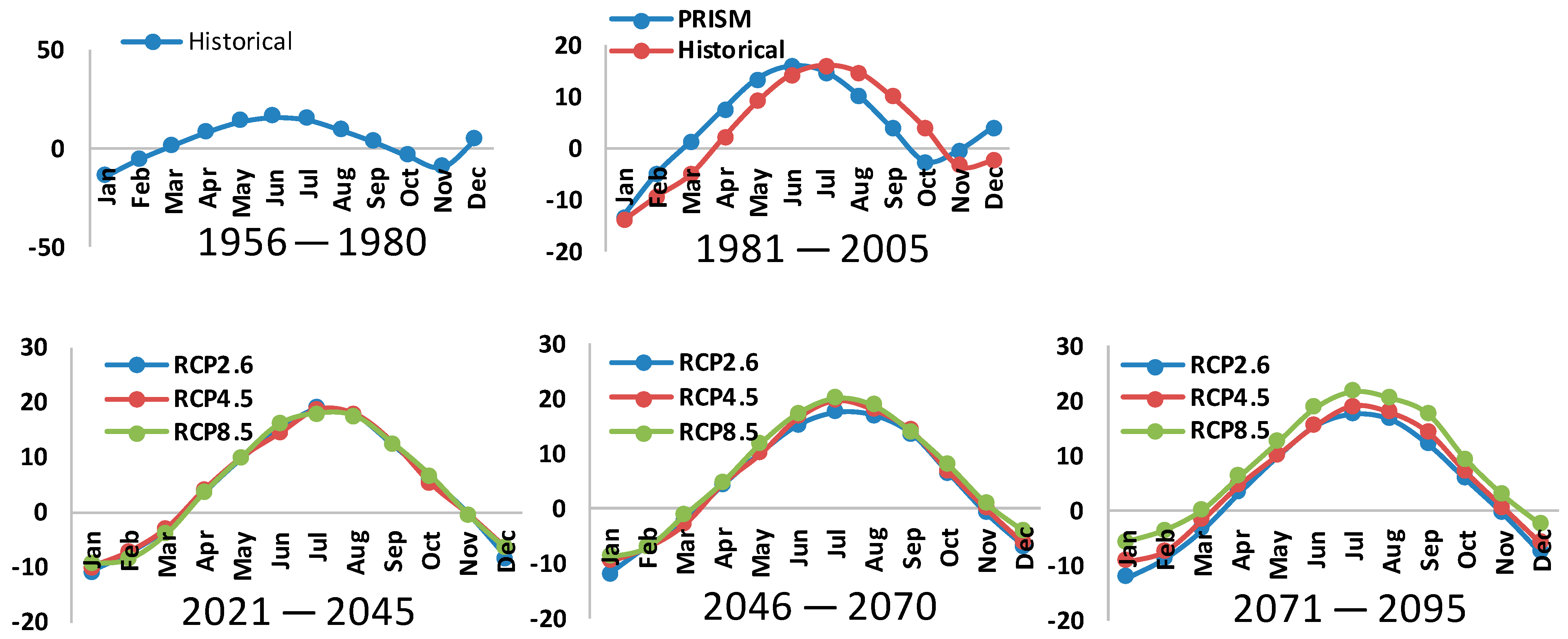
Average monthly minimum temperature patterns: Average monthly minimum temperatures were computed as the minimum temperatures for each month, averaged over the 25-year time period of the climate scenario, and then averaged across all simulated grid points. These are shown in Figure 1. These charts highlight an increasingly warmer trend as we move from early- through mid- to latter-century time periods. RCP8.5 is projected to yield the highest minimum temperatures, as expected, with noticeable increases particularly for the 2071–2095 period as compared to the other two CMIP5 projections.

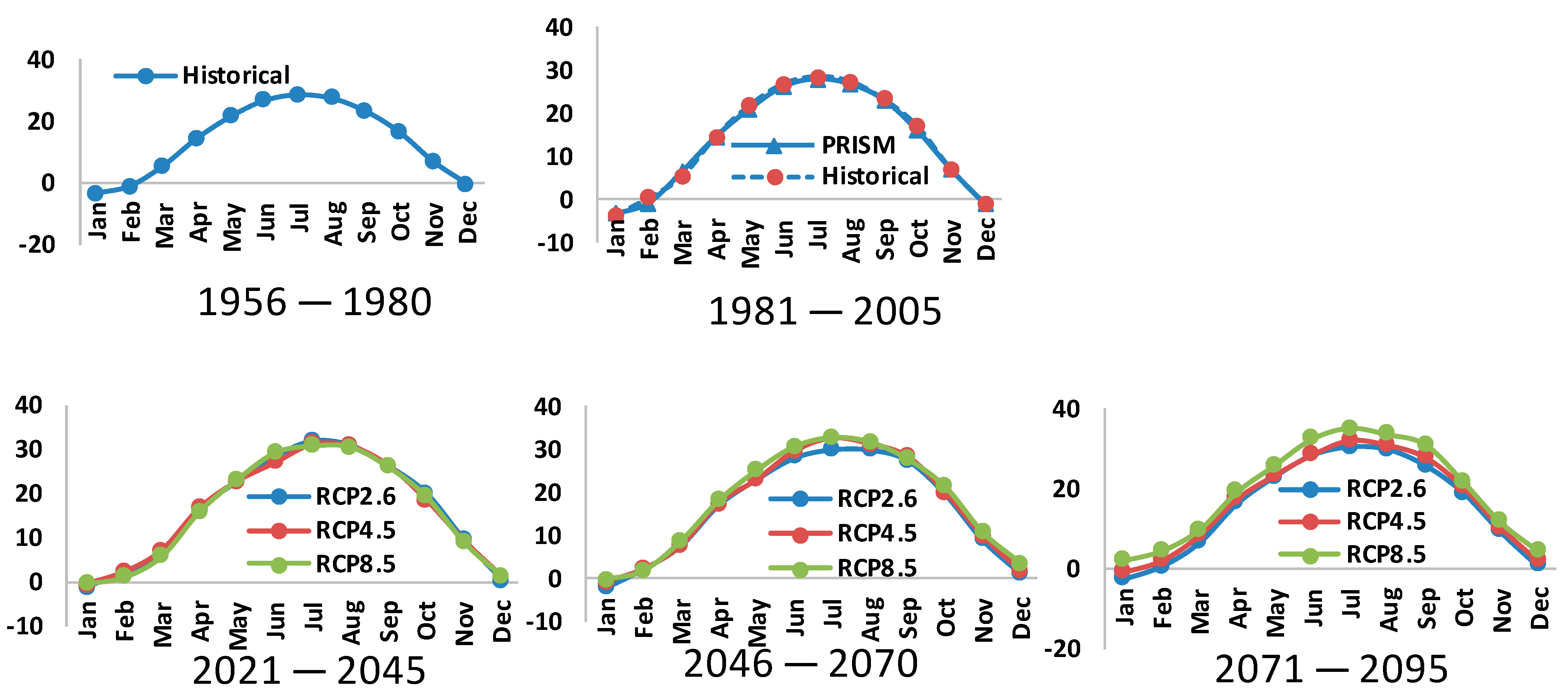
Average monthly maximum temperature patterns: Average monthly maximum temperatures were computed in a similar manner (Figure 2). They represent the maximum monthly temperatures averaged over the 25-year time horizon for reach climate scenario, and then an area-weighted average taken across all simulated grid points. RCP8.5 projections once again yield the highest monthly values. Monthly maximum temperatures are highest with the RCP8.5 projection, particularly for June through September, and January and February, which are markedly higher than the other two RCP projections.

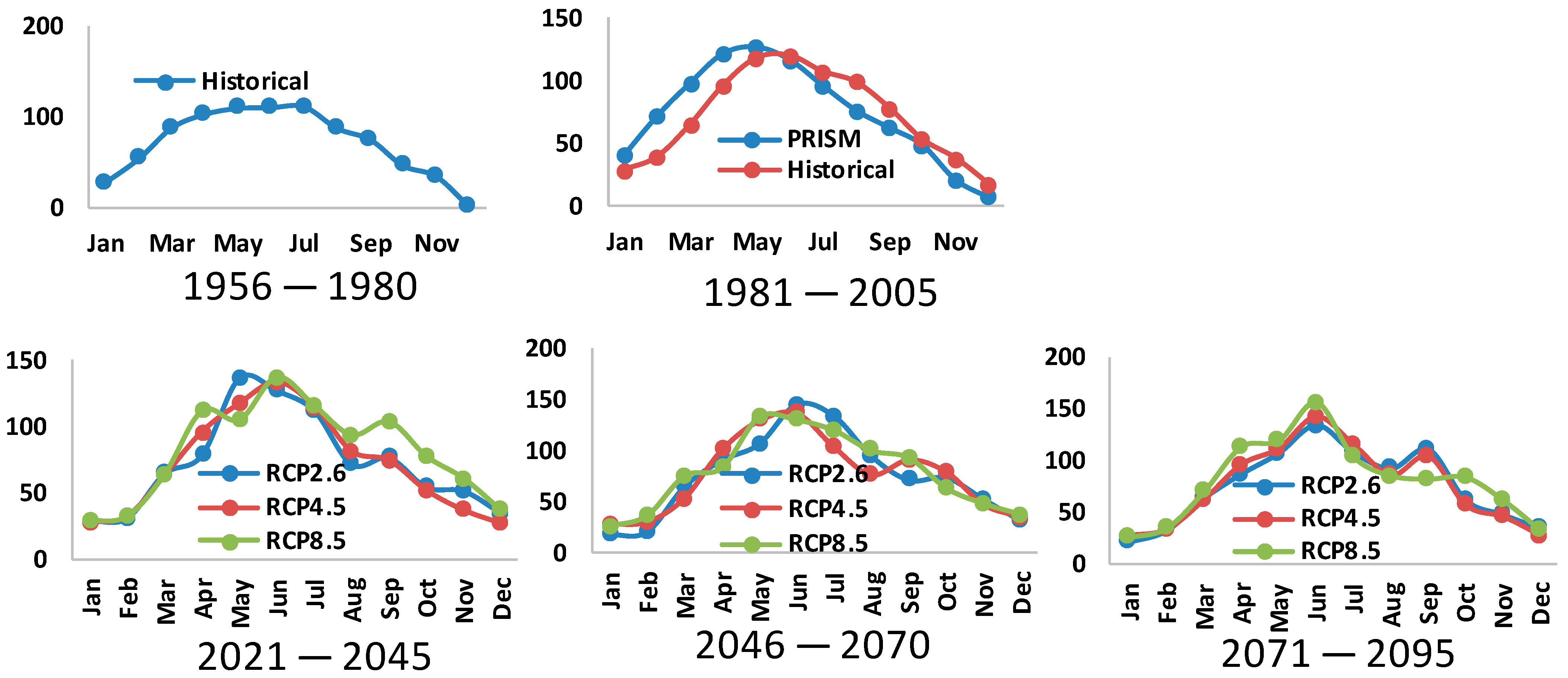
Average monthly precipitation patterns: Annual precipitation levels indicate higher overall levels for RCP8.5 as compared to current patterns and other climate projections. However, of more relevance to corn yields are precipitation levels in the growing season. Average monthly precipitation patterns are shown in Figure 3, and were computed as monthly total precipitation levels, averaged over the 25-year time period for each climate scenario, and then an area-weighted average taken across all applicable grid points associated with the crop–soil polygons. The charts indicate that the bulk of the annual precipitation increase associated with RCP8.5 for the 2021–2045 period is projected to occur in the August through November months.

2.5. APEX Corn Yield Validation for 1998–2000 Period

APEX was calibrated and validated for crop yield and edge-of-field environmental indicators (surface runoff and sediment and nutrient losses) during the UMRW study [52]. Based on interviews with producers, average continuous corn yield for the several preceding years (1997–1999) was 8.34 MT/ha on a 100% dry matter basis (equivalent to 155 bu/acre), while the average 100% dry matter yield for corn following soybeans was 8.6 MT/ha (equivalent to 160 bu/acre total weight) [57]. The reported 100% dry matter yield for soybeans was 3.22 MT/ha (equivalent to 55 bu/acre) (Osei et al., 2000). These measured values are compared to simulated values from the validated APEX model in

Table 5. APEX model validation results for 1998–2000 application in northeast Iowa.

	Measured Data		Simulated
Agronomic or Environmental Indicator	Value	Source and Notes	Value
Crop yields (MT/ha: 1997–1999 production years
Continuous corn yield (MT/ha)	8.34	Average from UMRW study [51]. Obtained from survey of producers.	8.30
Corn following soybean yield (MT/ha)	8.60		8.31
Soybean yield (MT/ha)	3.22		3.54
Surface runoff (mm)
From USEPA [59]: data by HUC *	88.3	Buchanan County: 2002	79.3
From Osei et al. [51]	65.1	Flow for UMRW	79.3
Sediment loss from fields (MT/ha)
From USEPA [59]: data by HUC *	1.66	Buchanan County: 2002	2.71
From Osei et al. [51]	2.24	Sediment loss from UMRW	2.71

* Measured data are averages for all hydrologic unit codes (HUCs) in Buchanan County, Iowa and reflect 2002 conditions.

using the PRISM gridded weather data, averaged for the same 1997–1999 time period. Additional data points are not available for computing a Nash Sutcliffe efficiency value [58] for the current set of corn yield simulations. However, the numbers in Table 5 indicate clearly that the model performs very well for corn and soybean yield estimation. Furthermore, since we are utilizing the same model setup and APEX was adequately calibrated for the UMRW study, we consider it sufficiently validated for the current study. Similar validations were accomplished for edge-of-field surface runoff and sediment losses (Table 5). All measured and simulated values compared in Table 5 are from the same time periods and comparable geographies.

APEX calibration and validation entailed minor adjustments in key APEX model parameters. For the benefit of the reader,

Table 6. Key APEX model parameters resulting from calibration/validation process.

Parameter	Description	Range	Value
PARM1	Crop canopy-PET	1–2	2
PARM3	Water stress–harvest index	0–1	0.5
PARM4	Water storage N leaching	0–1	1
PARM7	N fixation	0–1	0.9
PARM8	Soluble phosphorus runoff coefficient	10–20	20
PARM17	Soil evaporation–plant cover factor	0–0.5	0.35
PARM18	Sediment routing exponent	1–1.5	1.5
PARM19	Sediment routing coefficient	0.01–0.05	0.03
PARM45	Sediment routing travel time coefficient	0.5–10	3

displays the values of key parameters of the calibrated and validated model that were used for all simulations in this study.

2.6. Simulation Procedure

To determine the impacts of climate projections on corn and soybean yields, fields identified as corn- or soybean-growing fields were simulated using all twelve climate scenarios—including the baseline and the eleven alternative climate scenarios. Across all polygons simulated, the only difference between the scenarios was the climate regime. Thus, the model simulations for the baseline climate scenario were identical to that of the other climate scenarios except for the climate input data—daily records of precipitation, minimum temperature, and maximum temperature.

Due to the substantial number of fields (polygons)—88,322 crop-soil polygons were identified as corn-growing fields in Buchanan County, Iowa and 69,651 were identified as soybean-growing fields—a complete randomization procedure was utilized in determining the minimum number of polygons that needed to be simulated to obtain the same results as if all polygons were simulated. Once the polygons were randomized, the simulations were performed for increasing percentages of all polygons for the PRISM baseline scenario and the results stored in a database. Summary input and output data from the simulations (

Table 7. Selected input and output indicators by percentage of polygons simulated.

	Percentage of Polygons Simulated
	1%	2%	5%	10%	20%	50%	100%
Input
Average min April temperature (°C)	2.07	2.07	2.07	2.06	2.06	2.06	2.06
Average max August temperature(°C)	27.06	27.06	27.05	27.05	27.05	27.05	27.05
Annual precipitation (mm)	885.34	885.44	885.37	885.44	885.40	885.38	885.40
Average July precipitation (mm)	119.31	119.30	119.36	119.39	119.38	119.37	119.36
Average slope (%)	2.64	2.66	2.59	2.58	2.57	2.58	2.59
Moist bulk density (first layer)	1.50	1.50	1.51	1.51	1.51	1.51	1.51
Sand content (first layer) (%)	40.89	41.00	41.23	40.99	40.81	41.17	41.01
Silt content (first layer) (%)	38.06	38.01	37.82	38.03	38.18	37.90	38.02
Output (for PRISM Baseline Runs): 1981–2005 baseline
Continuous corn yields (MT/ha)	9.74	9.74	9.74	9.77	9.79	9.77	9.78
Corn after soybean yields (MT/ha)	9.80	9.80	9.81	9.83	9.84	9.83	9.84
Soybean yields (MT/ha)	3.71	3.71	3.71	3.72	3.72	3.72	3.72
Surface runoff (mm)	136.16	136.33	136.55	136.40	136.25	136.24	136.24
Sediment loss (MT/ha)	3.23	3.24	3.15	3.13	3.10	3.09	3.11

) reveal a striking similarity regardless of the percentage simulated, particularly once at least 20% of polygons had been simulated. In other words, the results obtained by simulating 20% of the randomly ordered polygons were not statistically different from the results obtained from simulating 50%, 100%, or any percentage greater than 20% of the total population of polygons. In particular, the summary data indicate that the input and output parameter averages were practically indistinguishable once at least 20% of polygons had been simulated in random order. The implication of this is that for future studies involving the same polygons, we only need to simulate 20% in order to adequately represent the economic and biophysical attributes of continuous corn and corn–soybean rotations in Buchanan County, Iowa.

3. Results and Discussion

The results presented here are area-weighted averages of crop yields on all simulated polygons. Recall that the results are based on simulation of 20% of the population of crop–soil polygons—enough to accurately represent the entire population due to random selection of the polygons, as discussed in the foregoing section. The first set of results presented (

Table 8. Simulated impacts of climate scenarios on average annual corn and soybean yields based on 1998–2000 management practices and crop genetic potential.

Scenario	1956–1980	1981–2005	2021–2045	2046–2070	2071–2095
Average annual continuous corn yields in MT/ha (% change from PRISM baseline *)
Historical (CMIP5)	7.89 (−2.3)	7.94 (−1.7)
Historical (PRISM)		8.07 (0.0)
RCP2.6 (CMIP5)			6.69 (−17.1)	7.51 (−7.0)	7.20 (−10.8)
RCP4.5 (CMIP5)			6.99 (−13.4)	6.55 (−18.9)	6.81 (−15.7)
RCP8.5 (CMIP5)			7.27 (−9.9)	6.72 (−16.8)	6.06 (−25.0)
Average annual corn following soybean yields in MT/ha (% change from PRISM baseline *)
Historical (CMIP5)	7.87 (−3.0)	7.96 (−1.9)
Historical (PRISM)		8.12 (0.0)
RCP2.6 (CMIP5)			6.72 (−17.3)	7.54 (−7.1)	7.19 (−11.5)
RCP4.5 (CMIP5)			7.01 (−13.7)	6.60 (−18.8)	6.84 (−15.8)
RCP8.5 (CMIP5)			7.28 (−10.3)	6.76 (−16.7)	6.11 (−24.8)
Average annual soybean yields in MT/ha (% change from PRISM baseline *)
Historical (CMIP5)	3.03 (−1.3)	3.19 (3.8)
Historical (PRISM)		3.07 (0.0)
RCP2.6 (CMIP5)			2.88 (−6.4)	3.43 (11.8)	3.18 (3.6)
RCP4.5 (CMIP5)			3.11 (1.4)	2.83 (−7.9)	3.12 (1.5)
RCP8.5 (CMIP5)			3.22 (4.9)	3.02 (−1.6)	2.52 (−17.8)

* Numbers in parentheses are percentage changes from 1981–2000 PRISM baseline values.

) represents the impacts of each climate scenario on corn and soybean yields, using management practices and crop genetic potential applicable to the 1998–2000 period, the period applicable to model validations. We subsequently present results from simulations based upon current (2018–2020) management practices and crop yield (genetic) potential.

3.1. Yield Impacts under 1998–2000 Management and Crop Genetic (Yield) Potential

The results in Table 8 and subsequent tables are arranged in separate sections for continuous corn, corn following soybean, and soybean in that order. In each set of results, climate scenarios are presented in rows and applicable time periods in columns. The results show crop yields in MT/ha as well as percentage changes from the PRISM baseline in parentheses. Yields for the 1981–2005 period representing the PRISM baseline are also shown. Each time period has a 25-year duration. Future climate projections are broken into three periods that cover most of the remainder of the 21st century. Hindcasted CMIP5 and actual (PRISM) scenarios cover a combined period dating back to 1956. No results are presented for 2006–2020 in Table 8 as there were no climate projections utilized for this period. A separate set of PRISM results covering the 1996–2020 period is presented in subsequent tables.

The yields shown in Table 8 and other tables are on a 100% dry weight basis. To convert to total (or wet) weight basis one would divide by 0.855 to reflect a 14.5% moisture content of corn dried for market and similarly by 0.87 to reflect a 13% moisture content of soybeans. The 1981–2005 PRISM baseline yields are indicated in the table as 8.07 MT/ha (equivalent to 150 bu/acre), 8.12 MT/ha (equivalent to 151 bu/acre), and 3.07 MT/ha (equivalent to 52 bu/acre) for continuous corn, corn following soybeans, and soybeans, respectively.

Across climate scenarios, a very consistent set of results are indicated in Table 8 for corn. For both continuous corn and corn following soybeans, future climate projections are expected to reduce corn yields substantially. The range is from 7 to 25% reduction depending on the climate scenario and time period. RCP8.5—the climate scenario with the greatest prospect for increased global mean temperatures—is associated with the highest reduction in corn yields—projected to occur in the 2071–2095 period.

Impacts of the climate scenarios on soybean yields are also noticeable, though not as substantial. The same time period associated with the greatest reduction in corn yields—2071–2095 under RCP8.5—is projected to result in the most substantial reduction in soybean yields, roughly 18%. However, soybean yields are indicated as actually improving under RCP2.6 (especially the midcentury period, 2046–2070). In fact, each RCP is associated with at least one period of improved soybean yields as compared to current climate conditions. Our results are consistent with the findings of [60], who find a 20 to 40% reduction in corn yields under projected climate change. Furthermore, the relative impacts on corn and soybean yields that we report here are consistent with the results reported by Schlenker and Roberts [2]. While the magnitudes are vastly different, they also found soybean yield reductions to be much smaller in magnitude than the projected impacts on corn yields.

It is important to note what the results in Table 8 imply. They do not indicate that corn and soybean yields will decline necessarily. They only indicate that they will be lower than what they would have been under the status quo climate regime. In particular, as we discuss later on, long-term trends in corn and soybean yields under current climate regimes have shown a substantial upward pattern. The results presented in Table 8 only indicate for instance that by the 2071–2095 period, if the RCP8.5 scenario materializes, corn yields could be 25% lower than what they would have been in that time period along the long-term yield trajectory in that county. Similar interpretations apply to the other yield impacts shown in the Table. The results in the table are essentially yield impacts conditioned upon the assumed management and crop genetic potential.

3.2. Yield Impacts under Current Management and Crop Yield Potential

Crop yield simulations under the twelve climate scenarios were replicated to reflect current management and crop yield potential in order to cast the results in a more recent context. The results (

Table 9. Simulated impacts of climate scenarios on average annual corn and soybean yields based on 2019–2021 management practices and crop genetic potential: MT/ha (% changes from PRISM).

Scenario	1956–1980	1981–2005	1996–2020	2021–2045	2046–2070	2071–2095
Average annual continuous corn yields in MT/ha (% change from PRISM baseline *)
Historical (CMIP5)	10.13 (−4.9)	10.33 (−3.0)
Historical (PRISM)		10.39 (−2.5)	10.65 (0.0)
RCP2.6 (CMIP5)				8.30 (−22.1)	9.80 (−8.0)	9.13 (−14.3)
RCP4.5 (CMIP5)				9.09 (−14.6)	8.23 (−22.7)	8.97 (−15.8)
RCP8.5 (CMIP5)				9.18 (−13.9)	8.76 (−17.8)	7.78 (−26.9)
Average annual corn following soybean yields in MT/ha (% change from PRISM baseline *)
Historical (CMIP5)	10.11 (−5.7)	10.39 (−3.1)
Historical (PRISM)		10.47 (−2.3)	10.72 (0.0)
RCP2.6 (CMIP5)				8.19 (−23.6)	9.77 (−8.9)	9.05 (−15.6)
RCP4.5 (CMIP5)				8.98 (−16.2)	8.19 (−23.6)	8.93 (−16.6)
RCP8.5 (CMIP5)				9.15 (−14.6)	8.65 (−19.3)	7.60 (−29.1)
Average annual soybean yields in MT/ha (% change from PRISM baseline *)
Historical (CMIP5)	3.28 (−3.9)	3.42 (0.3)
Historical (PRISM)		3.39 (−0.8)	3.41 (0.0)
RCP2.6 (CMIP5)				2.96 (−13.4)	3.48 (1.8)	3.24 (−5.0)
RCP4.5 (CMIP5)				3.21 (−5.9)	2.90 (−15.0)	3.18 (−6.9)
RCP8.5 (CMIP5)				3.28 (−4.0)	3.04 (−10.8)	2.58 (−24.4)

* Numbers in parentheses are percentage changes from 1996–2020 PRISM baseline values.

) reveal largely similar impacts, indicating that the percentage changes from baseline climate conditions are fairly robust. Table 9 includes an additional column representing the 1996–2020 time period. The PRISM data for this new time period is the new baseline to which all other climate scenario results will be compared. Consequently, all the percentage changes indicated in the table were computed relative to the PRISM 1996–2020 baseline.

Once again, it is important to note that the results reflect crop management and genetic potential applicable to the 2018–2020 period. Thus, the results were validated in comparison to that period, and not the entire 25-year (1996–2020) period of simulation. Simulation results reported in Table 9 for the 1996–2020 PRISM baseline compare very favorably to average crop yields for Buchanan County [1] for the 1998–2020 period. The continuous corn yield for the 1996–2020 PRISM period averaged 10.65 MT/ha (comparable to a 11.01 MT/ha reported yield average for the 1998–2020 period), equivalent to 198 bu/acre at 14.5% moisture content. Corresponding average yields for corn following soybeans (10.72 MT/ha) and soybeans (3.41 MT/ha; comparable to an average reported yield of 3.03 MT/ha for the 1998–2020 period) are also shown in the table.

As expected, corn and soybean yields for the 1996–2020 period are all greater in magnitude than indicated in the previous table for the 1981–2005 period. Furthermore, while the percentage changes for the climate scenarios are consistent with those shown in Table 8 for the previous set of simulations, they are of greater magnitude, and only one scenario is associated with a small (1.8%) increase in yields. All other scenarios show much greater reductions in yields than when 1998–2000 management and crop genetic potential were utilized. The results indicate that, compared to current yields, corn yields could be 27 to 29% lower than the long-term yield trajectory towards the end of the 21st century if RCP8.5 materializes. The other climate scenarios and time periods are not as bleak, but indicate sizable reductions in corn yields as compared to long-term trends. Similarly, soybean yields are projected to be impacted worst with the RCP8.5 scenario and towards the end of the century. It is important to note that RCP8.5 has been identified as the climate scenario most likely to materialize based upon a comparison of actual CO₂ emissions to projected emissions from all climate scenarios between 2006 and 2020 [61]

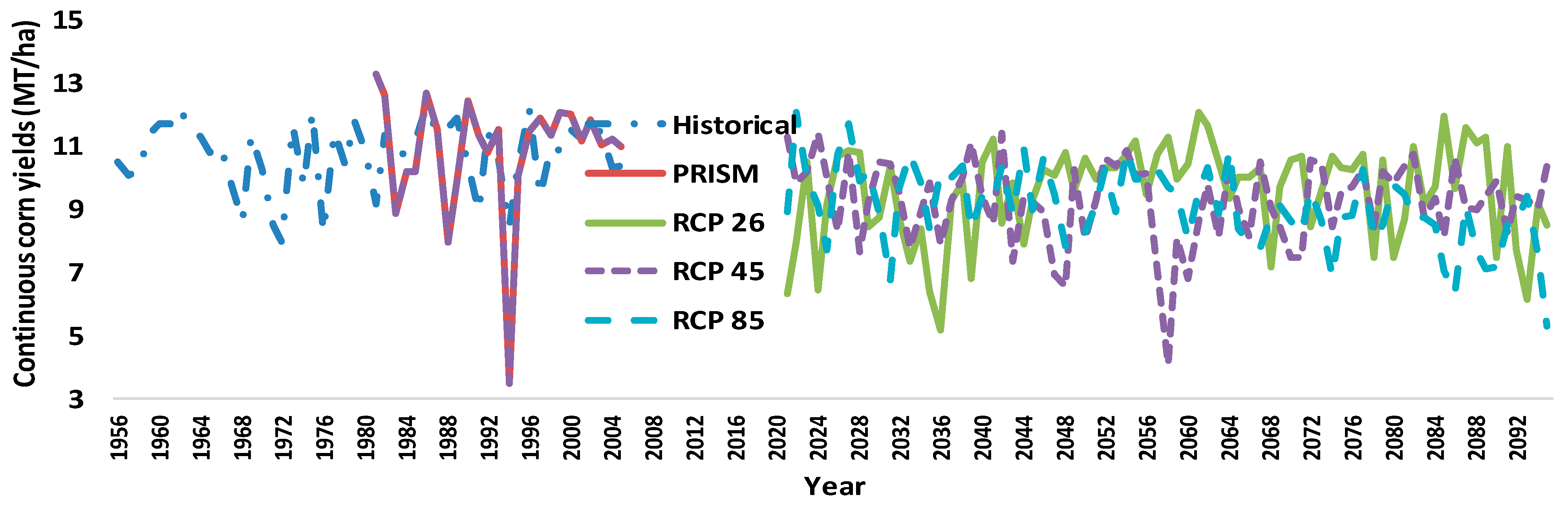
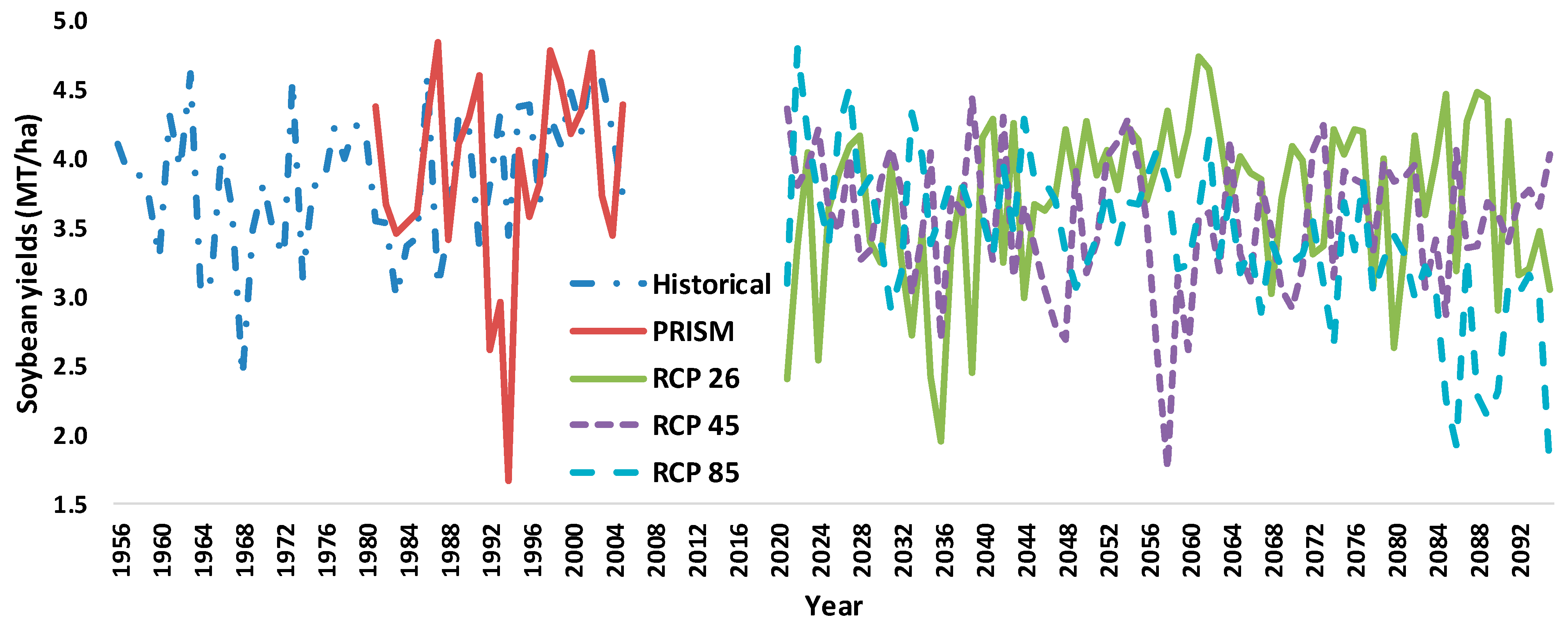
To further elucidate the impacts of climate scenarios on corn and soybean yields, we present annual trends in corn and soybean yields that are indicated by these scenarios in Figure 4, Figure 5 and Figure 6. The dynamic patterns in these charts only reflect responses to climatic factors since other biophysical parameters are held constant across all scenarios. It is clear from these charts that future climate projections will induce a yield-reducing impact as compared to the PRISM baseline or historical CMIP5 levels. However, for a given climate scenario, there are no discernible trends in corn or soybean yields. The climate impacts thus represent downward shifts in corn and soybean yields from baseline levels.

3.3. Yield Projections after Accounting for Long-Term Yield Trends

The yield impacts presented thus far for the climate scenarios have been predicated upon fixed management and crop genetic potential, first for the 1998–2000 period for validation purposes, and subsequently for the 2018–2020 period for current context. This was necessary in order to determine the impacts of climate on yields, decoupled from management and crop genetics. Having established these climate impacts, we are now in a position to obtain some actual yield projections—absolute, in contrast to relative, impacts—based on the long-term trends in corn and soybean yields. Most studies do not appear to attempt such absolute impacts, but we feel it necessary in order to set the results in the appropriate context.

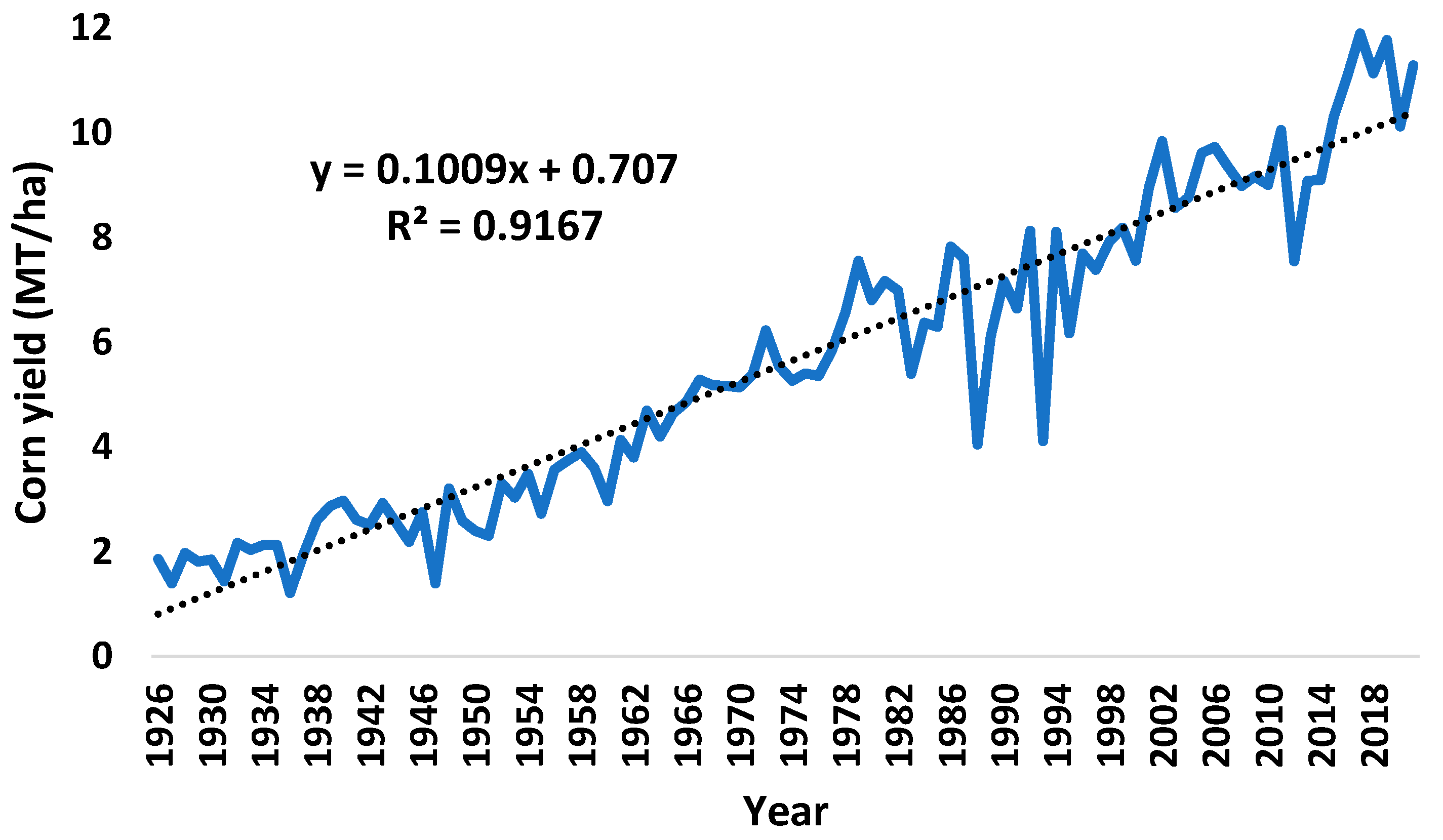
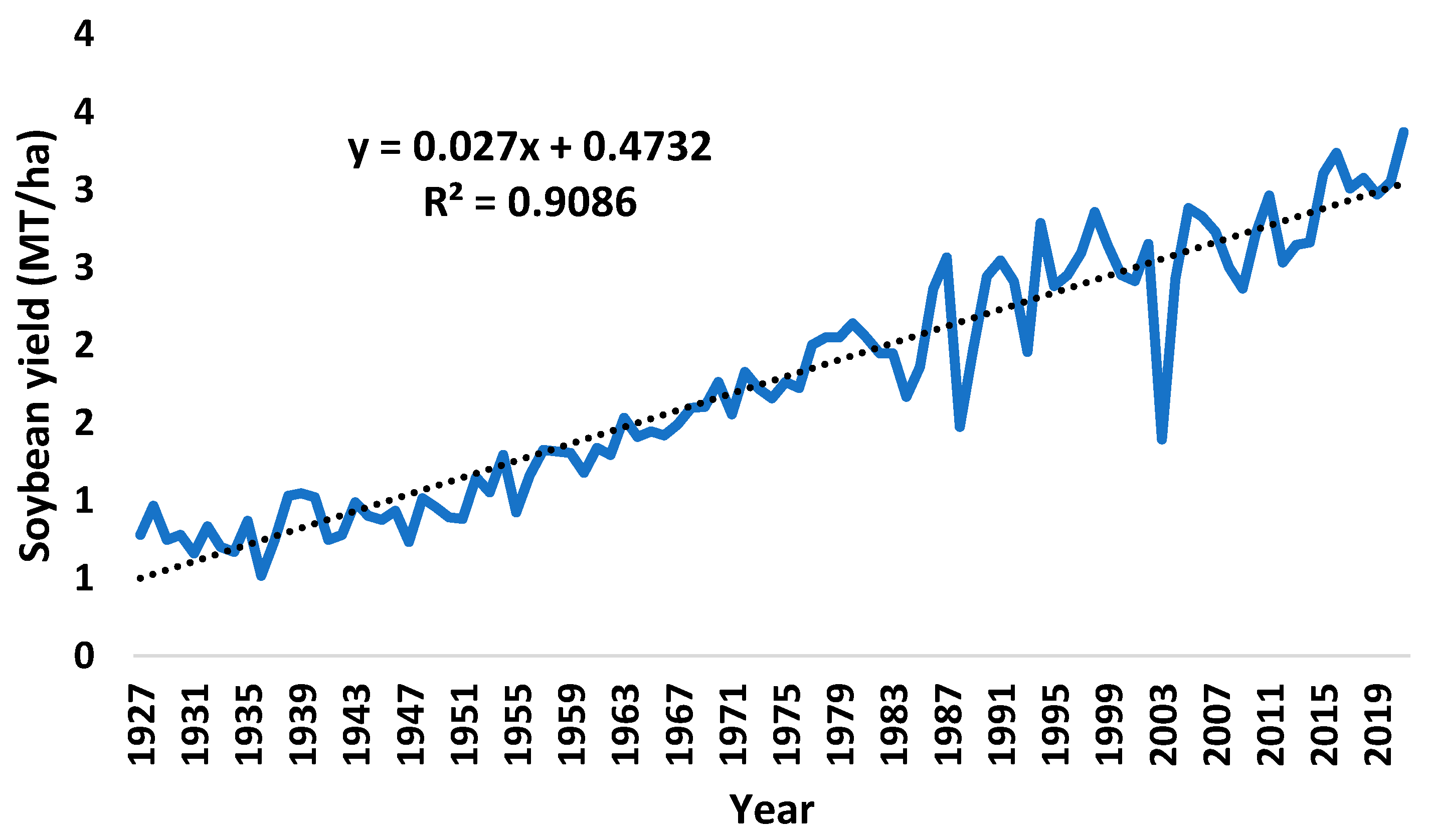
Long-term trends in corn (Figure 7) and soybean (Figure 8) yields indicate significant and sustained upward trends in crop yields over the past 90 years. Since for a given climate scenario, there were no discernible trends in crop yields as reflected in Figure 4, Figure 5 and Figure 6, it stands to reason that the long-term trends displayed in Figure 7 and Figure 8 are predominantly due to changes in crop genetics and management. To determine anticipated yields under each climate scenario, we extrapolate the yield trends through the end of the century and apply the robust climate impacts reported in Table 9. The results of this exercise are displayed in

Table 10. Simulated corn and soybean yields by climate scenario based on 2019–2021 management and crop genetics and long-term yield trends *.

Scenario	1956–1980	1981–2005	1996–2020	2021–2045	2046–2070	2071–2095
Corn yield projections based on long-term trend (MT/ha) (% change from 1996–2020 baseline)
Yield projections +	5.05 (−44.4)	7.57 (−16.7)	9.08 (0.0)	11.60 (27.8)	14.13 (55.6)	16.65 (83.3)
Average annual continuous corn yields: MT/ha (% change from PRISM baseline) by climate scenario
Historical (CMIP5)	4.80 (−47.2)	7.34 (−19.2)
Historical (PRISM)		7.38 (−18.7)	9.08 (0.0)
RCP2.6 (CMIP5)				9.04 (−0.5)	12.99 (43.0)	14.27 (57.2)
RCP4.5 (CMIP5)				9.91 (9.1)	10.92 (20.2)	14.02 (54.4)
RCP8.5 (CMIP5)				10.00 (10.1)	11.62 (27.9)	12.17 (34.0)
Average annual corn after soybean yields: MT/ha (% change from PRISM baseline) by climate scenario
Historical (CMIP5)	4.76 (−47.6)	7.34 (−19.2)
Historical (PRISM)		7.40 (−18.6)	9.08 (0.0)
RCP2.6 (CMIP5)				8.87 (−2.3)	12.87 (41.8)	14.06 (54.8)
RCP4.5 (CMIP5)				9.73 (7.1)	10.79 (18.9)	13.88 (52.8)
RCP8.5 (CMIP5)				9.90 (9.1)	11.40 (25.5)	11.80 (30.0)
Soybean yield projections based on long-term trend (MT/ha) (% change from 1996–2020 baseline)
Yield projections +	1.61 (−40.2)	2.28 (−15.1)	2.69 (0.0)	3.36 (25.1)	4.04 (50.2)	4.71 (75.4)
Average annual soybean yields: MT/ha (% change from PRISM baseline) by climate scenario
Historical (CMIP5)	1.54 (−42.5)	2.29 (−14.8)
Historical (PRISM)		2.26 (−15.8)	2.69 (0.0)
RCP2.6 (CMIP5)				2.91 (8.3)	4.11 (53.0)	4.47 (66.5)
RCP4.5 (CMIP5)				3.16 (17.7)	3.43 (27.7)	4.39 (63.3)
RCP8.5 (CMIP5)				3.23 (20.2)	3.60 (34.0)	3.56 (32.5)

* Yields in MT/ha. Numbers in parentheses are percentage changes from 1996–2020 PRISM baseline yield values. ⁺ Yield projections based on long-term yield trends and current climate patterns.

. Our reference point of comparison is still the 1996–2020 PRISM scenario, which, again, refers to current conditions and we utilize this scenario as the new baseline. Note that this exercise assumes that the long-term yield trajectory will hold through the end of the 21st century.

To obtain the numbers in Table 10, we start with the actual average yields along the long-term yield trajectory. The actual average corn yields for the entire PRISM baseline period (1996–2020) is 9.08 MT/ha, contrasted to the 2018–2020 average of 11.01 MT/ha. Projecting the yield trends using the linear regression equation for the corn trend line—$CornYield=0.707+0.1009t$ (Figure 7)—we obtain average yield projections of 11.6 MT/ha, 14.1 MT/ha, and 16.6 MT/ha (Table 10) for the 2021–2045, 2046–2070, and 2071–2095 time periods, respectively. For soybeans, the corresponding yield projections based on the current yield trajectory are 3.4 MT/ha, 4.0 MT/ha, and 4.7 MT/ha, respectively (Table 10). The soybean projections are based on the linear trend line—$SoybeanYield=0.4732+0.027t$ (Figure 8), where $t$ is time in years from the base year of 1926 for corn and 1927 for soybeans. These are the anticipated yield realizations based on the current climate regime. However, as we saw in Table 7 and Table 8, projected climate change scenarios would impact these yields significantly. Applying the percentage yield impacts presented in Table 9 to the long-term yield trajectory, we arrive at the corn and soybean yield forecasts shown in Table 10.

The yield projections shown in Table 10 indicate that with the exception of RCP2.6 in the immediate future (2021–2046 period), corn and soybean yields are expected to increase significantly from current (1996–2020) levels. In general, corn yields are expected to increase by roughly 7 to 10% during the 2021–2045 period under RCP4.5 and RCP8.5. In the subsequent period (2046–2070), they are supposed to trend up to 20 to 40% above current levels, and by the end of the century, they would increase further to 30 to 60% above current levels depending upon the climate scenario that materializes. By the end of the century, RCP8.5 is projected to be the climate scenario least conducive to growth in corn yields. In the absence of projected climate change, the corn yields would likely have followed the long-term trajectory to achieve levels that are substantially higher: about 28% higher in the 2021–2045 period, 55% higher in the subsequent period, and over 80% higher by the end of the century.

Soybean yields are projected to increase regardless of climate scenario once we factor in the long-term yield trajectory (Table 10). As with the foregoing discussion about corn, soybean yields will trend upward, with the highest yields toward the end of the century (2071–2095 period). Under RCP2.6, soybean yields are projected to be roughly 66% higher than current levels by the end of the century. In contrast, they are projected to be only 32% higher than current levels in the same time period under RCP8.5. In comparison, if current climate patterns remain in place—that is, projected warming trends are averted—and the long-term soybean yield trajectory is maintained, the yields would be over 75% higher than current levels by the end of the century.

The results presented in Table 10 indicate that while the climate change scenarios are projected to depress corn and soybean yields as compared to the long-term trends, the impacts are not large enough to result in an outright yield decline in most instances. Under most climate change scenarios and for most time periods, we can expect corn and soybean yields in Buchanan County, Iowa to trend upwards from current levels. However, the impacts of the climate change scenarios indicate that the upward trends would be measured. Instead of an 83% increase in corn yields, we may see a 30 to 50% increase and instead of a 75% increase in soybean yields, we may see a 30 to 60% increase.

4. Conclusions

Projected changes in climate largely indicate a warming trend with impacts on crop production that have not been adequately addressed. This paper contributes to our understanding of the impacts of anticipated changes in climate trends by estimating the impacts on corn and soybean yields in a county in the middle of the Corn Belt, where previous efforts have established data and validated models. Utilizing the most widely used climate scenarios, we estimated the impacts of projected climate patterns on the yields of continuous corn, corn following soybeans, and soybeans through the remainder of the 21st century.

The results of this study indicate that by the end of the century, corn yields could be up to 29% lower than long-term yield trends would indicate depending on the specific climate scenario that materializes. Of the three main climate scenarios—RCP2.6, RCP4.5, and RCP8.5—RCP8.5 is associated with the greatest impact on corn yields, with a 29% reduction in corn following soybean yields towards the end of the century. Similar results are obtained for soybeans, where yields could be up to 24% lower under RCP8.5 towards the end of the century, as compared to current climate patterns.

While the results call for yield reductions due to the projected climate change scenarios relative to long-term yield trends, these do not indicate that yields would absolutely decline. While corn and soybean yields would in fact be lower under these climate scenarios than the status quo climate regime, the yields would nonetheless increase in an absolute sense, due to the fact that the projected climate-change-induced yield reductions are not sufficient in magnitude to completely offset the elevation in yields along the long-term yield trajectory that is driven largely by changes in crop management and crop genetic potential.

It is important to note that the projected increases in corn and soybean yields are predicated on the robustness of the long-term yield trajectory. However, the actual yield trajectory is highly sensitive to future agronomic uncertainties driven by producer utilization of agrochemicals, nutrients, and prevailing environmental concerns, and how these are affected by consumer perceptions. Given contemporary patterns and trends in consumer and environmental advocacy and the influence they wield upon commodity supply chains, it is extremely difficult to predict producer input use decades in advance, much less their consequent impacts on crop yields. Nonetheless, it is likely that corn and soybean yields will continue to rise, though hampered somewhat by the impacts of climate change projections.

References

- USDA NASS (National Agricultural Statistics Service). Census of Agriculture; U.S. Department of Agri-Culture, National Agricultural Statistics Service: Washington, DC, USA, 2022. Available online: https://www.nass.usda.gov/AgCensus/index.phphttps://www.nass.usda.gov/AgCensus/index.php (accessed on 29 October 2022).
- Schlenker, W.; Roberts, M.J. Non-linear temperatures effect indicate severe damage to US crops un-der climate change. Proc. Natl. Acad. Sci. USA 2009, 106, 37. [Google Scholar] [CrossRef] [PubMed] [Green Version]
- Jin, Z.; Zhuang, Q.; Wang, J.; Archontoulis, S.V.; Zobel, Z.; Kotamarthi, V.R. The combined and separate impacts of climate extremes on the current and future US rainfed maize and soybean production under elevated CO2. Glob. Chang. Biol. 2017, 23, 2687–2704. [Google Scholar] [CrossRef] [PubMed]
- Kornprobst, A.; Davison, M. Climate Change Influence on Ontario Corn Farms’ Income. Environ. Model. Assess. 2022, 27, 399–411. [Google Scholar] [CrossRef]
- Pryor, S.C.; Scavia, D.; Downer, C.; Gaden, M.; Iverson, L.; Nordstrom, R.; Patz, J.; Robertson, G.P. Ch. 18: Midwest. Climate Change Impacts in the United States: The Third National Climate Assessment; Melillo, J.M., Richmond, T., Yohe, G.W., Eds.; U.S. Global Change Research Program: Washington, DC, USA, 2014; pp. 418–440. [CrossRef]
- Gupta, S. Climate Change Is Hurting U.S. Corn Farmers—and Your Wallet. 2017. Available online: https://edition.cnn.com/ (accessed on 20 April 2017).
- Hatfield, J.L.; Prueger, J.H. Temperature extremes: Effect on plant growth and development. Weather Clim. Extrem. 2015, 10, 4–10. [Google Scholar] [CrossRef] [Green Version]
- Chemeris, A.; Liu, Y.; Ker, A.P. Insurance subsidies, climate change, and innovation: Implications for crop yield resiliency. Food Policy 2022, 108, 102232. [Google Scholar] [CrossRef]
- Sharma, R.K.; Kumar, S.; Vatta, K.; Bheemanahalli, R.; Dhillon, J.; Reddy, K.N. Impact of recent climate change on corn, rice, and wheat in southeastern USA. Sci. Rep. 2022, 12, 16928. [Google Scholar] [CrossRef]
- Machado, S.; Bynum, E.D.; Archer, T.L.; Bordovsky, J.; Rosenow, D.T.; Peterson, C.; Bronson, K.; Nesmith, A.D.M.; Lascano, R.J.; Wilson, L.T.; et al. Spatial and Temporal Variability of Sorghum Grain Yield: Influ-ence of Soil, Water, Pests, and Diseases Relationships. Precis. Agric. 2002, 3, 389–406. [Google Scholar] [CrossRef]
- Lambert, D.K. Historical Impacts of Precipitation and Temperature on Farm Production in Kansas. J. Agric. Appl. Econ. 2014, 46, 439–456. [Google Scholar] [CrossRef] [Green Version]
- Dell, M.; Jones, B.F.; Olken, B.A. What Do We Learn from the Weather? The New Climate-Economy Literature. J. Econ. Lit. 2014, 52, 740–798. [Google Scholar] [CrossRef] [Green Version]
- Parajuli, P.; Jayakody, P.; Sassenrath, G.; Ouyang, Y. Assessing the impacts of climate change and tillage practices on stream flow, crop and sediment yields from the Mississippi River Basin. Agric. Water Manag. 2016, 168, 112–124. [Google Scholar] [CrossRef] [Green Version]
- Arnold, J.G.; Moriasi, D.N.; Gassman, P.W.; Abbaspour, K.C.; White, M.J.; Srinivasan, R.; Santhi, C.; Harmel, R.D.; van Griensven, A.; Van Liew, M.W.; et al. SWAT: Model Use, Calibration, and Validation. Trans. ASABE 2012, 55, 1491–1508. [Google Scholar] [CrossRef]
- Arnold, J.G.; Srinivasan, R.; Muttiah, R.S.; Williams, J.R. LARGE AREA HYDROLOGIC MODELING AND ASSESSMENT PART I: MODEL DEVELOPMENT. JAWRA J. Am. Water Resour. Assoc. 1998, 34, 73–89. [Google Scholar] [CrossRef]
- Williams, J.R.; Arnold, J.G.; Kiniry, J.R.; Gassman, P.W.; Green, C.H. History of model development at Temple, Texas. Hydrol. Sci. J. 2008, 53, 948–960. [Google Scholar] [CrossRef] [Green Version]
- Williams, J.R.; Arnold, J.G.; Srinivasan, R. The APEX Model. BRC Report No. 00-06, Blackland Research Center, Texas Agricultural Experiment Station, Texas Agricultural Extension Service; Texas A&M University System: Temple, TX, USA, 2000. [Google Scholar]
- Steglich, E.M.; Osorio, J.; Doro, L.; Jeong, J.; Williams, J. Agricultural Policy/Environmental eXtender: User’s Manual Version 1501. AgriLIFE Research; Texas A&M System, Blackland Research and Extension Center: Temple, TX, USA, 2019; Available online: https://epicapex.tamu.edu/manuals-and-publications/ (accessed on 1 November 2022).
- Liverman, D.M. Vulnerability to drought in Mexico; the cases of Sonara and Pubela in 1970. Ann. Assoc. Am. Geogr. 1990, 80, 49–72. [Google Scholar] [CrossRef]
- Shuaizhang, F.; Krueger, A.; Oppenheimer, M. Linkages among climate change yields and Mexi-co-US cross border migration. Proc. Natl. Acad. Sci. USA 2010, 107, 14257–14262. [Google Scholar]
- Jayachandran, S. Selling Labor Low: Wage Responses to Productivity Shocks in Developing Countries. J. Politics Econ. 2006, 114, 538–575. [Google Scholar] [CrossRef] [Green Version]
- Levine, D.; Young, D. The Impact of Rainfall on Rice Output in Indonesia. NBER 2014, Working Paper No. 20302. July 2014. Available online: http://www.nber.org/papers/w20302.pdf (accessed on 1 November 2022).
- Deschena, O.; Greenstone, M. The economic impacts of climate change; evidence from Agricultural output and random fluctuations. Am. Econ. Rev. 2007, 97, 354–385. [Google Scholar] [CrossRef] [Green Version]
- Bezner Kerr, R.; Hasegawa, T.; Lasco, R.; Bhatt, I.; Deryng, D.; Farrell, A.; Gurney-Smith, H.; Ju, H.; Lluch-Cota, S.; Meza, F.; et al. Food, Fibre, and Other Ecosystem Products. In Climate Change 2022: Impacts, Adaptation and Vulnerability; Contribution of Working Group II to the Sixth Assessment Report of the Intergovernmental Panel on Climate Change; Pörtner, H.-O., Roberts, D., Tignor, M., Poloczanska, E., Mintenbeck, K., Alegría, A., Craig, M., Langsdorf, S., Löschke, S., Möller, V., et al., Eds.; Cambridge University Press: Cambridge, UK; New York, NY, USA, 2022; pp. 713–906. [Google Scholar]
- FAO. Climate Change and Food Security: Risks and Responses; Food and Agriculture Organization of the United Nations: Rome, Italy, 2016; Available online: https://www.fao.org/3/i5188e/I5188E.pdf (accessed on 18 January 2023).
- Climate Change: Unpacking the Burden on Food Safety. Food Safety and Quality Series No. 8. Rome. 2020. Available online: https://doi.org/10.4060/ca8185en (accessed on 1 November 2022).
- USDA-NASS. Iowa’s Rank in United States Agriculture; U.S. Department of Agriculture, National Agricultural Statistics Service: Washington, DC, USA, 2022. Available online: https://www.nass.usda.gov/Sta-tis-tics_by_State/Iowa/Publications/Rankings/IA-2022-Rankings.pdf (accessed on 1 November 2022).
- Gassman, P.W.; Williams, J.R.; Wang, X.; Saleh, A.; Osei, E.; Hauck, L.M.; Izaurralde, R.C.; Flowers, J.D. The Agricultural Policy/Environmental eXtender (APEX) Model: An emerging tool for landscape and watershed environmental analyses. Trans. ASABE 2010, 53, 711–740. [Google Scholar] [CrossRef] [Green Version]
- Wang, X.; Williams, J.R.; Gassman, P.W.; Baffaut, C.; Izaurralde, R.; Jeong, J.; Kiniry, J.R. EPIC and APEX: Model Use, Calibration, and Validation. Trans. ASABE 2012, 55, 1447–1462. [Google Scholar] [CrossRef]
- Saleh, A.; Niraula, R.; Marek, G.W.; Gowda, P.H.; Brauer, D.K.; Howell, T.A. Lysimetric evaluation of the APEX model to simulate daily ET for irrigated crops in the Texas High Plains. Trans. ASABE 2018, 61, 65–74. [Google Scholar] [CrossRef]
- Tadesse, H.K.; Moriasi, D.N.; Gowda, P.H.; Marek, G.; Steiner, J.L.; Brauer, D.; Talebizadeh, M.; Nelson, A.; Starks, P. Evaluating evapotranspiration estimation methods in APEX model for dryland cropping systems in a semi-arid region. Agric. Water Manag. 2018, 206, 217–228. [Google Scholar] [CrossRef]
- Timlin, D.; Chun, J.A.; Meisinger, J.; Kang, K.; Fleisher, D.; Staver, K.; Doherty, C.; Russ, A. Evaluation of the agricultural policy environmental extender (APEX) for the Chesapeake Bay watershed. Agric. Water Manag. 2019, 221, 477–485. [Google Scholar] [CrossRef]
- Worqlul, A.W.; Jeong, J.; Green, C.H.M.; Abitew, T.A. The impact of rainfall distribution methods on streamflow throughout multiple elevations in the Rocky Mountains using the APEX model—Price River watershed, Utah. J. Environ. Qual. 2021, 50, 1395–1407. [Google Scholar] [CrossRef] [PubMed]
- Cheng, G.; Harmel, R.; Ma, L.; Derner, J.; Augustine, D.; Bartling, P.; Fang, Q.; Williams, J.; Zilverberg, C.; Boone, R.; et al. Evaluation of APEX modifications to simulate forage production for grazing management decision-support in the Western US Great Plains. Agric. Syst. 2021, 191, 103139. [Google Scholar] [CrossRef]
- Carroll, S.; Le, K.; Moreno-García, B.; Runkle, B. Simulating Soybean–Rice Rotation and Irrigation Strategies in Arkansas, USA Using APEX. Sustainability 2020, 12, 6822. [Google Scholar] [CrossRef]
- Gautam, S.; Mbonimpa, E.G.; Kumar, S.; Bonta, J.V.; Lal, R. Agricultural Policy Environmental eXtender model simulation of climate change impacts on runoff from a small no-till watershed. J. Soil Water Conserv. 2015, 70, 101–109. [Google Scholar] [CrossRef]
- Mason, R.; Merrill, S.; Görres, J.; Faulkner, J.; Niles, M. Agronomic and environmental performance of dairy farms in a warmer, wetter climate. J. Soil Water Conserv. 2021, 76, 76–88. [Google Scholar] [CrossRef]
- Raj, A.D.; Kumar, S.; Sooryamol, K. Modelling climate change impact on soil loss and erosion vulnerability in a watershed of Shiwalik Himalayas. Catena 2022, 214, 106279. [Google Scholar] [CrossRef]
- Ford, W.; King, K.; Williams, M.; Fausey, N. Sensitivity Analysis of the Agricultural Policy/Environmental eXtender (APEX) for Phosphorus Loads in Tile-Drained Landscapes. J. Environ. Qual. 2015, 44, 1099–1110. [Google Scholar] [CrossRef]
- Hong, E.-M.; Park, Y.; Muirhead, R.; Jeong, J.; Pachepsky, Y.A. Development and evaluation of the bacterial fate and transport module for the Agricultural Policy/Environmental eXtender (APEX) model. Sci. Total Environ. 2018, 615, 47–58. [Google Scholar] [CrossRef]
- Kim, D.-H.; Jang, T.; Hwang, S. Evaluating impacts of climate change on hydrology and total nitrogen loads using coupled APEX-paddy and SWAT models. Paddy Water Environ. 2020, 18, 515–529. [Google Scholar] [CrossRef]
- Kamruzzaman, M.; Hwang, S.; Choi, S.-K.; Cho, J.; Song, I.; Song, J.-H.; Jeong, H.; Jang, T.; Yoo, S.-H. Evaluating the Impact of Climate Change on Paddy Water Balance Using APEX-Paddy Model. Water 2020, 12, 852. [Google Scholar] [CrossRef] [Green Version]
- Kamruzzaman, M.; Hwang, S.; Choi, S.-K.; Cho, J.; Song, I.; Jeong, H.; Song, J.-H.; Jang, T.; Yoo, S.-H. Prediction of the effects of management practices on discharge and mineral nitrogen yield from paddy fields under future climate using APEX-paddy model. Agric. Water Manag. 2020, 241, 106345. [Google Scholar] [CrossRef]
- Bailey, R.T.; Tasdighi, A.; Park, S.; Tavakoli-Kivi, S.; Abitew, T.; Jeong, J.; Green, C.H.; Worqlul, A.W. APEX-MODFLOW: A New integrated model to simulate hydrological processes in watershed systems. Environ. Model. Softw. 2021, 143, 105093. [Google Scholar] [CrossRef]
- Gassman, P.W.; Osei, E.; Saleh, A.; Rodecap, J.; Norvell, S.; Williams, J. Alternative practices for sediment and nutrient loss control on livestock farms in northeast Iowa. Agric. Ecosyst. Environ. 2006, 117, 135–144. [Google Scholar] [CrossRef]
- Williams, J.R.; Jones, C.A.; Dyke, P.T. A Modeling Approach to Determining the Relationship Between Erosion and Soil Productivity. Trans. ASAE 1984, 27, 0129–0144. [Google Scholar] [CrossRef]
- Williams, J.R. The erosion-productivity impact calculator (EPIC) model: A case history. Philos. Trans. R. Soc. B Biol. Sci. 1990, 329, 421–428. [Google Scholar] [CrossRef]
- Saleh, A.; Gallego, O.; Osei, E.; Lal, H.; Gross, C.; McKinney, S.; Cover, H. Nutrient Tracking Tool--a user-friendly tool for calculating nutrient reductions for water quality trading. J. Soil Water Conserv. 2011, 66, 400–410. [Google Scholar] [CrossRef]
- USDA-NASS. USDA National Agricultural Statistics Service Cropland Data Layer. 2022. Published Crop-Specific Data Layer. Available online: https://nassgeodata.gmu.edu/CropScape/ (accessed on 12 February 2022).
- USDA-NRCS. Soil Survey Staff, Natural Resources Conservation Service, United States Department of Agriculture. Soil Survey Geographic (SSURGO) Database. 2022. Available online: https://websoilsurvey.nrcs.usda.gov (accessed on 21 November 2022).
- Osei, E.; Gassman, P.; Saleh, A. Livestock and the Environment: A National Pilot Project: CEEOT–LP Modeling for the Upper Maquoketa River Watershed, Iowa; Technical Report. Report No. RR0001; Texas Institute for Applied Environmental Research, Tarleton State University: Stephenville, TX, USA, 2000. [Google Scholar]
- Keith, G.; Norvell, S.; Jones, R.; Maquire, C.; Osei, E.; Saleh, A.; Gassman, P.; Rodecap, J. Livestock and the Environment: A National Pilot Project: CEEOT-LP Modeling for the Upper Maquoketa River Watershed, Iowa; Final Report. Report No. PR0003; Texas Institute for Applied Environmental Research, Tarleton State University: Stephenville, TX, USA, 2000. [Google Scholar]
- PRISM Climate Group. PRISM Climate Group, Oregon State University. 2022. Available online: https://prism.oregonstate.edu (accessed on 21 November 2022).
- NCAR. National Centr for Atmospheric Research: Earth System Grid Portal, Climate Data Gateway. 2022. Available online: https://www.earthsystemgrid.org/ (accessed on 21 November 2017).
- Monaghan, A.J.; Steinhoff, D.F.; Bruyere, C.L.; Yates, D. NCAR CESM Global Bias-Corrected CMIP5 Output to Support WRF/MPAS Research. Research Data Archive at the National Center for Atmospheric Research, Computational and Information Systems Laboratory. Available online: https://doi.org/10.5065/d6dj5cn4 (accessed on 8 November 2022).
- IPCC. Climate Change 2013: The Physical Science Basis. In Contribution of Working Group I to the Fifth Assessment Report of the Intergovernmental Panel on Climate Change; Stocker, T.F., Qin, D., Plattner, G.-K., Tignor, M., Allen, S., Boschung, J., Nauels, A., Xia, Y., Bex, V., Midgley, P., Eds.; Cambridge University Press: Cambridge, UK; New York, NY, USA, 2013; p. 1535. Available online: https://www.ipcc.ch/site/assets/uploads/2018/02/WG1AR5_all_final.pdf (accessed on 28 July 2022).
- Taylor, K.E.; Stouffer, R.J.; Meehl, G.A. An Overview of CMIP5 and the Experiment Design. Bull. Am. Meteorol. Soc. 2012, 93, 485–498. [Google Scholar] [CrossRef] [Green Version]
- Krause, P.; Boyle, D.P.; Bäse, F. Comparison of different efficiency criteria for hydrological model assessment. Adv. Geosci. 2005, 5, 89–97. [Google Scholar] [CrossRef] [Green Version]
- USEPA. EnviroAtlas Data Download. National Table Downloads. 2022. Available online: https://www.epa.gov/enviroatlas/forms/enviroatlas-data-download (accessed on 11 November 2022).
- Leng, G.; Huang, M. Crop yield response to climate change varies with crop spatial distribution pattern. Sci. Rep. 2017, 7, 1463. [Google Scholar] [CrossRef] [PubMed] [Green Version]
- Schwalm, C.R.; Glendon, S.; Duffy, P.B. RCP8.5 tracks cumulative CO2 emissions. Proc. Natl. Acad. Sci. USA 2020, 117, 19656–19657. [Google Scholar] [CrossRef] [PubMed]
Figure 1.
Trends in monthly average minimum temperature (°C) patterns for each climate scenario.
Figure 2.
Trends in monthly average maximum temperature (°C) patterns for each climate scenario.
Figure 3.
Trends in monthly average precipitation patterns (mm) for each climate scenario.
Figure 4.
Graph of annual simulated continuous corn yields by climate scenario.
Figure 5.
Graph of annual simulated corn following soybean yields by climate scenario.
Figure 6.
Graph of annual simulated soybean yields by climate scenario.
Figure 7.
Long-term trend in historical corn yields for Buchanan County, Iowa.
Figure 8.
Long-term trend in historical soybean yields for Buchanan County, Iowa.